Probing the Global Dust Properties and Cluster Formation Potential of the Giant Molecular Cloud G148.2400.41 Probing the Global Dust Properties and Cluster Formation Potential of the Giant Molecular Cloud G148.2400.41–References
Abstract
Clouds more massive than about M⊙ are potential sites of massive cluster formation. Studying the properties of such clouds in the early stages of their evolution offers an opportunity to test various cluster formation processes. We make use of CO, , and UKIDSS observations to study one such cloud, G148.24+00.41. Our results show the cloud to be of high mass ( M⊙), low dust temperature ( 14.5 K), nearly circular (projected radius 26 pc), and gravitationally bound with a dense gas fraction of % and a density profile with a power-law index of . Comparing its properties with those of nearby molecular clouds, we find that G148.24+00.41 is comparable to the Orion-A molecular cloud in terms of mass, size, and dense gas fraction. From our analyses, we find that the central area of the cloud is actively forming protostars and is moderately fractal with a Q-value of 0.66. We also find evidence of global mass-segregation in the cloud, with a degree of mass-segregation (. We discuss these results along with the structure and compactness of the cloud, the spatial and temporal distribution of embedded stellar population, and their correlation with the cold dust distribution, in the context of high-mass cluster formation. Comparing our results with models of star cluster formation, we conclude that the cloud has the potential to form a cluster in the mass range 2000–3000 M⊙ through dynamical hierarchical collapse and assembly of both gas and stars.
Keywords:
stars: formation; Stars, ISM: clouds; Interstellar Medium (ISM), Nebulae, galaxies: clusters: general; Galaxies1 Introduction
Giant molecular clouds (GMCs) are the cradles of young star clusters (Chevance et al. 2022) in which most stars form (Lada & Lada 2003). Massive to intermediate-mass clusters play a dominant role in the evolution and chemical enrichment of the Galaxy via stellar feedback such as photoionization, stellar winds, and supernovae (Geen et al. 2015; Geen et al. 2016; Kim et al. 2018, e.g.). Understanding cluster formation, in particular the formation of intermediate-mass ( M⊙; Weisz et al. 2015) to high-mass clusters ( M⊙; Portegies Zwart et al. 2010), is therefore crucial and one of the key problems in modern astrophysics (Longmore et al. 2014; Krause et al. 2020; Krumholz & McKee 2020, e.g.). Young massive clusters (Portegies Zwart et al. 2010, YMCs;) are thought to be the potential modern-day analogues of globular clusters (GCs) that formed in the early Universe. Determining their formation mechanism will better constrain the different cluster formation models over the full mass range of clusters.
The general consensus is that GMCs convert –10% of their mass into stars before being dispersed (Evans et al. 2009; Lada, Lombardi, & Alves 2010). In this regard, massive bound clouds with mass M⊙ are the potential formation sites for massive stellar clusters of mass M⊙, assuming the star-formation efficiency is as low as 5%. Only a handful of YMCs have been found in our Galaxy (Portegies Zwart et al. 2010, e.g. see Table 2 of), despite the fact that it hosts many high-mass clouds (Solomon et al. 1987, e.g. see Figure 2 of).
Studies of Galactic disk clouds, suggest that clouds with a relatively high dense gas fraction (Lada, Lombardi, & Alves 2010, i.e. fraction of gas with 104 cm-3, or N(H2) 6.7 1021 cm-2 with respect to the total gas of the cloud;) are the sites of richer star formation (Lada et al. 2012; Evans et al. 2014), while other studies suggest that the Galactic environment plays a significant role in defining the initial conditions of star-formation in molecular clouds (Henshaw et al. 2022, e.g. Galactic centre clouds, see review by). The geometry and structure of molecular clouds also likely play a crucial role in the formation and growth of star clusters (Burkert & Hartmann 2004; Heitsch et al. 2008; Pon et al. 2012; Clarke & Whitworth 2015; Heigl, Hoemann, & Burkert 2022; Hoemann, Heigl, & Burkert 2022, e.g.).
Determining and evaluating the physical conditions, kinematics, structures, and dynamics of GMCs at their initial stages of evolution are crucial for finding the favourable conditions that a GMC requires to produce a massive cluster. In this context, massive clouds of mass M⊙, where stellar feedback effects are not yet significant, are potential targets for studying early phases of cluster formation. The molecular cloud - G148.24+00.41, the focus of the present work, is one such cloud whose properties, structure, and star-formation potential remain largely unexplored.
1.1 G148.24+00.41 Cloud
At submillimeter and millimeter wavelengths, Planck observations (Planck Collaboration et al. 2011) have revealed a population of dense molecular cold clumps and clouds in our Galaxy. The Planck Early Release Compact Source Catalog (Planck Collaboration et al. 2011, PERCSC;) provides lists of positions and flux densities of the sources in nine frequencies in the range 30–870 GHz with beam sizes ranging from 33′ to 5′. The PERCSC source “G148.24+00.41” corresponds to a cloud (ID: 2182) identified by Miville-Deschênes et al. 2017, using low-resolution (beam 8.5′) 12CO data at 115 GHz. Its temperature as estimated by Planck is around 13.5 K, while its mass as estimated by Miville-Deschênes et al. 2017 is 1.3 105 M⊙, suggesting that G148.24+00.41 is a massive cold cloud. The cloud area also includes the dark cloud “TGU 942P7”, identified by Dobashi et al. 2005 based on the digitized sky survey extinction map. The average visual extinction (AV) derived in the direction of TGU 942P7 using 2MASS data is around 5.1 mag (Dobashi 2011). The Infrared Astronomical Satellite (IRAS) also identified a source “IRAS 03523+5343” in the direction of G148.24+00.41 close to TGU 942P7.
Figure 1 shows the optical view of the cloud along with the locations of TGU 942P7 and IRAS 03523+5343. The peak velocity of the various molecular gas associated with the IRAS 03523+5343 source and its immediate vicinity, estimated by different authors, lies mostly in the range 33 to 35 km s-1 (Wouterloot & Brand 1989; Yang et al. 2002; Urquhart et al. 2008; Miville-Deschênes et al. 2017, e.g.). The kinematic distance of the cloud as found in the literature lies in the range 3.2–4.5 kpc (Yang et al. 2002; Cooper et al. 2013; Maud et al. 2015; Miville-Deschênes et al. 2017). In the direction of the cloud, the signature of star formation in terms of young stellar objects (YSOs) (Winston, Hora, & Tolls 2020) and cold cores (Yuan et al. 2016; Zhang et al. 2018) have been identified.
Despite the fact that G148.24+00.41 is a cold massive cloud, its global properties, structure, physical conditions, and stellar content have not been studied in detail. In this work, we explore these components of G148.24+00.41 with the aim to understand its cluster formation potential, and to constrain the mechanism(s) by which an eventual YMC may form.
We organize this paper as follows. In Section 2, we present an overview of the data sets used. In Section 3, we present the measured global dust properties and physical conditions of G148.24+00.41, and compare the results with nearby clouds. We discuss its protostellar contents and their spatial and luminosity distributions. We also examine the stellar clustering structure and evidence of mass-segregation. In Section 4, we discuss the cluster formation processes and potential for the cloud to form a high-mass cluster. We summarize our findings in Section 5.
2 Data
We used near-IR ( and ) photometric catalogues from the UKIDSS 10th data release (Lawrence et al. 2007). These catalogues are the data products of the UKIDSS Galactic Plane Survey (Lucas et al. 2008, GPS;), done using the observations taken with the UKIRT 3.8-m telescope. The UKIDSS GPS data has saturation limits at J 13.25, H 12.75 and K 12.0 mag (Lucas et al. 2008). For sources brighter than these above limits, we have used 2MASS photometry values. We consider only those sources that have photometric uncertainty 0.2 mag in all three bands for our analysis. The GPS data are 3 magnitude deeper than 2MASS data, thus, would give a better assessment of extinction than those measured by Dobashi 2011.
We used far-infrared images of the Herschel Infrared Galactic Plane Survey (Molinari et al. 2010a, Hi-GAL;), taken with the PACS and SPIRE instruments, centred on wavelengths of 70, 160, 250, 350, and 500 . The angular resolution of these images are 8.5, 13.5, 18.2, 24.9, and 36.3 arcsec, respectively (Molinari et al. 2010a).
We also used 12CO (J = 1–0) emission molecular data at 115 GHz, observed with the 13.7-m radio telescope as a part of the Milky Way Imaging Scroll Painting survey (Su et al. 2019, MWISP;), led by the Purple Mountain Observatory (PMO). The angular resolution of the CO data is 50″(or 0.8 pc at the distance of 3.4 kpc; see Sect. 3.1 for distance), while its spectral resolution is 0.16 km s-1. The typical sensitivity per spectral channel is about 0.5 K (Su et al. 2019, for details, see). This data brings a factor of 10 improvement in the spatial resolution and a factor of 8 in the velocity resolution compared to the previous CO survey data (Dame, Hartmann, & Thaddeus 2001, beam 8.5′, velocity resolution 1.3 km s-1;) used by Miville-Deschênes et al. 2017 to identify the cloud.


3 Analysis and Results


3.1 Distance, Physical Extent, and Large-Scale Gas Morphology
Figure 1 shows the DSS2 R-band optical image of the G148.24+00.41 cloud along with the contours of the 12CO intensity emission, integrated in the velocity range 37 to 30 km s-1. We determine the peak systemic velocity of the cloud with respect to the local standard of rest (VLSR), the 1D velocity dispersion (), and the associated velocity range as 34.07 0.02 km s-1, 1.51 0.02 km s-1, and [37, 30] km s-1, respectively. This is done by fitting a Gaussian profile to the CO spectrum of G148.24+00.41 and is shown in Figure 2. We estimated the line-width () and 3D velocity dispersion () associated with the CO profile as 3.55 and 2.62 km s-1, respectively. We note that the CO emission shows a flattened shape around the peak. However, such a flattened profile is not found in the 13CO1-0 spectrum (velocity resolution 0.14 km s-1) of the source, observed by Urquhart et al. 2008. This suggests that probably due to the high optical depth, self-absorption occurs in the 12CO line, resulting in the flattened top seen in the line-profile.
The kinematic distance of the cloud is quite uncertain (discussed in Section 1). We thus recalculated the distance using the Monte Carlo-based kinematic distance calculation code11 1 https://github.com/tvwenger/kd (Wenger et al. 2018, described in), VLSR value as , and considering the recent galactic rotation curve model of Reid et al. 2019. We ran the simulation 500 times and found the resultant kinematic distance to be 3.4 0.3 kpc, which is used in this work. We note, since the G148.24+00.41 cloud is located in the outer galaxy, no near-far kinematic distance ambiguity is present for the cloud.
As can be seen from Figure 1, the cloud in its central area shows a non-uniform and elongated intensity distribution of CO gas, but overall in CO, it appears to be a nearly circular structure of radius 26 pc on the plane of the sky. The radius bordering the outer extent of the cloud is marked in the figure by a red circle. From Figure 1, one may also notice that the cloud is devoid of optically visible star clusters. The cloud is also found to be devoid of H ii regions when searched in the Hα survey images of the Northern Galactic Plane (Barentsen et al. 2014) and the 6 cm radio continuum images of the Red MSX Source (RMS) survey (Lumsden et al. 2013). The non-detection of such sources implies that the cloud is in its early phases of evolution and strong stellar feedback is yet to commence in the cloud.
3.2 Global Dust Properties and Comparison with nearby GMCs
Molecular clouds are characterized by a gas column density corresponding to visual extinction, AV 1–2 magnitudes. For example, Lada, Lombardi, & Alves 2010, using near-infrared extinction maps, derived cloud masses of a number of nearby ( 500 pc) molecular clouds, including GMCs like Orion-A, Orion-B, and California, by integrating cloud area above K-band extinction, AK 0.1 mag. Similarly, for several nearby molecular clouds, Heiderman et al. 2010 estimated cloud masses by integrating cloud area above visual extinction, AV 2 mag. We note that AV 2 magnitude corresponds to AK 0.2 mag using the relation, AK = 0.112 AV , from Rieke & Lebofsky 1985.
In nearby molecular clouds, it has been found that young stars that are formed above an extinction threshold of AK 0.8 mag (or equivalent column density 6.7 1021 cm-2 ) are well correlated with the corresponding gas mass (Lada, Lombardi, & Alves 2010; Heiderman et al. 2010). In fact, Lada et al. 2012 find that above this extinction threshold, a linear relationship between the star-formation rate and the column density is clearly apparent. Lada, Lombardi, & Alves 2010; Lada et al. 2012 advocated that since above AV 6 mag, dense gas tracer molecules such as HCN and N have been observed in molecular clouds, thus, a column density above AK 0.8 (or AV > 7 mag) mag represents the dense gas content of the molecular clouds. Following the same convention, we also use this threshold to estimate the dense gas properties of the G148.24+00.41 cloud.
We estimated the total (AK 0.2 mag) and the dense gas (AK 0.8 mag) properties of G148.24+00.41 in two ways: i) using the column density map, and ii) using the UKIDSS based near-infrared extinction map. The latter is mainly used to compare the global properties of G148.24+00.41 with the properties of the nearby GMCs studied by Lada, Lombardi, & Alves 2010 and Heiderman et al. 2010.
3.2.1 Properties from Dust Continuum Map
Marsh et al. 2017 constructed the dust temperature (Td) and the column density (N) maps of the inner Galaxy using data, collected as a part of the Hi-GAL Survey (Molinari et al. 2010a). They constructed maps using the PPMAP technique (see Marsh et al. 2015, for details), resulting in high-resolution ( 12′′) dust temperature and column density maps. PPMAP technique considers the point spread functions (PSFs) of the telescopes that enable to use the images at their native resolution, and also drops the assumption of uniform dust temperature along the line of sight. Thus, the PPMAP data represents a significant improvement over those obtained with a more conventional spectral energy distribution (SED) fitting technique, in which a pixel-to-pixel modified black-body fit to the Herschel images is done after convolving them to the resolution of the 500 m band. While fitting, the dust temperature is assumed to be uniform everywhere along the line of sight and the dust opacity index is often assumed as 2 (Battersby et al. 2011; Deharveng et al. 2012; Könyves et al. 2015; Schisano et al. 2020, e.g.). Owing to better resolution as well as its ability to account for the line-of-sight temperature variation, PPMAP data have been used in the analysis of several molecular clouds (Marsh & Whitworth 2019; Spilker et al. 2021, e.g.).
Figure 3a shows the column density map overlaid with the contours of CO emission. As can be seen, the morphology of the column density map correlates well with the overall CO emission, particularly in the central area. Owing to high-resolution, the column density map in the central area of the cloud shows more clumpy and filamentary structures. Figure 4 shows the N versus Td distribution within the cloud boundary, showing that they are inversely correlated as seen in infrared dark clouds (Battersby et al. 2011, e.g.). Within the cloud boundary, we find that the column density lies in the range 2.0–40.0 1021 cm-2 with a median value of 3.2 1021 cm-2, while the dust temperature lies in the range 12.7–21.3 K, with a median value of 14.5 K.
We measured the global properties of the cloud by considering all the pixels within the cloud area whose N value is greater than . Using the empirical relation, AV = N mag, from Bohlin et al. 1978 and the extinction law, AK = 0.112 AV , from Rieke & Lebofsky 1985, we find that AK is related to N by A mag. Using this relation, we find that the opted N threshold corresponds to AK 0.2 mag, similar to the value opted for nearby GMCs for estimating cloud mass.
We use the following relation to convert the integrated column density () to mass ():
| (1) |
where mH is the mass of hydrogen, is the area of pixel in cm2, and is the mean molecular weight that is assumed to be 2.8 (Kauffmann et al. 2008). Before integrating, we also subtracted a mean background Nvalue of from each pixel. This is done to correct for the contribution from the diffuse material along the line of sight. We estimated the mean background level from a relatively dust free region near the cloud.
We note, though the PPMAP provides a better resolution, but the output of the PPMAP technique can vary depending upon the variation in input parameters like opacity index and temperature bin resolution (e.g. PPMAP algorithm considers 12 temperature bins, equally spaced between 8 K and 50 K), which may give rise to uncertainty in column density and the estimated mass. Marsh et al. 2017 show that the global properties of a Hi-GAL field (i.e. a 2∘.4 2∘.4 tile of the Hi-GAL survey that hosts a molecular cloud M16) are not strongly affected due to variations in the input parameters. For example, the variation in mass is up to 20%, and temperature is around 1 K, for using in the range 2.0–1.5 and temperature bins from 12 to 8 K. To check the effects of the PPMAP assumptions on the global properties of G148.24+00.41, we compared the maps of the PPMAP made by Marsh et al. 2017 with the maps of the Schisano et al. 2020, made with the conventional method as described above. For Galactic plane clouds like G148.24+00.41, both the authors have used the images of the Hi-GAL survey, same opacity index () and gas-to-dust ratio ( =100). We found that the properties of G148.24+00.41 largely remain the same, i.e. the difference in total mass is 15% and in mean temperature is 2%. Although both methods give similar values of total mass, however, the true uncertainty of mass can be high, as it depends on the number of properties such as dust opacity, gas-to-dust ratio, dust temperature, and distance.
In the present case, the dust temperature is unlikely the major cause of uncertainty for G148.24+00.41, but assuming an uncertainty of 30% in dust opacity index and 23% in the gas-to-dust ratio (see Sanhueza et al. 2017, and discussion there in) and using a distance uncertainty of 9%, we estimate the likely total uncertainty in our mass estimation to be around 45%22 2 It is worth noting that recent evidence shows that the gas-to-dust ratio varies with the Galactocentric radius (Giannetti et al. 2017), although it is prone to large systematic error due to variations in the CO abundance and poorly constrained dust properties. If we opt for the gas-to-dust ratio value from the prediction of Giannetti et al. 2017 for G148.24+00.41’s galactic location, we find that the estimated mass will be increased by a factor of 2.6. .
Assuming circular geometry, we calculated the effective radius as reff = (Area / )0.5, the mean hydrogen volume density as n = 3Mc / 4, and the mean surface density as = / of the cloud. The total , reff, the mean n, and the mean for the cloud are found to be (1.1 0.5) 105 M⊙, 26 pc, 22 11 cm-3, and 52 25 M⊙ pc-2, respectively. We find that these properties are consistent with those found in the Milky Way GMCs (Lada & Dame 2020, = 50 M⊙ pc-2, Mass 105-6 M⊙;).
As discussed earlier, we also estimated the dense gas properties of G148.24+00.41 by integrating cloud area above AK 0.8 mag. Doing so, we find the total , the reff, the mean n, and the mean to be (2.0 0.9) 104 M⊙, 6 pc, (3.21 1.65) 102 cm-3, and (1.77 0.85) 102 M⊙ pc-2, respectively. These results are also summarised in Table 1. We note that without background subtraction, the total mass and dense gas mass are 1.6 and 1.2 times higher than the mass measured with background subtraction. However, in the present work, we have used the measurements estimated with the background subtraction.
| Dust continuum map | Extinction map | ||||
|---|---|---|---|---|---|
| Parameter | Whole Cloud | Dense Gas | Whole Cloud | Dense Gas | Unit |
| Mass | (1.1 0.5) 105 | (2.0 0.9) 104 | (9.1 2.4) 104 | (3.0 0.8) 103 | M⊙ |
| Effective Radius | 26 | 6 | 24 | 2.4 | pc |
| Average Volume density | 22 11 | (3.21 1.65) 102 | 23 8 | (7.52 2.75) 102 | cm-3 |
| Average Surface density | 52 25 | (1.77 0.85) 102 | 50 16 | (1.66 0.52) 102 | M⊙ pc-2 |
3.2.2 Properties from Near-infrared Extinction Map
One way to characterize the global properties of a star-forming cloud is to use its extinction map. The advantage of using an extinction map in estimating column density is that it only depends on the extinction properties of the intervening dust, therefore providing an independent measure of cloud properties that can be compared with those obtained from dust continuum measurements. However, the limitation is that in the zone of high column densities where the optical depth in the infrared becomes too high to see background stars, it underestimates the column density values.
We generate a K-band extinction map using the UKDISS point source catalogue, discussed in Section 2 and implementing the PNICER algorithm discussed in Meingast, Lombardi, & Alves 2017. The PNICER algorithm derives an intrinsic feature distribution along the extinction vector using a relatively extinction-free control field. It fits the control field data with Gaussian mixture models (GMMs) to generate the probability density functions (PDFs) that denote the intrinsic features, like intrinsic colours. The advantage of PNICER is that it uses all possible combinations of the near-infrared bands, such that the sources which do not have data in all wavelength bands will not affect the results. The PNICER creates PDFs for all combinations and automatically chooses the optimal extinction measurements for the target field (Meingast, Lombardi, & Alves 2017, for details, see). In the present case, for creating an extinction map of the G148.24+00.41 cloud, we choose a dust-free area close to the cloud area as our control field (i.e. the same area used for finding mean background column density).
Figure 3b shows the obtained K-band extinction map along with the CO contours. As can be seen, morphologically, the extinction map correlates well with the overall structure of the CO emission, as well as with the column density map. We find that within the cloud area defined by CO boundary, the dynamic range of our K-band extinction is in the range 0.15 to 1.0 mag, with a median of 0.24 mag. The sensitivity limit of the extinction map is close to the sensitivity limit (i.e. AK 0.2 mag) of the column density map.
Considering that the different approaches and tracers are used to make both the maps, the observed small difference at the cloud boundary is quite reasonable. However, we want to stress that unlike map, our extinction map is insensitive to high column density zones of the cloud, which is the major source of uncertainty in estimating cloud properties, particularly the properties of the dense gas content. In addition, the global properties of the cloud are also affected by systematic error in the adopted extinction law and distance. Here, we have taken the gas-to-dust ratio, = cm-2 mag-1 based on a total-to-selective extinction, typical for the diffuse interstellar medium (Bohlin et al. 1978). However, the value can reach up to 5.5 (Chapman et al. 2009) in molecular clouds, for which the gas-to-dust ratio would change by 20% (Cambrésy 1999). For the G148.24+00.41 cloud, due to the combined uncertainties (i.e. due to extinction law and distance), the uncertainty in mass is around 27%. This may be considered as lower-limit to the true uncertainty for clouds like having high dense gas fraction (discussed in Sect. 3.2.3). Nonetheless, taking the estimated uncertainty as face value, we estimated the total , the reff, the mean n, and the mean for the G148.24+00.41 cloud as (9.1 2.4) 104 M⊙, 24 pc, 23 8 cm-3, and 50 16 M⊙ pc-2, respectively. And for dense gas (AK 0.8 mag), we find the total , the reff, the mean n, and the mean as (3.0 0.8) 103 M⊙, 2.4 pc, (7.52 2.75) 102 cm-3, and (1.66 0.52) 102 M⊙ pc-2, respectively. All these measurements are also tabulated in Table 1. As can be seen from the table, the obtained dense gas properties are found to be lower than the values obtained from the column density map, which we attribute to the fact that the inner area of the extinction map is not sensitive to the high column density.
We note that, in general, it has been found that the global properties of the cloud measured from dust and extinction maps differ within a factor of 2–3 as both the techniques involved different sets of assumptions (Lombardi et al. 2013; Lombardi et al. 2014; Zari et al. 2016, e.g.), all of which are difficult to evaluate independently. In this work, we do not intend to do a one-to-one comparison between the extinction map and dust column density map; rather, we are interested in the global properties of the cloud and its comparison with the nearby clouds. Regardless of the different limitations of both methods, in the present case, the global properties of the whole cloud measured from both methods are in close agreement with each other. This ensures the fact that the studied cloud is indeed a GMC of mass nearly 105 M⊙ enclosed in a radius of 26 pc. We also measured cloud mass from CO analysis and found its total mass to be 0.8 105 M⊙. The detailed procedure of this measurement and a more thorough CO analysis of the cloud will be presented in future work. Here, our aim is to first report the global properties of the cloud using dust measurements.


3.2.3 Enclosed Mass and Dense Gas Fraction
Figure 5 shows the enclosed mass of the G148.24+00.41 cloud obtained from the column density map at different column density thresholds (shown by a solid blue line), and for the comparison purpose, we have also shown the cloud mass of the nearby GMCs as measured by Lada, Lombardi, & Alves 2010 and Heiderman et al. 2010 at different column density thresholds. As can be seen, the total mass of the G148.24+00.41 cloud is comparable to the mass of the GMCs like Orion-A, Orion-B, and California and lies well above the mass of the other nearby molecular clouds. In Figure 5, we have also shown the G148.24+00.41 cloud’s mass measured using the extinction map at different thresholds (shown by a solid red line). As can be seen, from the extinction measurements also, the obtained total mass of G148.24+00.41 is comparable to the nearby GMCs. However, at the high-extinction threshold (e.g., AK 0.8 mag), our measurements fall well below the mass of Orion-A and Orion-B. This is because, unlike nearby GMCs, our extinction map is not sensitive to the high column density zone of the G148.24+00.41 cloud. It is worth noting that the extinction maps used to measure the properties of the nearby GMCs are sensitive up to AK 5 mag (Lada, Lombardi, & Alves 2010, e.g. see Figure 1 of), while our map is sensitive up to AK 1.0 mag. In general, the highest extinction that can be probed with the extinction map is sensitive to the distance of the cloud and the surface density of field stars in its direction.
As mentioned in Sect. 3.2 for nearby clouds, a correlation exists between the gas mass measured above the extinction threshold of AK 0.8 mag and the number of embedded YSOs identified in the infrared (Lada, Lombardi, & Alves 2010). Similar visual extinction thresholds in the range 7–8 mags are also obtained by Heiderman et al. 2010; Evans et al. 2014 and André et al. 2014; André et al. 2016 while analysing nearby GMCs using extinction maps and dust column density maps, respectively. In particular, Lada et al. 2012 found a strong linear scaling relation between star-formation-rate (SFR) and dense gas fraction (i.e. = ). Therefore, the characterization of dense gas fraction is an important parameter for understanding the net outcome of star-formation processes, although it may not hold true for environments such as the Galactic Centre, where the critical density threshold for star formation is likely elevated due to the more extreme environmental conditions (Henshaw et al. 2022).
From dust analysis of G148.24+00.41, we find that the gas mass lies above AK 0.8 mag is 2.0 M⊙, while the total mass is 1.1 M⊙, resulting as 18%. Figure 6 shows the comparison of dense gas fraction between G148.24+00.41 and the clouds studied by Lada, Lombardi, & Alves 2010. For nearby GMCs, these authors found the mean value of as with a maximum around . As can be seen from Figure 6, compared to nearby clouds, the of G148.24+00.41 is on the higher side and comparable to that of the Orion-A, whose dense gas content is M⊙ (Lada, Lombardi, & Alves 2010). We note, Lada, Lombardi, & Alves 2010 measured, the total mass of Orion-A around M⊙ within an area of effective radius 27 pc. In terms of total mass, effective area, and dense gas mass, G148.24+00.41 resembles Orion-A. The above analyses suggest that, like Orion-A, in G148.24+00.41, a significant fraction of mass is still in the form of dense gas.
We acknowledge that the caveat of this comparison is that it is drawn by comparing measurements between the extinction map and the column density map. However, as discussed above, the extinction maps of nearby clouds are sensitive up to AK 5 mag, so we hypothesize that the high dense gas fraction that we observed in G148.24+00.41 may hold true (or may not deviate significantly), if we had a more sensitive extinction map like nearby GMCs or if the comparison is made with the based measurements of nearby GMCs. To validate the later hypothesis, we measured the dense gas mass of Orion-A using the available column density map of the Herschel Gould Belt Survey (André et al. 2010), which is limited to the central area of the Orion-A cloud. Doing so, we find the total mass of Orion-A to be M⊙, while the total dense gas is M⊙. The area covered by the observations of Orion-A is less by a factor of two compared to the area covered by the extinction map used by (Lada, Lombardi, & Alves 2010), thus, the estimated total mass from is expected to be lower. However, we find that the dense gas mass obtained for Orion-A using both the aforementioned maps is largely the same. This is because the extinction map of Orion-A covers the entire dense gas area of the map.

3.2.4 Structure and Density Profile
The well-known scaling law, between the cloud size and mass, was first documented by Larson 1981. Heyer et al. 2009 using 13CO observations (beam size 45″ and spectral resolution 0.2 km s-1), estimated (mass surface density) value to be 42 37 M⊙ pc-2 for larger and distant GMCs. Lombardi et al. 2010 from their analysis of nearby clouds using extinction maps argued that depends on the parameter , the extinction, defining the outer boundary of the cloud and found that value increases as the extinction threshold increases. They also suggested that all clouds follow a Larson-type relationship, therefore, very similar projected mass densities at each extinction threshold. However, they find that the mass-radius relation for single clouds does not hold in their sample, indicating that individual clouds are not objects that can be described by constant column density.
In Figure 7a, we compare the mass-size relation of G148.24+00.41 measured from the dust column density map with the data of the nearby clouds studied by Lada, Lombardi, & Alves 2010. The dotted lines show the least square fit of the form with 2 to the measurements of the nearby clouds (Lada, Lombardi, & Alves 2010; Krumholz, Dekel, & McKee 2012) at AK 0.1 mag and AK 0.8 mag. By doing so, we estimated the value to be 29.1 0.1 M⊙ pc-2 and 232.1 0.1 M⊙ pc-2 for mass measured above AK 0.1 mag and AK 0.8 mag, respectively. Despite different methods being used for mass measurements, as can be seen from Figure 7a, the G148.24+00.41 cloud (shown by large triangles) closely follows the mass-size relation of the nearby clouds for different thresholds. For G148.24+00.41, the slightly high corresponding to scaling-law AK 0.1 mag could be due to the fact that its mass has been measured at a higher extinction threshold. i.e. at AK 0.2 mag, as our column density map is not sensitive below AK = 0.2 mag. This figure also shows that the dense gas and total mass of G148.24+00.41 are higher than the ones for the nearby GMCs.
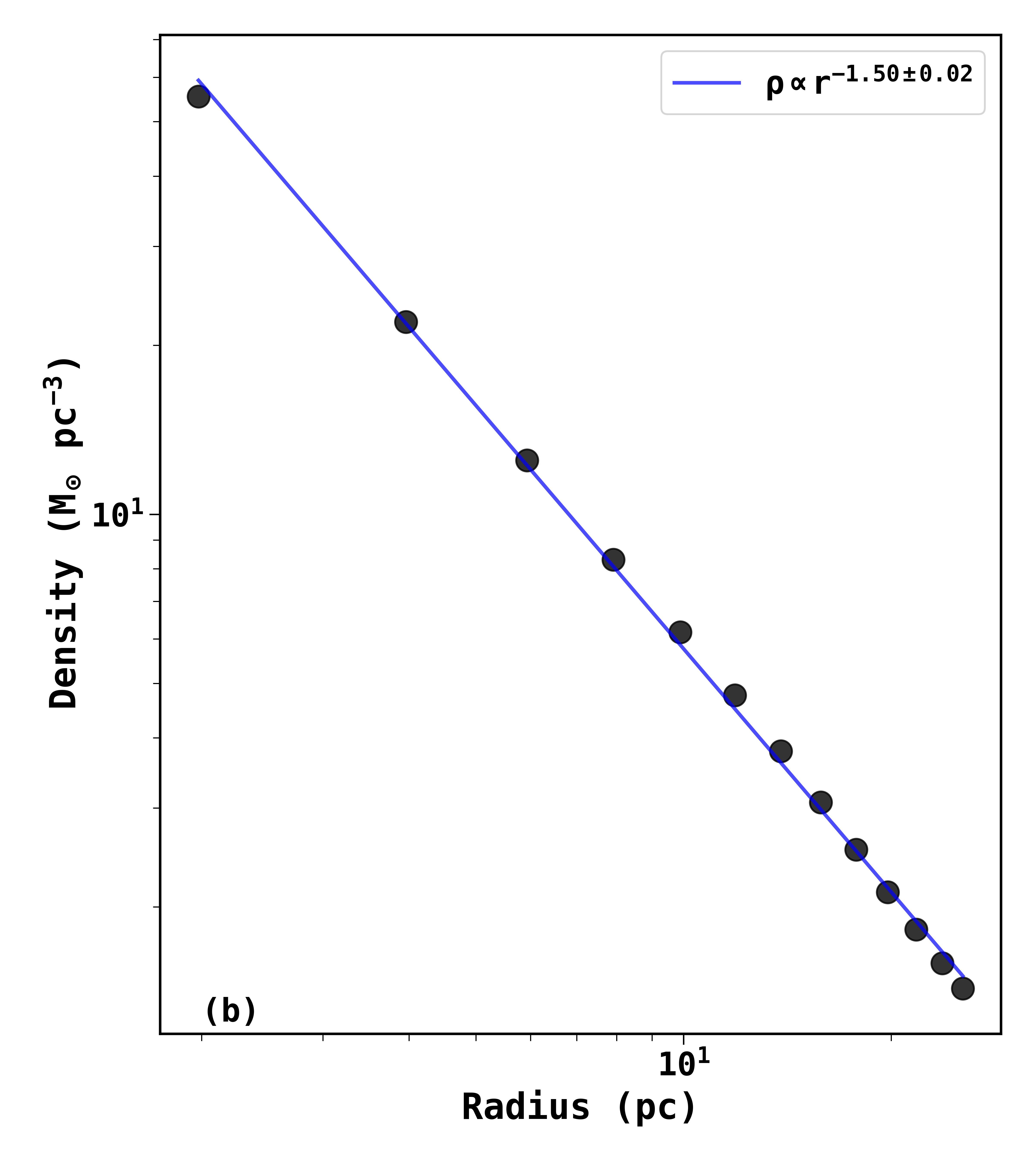
The density profile of a single cloud is also important for theoretical considerations of star formation. For example, it has been suggested that a density profile of the form, (r) r-1.5, is indicative of a self-gravitating spherical cloud supported by turbulence (Murray & Chang 2015, e.g.), while a profile of the form, (r) r-2, is indicative of a gravity dominated system (Donkov & Stefanov 2018; Li 2018; Chen et al. 2021, e.g.). Figure 7b shows the density profile of the G148.24+00.41 cloud along with the best-fitted power-law profile (blue solid line). We find that (r) r-1.5 best fits the overall large-scale structure of the cloud. We note that this is the overall density profile of the cloud, but individual dense pockets of gas or clumpy structures can have a steeper density profile. As G148.24+00.41 is located at 3.4 kpc, unveiling the profile of such structures would require high-resolution observations. However, it is worth mentioning that steeper density profiles with an average power-law index between 1.8 to 2 have been observed in massive star-forming clumps (Garay et al. 2007, e.g.).

3.2.5 Boundness Status of G148.24+00.41
A large reservoir of bound gas is key for making massive clusters because theories and simulations often invoke gas inflow from large scale (Gómez & Vázquez-Semadeni 2014; Padoan et al. 2020, e.g.). However, it is suggested that on relatively short time-scales (typically a few Myr) since its formation, GMCs can be unbound as colliding flows and stellar feedback regulate the internal velocity dispersion of the gas and so prevent global gravitational forces from becoming dominant (Dobbs et al. 2011). So relatively older clouds can be unbound, although it is also suggested that large-scale unbound clouds can also have bound substructures where star cluster formation can take place (Clark & Bonnell 2004; Clark et al. 2005).
Whether a cloud is bound or not is usually addressed by calculating the virial parameter, , which compares the virial mass to the actual mass of the cloud (Bertoldi & McKee 1992). A cloud is bound if 2 and unbound if 2 (Mao, Ostriker, & Kim 2020). It is in gravitational equilibrium if its actual mass and virial mass are equal.
We estimated the virial mass for G148.24+00.41, assuming it is a spherical cloud with a density profile, , and using the equation from MacLaren et al. 1988 in the following rewritten form:
| (2) |
where is the radius of the cloud and is the line-width of the gas. Here, we adopt and = 3.55 0.05 km s-1(see Section 3.1) and assume that describes the average line width of the whole cloud, including the central region. The derived virial mass turns out to be M⊙, while the estimated dust mass is M⊙ (see Section 3.2.1), resulting , and hence the whole cloud is likely bound. This remains true even if we use the lower mass obtained from extinction analysis.

F
3.3 Protostellar Content and Inference from their Distribution
3.3.1 Point Sources and their Evolutionary Status
The satellite offers a unique opportunity to study the earliest phases of stellar sources. In particular, 70 m band is very important for identifying deeply embedded class 0/I objects because it has been found that 70 m is less sensitive to circumstellar extinction and geometry of the disc that significantly affects the 3.6–24 m band. 70 m is also less affected by external heating that becomes effective above 100 m (Dunham et al. 2006).
Figure 8a shows the 70 m image of the G148.24+00.41 cloud. As can be seen, the image displays a significant number of sources distributed roughly in a linear sequence from north-east to south-west, and most of the sources seem to be embedded in high column density material of . Since such high column density regions of a molecular cloud are the sites of recent star formation (André et al. 2010, e.g.), these sources are possibly young protostars of the G148.24+00.41 cloud at their early evolutionary stages.
To understand the nature of the sources, we downloaded the 70 m point source catalogue (Marton et al. 2017; Herschel Point Source Catalogue Working Group et al. 2020) from Vizier (Ochsenbein, Bauer, & Marcout 2000). In total, we retrieve 48 point sources within the cloud radius having SNR 3.0. As noted by Herschel Point Source Catalogue Working Group et al. 2020, the detection limit of the point source catalogue is a complex function of the source flux, photometric band, and the background complexity. We thus look to the reliability of the downloaded point sources by visually inspecting their positions and intensities on the 70 m image. We find that some sources are too faint to be considered as a point source, and also find that a few likely bright sources (which appear to be extended on the image) are also missing in the catalogue. The former could be the artefact due to the non-uniform background level usually found in images, while the latter could be due to the fact that these sources failed to pass the point source quality flags such as confusion and blending flags, implemented in Herschel Point Source Catalogue Working Group et al. 2020 to be called a point source. To check the reliability of the faint sources, we create different unsharp-masked images by subtracting median-filtered images of different windows from the original one (Deharveng et al. 2015, e.g.). Unsharp-masked images are useful to detect faint sources or faint structures that are hidden inside bright backgrounds. We again over-plotted the point sources and found that a few sources are likely false detections, thus, did not use them in this work. After removing likely spurious sources, the total number of point sources is 40, with the faintest being a source of 96 mJy. In Figure 8a, these point sources are marked in cyan circles.
In order to assess the evolutionary status of the point sources, we compared their location in the 70 m flux density versus 160 m to 70 m flux density ratio diagram with that of the well-known protostars of the Orion complex, shown in Figure 9. We took the Orion protostar sample from the Orion Protostar Survey (Furlan et al. 2016, HOPS;). It consists of 330 sources that have 70 m detection, 319 of which have been classified as class 0, class I, or flat-spectrum protostars based on their mid-IR spectral indices and bolometric temperatures, while 11 sources have been classified as class II objects. As can be seen from Figure 9, most of the point sources (red dots) have 160 m to 70 m flux density ratio 1.0 like the HOPS protostars. The only source that shows a relatively smaller ratio with respect to the rest of the sources is the most luminous 70 m source. This source is the most massive YSO in our sample (more discussion in Section 3.3.3 and 3.3.4). To access the degree of contamination that might be present in our sample, in the form of extragalactic sources or other dusty objects along the line of sight, we did a similar analysis for the point sources present in the control field region. We find that none of the control field sources are located in the zones of the HOPS protostars, implying that contamination is negligible and the majority of the identified 70 m point sources in G148.24+00.41 are likely true protostars. The identification of these protostars suggests that, the central area of the cloud is actively forming protostars compared to the rest of the cloud.

3.3.2 Fractal Nature of the Cloud
For clouds and clumps at their early stage of evolution, the distribution of cores or young protostars carries the imprint of the original gas distribution.
We examine the structure of the G148.24+00.41 cloud using identified protostars and implementing the statistical Q-Parameter method (Cartwright & Whitworth 2004), which is based on the minimum spanning tree (MST) technique. A MST is defined as the unique network of straight lines that can connect a set of points without closed loops, such that the sum of all the lengths of these lines (or edges) is the lowest. The Q-Parameter method has been extensively studied in the literature for understanding the clustering (large-scale radial density gradient or small-scale fractal) structure of the star-forming regions and molecular clouds (Schmeja & Klessen 2006; Parker et al. 2014; Sanhueza et al. 2019; Dib & Henning 2019; Sadaghiani et al. 2020, e.g.). Q is expressed by the following equation:
| (3) |
where the parameter is the normalized mean edge length of MST, defined by:
| (4) |
where is the total number of sources, is the length of edge , and is the area of the smallest circle that contains all the sources. The value of represents the correlation length, i.e. mean projected separation of the sources normalized by the cluster radius and is given by
| (5) |
where is the vector position of the point and is the radius corresponding to area A. The decreases more quickly than as the degree of central concentration increases, while decreases more quickly than as the degree of subclustering increases (Cartwright & Whitworth 2004). Therefore, the Q parameter not only quantifies but also differentiates between the radial density gradient and fractal subclustering structure.
Figure 10 shows the MST graph of the protostars in our sample. In the present case, we define the radius as the projected distance from the mean position of all cluster members to the farthest protostar following Schmeja & Klessen 2006. Doing so, we calculated and as 0.27 and 0.41, respectively, which leads to a Q value of . Including the protostars identified by the Star Formation in the Outer Galaxy (SFOG) survey (Winston, Hora, & Tolls 2020), that has used Spitzer-IRAC, WISE, and 2MASS data in the wavelength range 1-22 m, though we improved the statistics of protostars sample to 70, but find that Q-value largely remains the same, i.e. Q 0.62, a change of only 6%.
We note that the normalization to cluster radius makes the Q parameter scale-free, but a small dependence of the number of stars on the Q parameter is found in simulations (Parker 2018, e.g.). This is also seen in our analysis, as we found a change in Q value only by 6%. Apart from the number of stars, the presence of outliers can also significantly affect the Q parameter (Parker & Schoettler 2022). To check the significance of outliers on our Q value, we removed possible outliers from our sample, which are far away from the main star-forming region (i.e. sources located outside the rectangular box shown in Figure 8a; these sources are also located away from the AV 5 mag contour, shown in the right panel of Figure 8b) and did the MST analysis. We found that the Q value changes only by 3%, resulting a total uncertainty of 7% (i.e. Q ) due to the above factors.
We also looked at how the completeness of the 70 m catalogue could affect our Q-value. Since most of the protostars are distributed in the central area of the cloud with AV 5 mag, we estimated the completeness limit of the 70 m catalogue in the central area, i.e. the area roughly enclosing the boundary of the AV 5 mag. We estimated completeness by injecting artificial stars on the 70 m image and performing detection and photometry in the same way as done in the original catalogue (Marton et al. 2017, for details, see). Doing so, we find that our 70 m point source sample in the central area is 80% complete at the flux level of 200 mJy. Recalculating the Q value above the 80% completeness limit, we find the Q value to be around 0.71.
The value of Q 0.8 is interpreted as a smooth and centrally concentrated distribution with volume density distribution , while Q 0.8 is interpreted as clusters with fractal substructure, and Q 0.8 implies uniform number density and no subclustering (see Cartwright & Whitworth 2004, for discussion). Cartwright & Whitworth 2004 drew these inferences by studying the structure of the artificial star clusters, created with a smooth large-scale radial density profile () and with substructures having fractal dimension D, and correlating them with the Q-value. The fractal substructures of various fractal dimensions were generated following the box fractal method of Goodwin & Whitworth 2004. We direct the reader to Goodwin & Whitworth 2004 for the details of the box fractal method. Cartwright & Whitworth 2004 found that Q is correlated with the radial density exponent for Q 0.8, and for fractal clusters, the Q is related to fractal dimension D such that the Q parameter changes from 0.80 to 0.45 as the D changes from 3.0 (no subclustering) to 1.5 (strong subclustering). From the simulation results of Cartwright & Whitworth 2004, we infer that our estimated Q value (i.e. ), corresponds to a notional fractal dimension, D 2.2, which represents a moderately fractal distribution.
Since most of the protostars are distributed in the central area of the cloud, shown in Figure 8. From this analysis, we infer that the cloud in its central area is moderately fractal.
3.3.3 Luminosity of Protostars and their Correlation with the Gas Surface Density


Dunham et al. 2006, using radiative transfer models, demonstrated that 70 m is a crucial wavelength for determining bolometric luminosity (Lbol ) of embedded protostars, as radiative transfer models are strongly constrained by this wavelength, and it is largely unaffected by the details of the source geometry and external heating. Furthermore, Dunham et al. 2008 and Ragan et al. 2012 find that the 70 m flux correlates well with the bolometric luminosity of the low and high-mass protostars, respectively (Elia et al. 2017, see also discussion in ).
We find that a significant number of the 70 m point sources are blended at longer wave bands. Thus, in this work, we used the empirical relation between 70 m flux and Lbol given by Dunham et al. 2008 for estimating Lbol of the protostars:
| (6) |
where is in erg cm-2 s-1, though this way of estimating luminosity is likely accurate within a factor of 2–3 (Commerçon et al. 2012; Samal et al. 2018, e.g.). We estimated the luminosity of the sources keeping this limitation in mind and found that they lies in the range 3–1850 L⊙, with a median value around 12 L⊙.
Figure 11a shows the luminosity distribution of the sources on the mass surface density map, made from the column density map. The uncertainty in the luminosity is due to the uncertainty in the distance of the cloud and the flux of the point sources. As can be seen that the most luminous source (the reddest solid dot) is located in the zone of the highest surface density, and most of the sources are confined to surface density 110 M⊙ pc-2. Figure 11b shows the bolometric luminosity versus peak mass surface density corresponding to the source location. From the figure, one can see that sources are distributed in the surface density range 80–900 M⊙ pc-2 and shows a positive correlation with the mass-surface density, implying that higher luminous sources are found in the higher surface density zones. Figure 11c shows the luminosity distribution of the sources from the location of the cloud’s likely centre of potential. As discussed in Section 3.2.1, the inner region of the cloud is elongated and filamentary, thus, finding its centre of gravitational potential is not easy, so we define the cloud’s gravitational centre as the location of the highest surface density area on the smoothed surface density map (shown in Figure 11a). We made a smoothed map to understand the structure that dominates the large-scale distribution as a function of scale. The highest surface density area on the smoothed map also corresponds to the location of a hub, seen in the SPIRE images (discussed in Section 4.1.3). From Figure 11c, a declining trend of luminosity distribution with the distance from the adopted centre can be seen, although many low-luminosity sources are also located close to the centre along with the most luminous source.
Altogether, the above analyses suggest that although protostars are distributed in a range of surface densities, the luminous sources are located in the highest surface density zones and also close to the cloud’s centre of potential.

3.3.4 Mass Segregation
A higher concentration of massive objects near the cloud or cluster centre compared to that of their low-mass siblings is known as mass-segregation. However, it remains unclear whether mass segregation is primordial or dynamical, particularly in young star-forming regions or cluster-forming clumps. Mass segregation is an important constraint on theories of massive stars and associated cluster formation. For example, it is suggested that cores in the dense central regions of cluster forming clumps can accrete more material than those in the outskirts; therefore, primordial mass segregation would be a natural outcome of massive star formation (Bonnell & Bate 2006; Girichidis et al. 2012). However, it is also suggested that mass segregation can also occur dynamically. In this scenario, massive stars form elsewhere but sink to the centre of the system potential through dynamical interaction with the other members (Allison et al. 2010; Parker et al. 2014; Parker et al. 2016; Domínguez et al. 2017, e.g.).
One way to test the above theories is to look for the distribution of young protostars and cores in young molecular clouds. Because, the velocity dispersion of cores in young star-forming regions is found to be 0.5 km s-1, while the velocity dispersion of the class II sources in the same regions is found to be higher, at around 1 km s-1(Foster et al. 2015, e.g. NGC 1333;). Thus, the class II stars of a star-forming region can travel pc-scale distance in a Myr timescale from their birth locations, while protostars being young (age yr) and often attached to the host core, nearly represent their birth locations.
To quantify the degree of mass-segregation () in star-forming regions, Allison et al. 2009 described a statistical way that uses MST distribution of stars. This method works by comparing the average MST length of the most massive stars of a cluster with the average MST length of a set of the same number of randomly chosen stars and is written as:
| (7) |
For good statistical results, one needs to take a significant number of random samples (Maschberger & Clarke 2011). Here, is the sample mean of average MST lengths of randomly selected stars, is the average MST length of most massive stars, and is the standard deviation of the length of these random stars. The greater than 1 means that the most massive stars are more concentrated compared to a random sample, and therefore, the cluster shows a signature of mass segregation, while implies that the distribution of massive stars is comparable to that of the random stars.
In the present work, we have not estimated the mass of the protostars (typical age 105 yr), however, since luminosity is proportional to the mass (e.g. from the theoretical isochrones of Bressan et al. 2012, we find that for the stars in the mass range 1–10 M⊙ and an age of 105 yr), thus, we considered that any evidence of luminosity segregation is equivalent to mass-segregation. We used only protostars to test the mass-segregation effect, as we have luminosity measurements of only these protostars. We acknowledge that in this simple mass-luminosity relation, we have ignored the role of accretion luminosity on the total luminosity of the protostars, but it is expected to be around 25% for the class I sources (Hillenbrand & White 2004, e.g.).
We calculated starting at N (number of most massive stars) = 5 up to the number of protostars in our sample and calculated by picking 500 random sets of N stars. Figure 12 shows the for increasing values of N. As can be seen, the 8 most massive stars show the maximum value of (i.e. 3.2 0.5) , then progressively decreases and becomes flat beyond 18 most massive stars. The larger is expected for small N due to stochastic effects in choosing the small random sample (Allison et al. 2009). Like for the analysis of the Q parameter, we also estimated the effect of 70 m point source sample completeness on the mass-segregation and found that to be around 2.8, which is though on the lower-side of the measured for the entire cloud but within the error. This analysis tells that the 8 most massive stars of G148.24+00.41 are likely 3 times closer to each other compared to the typical separation of 8 random stars in the region, suggesting that the mass-segregation effect is likely present in G148.24+00.41. These eight most massive stars (L 50 L⊙) of G148.24+00.41 are located within 9 pc from the adopted centre. We discuss the likely cause of the observed mass-segregation in Section 4.1.3. It is worth mentioning that, like here, mass-segregation of cores has been investigated in a few filamentary environments using ALMA observations involving a small number of cores. For example, Plunkett et al. 2018 reported that massive cores of Serpens South are mass segregated with a median of 4. Similarly, Sadaghiani et al. 2020 also find evidence of mass segregation in the filaments of NGC 6334 with value in the range 2–3. However, we note that within the G148.24+00.41 cloud area, the SFOG survey has identified 48 protostars, 31 of which have no counterparts in the 70 m catalogue. These are likely the low-luminosity sources of the cloud beyond the sensitivity limit of the 70 m image. Since the SFOG survey has used data in the wavelength range 1–22 m to identify these protostars, robust estimation of their bolometric luminosity is not possible. We thus refrain from using these sources in the MST analysis, but we acknowledge that the non-inclusion of these protostars and also any embedded low-luminosity protostars that are not detected in the SFOG survey may bias our results. Future high sensitivity multi-band long-wavelength observations are needed for a more precise estimation of the mass segregation.


4 Discussion
The G148.24+00.41 cloud is massive and bound, yet it is still speculative to say whether it will form a high-mass cluster. Here, we consider a cluster with a total stellar mass 104 M⊙ as a massive cluster, following the classification scheme of Portegies Zwart et al. 2010.
Simulations suggest that a high-mass cluster may form: (a) if the cloud collapses to form a centrally condensed massive dense clump, which fragments to form stars at a high efficiency (Banerjee & Kroupa 2015; Banerjee & Kroupa 2018). By doing so, the clump may produce a rich cluster in a short span of time before the stellar feedback commences and the process is called as “monolithic” or “in-situ” mode of cluster formation (Banerjee & Kroupa 2015; Walker et al. 2015, e.g.). In this scenario, the cluster forms at higher initial stellar densities, and then relaxes to its final state after it has expelled the gas.
(b) In the literature, many large-scale dynamical models involving the evolution of molecular clouds over an extended period of time have been proposed for making massive clusters. These include models such as global hierarchical collapse (Vázquez-Semadeni et al. 2019, e.g.), gravitationally-driven gas inflows (Smith, Longmore, & Bonnell 2009, e.g.), and conveyor-belt collapse (Longmore et al. 2014; Walker et al. 2016; Barnes et al. 2019; Krumholz & McKee 2020). All these models have some similarities and differences (Vázquez-Semadeni et al. 2019, for details, see the review article by). Broadly, these models point to the formation, evolution, and coalescence/convergences of substructures within a molecular cloud into a more massive structure driven by global collapse, leading to the formation of massive stars and associated cluster. These models broadly suggest that, while the molecular cloud globally evolves, due to its hierarchical nature, it also simultaneously forms stars at local high-density structures (i.e. within the filaments or dense regions), as their free-fall times are shorter than the free-fall time of the global cloud. And as the evolution of the cloud proceeds, the cold matter in the extended environment and the protostars formed within them can eventually be transported to the remote collapse centre, located at the cloud’s centre of potential. This can occur via filaments, anchored by large-scale global collapse (Pineda et al. 2022; Hacar et al. 2022, for details, see review articles by ), where filaments act like conveyor-belts. In these scenarios, star formation would proceed over several crossing times leading to significant age spread in cluster members, the seeds of massive stars are expected to be located near the cloud’s center of potential, and more younger stars are expected to form in the end. As a consequence, primordial mass segregation is expected, and also, the cloud’s central potential is expected to have more young stars compared to the stars in the extended part of the cloud (Vázquez-Semadeni et al. 2019, e.g., see discussion in).
In the following, we discuss the possible scenarios of massive star and associated cluster formation in G148.24+00.41, and discuss our results in the context of the above cluster formation theories.
4.1 Observational Evidence of Massive Cluster Formation and Processes Involved in G148.24+00.41
4.1.1 Evidence of High-Mass Star and Associated Cluster Formation
Observations suggest that the majority of the massive stars form in clusters (Lada & Lada 2003) and also, the mass of the most massive star of a cluster is proportional to the total mass of the cluster (Weidner, Kroupa, & Bonnell 2010, e.g.). Therefore, the presence of young massive star(s) in a cloud is an indication of ongoing cluster formation. Another way of finding whether or not a cloud would form a high-mass cluster is to look for mass versus radius diagram as it is suggested that to form a high-mass cluster, a reservoir of cold gas concentrated in a relatively small volume is likely required (Bressert et al. 2012; Ginsburg et al. 2012; Urquhart et al. 2013, e.g.).
Based on column density maps derived from dust emission (MAMBO and Bolocam) and extinction (2MASS) data, Kauffmann & Pillai 2010 suggested a criterion for massive star formation. They argued that the clouds known to be forming massive (M M⊙) stars have structural properties described by M⊙, where is the mass within radius . Clouds below this criterion are unlikely to form massive stars. A similar conclusion is also given by Baldeschi et al. 2017 for cold structures to form high-mass stars. In Figure 13, we show these empirical relations along with the location of the G148.24+00.41 cloud corresponding to its total mass and dense gas mass. As can be seen, both the estimates of G148.24+00.41 lies nearly above these relations, suggesting that massive star formation is expected in G148.24+00.41. However, it is worth noting that simulations suggest that the star formation efficiency, though highly dependent on the initial conditions, is usually low at the very initial stages of cloud evolution and accelerates after a few free-fall time (Zamora-Avilés et al. 2012; Lee, Miville-Deschênes, & Murray 2016; Caldwell & Chang 2018; Clark & Whitworth 2021). In addition, models also suggest that compared to low-mass stars, the massive stars form last in a molecular cloud (Vázquez-Semadeni et al. 2009; Vázquez-Semadeni et al. 2019) which is supported by some observations (Foster et al. 2014, e.g.), however, there are also contrasting observational results suggesting that massive stars may form in the early phases of the molecular clouds (Zhang et al. 2015, e.g.).
All the above models point to the fact that the non-detection of high-mass stars in a massive cloud does not imply that it would not form high-mass stars. It may simply be due to the fact that the cloud is at the very early stages of its evolution and has not had enough time to form massive stars. Nonetheless, in the present work, the most luminous 70 m point source of our sample corresponds to a probable massive YSO (MYSO; RA = 03:56:15.36, Dec = +53:52:13.10) listed in the MYSO sample of the Red MSX Source (RMS) survey (Lumsden et al. 2013). Cooper et al. 2013 confirms the YSO nature of the Red MSX Source using near-infrared spectroscopy observations. Scaling the luminosity of the Red MSX massive YSO tabulated in Cooper et al. 2013 to our opted distance, we find its luminosity to be 4200 L⊙ (= ), which is two times of our 70 m flux-based luminosity estimation (see Section 3.3.3). The dynamical age of the MYSO based on the extent and the velocity of the outflow lobes, traced with the CO (J = 3–2) transition, is suggestive of a very young age, around 105 yr (Maud et al. 2015). No UCH ii region has been detected in the 5GHz continuum image of the RMS survey. The typical age of the UCH ii region is around 105 yr. All these results imply that the MYSO is in its early stages of evolution.
Figure 13 also shows the location of young massive stellar clusters (Pfalzner 2009, Mass 5 103 M⊙ and Age 5 Myr; ) by the shaded area. Also shown are the young massive cluster (YMC) precursor clouds of the Galactic disk (Ginsburg et al. 2012; Urquhart et al. 2013) and Galactic Center (Immer et al. 2012; Longmore et al. 2012; Longmore et al. 2013; Walker et al. 2015, GC;). The YMC precursor clouds that have been identified at the Galactic Centre, are mostly quiescent, despite tens of thousands of solar masses of gas and dust within only a few parsecs.
It is believed that massive GC clouds are favourable places for YMC formation. It hosts the two most young massive (mass 104 M⊙) clusters in the Galaxy, the Arches and Quintuplet, which have formed in the GC recently, with ages of 3.5 and 4.8 Myr, respectively (Walker et al. 2018, e.g.). As can be seen from Figure 13, in terms of mass and compactness, compared to Galactic center clouds, the dense gas mass of G148.24+00.41 is lower by an order of magnitude while its radius is higher by a factor of 2–3. In G148.24+00.41, star formation is underway, as evident from the detection of YSOs of various classes, therefore, some of the gas has already been consumed in the process. Even then, comparing the current location of G148.24+00.41 with the location of the YMC progenitor clouds in the disk and GC, it appears that G148.24+00.41 may not form a YMC like the Arches cluster (mass 104 M⊙ and radius 0.5 pc). We compared the mass surface density profile of G148.24+00.41 within 2 pc from the hub center with other Galactic YMC precursor clouds discussed in Walker et al. 2016, and found that the surface density profile of G148.24+00.41 is substantially below all of the Galactic centre clouds, and the extreme cluster forming regions in the disc. This again points to the fact that although G148.24+00.41 has a significant mass reservoir, but it is spread over a larger projected area, hence the lower surface mass density, and lower potential for forming a star cluster like the Arches.
The figure also shows the turbulent pressures for the different environments in our Galaxy (Longmore et al. 2014, for details see). Assuming that G148.24+00.41 is pressure confined by the turbulent pressure of the Galactic disk, to become unbound, the internal pressure of the cloud has to be of the order of 105 K cm-3. The present dynamical status of G148.24+00.41 suggests that it is gravitationally bound. In the following, we explore what kind of cluster G148.24+00.41 may form.
4.1.2 Likely Age and Mass of the Total Embedded Stellar Population
To understand the stellar content of the hidden embedded population, we again make use of the SFOG survey YSO catalogue. In the field of G148.24+00.41, SFOG survey has identified 175 YSOs, out of which 48 are class 0/I, 120 are class II, and 7 are class III sources. We matched and combined the SFOG YSO catalogue with the protostars identified in this work, which resulted in a total of 187 YSOs, out of which 70 are found to be protostars.

Young stellar objects take different amounts of time to progress through the various evolutionary stages. Protostars (Class 0, Class I, and flat-spectrum sources) represent an earlier stage of young stellar object’s evolution than the class II and class III sources, thus, the ratio of protostars to the total number of YSOs (or class II sources) are often used to derive relative ages of the star-forming regions (Jørgensen et al. 2006; Gutermuth et al. 2008; Myers 2012, e.g.). For deriving an approximate age of G148.24+00.41, we compare its protostellar fraction with that of the well-known star-forming regions. Figure 15 shows the protostellar fraction (i.e. ratio of protostars to the total number of protostars plus class II YSOs) vs. age of the 23 star-forming regions tabulated in Myers 2012. In this figure, class III sources are not considered in the total number of YSOs following Myers 2012, as the authors did not consider class III sources in their analysis, arguing that they are incomplete. As can be seen from Figure 15, the protostellar fraction declines with age. Assuming that the protostellar fraction decays exponentially with the age, like the disk fraction in young clusters (Ribas et al. 2014), we fitted the observed protostellar fraction as a function of time using an exponential law of the form: = , where is the age of the sample (in Myr), is the initial protostellar fraction, is the characteristic timescale of decay in protostellar fraction (in Myr), and is a constant level. The best-fitted value of , , and are 0.847 0.022, 0.700 0.024, and 0.093 0.005, respectively. The derived relation is an indication of the fact that the protostar’s life-time is around 0.7 Myr. For G148.24+00.41, we estimated the protostellar fraction to be 37% with an admittedly high uncertainty, which is difficult to quantify considering the likely completeness limits of various bands used in the SFOG survey for identifying the YSOs and also the sensitivity limits of these bands in detecting disk-bearing stars in the cloud due to its distant nature. Nonetheless, taking the observed protostellar fraction a face value and using the above-derived relation, we make a crude assessment of the age of G148.24+00.41 to be roughly around 1 Myr, which we used in this work.
Measuring the mass of individual embedded YSOs is an extremely challenging task in young star-forming clouds due to the presence of variable extinction within the cloud and also the presence of infrared excess in YSOs. Nonetheless, to get a rough census of the total stellar mass that might be embedded in the cloud, we first estimated the typical detection limit of our YSO sample. We do so, by searching the counterparts of the YSOs in UKIDSS near-infrared bands, adopting 1 Myr as their age and assuming a minimum foreground AV of 5 mag (which corresponds to the outer column density boundary of the central area, within which the majority of the YSOs are concentrated) is present in the direction of the YSOs. We find that the typical detection limit is around 0.9 M⊙. Here, we used 1Myr theoretical isochrone from Bressan et al. 2012 and corrected the isochrone for the distance and extinction to compare with the observed near-infrared magnitudes of the YSOs.
The luminosity of the most massive YSO is around 1900 L⊙, which corresponds to a star of 8 M⊙ (Mottram et al. 2011, see Table 1 of). Considering that there are 187 point sources embedded in the cloud between 0.9 and 8 M⊙ and using the functional form of Kroupa mass-function (Kroupa 2001), we estimated the total stellar mass to be 500 M⊙ and extrapolating down to 0.1 M⊙, we find the total mass to be 1000 M⊙. Thus, we expect an embedded population of total stellar mass around 1000 M⊙ to be present in the cloud. We note that applying a higher foreground extinction would give even a higher mass detection limit for YSOs and, thus, a higher total stellar mass.
4.1.3 Hub Filamentary System and Its Implication on Cluster Formation
Figure 14 shows the central area of the cloud at 250 m. In the image, several large-scale filamentary structures (length 5–20 pc) were found to be apparent. These structures are sketched in the figure by the dotted curves and meant only to indicate the possible existence of large-scale filament-like structures. These structures were identified by connecting nearly continuous dust emission structures present in the cloud. A thorough identification of the filaments is beyond the scope of the present work. Future high-dense gas tracer molecular data would be highly valuable for identifying the velocity coherent structures, thus the filaments in the cloud and their properties (Treviño-Morales et al. 2019, e.g.). However, from the present generic sketch, one can see that the central dense location is located at the nexus of six filamentary structures. We find that this central area is host to an embedded cluster, seen in the near-infrared images. The inset image of Figure 14 shows the cluster in the 3.6 m band, and as can be seen, it contains a rich number of near-infrared point sources with massive YSO at its very center. Altogether, the whole morphology of Figure 14 is consistent with the picture of a hub filamentary system put forward by Myers 2009, where several fan-like filaments are expected to intersect, merge and fuel the clump located at their geometric centre (Kumar et al. 2022, e.g. see also discussion in).
As discussed in Section 3.3.4, we have observed the evidence of mass-segregation in the cloud for luminous sources with luminosity 50 L⊙ within 9 pc from the central hub.
This observed mass-segregation could be of primordial or dynamical origin. In case of star clusters, the dynamical origin is primarily driven by the interaction among the stars. In the present case,
the total mass of the embedded population is around
1000 M⊙, which is 3% of the
total gas mass ()
enclosing these YSOs. This is suggestive of the
fact that the gravitational potential
in the central area of the cloud
is dominated by the gas than the stars; thus, dynamical interaction among the stars might not be so effective at this stage of the cloud’s evolution for global mass-segregation to happen. The cold molecular gas and dust are usually thought to impede the process of dynamical interaction.
Next, we look for whether the observed mass-segregation is driven by filamentary flows. Because filaments are often associated with longitudinal flows (Peretto et al. 2013; Dutta et al. 2018; Ryabukhina et al. 2018, e.g.), heading toward the bottom of the potential well of the system (Treviño-Morales et al. 2019, e.g.). We calculated the flow crossing time as: =, where vinf is the flow velocity and R is the distance travelled by gas flow. In the absence of vinf information for G148.24+00.41, we used the typical value of vinf in the range 1–1.5 km s-1pc-1, observed in the large-scale filaments that are radially attached to the massive star-forming hubs (Treviño-Morales et al. 2019; Montillaud et al. 2019, e.g.), to calculate the flow travel distance. Doing so, we estimated that in 0.1–1 Myr of time (i.e. the likely age range of the region; discussed in Sections 4.1.1 and 4.1.2), the flow would travel a distance in the range of 0.15 to 1.5 pc. If this flow carries massive prestellar cores or massive protostars along with it, then one would expect that the effect of mass-segregation within 1.5 pc from the centre of the cloud’s potential may be of flow origin. However, we want to stress that it is very unlikely that the massive prestellar core or protostars would flow along the filaments with the same velocity as gas particles may do. Thus, the aforementioned estimated travel distance would be an upper limit for the protostars.
Since the mass-segregation scale (9 pc) for the massive stars is larger than the flow travel distance (0.15–1.5 pc) for the adopted age range of the system, we thus hypothesized that the evidence of global mass-segregation observed in G148.24+00.41, if confirmed (see possible biases in Section 3.3.4), may suggest towards its primordial origin. Deeper photometric observations along with the velocity measurements of the gas and protostars would shed more light on this issue.
4.1.4 Prospects of Cluster Formation Processes in G148.24+00.41
Simulations suggest that the density profile reflects the physical processes influencing the evolution of a cloud. The overall density profile, , obtained for G148.24+00.41 is a signature of a self-gravitating turbulent cloud. This is also revealed by the distribution of the protostars. We obtained Q-value around 0.66 from the distribution of protostars, suggesting that the central region is moderately fractal with a fractal dimension equivalent to 2.2. This fractal structure could be a consequence of both gravity and turbulence. For example, Dobbs et al. 2005 simulated a turbulent clump of density profile, and found that the clump is able to fragment into hundreds of cores that are tied with filamentary structures. Q-value 0.9 generally represents a steeper density profile of exponent 2. Individual clumps may have a steeper density profile, but the central area as a whole is fractal. In other words, the central area of the cloud is different from the profile that one would expect for a cloud to form a single compact cluster via monolithic collapse. The distribution of protostars across the length of the dense gas over a range of densities (see Section 3.3.3) also disfavours a monolithic mode of cluster formation in G148.24+00.41. Walker et al. 2015; Walker et al. 2016 compared the profile of gas density distribution of the YMC precursor clouds with the stellar density distribution of the YMCs. They found that the density profile of the former is flatter compared to the latter, which led them to suggest that the YMC precursors are not consistent with the monolithic formation scenario of star clusters. Doing a similar analysis, we found that the gas surface density profile of the hub area of G148.24+00.41 is flatter than the stellar distribution of YMCs, supporting the above notion that the present cloud is not centrally concentrated enough to form a typical massive cluster in-situ given the present-day mass distribution.


In Figure 14, we show that the G148.24+00.41 cloud hosts a hub-filamentary system, where cluster formation is happening at the hub of the filaments. The presence of hub-filament systems has also been advocated in flow-driven simulations including global collapse (Smith, Longmore, & Bonnell 2009; Gómez & Vázquez-Semadeni 2014; Vázquez-Semadeni et al. 2019). From the evidence of the hub filamentary system, density profile with a power-law index of 1.5, and low Q-value at the central area, it appears that the whole cloud may be self-gravitating globally. However, at smaller scales, the star formation is occurring in dense structures such as filaments and hubs that are immersed within this large-scale self-gravitating cloud. Moreover, though protostars have formed over a range of densities, the high-luminosity sources (or the high-mass sources) are located around the densest locations of the cloud. We find evidence of mass-segregation in the G148.24+00.41 cloud. The low Q-value and the fact that the flow crossing scale is lesser than the mass-segregation scale suggest that mass segregation is likely primordial. In addition, the massive star, which is still at a very young age, of the order of 105 yr, is found to be located in the central area of the cloud, while the young class II sources whose age lies in the range 1–2 Myr have also been observed in the cloud (Winston, Hora, & Tolls 2020).
Figure 16 shows the distribution of the YSOs on the 250 m image. As can be seen, most of the YSOs are located near the hub or associated filaments. We want to stress that the detection limit of our identified YSOs is around 1 M⊙. Thus, there may be more faint low-mass YSOs distributed in the extended part or diffuse filaments of the cloud and are not identified here. Also, due to the crowding of stellar sources and bright infrared background, the true YSO number identified inside the hub using Spitzer images may be an underestimation. Nonetheless, from the present sample, we calculated the protostellar fraction as a function of distance from the central hub, and is shown in Figure 17. As can be seen, the plot signifies that younger sources show the tendency of being located closer to the cloud centre relative to the class II YSOs. All the above evidence point to the flow-driven modes of cluster formation that are discussed in Section 4. So, we hypothesize that, if the cloud will ultimately form a high-mass cluster, it has to go through global hierarchical convergence and merger of its both gaseous and stellar content as advocated in conveyor-belt type models (Longmore et al. 2014; Walker et al. 2016; Vázquez-Semadeni et al. 2019; Barnes et al. 2019, e.g.). The latter can even occur after no gas is left in the system if the stellar sources are part of a common potential (Howard et al. 2018; Sills et al. 2018; Karam & Sills 2022, e.g.).
4.2 Predictions from Models of Hierarchical Star Cluster Assembly and Merger
Assuming that the cloud will form a high-mass cluster through dynamical processes over an extended period of time (over a few Myr), involving global hierarchical collapse and merger of stars and subgroups, then it is tempting to speculate that what kind of cluster it may form.
Gavagnin et al. 2017 studied the early (up to 2 Myr) dynamical evolution of a turbulent cloud of mass M⊙, radius 5 pc, and 3D velocity dispersion 2.5 km s-1. They found that as the cloud collapses, it forms stars in filaments and extended part of the cloud at a slow rate, but a rich high-mass star cluster emerges from the cloud at the end of the simulation that has some features similar to the massive cluster NGC 6303. In terms of mass, radius, and velocity dispersion, the properties of the simulated cloud are nearly the same as the dense gas properties of G148.24+00.41(see Section 3.2.3), implying that G148.24+00.41 has the potential to build a rich cluster.
From an observational point of view, the emergence of a massive star cluster also seems to be feasible for G148.24+00.41, because its embedded stellar mass is 1000 M⊙, while it still has a high reservoir of bound gas to make more stars. If we go by the hypothesis that it is the dense gas that contributes more to star formation, then using the relation between star formation rate and dense gas mass of Lada et al. 2012:
| (8) |
one could make a rough assessment of the total stellar mass that may emerge from the cloud. The and are the total mass and dense gas fraction of the cloud, respectively. By taking dense gas fraction , total gas mass M⊙ (see Section 3.2.3), and assuming star formation would proceed at a constant rate for another 1 to 2 Myr, we find that a stellar system of total mass in the range 1000–2000 M⊙ may emerge from G148.24+00.41. This prediction is also in line with the recent simulation results of Howard et al. 2018. Howard et al. 2018 follow the evolution of massive GMCs (mass in the range 104–107 M⊙) with feedback on and off. They found that the star clusters emerge from the cloud via a combination of filamentary gas accretion and mergers of less massive clusters, and found a clear relation between the maximum cluster (Mmax) mass and the mass of the host cloud (MGMC). Observations also support this prediction (He et al. 2022, e.g.). Following the prediction of Howard et al. 2018 for feedback on and considering the dense gas mass only as the cloud mass, we find that the dense gas reservoir has the ability to form a cluster of total stellar mass 2000 M⊙.
Combining the embedded stellar mass and the expected stellar mass from the present dense gas reservoir, one would expect a total stellar mass in the range 2000–3000 M⊙ to emerge from this cloud. We note that this is the case, without accreting any additional gas from the extended low-density reservoir beyond the effective radius of the dense gas (i.e. 6 pc). However, considering the fact that molecular clouds are highly dynamical, if the cluster accretes cold gas from the extended reservoir, then the total stellar mass is likely an underestimation.
We want to stress that simulations of cluster-forming clouds have shown that molecular clouds tend to have some degree of fractal structures at their early stages of evolution, as found in G148.24+00.41. But the degree of fractality slowly reduces as the evolution proceeds because gravitational collapse together with stellar dynamical interactions among the stars and the subgroups progressively erase the initial conditions of the cloud and build up a dense and spherical star cluster (Maschberger et al. 2010; Gavagnin et al. 2017; Howard et al. 2018, e.g.). If this happens for G148.24+00.41 in future, where most of the stellar sources segregate to a cluster at the bottom of the potential well, we may expect a centrally condensed massive cluster with Q-value 1, otherwise, it may evolve to a massive association of stars or groups.
Although, these predictions suggest that the cloud has the potential to form a rich cluster in the range 2000–3000 M⊙, yet further studies of the cloud concerning its gas properties and kinematics are necessary for investigating whether the filaments that appear in the dust continuum images are indeed converging and funneling the cold matter to the central potential of the cloud. Thus, would facilitate the formation and emergence of a dense cluster like the ones predicted in the above simulations.
5 Summary and Conclusions
We have studied the global properties and cluster formation potency of the G148.24+00.41 cloud using dust continuum and dust extinction measurements. From both the dust continuum and dust extinction map, we found that the cloud is massive (M 105 M⊙) and has dust temperature 14.5 K, radius 26 pc, and surface mass density 52 M⊙ pc-2. It follows the power-law density profile with index 1.5 and has a virial mass almost half of the total cloud mass, which shows that it is likely bound. By comparing G148.24+00.41 with other galactic molecular clouds, studying its clustering structure, identifying its protostellar content, and inspecting different cluster formation scenarios, we found that:
- 1.
G148.24+00.41 shows high gas mass content, which is comparable to GMCs like Orion-A, Orion-B, and California, and higher than the other nearby molecular clouds. From the dust continuum map, its dense gas fraction was found to be 18%, which is slightly smaller than Orion-A and RCrA molecular clouds, but relatively higher than the other nearby MCs. The mass and effective radius of the cloud follows the Larson’s relation, which is in agreement with the other nearby MCs.
- 2.
We identified 40 protostars based on 70 m data. By including the SFOG survey, the total number of protostars reaches to 70. Using MST analysis over these protostars, we found that the Q value is 0.66, which shows that the clustering structure is moderately fractal or hierarchical.
- 3.
The spatial distribution of protostars shows that most of them are located in the central area of the cloud above N 5 1021 cm-2. And the luminosity distribution shows that the high luminosity sources are relatively closer to the cloud centre and located in high surface density regions compared to low luminosity sources. This indicates the signature of mass segregation in the cloud, and we obtained the degree of mass segregation around 3.2 using MST technique.
- 4.
After including the YSOs identified in the SFOG survey using GLIMPSE360 field, we estimate the likely total mass of the stellar population embedded in the cloud to be around 1000 M⊙, and by including the further star formation from dense gas only, we speculate that G148.24+00.41 has the potential to form a cluster in the mass range of 2000–3000 M⊙.
- 5.
The cloud possesses a hub filamentary system, and a young cluster is seen in NIR at the hub location, along with the MYSO of . Along with the mass segregation, the younger sources are closer to the cloud’s centre of potential than the older ones. These findings, along with the evidence like low Q value and density profile, point towards the possibility of conveyor belt type mode of cluster formation in the G148.24+00.41 cloud.
ACKNOWLEDGEMENT
The research work at Physical Research Laboratory is funded by the Department of Space, Government of India. This work makes use of data obtained from the UKIRT Infrared Deep Sky Survey, obtained using the wide field camera on the United Kingdom Infrared Telescope on Mauna Kea. We thank Stefan Meingast for the discussion on using PNICER algorithm to generate the extinction maps. We acknowledge the Herschel Hi-GAL survey team and ViaLactea project funded by EU carried out at Cardiff University. DKO acknowledges the support of the Department of Atomic Energy, Government of India, under Project Identification No. RTI 4002. We thank Eugenio Schisano for providing the Herschel Hi-Gal column density and dust temperature map of the G148.24+00.41 cloud region. We are thankful to S.N. Longmore for sharing the data of massive molecular clouds, pressure lines, and other critical parameters used in their work to compare them with G148.24+00.41. This research made use of the data from the Milky Way Imaging Scroll Painting (MWISP) project, which is a northern galactic plane CO survey with the PMO-13.7m telescope. We are grateful to all the members of the MWISP working group, particularly the staff members at PMO-13.7m telescope, for their long-term support. MWISP was sponsored by National Key R&D Program of China with grant 2017YFA0402701 and CAS Key Research Program of Frontier Sciences with grant QYZDJ-SSW-SLH047.
Data Availability
We used the NIR, FIR, and CO molecular data from UKIDSS, Herschel, and PMO, respectively, in this work. The UKIDSS and Herschel data are publicly available. The PMO data can be shared by the PMO database on reasonable request. We have also used the GLIMPSE360 data of the SFOG survey, which is publicly available on SFOG Dataverse.
References
- Allison et al. (2009) Allison R. J., Goodwin S. P., Parker R. J., Portegies Zwart S. F., de Grijs R., Kouwenhoven M. B. N., 2009, MNRAS, 395, 1449.
- Allison et al. (2010) Allison, R. J., Goodwin, S. P., Parker, R. J., Portegies Zwart, S. F., & de Grijs, R. 2010, MNRAS, 407, 1098.
- André et al. (2010) André, P., Men’shchikov, A., Bontemps, S., et al. 2010, A&A, 518, L102.
- André et al. (2014) André, P., Di Francesco, J., Ward-Thompson, D., et al. 2014, in Protostars and Planets VI, ed. H. Beuther et al. (Tucson, AZ; Univ. Arizona Press), 27.
- André et al. (2016) André P., Könyves V., Roy A., Arzoumanian D., 2016, IAUFM, 29B, 708.
- Baldeschi et al. (2017) Baldeschi A., Elia D., Molinari S., Pezzuto S., Schisano E., Gatti M., Serra A., et al., 2017, MNRAS, 466, 3682.
- Banerjee & Kroupa (2015) Banerjee, S. & Kroupa, P. 2015, MNRAS, 447, 728.
- Banerjee & Kroupa (2018) Banerjee, S. & Kroupa, P. 2018, The Birth of Star Clusters, 424, 143.
- Barentsen et al. (2014) Barentsen, G., Farnhill, H. J., Drew, J. E., et al. 2014, MNRAS, 444, 3230.
- Bressert et al. (2012) Bressert, E., Ginsburg, A., Bally, J., et al. 2012, ApJ, 758, L28.
- Barnes et al. (2019) Barnes A. T., Longmore S. N., Avison A., Contreras Y., Ginsburg A., Henshaw J. D., Rathborne J. M., et al., 2019, MNRAS, 486, 283.
- Battersby et al. (2011) Battersby C., Bally J., Ginsburg A., Bernard J.-P., Brunt C., Fuller G. A., Martin P., et al., 2011, A&A, 535, A128.
- Bertoldi & McKee (1992) Bertoldi F., McKee C. F., 1992, ApJ, 395, 140.
- Bohlin et al. (1978) Bohlin, R. C., Savage, B. D., & Drake, J. F. 1978, ApJ, 224, 13233.
- Bonnell & Bate (2006) Bonnell I. A., Bate M. R., 2006, MNRAS, 370, 488.
- Bressan et al. (2012) Bressan, A., Marigo, P., Girardi, L., et al. 2012, MNRAS, 427, 127.
- Burkert & Hartmann (2004) Burkert, A., & Hartmann, L. 2004, ApJ, 616, 288
- Caldwell & Chang (2018) Caldwell S., Chang P., 2018, MNRAS, 474, 4818.
- Cambrésy (1999) Cambrésy L., 1999, A&A, 345, 965
- Cartwright & Whitworth (2004) Cartwright A., Whitworth A. P., 2004, MNRAS, 348, 589.
- Chapman et al. (2009) Chapman N. L., Mundy L. G., Lai S.-P., Evans N. J., 2009, ApJ, 690, 496.
- Chen et al. (2021) Chen, Y., Li, H., & Vogelsberger, M. 2021, MNRAS, 502, 6157.
- Chevance et al. (2022) Chevance, M., Krumholz, M. R., McLeod, A. F., et al. 2022, arXiv:2203.09570.
- Clark & Bonnell (2004) Clark P. C., Bonnell I. A., 2004, MNRAS, 347, L36.
- Clarke & Whitworth (2015) Clarke S. D., Whitworth A. P., 2015, MNRAS, 449, 1819.
- Clark & Whitworth (2021) Clark, P. C. & Whitworth, A. P. 2021, MNRAS, 500, 1697.
- Clark et al. (2005) Clark P. C., Bonnell I. A., Zinnecker H., Bate M. R., 2005, MNRAS, 359, 809.
- Commerçon et al. (2012) Commerçon B., Launhardt R., Dullemond C., Henning T., 2012, A&A, 545, A98.
- Cooper et al. (2013) Cooper, H. D. B., Lumsden, S. L., Oudmaijer, R. D., et al. 2013, MNRAS, 430, 1125.
- Deharveng et al. (2012) Deharveng, L., Zavagno, A., Anderson, L. D., et al. 2012, A&A, 546, A74.
- Dame, Hartmann, & Thaddeus (2001) Dame T. M., Hartmann D., Thaddeus P., 2001, ApJ, 547, 792.
- Deharveng et al. (2015) Deharveng, L., Zavagno, A., Samal, M. R., et al. 2015, A&A, 582, A1.
- Dib & Henning (2019) Dib S., Henning T., 2019, A&A, 629, A135.
- Dobashi (2011) Dobashi K., 2011, PASJ, 63, S1.
- Dobashi et al. (2005) Dobashi K., Uehara H., Kandori R., Sakurai T., Kaiden M., Umemoto T., Sato F., 2005, PASJ, 57, S1.
- Dobbs et al. (2005) Dobbs, C. L., Bonnell, I. A., & Clark, P. C. 2005, MNRAS, 360, 2.
- Dobbs et al. (2011) Dobbs, C. L., Burkert, A., & Pringle, J. E. 2011, MNRAS, 413, 2935.
- Domínguez et al. (2017) Domínguez R., Fellhauer M., Blaña M., Farias J. P., Dabringhausen J., 2017, MNRAS, 472, 465.
- Donkov & Stefanov (2018) Donkov, S. & Stefanov, I. Z. 2018, MNRAS, 474, 5588.
- Dunham et al. (2006) Dunham M. M., Evans N. J., Bourke T. L., Dullemond C. P., Young C. H., Brooke T. Y., Chapman N., et al., 2006, ApJ, 651, 945.
- Dunham et al. (2008) Dunham M. M., Crapsi A., Evans N. J., Bourke T. L., Huard T. L., Myers P. C., Kauffmann J., 2008, ApJS, 179, 249.
- Dutta et al. (2018) Dutta, S., Mondal, S., Samal, M. R., & Jose, J. 2018, ApJ, 864, 154.
- Elia et al. (2017) Elia, D., Molinari, S., Schisano, E., et al. 2017, MNRAS, 471, 100
- Evans et al. (2009) Evans, N. J., II, Dunham, M. M., Jørgensen, J. K., et al. 2009, ApJS, 181, 321.
- Evans et al. (2014) Evans, N. J., II, Heiderman, A., & Vutisalchavakul, N. 2014, ApJ, 782, 114.
- Foster et al. (2015) Foster, J. B. and 16 colleagues 2015. IN-SYNC. II. Virial Stars from Subvirial Cores—the Velocity Dispersion of Embedded Pre-main-sequence Stars in NGC 1333. The Astrophysical Journal 799.
- Foster et al. (2014) Foster J. B., Arce H. G., Kassis M., Sanhueza P., Jackson J. M., Finn S. C., Offner S., et al., 2014, ApJ, 791, 108.
- Furlan et al. (2016) Furlan E., Fischer W. J., Ali B., Stutz A. M., Stanke T., Tobin J. J., Megeath S. T., et al., 2016, ApJS, 224, 5.
- Garay et al. (2007) Garay, G., Mardones, D., Brooks, K. J., et al. 2007, ApJ, 666, 309.
- Gavagnin et al. (2017) Gavagnin, E., Bleuler, A., Rosdahl, J., & Teyssier, R. 2017, MNRAS, 472, 4155.
- Geen et al. (2015) Green, S., Hennebelle, P., Tremblin, P., et al. 2015, MNRAS, 454, 4484.
- Geen et al. (2016) Geen, S., Hennebelle, P., Tremblin, P., et al. 2016, MNRAS, 463, 3129.
- Giannetti et al. (2017) Giannetti A., Leurini S., König C., Urquhart J. S., Pillai T., Brand J., Kauffmann J., et al., 2017, A&A, 606, L12.
- Ginsburg et al. (2012) Ginsburg A., Bressert E., Bally J., Battersby C., 2012, ApJL, 758, L29.
- Girichidis et al. (2012) Girichidis P., Federrath C., Banerjee R., Klessen R. S., 2012, MNRAS, 420, 613.
- Goodwin & Whitworth (2004) Goodwin, S. P. & Whitworth, A. P. 2004, A&A, 413, 929. doi:10.1051/0004-6361:20031529
- Gutermuth et al. (2008) Gutermuth, R. A., Bourke, T. L., Allen, L. E., et al. 2008, ApJ, 673, L151.
- Gómez & Vázquez-Semadeni (2014) Gómez, G. C. & Vázquez-Semadeni, E. 2014, ApJ, 791, 124.
- Hacar et al. (2022) Hacar A., Clark S., Heitsch F., Kainulainen J., Panopoulou G., Seifried D., Smith R., 2022, arXiv, arXiv:2203.09562.
- He et al. (2022) He, H., Wilson, C., Brunetti, N., et al. 2022, ApJ, 928, 57.
- Heiderman et al. (2010) Heiderman, A., Evans, N. J., II, Allen, L. E., Huard, T., & Heyer, M. 2010, ApJ, 723, 1019.
- Heigl, Hoemann, & Burkert (2022) Heigl S., Hoemann E., Burkert A., 2022, MNRAS.tmp.
- Heitsch et al. (2008) Heitsch, F., Hartmann, L. W., Slyz, A. D., Devriendt, J. E.G. & Burkert, A. 2008, ApJ, 674, 316
- Henshaw et al. (2022) Henshaw J. D., Barnes A. T., Battersby C., Ginsburg A., Sormani M. C., Walker D. L., 2022, arXiv, arXiv:2203.11223
- Herschel Point Source Catalogue Working Group et al. (2020) Herschel Point Source Catalogue Working Group, Marton G., Calzoletti L., Perez Garcia A. M., Kiss C., Paladini R., Altieri B., et al., 2020, yCat, VIII/106.
- Heyer et al. (2009) Heyer, M., Krawczyk, C., Duval, J., & Jackson, J. M. 2009, ApJ, 699, 1092.
- Hillenbrand & White (2004) Hillenbrand L. A., White R. J., 2004, ApJ, 604, 741.
- Hoemann, Heigl, & Burkert (2022) Hoemann E., Heigl S., Burkert A., 2022, arXiv, arXiv:2203.07002
- Howard et al. (2018) Howard, C. S., Pudritz, R. E., & Harris, W. E. 2018, Nature Astronomy, 2, 725.
- Immer et al. (2012) Immer K., Schuller F., Omont A., Menten K. M., 2012, A&A, 537, A121.
- Jørgensen et al. (2006) Jørgensen, J. K., Harvey, P. M., Evans, N. J., et al. 2006, ApJ, 645, 1246.
- Karam & Sills (2022) Karam, J. & Sills, A. 2022, MNRAS, 513, 6095.
- Kauffmann & Pillai (2010) Kauffmann J., Pillai T., 2010, ApJL, 723, L7.
- Kauffmann et al. (2008) Kauffmann J., Bertoldi F., Bourke T. L., Evans N. J., Lee C. W., 2008, A&A, 487, 993.
- Kim et al. (2018) Kim, J.-G., Kim, W.-T., & Ostriker, E. C. 2018, ApJ, 859, 68.
- Könyves et al. (2015) Könyves V., André P., Men’shchikov A., Palmeirim P., Arzoumanian D., Schneider N., Roy A., et al., 2015, A&A, 584, A91.
- Krause et al. (2020) Krause, M. G. H., Offner, S. S. R., Charbonnel, C., et al. 2020, Space Sci. Rev., 216, 64.
- Kroupa (2001) Kroupa P., 2001, MNRAS, 322, 231.
- Krumholz, Dekel, & McKee (2012) Krumholz M. R., Dekel A., McKee C. F., 2012, ApJ, 745, 69.
- Krumholz & McKee (2020) Krumholz M. R., McKee C. F., 2020, MNRAS, 494, 624.
- Krumholz & McKee (2020) Krumholz, M. R. & McKee, C. F. 2020, MNRAS, 494, 624.
- Kumar et al. (2022) Kumar, M. S. N., Arzoumanian, D., Men’shchikov, A., et al. 2022, A&A, 658, A114.
- Lada et al. (2012) Lada, C. J., Forbrich, J., Lombardi, M., & Alves, J. F. 2012, ApJ, 745, 190.
- Lada & Lada (2003) Lada, C. J., & Lada, E. A. 2003, ARA&A, 41, 57.
- Lada, Lombardi, & Alves (2010) Lada C. J., Lombardi M., Alves J. F., 2010, ApJ, 724, 687.
- Lada & Dame (2020) Lada C. J., Dame T. M., 2020, ApJ, 898, 3.
- Larson (1981) Larson R. B., 1981, MNRAS, 194, 809.
- Lawrence et al. (2007) Lawrence, A., Warren, S. J., Almaini, O., et al. 2007, MNRAS, 379, 1599.
- Lee, Miville-Deschênes, & Murray (2016) Lee E. J., Miville-Deschênes M.-A., Murray N. W., 2016, ApJ, 833, 229.
- Li (2018) Li, G.-X. 2018, MNRAS, 477, 4951.
- Lombardi et al. (2010) Lombardi, M., Alves, J., & Lada, C. J. 2010, A&A, 519, L7.
- Lombardi et al. (2013) Lombardi, M., Lada, C. J., & Alves, J. 2013, A&A, 559, A90.
- Lombardi et al. (2014) Lombardi, M., Bouy, H., Alves, J., & Lada, C. J. 2014, A&A, 566, A45.
- Longmore et al. (2014) Longmore, S. N., Kruijssen, J. M. D., Bastian, N., et al. 2014, Protostars and Planets VI, 291.
- Longmore et al. (2013) Longmore S. N., Kruijssen J. M. D., Bally J., Ott J., Testi L., Rathborne J., Bastian N., et al., 2013, MNRAS, 433, L15.
- Longmore et al. (2012) Longmore S. N., Rathborne J., Bastian N., Alves J., Ascenso J., Bally J., Testi L., et al., 2012, ApJ, 746, 117.
- Lucas et al. (2008) Lucas P. W., Hoare M. G., Longmore A., Schröder A. C., Davis C. J., Adamson A., Bandyopadhyay R. M., et al., 2008, MNRAS, 391, 136.
- Lumsden et al. (2013) Lumsden, S. L., Hoare, M. G., Urquhart, J. S., et al. 2013, ApJS, 208, 11.
- MacLaren et al. (1988) MacLaren, I., Richardson, K. M., & Wolfendale, A. W. 1988, ApJ, 333, 821.
- Mao, Ostriker, & Kim (2020) Mao S. A., Ostriker E. C., Kim C.-G., 2020, ApJ, 898, 52.
- Marsh et al. (2015) Marsh, K. A., Whitworth, A. P., & Lomax, O. 2015, MNRAS, 454, 428.
- Marsh et al. (2017) Marsh, K. A., Whitworth, A. P., Lomax, O., et al. 2017, MNRAS, 471, 2730.
- Marsh & Whitworth (2019) Marsh, K. A. & Whitworth, A. P. 2019, MNRAS, 483, 352.
- Marton et al. (2017) Marton G., Calzoletti L., Perez Garcia A. M., Kiss C., Paladini R., Altieri B., Sanchez Portal M., et al., 2017, arXiv, arXiv:1705.05693.
- Maschberger & Clarke (2011) Maschberger T., Clarke C. J., 2011, MNRAS, 416, 541.
- Maschberger et al. (2010) Maschberger, T., Clarke, C. J., Bonnell, I. A., et al. 2010, MNRAS, 404, 1061.
- Maud et al. (2015) Maud, L. T., Moore, T. J. T., Lumsden, S. L., et al. 2015, MNRAS, 453, 645.
- Meingast, Lombardi, & Alves (2017) Meingast S., Lombardi M., Alves J., 2017, A&A, 601, A137.
- Miville-Deschênes et al. (2017) Miville-Deschênes, M.-A., Murray, N., & Lee, E. J. 2017, ApJ, 834, 57.
- Molinari et al. (2010a) Molinari S., Swinyard B., Bally J., Barlow M., Bernard J.-P., Martin P., Moore T., et al., 2010, A&A, 518, L100.
- Montillaud et al. (2019) Montillaud, J., Juvela, M., Vastel, C., et al. 2019, A&A, 631, A3.
- Mottram et al. (2011) Mottram J. C., Hoare M. G., Davies B., Lumsden S. L., Oudmaijer R. D., Urquhart J. S., Moore T. J. T., et al., 2011, ApJL, 730, L33.
- Murray & Chang (2015) Murray, N., & Chang, P. 2015, ApJ, 804, 44.
- Myers (2009) Myers, P. C. 2009, ApJ, 700, 1609.
- Myers (2012) Myers P. C., 2012, ApJ, 752, 9.
- Ochsenbein, Bauer, & Marcout (2000) Ochsenbein F., Bauer P., Marcout J., 2000, A&AS, 143, 23.
- Padoan et al. (2020) Padoan P., Pan L., Juvela M., Haugbølle T., Nordlund Å., 2020, ApJ, 900, 82.
- Parker et al. (2014) Parker R. J., Wright N. J., Goodwin S. P., Meyer M. R., 2014, MNRAS, 438, 620.
- Parker et al. (2016) Parker, R. J., Goodwin, S. P., Wright, N. J., et al. 2016, MNRAS, 459, L119.
- Parker (2018) Parker R. J., 2018, MNRAS, 476, 617.
- Parker & Schoettler (2022) Parker R. J., Schoettler C., 2022, MNRAS, 510, 1136.
- Peretto et al. (2013) Peretto, N., Fuller, G. A., Duarte-Cabral, A., et al. 2013, A&A, 555, A112.
- Pfalzner (2009) Pfalzner S., 2009, A&A, 498, L37.
- Pineda et al. (2022) Pineda, J. E., Arzoumanian, D., André, P., et al. 2022, arXiv:2205.03935.
- Planck Collaboration et al. (2011) Planck Collaboration, Ade, P. A. R., Aghanim, N., et al. 2011, A&A, 536, A1.
- Planck Collaboration et al. (2011) Planck Collaboration, Ade, P. A. R., Aghanim, N., et al. 2011, A&A, 536, A7.
- Plunkett et al. (2018) Plunkett A. L., Fernández-López M., Arce H. G., Busquet G., Mardones D., Dunham M. M., 2018, A&A, 615, A9.
- Pon et al. (2012) Pon A., Toalá J. A., Johnstone D., Vázquez-Semadeni E., Heitsch F., Gómez G. C., 2012, ApJ, 756, 145.
- Portegies Zwart et al. (2010) Portegies Zwart, S. F., McMillan, S. L. W., & Gieles, M. 2010, ARA&A, 48, 431.
- Ragan et al. (2012) Ragan S., Henning T., Krause O., Pitann J., Beuther H., Linz H., Tackenberg J., et al., 2012, A&A, 547, A49.
- Reid et al. (2019) Reid M. J., Menten K. M., Brunthaler A., Zheng X. W., Dame T. M., Xu Y., Li J., et al., 2019, ApJ, 885, 131.
- Ribas et al. (2014) Ribas Á., Merín B., Bouy H., Maud L. T., 2014, A&A, 561, A54.
- Rieke & Lebofsky (1985) Rieke, G. H., & Lebofsky, M. J. 1985, ApJ, 288, 618.
- Ryabukhina et al. (2018) Ryabukhina, O. L., Zinchenko, I. I., Samal, M. R., et al. 2018, Research in Astronomy and Astrophysics, 18, 095.
- Sadaghiani et al. (2020) Sadaghiani M., Sánchez-Monge Á., Schilke P., Liu H. B., Clarke S. D., Zhang Q., Girart J. M., et al., 2020, A&A, 635, A2.
- Samal et al. (2018) Samal M. R., Chen W. P., Takami M., Jose J., Froebrich D., 2018, MNRAS, 477, 4577.
- Sanhueza et al. (2017) Sanhueza P., Jackson J. M., Zhang Q., Guzmán A. E., Lu X., Stephens I. W., Wang K., et al., 2017, ApJ, 841, 97.
- Sanhueza et al. (2019) Sanhueza P., Contreras Y., Wu B., Jackson J. M., Guzmán A. E., Zhang Q., Li S., et al., 2019, ApJ, 886, 102.
- Schmeja & Klessen (2006) Schmeja S., Klessen R. S., 2006, A&A, 449, 151.
- Schisano et al. (2020) Schisano E., Molinari S., Elia D., Benedettini M., Olmi L., Pezzuto S., Traficante A., et al., 2020, MNRAS, 492, 5420.
- Sills et al. (2018) Sills, A., Rieder, S., Scora, J., et al. 2018, MNRAS, 477, 1903.
- Smith, Longmore, & Bonnell (2009) Smith R. J., Longmore S., Bonnell I., 2009, MNRAS, 400, 1775.
- Solomon et al. (1987) Solomon, P. M., Rivolo, A. R., Barrett, J., & Yahil, A. 1987, ApJ, 319, 730.
- Spilker et al. (2021) Spilker, A., Kainulainen, J., & Orkisz, J. 2021, A&A, 653, A63.
- Su et al. (2019) Su, Y., Yang, J., Zhang, S., et al. 2019, ApJS, 240, 9.
- Treviño-Morales et al. (2019) Treviño-Morales, S. P., Fuente, A., Sánchez-Monge, Á., et al. 2019, A&A, 629, A81.
- Urquhart et al. (2008) Urquhart J. S., Busfield A. L., Hoare M. G., Lumsden S. L., Oudmaijer R. D., Moore T. J. T., Gibb A. G., et al., 2008, A&A, 487, 253.
- Urquhart et al. (2013) Urquhart J. S., Thompson M. A., Moore T. J. T., Purcell C. R., Hoare M. G., Schuller F., Wyrowski F., et al., 2013, MNRAS, 435, 400.
- Vázquez-Semadeni et al. (2009) Vázquez-Semadeni, E., Gómez, G. C., Jappsen, A.-K., Ballesteros-Paredes, J., & Klessen, R. S. 2009, ApJ, 707, 1023.
- Vázquez-Semadeni et al. (2019) Vázquez-Semadeni, E., Palau, A., Ballesteros-Paredes, J., et al. 2019, MNRAS, 490, 3061.
- Walker et al. (2015) Walker, D. L., Longmore, S. N., Bastian, N., et al. 2015, MNRAS, 449, 715.
- Walker et al. (2016) Walker D. L., Longmore S. N., Bastian N., Kruijssen J. M. D., Rathborne J. M., Galván-Madrid R., Liu H. B., 2016, MNRAS, 457, 4536.
- Walker et al. (2018) Walker D. L., Longmore S. N., Zhang Q., Battersby C., Keto E., Kruijssen J. M. D., Ginsburg A., et al., 2018, MNRAS, 474, 2373.
- Weidner, Kroupa, & Bonnell (2010) Weidner C., Kroupa P., Bonnell I. A. D., 2010, MNRAS, 401, 275.
- Weisz et al. (2015) Weisz, D. R., Johnson, L. C., Foreman-Mackey, D., et al. 2015, ApJ, 806, 198.
- Wenger et al. (2018) Wenger, T. V., Balser, D. S., Anderson, L. D., et al. 2018, ApJ, 856, 52.
- Whitney & GLIMPSE360 Team (2009) Whitney B., GLIMPSE360 Team, 2009, AAS
- Winston, Hora, & Tolls (2020) Winston E., Hora J. L., Tolls V., 2020, AJ, 160, 68.
- Wouterloot & Brand (1989) Wouterloot J. G. A., Brand J., 1989, LNP, 97.
- Yang et al. (2002) Yang, J., Jiang, Z., Wang, M., Ju, B., & Wang, H. 2002, ApJS, 141, 157.
- Yuan et al. (2016) Yuan, J., Wu, Y., Liu, T., et al. 2016, ApJ, 820, 37.
- Zamora-Avilés et al. (2012) Zamora-Avilés, M., Vázquez-Semadeni, E., & Colín, P. 2012, ApJ, 751, 77.
- Zari et al. (2016) Zari, E., Lombardi, M., Alves, J., Lada, C. J., & Bouy, H. 2016, A&A, 587, A106.
- Zhang et al. (2015) Zhang Q., Wang K., Lu X., Jiménez-Serra I., 2015, ApJ, 804, 141.
- Zhang et al. (2018) Zhang, C.-P., Liu, T., Yuan, J., et al. 2018, ApJS, 236, 49.
*