A Neurosymbolic Approach to the Verification of Temporal Logic Properties of Learning enabled Control Systems

Navid Hashemi Affiliation: University of Southern California, Los Angeles CA, USA Bardh Hoxha Affiliation: Toyota Research Institute North America, Ann Arbor, MI, USA E-mail jdeshmuk@usc.edu Tomoya Yamaguchi Affiliation: Toyota Research Institute North America, Ann Arbor, MI, USA E-mail jdeshmuk@usc.edu Danil Prokhorov Affiliation: Toyota Research Institute North America, Ann Arbor, MI, USA E-mail jdeshmuk@usc.edu Geogios Fainekos Affiliation: Toyota Research Institute North America, Ann Arbor, MI, USA E-mail jdeshmuk@usc.edu Jyotirmoy Deshmukh Affiliation: University of Southern California, Los Angeles CA, USA

Abstract

Signal Temporal Logic (STL) has become a popular tool for expressing formal requirements of Cyber-Physical Systems (CPS). The problem of verifying STL properties of neural network-controlled CPS remains a largely unexplored problem. In this paper, we present a model for the verification of Neural Network (NN) controllers for general STL specifications using a custom neural architecture where we map an STL formula into a feed-forward neural network with ReLU activation. In the case where both our plant model and the controller are ReLU-activated neural networks, we reduce the STL verification problem to reachability in ReLU neural networks. We also propose a new approach for neural network controllers with general activation functions; this approach is a sound and complete verification approach based on computing the Lipschitz constant of the closed-loop control system. We demonstrate the practical efficacy of our techniques on a number of examples of learning-enabled control systems.

Keywords:

Signal Temporal Logic, Verification, Deep Neural Network, Lipstchitz constant, Reachability, Model, Controller,

\mathbf{ReLU}

1 Introduction

Learning-enabled components (LECs) offer the promise of data-driven control, and hence they are becoming popular in many Cyber-physical system, CPS, applications. Among LECs, controllers trained using deep learning are becoming popular due to the advances in techniques like deep reinforcement learning and deep imitation learning. On one hand, the use of such LECs has the potential of achieving human level decision making in tasks like autonomous driving, aircraft collision avoidance, and control for aerial vehicles. On the other hand, the use of deep neural network (DNN)-based controllers raises serious concerns of safety.

Reasoning about DNNs is a challenge because DNNs are highly nonlinear [41], and due to the nature of data-driven control, the behavior of a DNN controller at a previously unseen state can be difficult to predict [30]. To address this challenge, there has been significant research on verification for DNNs. Broadly, there are two categories of verification methods; the first category considers DNN controllers in isolation and reasons about properties such as input-output robustness [13, 22, 25], range analysis [12], symbolic constraint propagation through DNNs [29], and overapproximate reachable set computation for DNNs [43]. The second category of methods reasons about DNN controllers in closed-loop with a dynamical model of the environment/plant [12, 21, 20, 23].

In this paper, we also address the closed-loop verification problem. In this problem, we are typically provided with a set of inital states and a set of unsafe states for the system, and the goal is to prove that starting from an arbitrary initial state, no system behavior ever reaches a state in the unsafe set. However, we extend this problem in a significant manner. First, we assume that the desired behavior of the closed-loop system is specified as a bounded horizon Signal Temporal Logic (STL) [33] formula. Second, in contrast to most existing closed-loop verification methods that typically assume that an analytic representation of the system dynamics exists, we allow the system dynamics themselves to be represented as a DNN. Such a setting is quite common in techniques such as model-based deep reinforcement learning [6, 7]. This crucially allows us to reason about systems where the analytic representation of the system dynamics may not be available.

The central idea in our paper is a neurosymbolic verification approach: we reformulate the robust satisfaction (referred to as robustness) of an STL formula w.r.t. a given trajectory as a feed-forward neural network with $\mathbf{ReLU}$ activation functions. We call this transformation $\mathsf{STL2NN}$ . We show that the output of $\mathsf{STL2NN}$ is positive iff the STL formula is satisfied by the trajectory. We note that the verification problem only requires establishing that the given closed-loop dynamical system satisfies a given STL specification. However, by posing the verification problem as that of checking robust satisfaction, it allows us to conclude that the given DNN controller robustly satisfies the given specification.

We then show that when the DNN-controller uses $\mathbf{ReLU}$ activation functions, the problem of closed-loop STL verification can be reduced to computing the reachable set for a $\mathbf{ReLU}$ -DNN. If the controller is not a $\mathbf{ReLU}$ neural network, we propose a technique called Lip-Verify based on computing the Lipschitz constant of the robustness of the given STL formula (as a function of the initial state).

To summarize, the main contributions in this paper are:

1.

We formulate a neuro-symbolic approach for the closed-loop verification of a DNN-controlled dynamical system against an STL-based specification by converting the given bounded horizon specification into a feed-forward $\mathbf{ReLU}$ -based DNN that we call $\mathsf{STL2NN}$ .
2.

For data-driven plant models using $\mathbf{ReLU}$ activation and $\mathbf{ReLU}$ -activation based DNN-controllers, we show that the verification of arbitrary bounded horizon STL properties can be reduced to computing the reach set of the composition of the plant and controller DNNs with $\mathsf{STL2NN}$ .
3.

For arbitrary nonlinear plant models¹¹ 1 In the experimental results, we focus on linear and DNN plant models, but our method is applicable to other nonlinear plant models as well. and DNN-controllers using arbitrary activation functions, we compute Lipschitz constant of the function composition of the system dynamics with STL robustness, and use this to provide a sound verification result using systematic sampling.

The rest of this paper is as follows. In Section 2, we present the background, primary concepts with STL semantics and problem definition. In Section 3, we present the steps to characterize $\mathsf{STL2NN}$ . In Section 4 we classify the verification problem based on the involved activation functions and propose a verification method for each class. We also introduce a structure for formulation of verification problems and introduce our verification toolbox. Finally, we present several case studies and experimental results for our verification methods in Sections 4.3 and 5.1. We conclude with a discussion on related works in Section 6.

2 Preliminaries

In this section, we first provide the mathematical notation and terminology to formulate the problem definition. We use bold letters to indicate vectors and vector-valued functions, and calligraphic letters to denote sets. We assume that the reader is familiar with feedforward neural networks, see [17] for a brief review.

Neural Network Controlled Dynamical Systems (NNCS). Let $\mathbf{s}$ and $\mathbf{u}$ respectively denote the state and input control variables that take values from compact sets $\mathcal{S}\subseteq\mathbb{R}^{n}$ and $\mathcal{C}\subseteq\mathbb{R}^{m}$ , respectively. We use $\mathbf{s}_{k}$ (resp. $\mathbf{u}_{k}$ ) to denote the value of the state variable (resp. control input) at time $k$ . We first define deep neural network controlled systems (NNCS) as a recurrent difference equation²² 2 We note that in some modeling scenarios, the dynamical equation describing the environment may be provided as continuous-time ODEs. In this case, we assume that we can obtain a difference equation (through numerical approximations such as a zero-order hold of the continuous dynamics). Our verification results are then applicable to the resulting discrete-time approximation. Reasoning about behavior between sampling instants can be done using standard error analysis arguments that we do not consider in this paper [4].:

\mathbf{s}_{k+1}=\mathbf{f}(\mathbf{s}_{k},\mathbf{u}_{k}),\quad\mathbf{u}_{k}=\eta(\mathbf{s}_{k}).

(1)

Here, $\mathbf{f}$ is assumed to be any computable function, and $\eta$ is a (deep) neural network. We note that we can include time as a state, which allows us to encode time-varying plant models as well (where the dynamics corresponding to the time variable simply increment it by $1$ ).

Neural Plant Models. In the model-based development paradigm, designers typically create environment or plant models using laws of physics. However, with increasing complexity of real world environments, the data driven control paradigm suggests the use of machine learning models like Gaussian Process [36] or neural networks as function approximators. Such models typically take as input the values of the state and control input variables at time $k$ and predict the value of the state at time $k+1$ . In this paper, we focus on environment models that use deep neural networks³³ 3 As we see later, the STL verification technique that we formulate is compatible with using plant models that use standard nonlinear functions, e.g. polynomials, trigonometric functions, etc. However this requires integrating our method with closed-loop verification tools such as Polar [20] , Sherlock [12] , or NNV [43] . We will consider this integration in the future.. On the other hand linear time-invariant (LTI) models can be considered as a neural network with only linear activation functions. Finally, we note that our technique can also handle time-varying plant models such as linear time-varying models and DNN plant models that explicitly include time as an input.

Closed-loop Model Trajectory, Task Objectives, and Safety Constraints. Given a discrete-time NNCS as shown in (1), we define $\mathcal{I}\subseteq\mathcal{S}$ as a set of initial states of the system. For a given initial state $\mathbf{s}_{0}$ , and a given finite time horizon $K\in\mathbb{Z}^{>0}$ , a system trajectory $\sigma_{\mathbf{s}_{0}}$ is a function from $[0,K]$ to $\mathcal{S}$ , where $\sigma_{\mathbf{s}_{0}}(0)=\mathbf{s}_{0}$ , and for all $k\in[0,K-1]$ , $\sigma_{\mathbf{s}_{0}}(k+1)=\mathbf{f}(\mathbf{s}_{k},\eta(\mathbf{s}_{k}))$ . We assume that task objectives or safety constraints of the system are specified as bounded horizon Signal Temporal Logic (STL) formulas [33]; the syntax⁴⁴ 4 We do not include the negation operator as it is possible to rewrite any STL formula in negation normal form by pushing negations to the signal predicates [19] of STL is as defined in Eq. (2).

\displaystyle\varphi::=\mu(\mathbf{s})\bowtie 0\mid\varphi\wedge\varphi\mid\varphi\vee\varphi\mid\mathbf{F}_{I}\varphi\mid\mathbf{G}_{I}\varphi\mid\varphi_{1}\mathbf{U}_{I}\varphi_{2}\mid\varphi_{1}\mathbf{R}_{I}\varphi_{2}

(2)

Here, $\mu$ is a function representing a linear combination of $\mathcal{S}$ that maps to a number in $\mathbb{R}$ , $\bowtie\in\{<,\leq,>,\geq\}$ and $I$ is a compact interval $[a,b]\subseteq[0,K]$ . The temporal scope or horizon of an STL formula defines the number of time-steps required in a trajectory to evaluate the formula. The horizon $\mathsf{H}(\varphi)$ of an STL formula $\varphi$ can be defined as follows:

\left\{\begin{array}[]{ll}0&\text{if $\varphi\equiv\mu(\mathbf{s})\bowtie 0$}\\ \max(\mathsf{H}(\varphi_{1}),\mathsf{H}(\varphi_{2}))&\text{if $\varphi\equiv\varphi_{1}\circ\varphi_{2}$, where $\circ\in\{\wedge,\vee\}$}\\ b+\mathsf{H}(\psi)&\text{if $\varphi=\mathbf{Q}_{[a,b]}\psi$, where $\mathbf{Q}\in\{\mathbf{G},\mathbf{F}\}$}\\ b+\max(\mathsf{H}(\varphi_{1}),\mathsf{H}(\varphi_{2}))&\text{if $\varphi=\varphi_{1}\mathbf{Q}_{[a,b]}\varphi_{2}$, where $\mathbf{Q}\in\{\mathbf{U},\mathbf{R}\}$}\end{array}\right.

Quantitative Semantics of STL. The Boolean semantics of STL define what it means for a trajectory to satisfy an STL formula. A detailed description of the Boolean semantics can be found in [33]. The quantitative semantics of STL define the signed distance of the trajectory from the set of traces satisfying or violating the formula. This signed distance is called the robustness value. There are a number of ways to define the quantitative semantics of STL [8], [14], [37], [1]; in this paper, we focus on the semantics from [8] that we reproduce below. The robustness value $\rho(\varphi,\sigma_{\mathbf{s}_{0}},k)$ of an STL formula $\varphi$ over a trajectory $\sigma_{\mathbf{s}_{0}}$ at time $k$ can be defined recursively as follows. For brevity, we omit the trajectory from the notation as it is obvious from the context.

\begin{array}[]{l|l}\varphi&\rho(\varphi,k)\\ \hline\cr\mu(\mathbf{s})\geq 0&\mu(\mathbf{s}_{k})\\ \varphi_{1}\wedge\varphi_{2}&\min(\rho(\varphi_{1},k),\rho(\varphi_{2},k))\\ \varphi_{1}\vee\varphi_{2}&\max(\rho(\varphi_{1},k),\rho(\varphi_{2},k))\\ \mathbf{G}_{[a,b]}\psi&\min_{k^{\prime}\in[k+a,k+b]}\rho(\psi,k)\\ \mathbf{F}_{[a,b]}\psi&\max_{k^{\prime}\in[k+a,k+b]}\rho(\psi,k)\\ \varphi_{1}\mathbf{U}_{[a,b]}\varphi_{2}&\displaystyle\max_{k^{\prime}\in[k+a,k+b]}\left(\min\left(\begin{array}[]{l}\rho(\varphi_{2},k^{\prime}),\\ \min_{k^{\prime\prime}\in[k,k^{\prime})}\rho(\varphi_{1},k^{\prime\prime})\end{array}\right)\right)\\ \varphi_{1}\mathbf{R}_{[a,b]}\varphi_{2}&\displaystyle\min_{k^{\prime}\in[k+a,k+b]}\left(\max\left(\begin{array}[]{l}\rho(\varphi_{1},k^{\prime}),\\ \max_{k^{\prime\prime}\in[k,k^{\prime}]}\rho(\varphi_{2},k^{\prime\prime})\end{array}\right)\right)\\ \end{array}

(3)

We note that if $\rho(\varphi,k)>0$ the STL formula $\varphi$ is satisfied at time $k$ (from [14]).

Problem Definition. The STL verification problem can be formally stated as follows: Given an NNCS as shown in (1), a set of initial conditions $\mathcal{I}$ , and a bounded horizon STL formula $\varphi$ with $\mathsf{H}(\varphi)=K$ , show that:

\forall\mathbf{s}_{0}\in\mathcal{I}:\rho(\varphi,\sigma_{\mathbf{s}_{0}},0)>0,

(4)

where, the time horizon for $\sigma_{\mathbf{s}_{0}}$ is $K$ .

3 STL Robustness as a Neural Network

In this section, we describe how the robustness of a bounded horizon STL specification $\varphi$ with horizon = $K$ over a trajectory of length $K$ can be encoded using a neural network with $\mathbf{ReLU}$ activation functions. The first observation is that the quantitative semantics of STL described in (3) can be recursively unfolded to obtain a tree-like representation where the leaf nodes of the tree are evaluations of the linear predicates at various time instants of the trajectory and non-leaf nodes are $\min$ or $\max$ operations. The second observation is that $\min$ and $\max$ operations can be encoded using a $\mathbf{ReLU}$ function. We codify these observations in the following lemmas.

Lemma 1

Given $x,y\in\mathbb{R}$ , $\min(x,y)=W_{2}\cdot\mathbf{ReLU}(W_{1}\cdot[x\ \ y]^{T})$ , where $W_{1}$ and $W_{2}$ are as given below. Similarly, $\max(x,y)=W_{1}\cdot\mathbf{ReLU}(W_{3}\cdot[x\ \ y]^{T})$ , where $W_{3}$ is as given below.

W_{1}=\begin{bmatrix}1&1\\ -1&-1\\ 1&-1\\ -1&1\\ \end{bmatrix}W_{2}={\begin{bmatrix}0.5\\ -0.5\\ -0.5\\ -0.5\\ \end{bmatrix}}^{T}W_{3}={\begin{bmatrix}0.5\\ -0.5\\ 0.5\\ 0.5\end{bmatrix}}^{T}

(5)

Proof

We only provide the proof for the $\min(x,y)$ , the proof for $\max$ follows symmetrically. Recall that for $\mathbf{v}\in\mathbb{R}^{m}$ , $\mathbf{ReLU}(\mathbf{v})=\max(\mathbf{v},\mathbf{0})$ , i.e., a column vector (say $\mathbf{r}$ ) of length $m$ where $\mathbf{r}(j)=\max(\mathbf{v}(j),0)$ . Consider the expression $W_{2}\cdot\mathbf{ReLU}(W_{1}\cdot[x\ \ y]^{T})$ . The inner matrix multiplication evaluates to:

\begin{bmatrix}x+y&-x-y&x-y&-x+y\end{bmatrix}^{T}.

Performing $\mathbf{ReLU}$ on this matrix will return one of four column vectors (denoted $W^{\prime}$ ):

\begin{array}[]{ll}\begin{bmatrix}x+y&0&x-y&0\end{bmatrix}^{T}&x+y\geq 0,x\geq y\\ \begin{bmatrix}x+y&0&0&y-x\end{bmatrix}^{T}&x+y\geq 0,y\geq x\\ \begin{bmatrix}0&-x-y&x-y&0\end{bmatrix}^{T}&x+y\leq 0,x\geq y\\ \begin{bmatrix}0&-x-y&0&y-x\end{bmatrix}^{T}&x+y\leq 0,y\geq x\\ \end{array}

Now, consider the outer multiplication, $W_{2}.W^{\prime}$ . This multiplication will result in one of four values (depending on which case above is true): $0.5(x+y)+-0.5(x-y)=y$ (when $x\geq y$ ), $0.5(x+y)+-0.5(y-x)=x$ (when $y\geq x$ ), $-0.5(-x-y)+-0.5(x-y)=y$ (when $x\geq y$ ), $0.5(-x-y)+-0.5(y-x)=x$ (when $y\geq x$ ). Note that irrespective of the sign of $x+y$ , the result of the multiplication always yields the number that is $\min(x,y)$ . $\square$

Mapping STL robustness to the $\mathsf{STL2NN}$ neural network. We now describe how to transform the robustness of a given STL formula and a trajectory into a multi-layer network representation. Though we call this structure a neural network, it is bit of a misnomer as there is no learning involved. The name $\mathsf{STL2NN}$ is thus reflective of the fact that the structure of the graphical representation that we obtain resembles a multi-layer neural network.

The input layer of $\mathsf{STL2NN}$ is the set of all time points in the trajectory (thus the input layer is of width $K+1$ ). The second layer is the application of the $m$ possible unique predicates $\{\mu_{1},\ldots,\mu_{m}\}$ in $\varphi$ to the $(K+1)$ possible time points. Thus, the ouptut of this layer is of maximum dimension $m\times(K+1)$ . Let this layer be called the predicate layer, and we denote each node in this layer by two integers: $(i,k)$ , indicating the value of $\mu_{i}(\mathbf{s}_{k})$ .

For a trajectory $\sigma_{\mathbf{s}_{0}}$ of length $K$ , there are at most $K+1$ time points at which these $m$ predicates can be evaluated. Thus, there are at most $m\times(K+1)$ number of unique evaluations of the $m$ predicates at $(K+1)$ time instants.

Function $\mathtt{MinMaxNode(}$ $n_{1},\ldots,n_{\ell}$ , $\mathsf{type}$ , $k$ $\mathtt{)}$ 1

\bullet

Construct balanced binary tree with leafnodes

n_{i},i=1,\ldots,\ell

. 2

\bullet

Apply Lemma 1 to obtain a

\mathbf{ReLU}

network of depth

O(log\ell)

for

\min

\max

as defined by input type Function $\mathtt{Node(}$ $\varphi$ , $k$ $\mathtt{)}$ 3

case $\varphi=\mu_{i}(\mathbf{s}_{k})\geq 0$ return

(i,k)

case $\varphi=\varphi_{1}\wedge\varphi_{2}$ 5

return

\mathtt{MinMaxNode}

(

\mathtt{Node(}

$\varphi_{1}$ , $k$

\mathtt{)}

\mathtt{Node(}

$\varphi_{2}$ , $k$

\mathtt{)}

\mathsf{min}

k

) case $\varphi=\varphi_{1}\vee\varphi_{2}$ 6

return

\mathtt{MinMaxNode}

(

\mathtt{Node(}

$\varphi_{1}$ , $k$

\mathtt{)}

\mathtt{Node(}

$\varphi_{2}$ , $k$

\mathtt{)}

\mathsf{max}

k

) case $\varphi=\mathbf{G}_{[a,b]}\varphi$ 7

return

\mathtt{MinMaxNode}

(

\mathtt{Node(}

$\varphi$ , $k+a$

\mathtt{)}

\ldots

\mathtt{Node(}

$\varphi$ , $k+b$

\mathtt{)}

\mathsf{min}

k

) case $\varphi=\mathbf{F}_{[a,b]}\varphi$ 8

return

\mathtt{MinMaxNode}

(

\mathtt{Node(}

$\varphi$ , $k+a$

\mathtt{)}

\ldots

\mathtt{Node(}

$\varphi$ , $k+b$

\mathtt{)}

\mathsf{max}

k

) case $\varphi=\varphi_{1}\mathbf{U}_{[a,b]}\varphi_{2}\ \mathsf{or}\ \varphi_{1}\mathbf{R}_{[a,b]}\varphi_{2}$ 9

similar to previous cases, following the robustness computation as defined in (3) 10

Algorithm 1 Recursive formulation of a ReLU directed acyclic graph DAG for an STL formula

Given the predicates $(i,k)$ the Algorithm 1 constructs the next segment of $\mathsf{STL2NN}$ . Line 1 returns the node corresponding to $\mu_{i}(\mathbf{s}_{k})$ , i.e. the node labeled $(i,k)$ in the second layer of the network. Then the network structure follows the structure of the STL formula. For example, in Line 1, we obtain the nodes corresponding to $\varphi_{1}$ and $\varphi_{2}$ at time $k$ , and these nodes are then input to the $\mathbf{ReLU}$ unit that outputs the $\min$ of these two nodes (as defined in Lemma (1)). The interesting case is for temporal operators (Lines 1,1). A temporal operator represents the $\min$ or $\max$ or combination thereof of subformulas over different time instants. Suppose the scope of the temporal operator requires performing a $\min$ over $\ell$ different time instants, then in the function $\mathsf{MinMaxNode}$ , we arrange these $\ell$ inputs in a balanced binary tree of depth at most $O(\log\ell)$ and repeatedely use the $\mathbf{ReLU}$ unit defined in Lemma 1 (see Appendix 0.A.1). Executing Algorithm 1, will lead to a directed acyclic graph, DAG network with depth at most $O(\log K|\varphi|)$ (as there are at most $|\varphi|$ operators in $\varphi$ ) and each operator can require a network of depth at most $O(\log K)$ .

DAG to feedforward NN. Algorithm 1 creates a DAG-like structure where nodes can be arranged in layers (corresponding to the distance from the leaf nodes). However, this is strictly not the structure of a feed-forward neural network as some layers have connections that are skipped. To make the structure strictly adhere to layer-by-layer computation, whenever an $(i,k)$ node is required in a deeper layer, we can add neurons (corresponding to an identity function) that copy the value of the $(i,k)$ node to the next layer. Observe that the addition of these additional neurons does not increase the depth of the network. Thus, each layer in our $\mathsf{STL2NN}$ has a mixture of $\mathbf{ReLU}$ -activation neurons and neurons with linear (identity) activations. We note that the position of these neurons corresponing to the linear and $\mathbf{ReLU}$ activations can be separated through a process of modifying the weight matrices for each layer. This separation of the linear and $\mathbf{ReLU}$ layers is crucial in downstream verification algorithms. We call this neural network with redundant linear activations and reordered neurons as $\mathsf{STL2NN}$ . We codify the argument for the depth of $\mathsf{STL2NN}$ in Lemma 2. The proof follows from our construction of $\mathsf{STL2NN}$ in Algorithm 1.

Lemma 2

Given a STL formula $\varphi$ , the depth of $\mathsf{STL2NN}$ increases logarithmically with the length of the trajectory, $\sigma_{\mathbf{s}_{0}}$ and linearly in the size of the formula.

Theorem 3.1

Given the STL formula, $\varphi$ , the controller, $\mathbf{u}_{k}=\eta(\mathbf{s}_{k})$ and the resultant trajectory $\sigma_{\mathbf{s}_{0}}$ ,

\rho(\varphi,\sigma_{\mathbf{s}_{0}},0)\geq 0\iff\mathsf{STL2NN}(\sigma_{\mathbf{s}_{0}})\geq 0

Lemma 2 shows, given a complex STL specification, although the width of $\mathsf{STL2NN}$ can be high, its depth is logarithmic in the size of the trajectory,

4 STL Verification using Reachability

In this section, we show how we can use the proposed $\mathsf{STL2NN}$ for verifying that a given STL formula $\varphi$ holds for all initial states in a given set. Based on the structure of the plant model and the kind of activation functions used by the DNN controller, we will look at two different methods. We propose the overall verification approach and a reachability analysis based sound and complete method in this section. In the next section, we provide a sampling-based sound and complete method.

4.1 Trapezium feed-forward Neural Network (TNN)

Refer to caption — Figure 1: The structure of TNN (that encodes the computation of the trajectory $\sigma_{\mathbf{s}_{0}}$ starting from initial state $\mathbf{s}_{0}$ ) composed with $\mathsf{STL2NN}$ (that encodes the computation of the robustness of the STL formula $\varphi$ w.r.t. $\sigma_{\mathbf{s}_{0}}$ ).

Recall the dynamical system from (1), we can rewrite it simply as $\mathbf{s}_{k+1}=\mathbf{f}(\mathbf{s}_{k},\eta(\mathbf{s}_{k}))$ . From this equation, we construct a neural network that we call the trapezium feed forward neural network. The name is derived from the shape in which we arrange the neurons. The input to TNN is the initial state $\mathbf{s}_{0}$ . TNN has $K$ blocks, where for $k\geq 1$ , the output of the ${k-1}^{th}$ block is $\begin{bmatrix}\mathbf{s}_{0}&\cdots&\mathbf{s}_{k-1}\end{bmatrix}$ . The $k^{th}$ block essentially takes the $k$ outputs of the previous block and “copies” them to the block output using neuron layers that implement identity maps. The $(k+1)^{th}$ output of the block is the computation of $\mathbf{s}_{k+1}$ using the difference equation stated above. Thus, TNN has a shape where each subsequent block has an equal number of additional number of neurons (equal to the dimension of the state variable). The output of the $K^{th}$ block can be then passed off to the input of $\mathsf{STL2NN}$ . Recall that the output of $\mathsf{STL2NN}$ is a single real number representing the robustness value of $\varphi$ w.r.t. the trajectory $\sigma_{\mathbf{s}_{0}}$ . We pictorially represent this in Fig. 1. We remark that this structure is important and has a non-trivial bearing on the verification methods that we develop in this paper as we observe later. TNN thus encodes a function $\mathcal{R}_{\varphi}:\mathbb{R}^{n}\to\mathbb{R}$ , where,

\mathcal{R}_{\varphi}(\mathbf{s}_{0})=\rho(\varphi,\sigma_{\mathbf{s}_{0}},0).

Given a TNN, we can use it to solve the problem outlined in (4). In rest of this section, we show how we can use a generic neural network reachability analyzer to perform STL verification.

4.2 STL verification using reachability analysis

The following assumption encodes the fact that neural network reachability analyzers are sound.

Assumption 1

Consider a neural network $N$ where the space of permitted inputs is $X$ . Then a neural network reachability analyzer produces as output a set $Y$ s.t. $\forall x\in X:N(x)\in Y$ .

The following theorem establishes how we can reduce the problem of STL verification to the problem of NN reachability.

Theorem 4.1

Given an NNCS as described in (1), a set of initial conditions $\mathcal{I}\subseteq\mathcal{S}$ , and a bounded horizon STL formula $\varphi$ , we can reduce the problem of checking (4) to a NN reachability analysis problem.

Proof

From Section 4.1, we know that given an NNCS, an initial state $\mathbf{s}_{0}$ , and a bounded horizon STL formula $\varphi$ , the TNN function $\mathcal{R}_{\varphi}$ encodes $\rho(\varphi,\sigma_{\mathbf{s}_{0}},0)$ . From Assumption 1, if we have an NN reachability analyzer, given the set $\mathcal{I}$ we can obtain a set (say $Y$ ) s.t. $\forall\mathbf{s}_{0}\in\mathcal{I}:\mathcal{R}_{\varphi}(\mathbf{s}_{0})\in Y$ . We can then compute $\inf Y$ and check if it is positive. If yes, the STL formula is satisfied by the set of all initial conditions for the given NNCS. $\square$

While our method is broadly applicable with any NN reachability analysis tool that can compute sound over-approximations of the set of outputs for a given input set [48],[12], [20],[21], in this paper, we focus on a specific type of NN reachability analysis tool that uses the notion of star sets for performing reachability analysis [42]. The approach in [42] performs exact reachability analysis for DNNs with $\mathbf{ReLU}$ activation.

Thus, for the star sets-based technique to be applicable, we require that our given plant model either uses $\mathbf{ReLU}$ activations or is a linear model, and our controller uses $\mathbf{ReLU}$ activations. We can then apply star sets-based reachability by propagating the set $\mathcal{I}$ through the TNN to compute the range of robustness values through exact star based reachability analysis. This verification is sound and complete since the output range for $\mathcal{R}_{\varphi}$ can be accurately computed.⁵⁵ 5 The TNN that we compute is a combination of linear ( $\mathtt{purelin}$ ) and $\mathbf{ReLU}$ activation functions. This implies TNN is not a pure $\mathbf{ReLU}$ neural network, but the exact star set reachability algorithm in [42] can be updated to include $\mathtt{purelin}$ activations and the exact reachability analysis can be still performed on the TNN structure.

Exact star based reachability can be time inefficient due to exponential accumulation of star sets through reachability analysis process. In this case, we can apply the approximate star based technique [42] to TNNs to perform verification. Although this verification procedure is sound, it lacks completeness as it may not be possible to algorithmically eliminate the conservatism of the approximate reachability analysis.

Remark 1

We can also verify plant and controller models with arbitrary activation functions using the TNN-based method, for example by using NN reachability analysis tools for arbitrary activation functions, such as the CROWN library [48]. However, we provide a sound and complete verification procedure for NNs with arbitrary activation functions in the next section.

4.3 Experimental Evaluation: STL verification with NN reachability

In this section, we experimentally evaluate the efficacy of our verification method and the TNN (and $\mathsf{STL2NN}$ ) networks that we have formulated. In the case studies considered in this section, we assume access to the physics-based difference equations, which are used to generate data to train the $\mathbf{ReLU}$ -NN plant models. During training we use the difference between the next state predicted by the DNN-based plant model and the actual next state as the loss function.

Reach	Property	$\mathcal{I}$	Property	Model NN	Controller NN	Depth $\sigma_{\mathbf{s}_{0}}$ / $\mathsf{STL2NN}$	Robustness	Verified?	Run-time
Tech.			Horizon	structure	structure		Range
E	$\varphi_{1}$	$\mathcal{I}_{1}$	100	[3,10,10,10,2]	[2,50,1,2,1,2,1,1]	900 / 15 layers	$\begin{bmatrix}0.0150&0.0161\end{bmatrix}$	Yes	1167 $\mathrm{sec}$
A	$\varphi_{1}$	$\mathcal{I}_{1}$	100	[3,10,10,10,2]	[2,50,1,2,1,2,1,1]	900 / 15 layers	$\begin{bmatrix}-0.0319&0.0256\end{bmatrix}$	No	35 $\mathrm{sec}$
E	$\varphi_{2}$	$\mathcal{I}_{2}$	50	[4,10,10,3]	[3,100,1,2,1,2,1,1]	400 / 14 layers	$\begin{bmatrix}0.0057630&0.005813\end{bmatrix}$	Yes	1903 $\mathrm{sec}$
A	$\varphi_{2}$	$\mathcal{I}_{2}$	50	[4,10,10,3]	[3,100,1,2,1,2,1,1]	400 / 14 layers	$\begin{bmatrix}-0.0308&0.0136\end{bmatrix}$	No	43 $\mathrm{sec}$
E	$\varphi_{3}$	$\mathcal{I}_{3}$	53	[7,10,10,6]	[5,20,20,20,1]	265 / 9 layers	$\begin{bmatrix}15.9077&38.4651\end{bmatrix}$	Yes	259.7 $\mathrm{sec}$
A	$\varphi_{3}$	$\mathcal{I}_{3}$	53	[7,10,10,6]	[5,20,20,20,1]	265 / 9 layers	$\begin{bmatrix}11.6941&41.6572\end{bmatrix}$	Yes	23.82 $\mathrm{sec}$
E	$\varphi_{3}$	$\mathcal{I}_{3}$	53	[7,6] (LTI)	[5,20,20,20,1]	159 / 9 layers	$\begin{bmatrix}17.0904&38.9601\end{bmatrix}$	Yes	139.4 $\mathrm{sec}$
A	$\varphi_{3}$	$\mathcal{I}_{3}$	53	[7,6] (LTI)	[5,20,20,20,1]	159 / 9 layers	$\begin{bmatrix}17.0904&38.9744\end{bmatrix}$	Yes	5.5 $\mathrm{sec}$
E	$\varphi_{4}$	$\mathcal{I}_{4}$	32	[4,8,2]	[2,8,2]	64 / 10 layers	$\begin{bmatrix}0.1033&0.2000\end{bmatrix}$	Yes	77.78 $\mathrm{sec}$
E	$\varphi_{5}$	$\mathcal{I}_{4}$	35	[4,8,2]	[2,8,2]	70 / 16 layers	$\begin{bmatrix}0.1033&0.1735\end{bmatrix}$	Yes	1955 $\mathrm{sec}$
E	$\varphi_{6}$	$\mathcal{I}_{4}$	35	[4,8,2]	[2,8,2]	70 / 18 layers	$\begin{bmatrix}0.1032&0.1462\end{bmatrix}$	Yes	2368.8 $\mathrm{sec}$
E	$\varphi_{7}$	$\mathcal{I}_{4}$	36	[4,8,2]	[2,8,2]	72 / 18 layers	$\begin{bmatrix}-0.3271&0.1040\end{bmatrix}$	Rejected	1023 $\mathrm{sec}$

Table 1: Shows the result of verification utilizing the reachability analysis on TNN. In each case study we consider, both the plant model and the controller are

\mathbf{ReLU}

-FFNNs. We use the abbreviations A for Approximate star-set-based reachability, and E for the Exact star-set-based technique. No parallel computing is used and no set partitioning is applied.

2D Nonlinear Feedback Control Model (NFC-2d).: The symbolic representation of the dynamics that was used to train the $\mathbf{ReLU}$ -plant model is shown in Eq. (6), as the original model is continuous-time, we used a sample time of $0.1$ seconds to discretize the model before generating data. The number of samples, i.e. the number of tuples of the form ( $\mathbf{s}_{k},\mathbf{a}_{k},\mathbf{s}_{k+1}$ ) that were used in training was $10^{6}$ . The initial set of states $\mathcal{I}_{1}$ is as shown in (6). Figure 3 shows sample trajectories of this model.

$\begin{bmatrix}\dot{x}_{1}\\ \dot{x}_{2}\end{bmatrix}=\begin{bmatrix}-x_{1}\left(0.1+(x_{1}+x_{2})^{2}\right)\\ (u+x_{1})\left(0.1+(x_{1}+x_{2})^{2}\right)\end{bmatrix},\ \mathcal{I}_{1}=\left\{\mathbf{s}_{0}\ \mid\ \begin{bmatrix}0.8\\ 0.4\end{bmatrix}\leq\mathbf{s}_{0}\leq\begin{bmatrix}0.9\\ 0.5\end{bmatrix}\right\}$

(6)

For this system, we are interested in verifying STL formula $\varphi_{1}$ specified in Eq. (7). This STL formula encodes a classic “reach-while-avoid” specification of reaching region $P_{3}$ in a specific time-interval

\varphi_{1}=\mathbf{F}_{[75,100]}\left(s\in P_{3}\right)\wedge\mathbf{G}_{[1,100]}\left(s\notin P_{2}\right)\wedge\mathbf{G}_{[1,100]}\left(s\notin P_{1}\right)

(7)

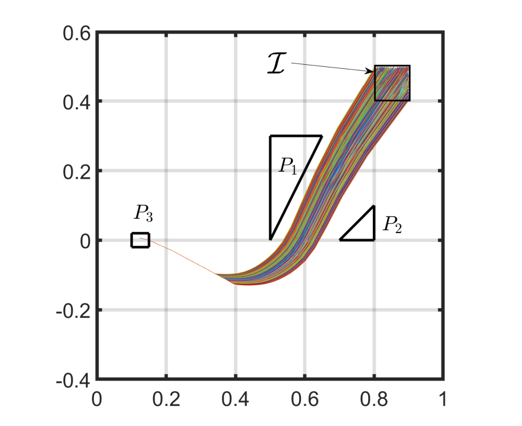
3D Nonlinear Feedback Control Model. Figure. 2 shows the trajectories of the nonlinear dynamical model shown in Eq. (8). The neural plant model is trained on $1.35\times 10^{6}$ transitions after discretizing the model with a sample time of $0.1$ seconds.

\begin{bmatrix}\dot{x}_{1}\\ \dot{x}_{2}\\ \dot{x}_{3}\end{bmatrix}=\begin{bmatrix}x_{1}^{3}+x_{2}\\ x_{2}^{3}+x_{3}\\ u\end{bmatrix},\ \mathcal{I}_{2}=\left\{\mathbf{s}_{0}\ \mid\ \begin{bmatrix}0.35\\ -0.35\\ 0.35\end{bmatrix}\leq\mathbf{s}_{0}\leq\begin{bmatrix}0.4\\ -0.3\\ 0.4\end{bmatrix}\right\}

(8)

We want to verify if the controller satisfies the formula $\varphi_{2}$ :

\varphi_{2}=\mathbf{F}_{[35,50]}\left[s\in P_{3}\right]\bigwedge\mathbf{G}_{[0,50]}\left[s\not\in P_{2}\right]\bigwedge\mathbf{G}_{[0,50]}\left[s\not\in P_{1}\right]

(9)

Adaptive Cruise Control. The third model we consider is a $\mathbf{ReLU}$ -NN plant model fit to a discretization of the $6$ -dimensional adaptive cruise control model described in Eq. (10) (sample time was $0.1s$ ). We used $1.5\times 10^{6}$ samples to train the plant model. In (10), the constant $\mu$ denotes a coefficient of friction set to $10^{-4}$ .

\begin{bmatrix}\dot{x}_{1}\\ \dot{x}_{2}\\ \dot{x}_{3}\\ \dot{x}_{4}\\ \dot{x}_{5}\\ \dot{x}_{6}\end{bmatrix}=\begin{bmatrix}x_{2}\\ x_{3}\\ -2x_{3}-4-\mu x_{2}^{2}\\ x_{5}\\ x_{6}\\ -2x_{6}+2u-\mu x_{4}^{2}\end{bmatrix},\ \mathcal{I}_{3}=\left\{\mathbf{s}_{0}\ \middle|\ \begin{bmatrix}90\\ 32\\ 0\\ 10\\ 30\\ 0\end{bmatrix}\leq\mathbf{s}_{0}\leq\begin{bmatrix}110\\ 32.2\\ 0\\ 11\\ 30.2\\ 0\end{bmatrix}\right\}

(10)

The NN-controller receives the observation, $O=[V_{set},\ t_{gap},\ x_{5}(k),x_{1}(k)-x_{4}(k),\ x_{2}(k)-x_{5}(k)]$ and returns the optimal control to satisfy the proposed STL specification (11) within $50$ time steps. Here $V_{set}=30$ , and $t_{gap}=1.4$ are fixed.

$\varphi_{3}=\mathbf{G}_{[0,50]}\left(\left[x_{1}(k)-x_{4}(k)<d_{safe}\right]\implies\mathbf{F}_{[0,3]}\left[x_{1}(k)-x_{4}(k)>d_{safe}^{*}\right]\right)$

(11)

where , $d_{safe}^{*}=12+1.4x_{5}(k)$ and $d_{safe}=10+1.4x_{5}(k)$ .

If the friction coefficient $\mu=0$ , then the model becomes an LTI system, and we can perform STL verification of the NNCS (where the plant has LTI dynamics).

Model to test Scalability with respect to Complexity of STL Formula.

To evaluate the scalability of our method with the complexity of the STL specification, we constructed a simple $2D$ plant model and a controller that takes $2$ inputs and produces $2$ outputs (both are $\mathbf{ReLU}$ -NNs). The actual model does not have any physical meaning (we show the model trajectories in Appendix 0.A for reference). The initial set of states $\mathcal{I}_{4}$ is $\left\{\mathbf{s}_{0}\ |\ \begin{bmatrix}1&1\end{bmatrix}^{\top}\leq\mathbf{s}_{0}\leq\begin{bmatrix}2&2\end{bmatrix}^{\top}\right\}$ . We gradually increase the complexity of the STL spec to analyze the runtime for verification using the exact-star reachability technique. The STL formulas we use as verification targets are shown in (12)-(14). We want to show that the formula in (15) is not satisfied by all initial states. The difference in formula $\varphi_{6}$ and $\varphi_{7}$ is in the time interval colored in red in $\varphi_{7}$ .

$\displaystyle\varphi_{4}$	$\displaystyle=$	$\displaystyle\mathbf{F}_{[5,8]}\left(s\in P_{1}\wedge\mathbf{F}_{[20,24]}s\in P_{4}\right)$	(12)
$\displaystyle\varphi_{5}$	$\displaystyle=$	$\displaystyle\mathbf{F}_{[5,8]}\left(s\in P_{1}\wedge\mathbf{F}_{[6,11]}\left(s\in P_{2}\wedge\mathbf{F}_{[12,16]}s\in P_{4}\right)\right)$	(13)
$\displaystyle\varphi_{6}$	$\displaystyle=$	$\displaystyle\mathbf{F}_{[5,8]}\left(s\in P_{1}\wedge\mathbf{F}_{[6,11]}\left(s\in P_{2}\wedge\mathbf{F}_{[6,7]}\left(s\in P_{3}\wedge\mathbf{F}_{[8,9]}s\in P_{4}\right)\right)\right)$	(14)
$\displaystyle\varphi_{7}$	$\displaystyle=$	$\displaystyle\mathbf{F}_{[5,8]}\left(s\in P_{1}\wedge\mathbf{F}_{[6,11]}\left(s\in P_{2}\wedge\mathbf{F}_{[6,7]}\left(s\in P_{3}\wedge\mathbf{F}_{{\color[rgb]{1,0,0}[9,10]}}s\in P_{4}\right)\right)\right)$	(15)

Practical Exponential Stability. We next consider a linear plant model (Eq. (16)) and a $\mathbf{ReLU}$ -NN controller that tries to stabilize the system to satisfy a practical exponential stability criterion as expressed by the STL formula $\varphi_{8}$ in (17); note that in $\varphi_{8}$ , $P_{6}\subset P_{5}\subset\cdots\subset P_{2}\subset P_{1}$ .

\mathbf{s}_{k+1}=A\mathbf{s}_{k}+Bu(\mathbf{s}_{k}),\ A=\begin{bmatrix}0.9105&-0.9718\\ 0.5177&0.3552\end{bmatrix},\ B=\begin{bmatrix}0.21&0.05\\ 0.15&-0.28\end{bmatrix}.

(16)

\begin{array}[]{ll}\varphi_{8}=&\mathbf{G}_{[9,16]}\left[s\in P_{1}\right]\wedge\mathbf{G}_{[17,24]}\left[s\in P_{2}\right]\wedge\mathbf{G}_{[25,32]}\left[s\in P_{3}\right]\wedge\\ &\mathbf{G}_{[33,40]}\left[s\in P_{4}\right]\wedge\mathbf{G}_{[41,43]}\left[s\in P_{5}\right]\wedge\mathbf{G}_{[44,60]}\left[s\in P_{6}\right]\end{array}

(17)

The architecture of NN controller is $\left[2,\ 30,\ 30,\ 30,\ 2\right]$ . We attempt to verify if the controller satisfies the mentioned STL specification for the inital state set $\mathcal{I}=\left\{(x,y)|x\in[-50,-40],\ y\in[85,95]\right\}$ . The regions $P_{5}$ and $P_{6}$ are small. This requires us to apply exact-star technique. On the other hand the exact-star is time consuming on $\mathcal{I}$ but partitioning $\mathcal{I}$ in $25$ partitions is quite helpful to verify within a reasonable running time. The results are presented in Table 2.

$\mathcal{I}$	Robustness Range	Run-time	Verified?	$\mathcal{I}$	Robustness Range	Run-time	Verified?
$x\in[-50,-48],y\in[85,87]$	$\left[0.2380,\ 0.3173\right]$	3199.4 $\mathrm{sec}$	Yes	$x\in[-50,-48],y\in[87,89]$	$\left[0.2414,\ 0.2884\right]$	28.22 $\mathrm{sec}$	Yes
$x\in[-50,-48],y\in[89,91]$	$\left[0.2383,\ 0.2638\right]$	13.19 $\mathrm{sec}$	Yes	$x\in[-50,-48],y\in[91,93]$	$\left[0.2151,\ 0.2429\right]$	114.3 $\mathrm{sec}$	Yes
$x\in[-50,-48],y\in[93,95]$	$\left[0.1927,\ 0.2244\right]$	199.8 $\mathrm{sec}$	Yes	$x\in[-48,-46],y\in[85,87]$	$\left[0.2539,\ 0.3130\right]$	287.3 $\mathrm{sec}$	Yes
$x\in[-48,-46],y\in[87,89]$	$\left[0.2435,\ 0.2881\right]$	2708.5 $\mathrm{sec}$	Yes	$x\in[-48,-46],y\in[89,91]$	$\left[0.2376,\ 0.2669\right]$	2645.6 $\mathrm{sec}$	Yes
$x\in[-48,-46],y\in[91,93]$	$\left[0.2183,\ 0.2468\right]$	45.8 $\mathrm{sec}$	Yes	$x\in[-48,-46],y\in[93,95]$	$\left[0.1934,\ 0.2228\right]$	6.8 $\mathrm{sec}$	Yes
$x\in[-46,-44],y\in[85,87]$	$\left[0.2824,\ 0.3140\right]$	467.9 $\mathrm{sec}$	Yes	$x\in[-46,-44],y\in[87,89]$	$\left[0.2550,\ 0.2916\right]$	1230.9 $\mathrm{sec}$	Yes
$x\in[-46,-44],y\in[89,91]$	$\left[0.2386,\ 0.2680\right]$	1408.4 $\mathrm{sec}$	Yes	$x\in[-46,-44],y\in[91,93]$	$\left[0.2138,\ 0.2432\right]$	610.1 $\mathrm{sec}$	Yes
$x\in[-46,-44],y\in[93,95]$	$\left[0.1889,\ 0.2183\right]$	16.7 $\mathrm{sec}$	Yes	$x\in[-44,-42],y\in[85,87]$	$\left[0.2839,\ 0.3133\right]$	7.9 $\mathrm{sec}$	Yes
$x\in[-44,-42],y\in[87,89]$	$\left[0.2590,\ 0.2884\right]$	36.4 $\mathrm{sec}$	Yes	$x\in[-44,-42],y\in[89,91]$	$\left[0.2341,\ 0.2635\right]$	152.2 $\mathrm{sec}$	Yes
$x\in[-44,-42],y\in[91,93]$	$\left[0.2092,\ 0.2386\right]$	796.4 $\mathrm{sec}$	Yes	$x\in[-44,-42],y\in[93,95]$	$\left[0.1844,\ 0.2138\right]$	1282.8 $\mathrm{sec}$	Yes
$x\in[-42,-40],y\in[85,87]$	$\left[0.2793,\ 0.3087\right]$	7.6 $\mathrm{sec}$	Yes	$x\in[-42,-40],y\in[87,89]$	$\left[0.2545,\ 0.2839\right]$	5.8 $\mathrm{sec}$	Yes
$x\in[-42,-40],y\in[89,91]$	$\left[0.2296,\ 0.2590\right]$	$6\mathrm{sec}$	Yes	$x\in[-42,-40],y\in[91,93]$	$\left[0.2047,\ 0.2341\right]$	$45.8\mathrm{sec}$	Yes
$x\in[-42,-40],y\in[93,95]$	$\left[0.1798,\ 0.2092\right]$	$142.4\mathrm{sec}$	Yes	—	—	—	—

Table 2: Verifying

\varphi_{8}

against NNCS in Eq. (16) utilizing exact-star reachability on TNN. Initial state set

\mathcal{I}=\left\{(x,y)|x\in[-50,-40],\ y\in[85,95]\right\}

. The trajectory encoding has

180

layers and

\mathsf{STL2NN}

has

8

layers. No parallel computing is utilized.

5 STL Verification using Sampling

Consider the TNN structure described in Sec. 4. If we compute the local Lipschitz constant of the function $\mathcal{R}_{\varphi}$ w.r.t. the initial state $\mathbf{s}_{0}$ , then we can use this to obtain a certificate that all initial states satisfy the given STL formula. The basic idea is that if we sample the set of initial states dense enough, and the value of $\mathcal{R}_{\varphi}$ is positive enough at all sample points, then this lets us reach a sound conclusion that $\mathcal{R}_{\varphi}$ is positive for all initial states. This intuition is formalized in Theorem 5.1.

Theorem 5.1

Assume $L_{loc}$ is the local Lipstchiz constant of function $f:\mathbb{R}^{n}\to\mathbb{R}$ on the domain $[\ell,u]$ where $\ell,u\in\mathbb{R}^{n}$ . We denote the set of all $2^{n}$ vertices on $[\ell,u]$ by $V([\ell,u])$ and we assume,

\forall x\in V([\ell,u])\ :\ f(x)>0

Given the certificates $\rho_{1}>L_{loc}$ and $\rho_{2}=\underset{x\in V([\ell,u])}{\min}f(x)$ ,

\|u-\ell\|_{2}<\frac{\rho_{2}}{\rho_{1}}\ \implies\forall x\in[\ell,u]\ :\ f(x)>0

Proof

Consider $x\in[\ell,u]$ and $x^{*}\in V([\ell,u]),\ f(x^{*})=\rho_{2}$ , this implies, $\|x^{*}-x\|_{2}\leq\|u-\ell\|_{2}$ . We know $\rho_{1}$ is an upper bound for the local Lipschitz constant $L_{loc}$ , therefore,

$\|\rho_{2}-f(x)\|_{2}\leq\rho_{1}\|x^{*}-x\|_{2}\leq\rho_{1}\|u-\ell\|_{2}\implies\|u-\ell\|_{2}\geq\frac{\|\rho_{2}-f(x)\|_{2}}{\rho_{1}}$

We will prove by contradiction that $f(x)>0$ . Assume $f(x)\leq 0$ . Since $\rho_{2}>0$ , we can conclude $\|u-\ell\|_{2}\geq\rho_{2}/\rho_{1}$ which contradicts our assumption. $\square$

The certificate $\rho_{1}$ , is an upper bound for the local Lipschitz constant of $\mathcal{R}_{\varphi}(\mathbf{s}_{0})$ with respect to the initial state, $\mathbf{s}_{0}\in\mathcal{I}$ . If a bounded certificate $\rho_{1}$ is accessible then we can utilize Theorem 5.1 for a sound and complete verification of controllers. Based on Theorem 5.1 we are required to select an $\epsilon>0$ to build an $\epsilon\!$ -net over the set of initial states. For every single hypercube in the $\epsilon$ -net we compute $\rho_{2}$ and check whether $\epsilon<\rho_{2}/\rho_{1}$ . In case this condition doesn’t hold we create a finer grid on the mentioned hypercube. We terminate the process, return the counter example and reject the controller if we face $\rho_{2}<0$ . Otherwise, we continue until $\epsilon<\rho_{2}/\rho_{1}$ for every single hypercube and verify the controller.

The efficiency of this technique is highly related to the tightness of the upper-bound $\rho_{1}$ . For instance, if the upper bound is large, to obtain a verification result, $\epsilon$ tends to be very small, greatly increasing the points over which to check the required condition. Thus, the key problem here is to solve the local Lipschitz constant computation for neural networks. This problem has been addressed by a variety of techniques in the literature [35], [5], [28], [24] but there is limitation on their time and memory scalability. The existent techniques in the literature are mostly limited to $\mathbf{ReLU}$ activation functions. There is also a trade-off between their scalability and accuracy.

In this paper, we use the convex programming technique presented in [15], [18] as convex programming scales to larger neural networks with low conservatism. The proposed technique [15], [18] in its current formulation is not directly applicable to our verification process but we can apply it with small modifications; the details are discussed in Appendix 0.A.2. We call this specific formulation of proposed convex programming in [18], [15] as $\mathsf{Trapezium\!\!-\!\!Lip\!\!-\!\!SDP}()$ . We remark that this method is applicable to plant and controller models that are neural networks with arbitrary activation functions or plants that have linear models. However, in its current form, we were not able to get conclusive verification results for arbitrary nonlinear ODE-based models (as local Lipschitz computation returned overly conservative Lipschitz constant values).

Function $\mathtt{Lip-Verify(}$ $\varphi,\rho_{1},\mathcal{I},\mathrm{model},\mathrm{controller},N,\mathsf{status}$ $\mathtt{)}$ 1

-

construct a uniform

\epsilon

-net of

N

hypercubes over

\mathcal{I}

\epsilon\text{-net}=\overset{N}{\underset{i=1}{\bigcup}}[\ell_{i},\ u_{i}]

\epsilon_{i}=\|u_{i}-\ell_{i}\|_{2}

while true do 2

for $i\leftarrow 1$ to $N$ do 3

if $\mathsf{status}\neq\mathsf{Solved}$ then 4

\rho_{1},\mathsf{status}\leftarrow\mathsf{Trapezium\!\!-\!\!Lip\!\!-\!\!SDP}([\ell_{i},\ u_{i}])

\rho_{2}\leftarrow\underset{x\in V([\ell_{i},\ u_{i}])}{\min}\mathcal{R}_{\varphi}(x)

if $\rho_{2}<0$ then 7

return Falsified + counter example
terminate; else 8

if $\left(\mathsf{status\neq\mathsf{Solved}}\right)\vee\left(\left(\mathsf{status}=\mathsf{Solved}\right)\wedge\left(\epsilon_{i}>\rho_{2}/\rho_{1}\right)\right)$ then 9

return

\mathtt{Lip-Verify(}

$\varphi,\rho_{1},[\ell_{i},\ u_{i}],\mathrm{model},\mathrm{controller},N,\mathsf{status}$

\mathtt{)}

return Verified

Algorithm 2 Recursive algorithm for verification with local Lipschitz certificates.

5.1 Experimental Validation

We now present results of applying our Lipschitz constant computation-based technique for verification.

Simple $\mathtt{tanh}$ -activation model. In this case study, we consider plant and controller models with structure $[4,\ 5,\ 2]$ , and $[2,\ 5,\ 2]$ respectively, where both models use the hyperbolic tangent activation function. In this problem we verify the STL formula shown in (18).Here, the specified set of initial states is provided as $\mathcal{I}=[1,2]\times[1,2]$ .

\varphi_{10}=\mathbf{F}_{[3,6]}\left(\ [s\in P_{1}]\ \wedge\ \mathbf{F}_{[9,13]}\ [s\in P_{2}]\right).

(18)

The TNN model contains a total of $38$ hidden tangent hyperbolic (+ linear) layers for encoding the trajectory and 10 hidden $\mathbf{ReLU}$ (+ linear) layers for $\mathsf{STL2NN}$ . We first partition $\mathcal{I}$ into 4 squares (see Figure 7) where $\epsilon=\sqrt{2}/2$ for each set. We employ the CROWN library [45] for the pre-activation bound computation on each trajectory layer. We also utilize the approx-star technique [42] for pre-activation bound computation on the $\mathsf{STL2NN}$ . Then we utilize convex programming approach $\mathsf{Trapezium\!\!-\!\!Lip\!\!-\!\!SDP}()$ ) that we developed with MOSEK [2] and YALMIP [31] solvers to compute $\rho_{1}$ . We also utilize $\mathsf{STL2NN}$ for each partition to compute the certificate $\rho_{2}$ . The results are shown in Figure 7. In the first round of partitioning, the desired condition $\epsilon\leq\rho_{2}/\rho_{1}$ does not hold for any partition. This implies we must partition all $4$ subsets (see Figure 7). In the next round of partitioning, $\epsilon=\sqrt{2}/4$ and $8$ subset from $16$ are verified satisfying $(\epsilon\leq\rho_{2}/\rho_{1})$ . For the remaining $8$ non-verified subsets we apply the third round of partitioning resulting in $\epsilon=\sqrt{2}/8$ where all of them become verified. Figure 2 presents the flow of recursive algorithm 2 With $3$ recursive calls. The verification concludes after 90 seconds with this algorithm.

Linear Time-Varying Plant. Figure 9 shows the evolution of control feedback system with the following LTV model, where,

A(\tau)=\begin{bmatrix}0&1\\ -2-sin(\tau)&-1\end{bmatrix},\ B=\begin{bmatrix}1\\ 0\end{bmatrix},\ T=\frac{2\pi}{30},\ \mathbf{s}_{k}=\begin{bmatrix}x_{k}\\ y_{k}\end{bmatrix}

which is the Zero-Order Hold discretization of $\dot{\mathbf{s}}=A(t)\mathbf{s}+B\eta(\mathbf{s})$ , with sampling time $T$ . The controller is a neural network of structure $[2,7,7,1]$ , with $\tanh()$ activation function and is expected to satisfy,

	$\displaystyle\varphi$	$\displaystyle=\mathbf{F}_{[30,35]}\left[x_{k}\leq-0.5\right]\bigwedge\mathbf{F}_{[37,43]}\left[x_{k}\geq-0.4\right]\bigwedge\mathbf{F}_{[45,50]}\left[x_{k}\leq 0\right]$
		$\displaystyle\bigwedge\mathbf{F}_{[32,38]}\left[y_{k}\geq 1\right]\bigwedge\mathbf{G}_{[1,50]}\left[y_{k}-x_{k}\leq 5.5\right].$

Since the parallel computing does not support recursive algorithms, we manually partition $\mathcal{I}:=\left\{\mathbf{s}_{0}\mid\begin{bmatrix}-1,-1\end{bmatrix}^{\top}\leq\mathbf{s}_{0}\leq\begin{bmatrix}0,0\end{bmatrix}^{\top}\right\}$ into 64 equal subsets, and run Algorithm 2 on every set. The average verification time for each sub-problem was around $6$ minutes. See Figure 13 for more detail.

Neural Network Controlled Quadrotor System. Figure 9 shows the evolution of control feedback system for a quadrotor. The model is trained on the following dynamics with $T=0.05$ and trajectories start from $\mathcal{I}$ ,

\begin{bmatrix}\dot{p}_{x}\\ \dot{p}_{y}\\ \dot{p}_{z}\\ \dot{v}_{x}\\ \dot{v}_{y}\\ \dot{v}_{z}\end{bmatrix}=\begin{bmatrix}v_{x}\\ v_{y}\\ v_{z}\\ \mathrm{g}\tan(\theta)\\ -\mathrm{g}\tan(\phi)\\ \tau-\mathrm{g}\end{bmatrix},\ \mathcal{I}=\left\{\mathbf{s}_{0}\ \mid\ \begin{bmatrix}0.0638\\ 0.0638\\ -0.0213\\ 0\\ 0\\ 0\end{bmatrix}\leq\mathbf{s}_{0}\leq\begin{bmatrix}0.1063\\ 0.1063\\ 0.0213\\ 0\\ 0\\ 0\end{bmatrix}\right\}

We train a $\tanh()$ FFNN on this dynamics using $3.696\times 10^{6}$ training data. The model ’s dimension is $[9,10,10,6]$ . The controller is also $\tanh()$ FFNN with dimension $[6,10,3,3]$ . We wish to verify the formula:

\varphi=\mathbf{F}_{[1,20]}\left(\left[s\in\mathcal{E}_{1}\right]\vee\left[s\in\mathcal{E}_{2}\right]\right)\bigwedge\mathbf{G}_{[1,20]}\left[s\notin\mathcal{E}_{3}\right]

Here the controller is time-varying and its first bias vector linearly varies with time. ( $b_{1}(k)=\bar{b}_{1}+k\delta b_{1}$ ). Since the parallel computing does not support recursive algorithms, we manually partition $\mathcal{I}$ into $64$ equal cubes and run the algorithm 2 on every one of them. The approximate running time for the majority of them was $40$ minutes. But for some regions the verification was time consuming. See Figure 12 for more detail.

6 Related Work & Conclusions

Related work. Safety verification of NNCS is well studied in the literature. We can classify these works in two categories. One group addresses open loop control systems. The authors in [25] present a verification technique based on Satisfiability Modulo Theories (SMT). They extend simplex to handle $\mathbf{ReLU}$ activation functions and propose an efficient verification for $\mathbf{ReLU}$ networks called ReLUplex. They also propose in [26] another technique based on SMT called Marabou, which is not restricted on $\mathbf{ReLU}$ activation function. The authors in [34] propose verification for multi-layer perceptrons using abstraction to Boolean combination of linear arithmetic constraints which is also based on SMT. The authors in [12], [27], [32] present several verification techniques that are based on Mixed Integer Linear Programming MILP and the works [3], [16], [38], [39], [46], [45], [47] are also considered as set based verification techniques. The other group addresses the closed loop NNCS. The authors in [40] propose sound and complete verification for discrete plants based on Satisfiability Modulo Convex (SMC) techniques. The authors in [11] propose a fast and efficient algorithm that is restricted on $\mathbf{ReLU}$ activation function based on regressive polynomial rule inference. For Verification on NNCS with ODE models the authors in [21] propose a reachability analysis on nonlinear plants employing Taylor series and Bernstein Polynomials. This method is not restricted on $\mathbf{ReLU}$ and is adjustable to control the level of conservatism. Falsification and test-based approaches are also introduced to the verification community with authors in [9, 10, 44].

Conclusion. We present $\mathsf{STL2NN}$ a $\mathbf{ReLU}$ network which can be utilized for neural network verification with general STL specifications over discrete time signals. Since the formulation of verification problem is highly dependent to the STL specifications we present Trapezium-FFNN as a basic structure for problem formulation which is quite helpful to provide a toolbox on this approach. This is the first toolbox for sound and complete verification with general STL specifications. Unlike the other verification toolboxes, this toolbox is not restricted to $\mathbf{ReLU}$ networks. For a neural network controlled system with difference equation models, our $\mathsf{STL2NN}$ can be applied on existing approximate reachability techniques such as ReachNN [21] to provide a sound but not complete verification.

Acknowledgement

The authors would like to thank the anonymous reviewers for their feedback. This work was supported by the National Science Foundation through the following grants: CAREER award $\mathsf{SHF-2048094}$ , $\mathsf{CNS-1932620}$ , and funding by Toyota R&D through the USC Center for Autonomy and AI.

References

[1] Akazaki, T., Hasuo, I.: Time robustness in mtl and expressivity in hybrid system falsification. In: International Conference on Computer Aided Verification. pp. 356–374. Springer (2015)
[2] Andersen, E.D., Andersen, K.D.: The mosek interior point optimizer for linear programming: an implementation of the homogeneous algorithm. In: High performance optimization, pp. 197–232. Springer (2000)
[3] Anderson, G., Pailoor, S., Dillig, I., Chaudhuri, S.: Optimization and abstraction: a synergistic approach for analyzing neural network robustness. In: Proceedings of the 40th ACM SIGPLAN Conference on Programming Language Design and Implementation. pp. 731–744 (2019)
[4] Atkinson, K., Han, W., Stewart, D.E.: Numerical solution of ordinary differential equations. John Wiley & Sons (2011)
[5] Avant, T., Morgansen, K.A.: Analytical bounds on the local lipschitz constants of affine-relu functions. arXiv preprint arXiv:2008.06141 (2020)
[6] Chua, K., Calandra, R., McAllister, R., Levine, S.: Deep reinforcement learning in a handful of trials using probabilistic dynamics models. Advances in neural information processing systems 31 (2018)
[7] Deisenroth, M.P., Fox, D., Rasmussen, C.E.: Gaussian processes for data-efficient learning in robotics and control. IEEE transactions on pattern analysis and machine intelligence 37(2), 408–423 (2013)
[8] Donzé, A., Maler, O.: Robust satisfaction of temporal logic over real-valued signals. In: International Conference on Formal Modeling and Analysis of Timed Systems. pp. 92–106. Springer (2010)
[9] Dreossi, T., Donzé, A., Seshia, S.A.: Compositional falsification of cyber-physical systems with machine learning components. Journal of Automated Reasoning 63(4), 1031–1053 (2019)
[10] Dreossi, T., Fremont, D.J., Ghosh, S., Kim, E., Ravanbakhsh, H., Vazquez-Chanlatte, M., Seshia, S.A.: Verifai: A toolkit for the formal design and analysis of artificial intelligence-based systems. In: International Conference on Computer Aided Verification. pp. 432–442. Springer (2019)
[11] Dutta, S., Chen, X., Sankaranarayanan, S.: Reachability analysis for neural feedback systems using regressive polynomial rule inference. In: Proceedings of the 22nd ACM International Conference on Hybrid Systems: Computation and Control. pp. 157–168 (2019)
[12] Dutta, S., Jha, S., Sanakaranarayanan, S., Tiwari, A.: Output range analysis for deep neural networks. arXiv preprint arXiv:1709.09130 (2017)
[13] Ehlers, R.: Formal verification of piece-wise linear feed-forward neural networks. In: International Symposium on Automated Technology for Verification and Analysis. pp. 269–286. Springer (2017)
[14] Fainekos, G.E., Pappas, G.J.: Robustness of temporal logic specifications. In: Formal approaches to software testing and runtime verification, pp. 178–192. Springer (2006)
[15] Fazlyab, M., Robey, A., Hassani, H., Morari, M., Pappas, G.: Efficient and accurate estimation of lipschitz constants for deep neural networks. Advances in Neural Information Processing Systems 32 (2019)
[16] Gehr, T., Mirman, M., Drachsler-Cohen, D., Tsankov, P., Chaudhuri, S., Vechev, M.: Ai2: Safety and robustness certification of neural networks with abstract interpretation. In: 2018 IEEE symposium on security and privacy (SP). pp. 3–18. IEEE (2018)
[17] Goodfellow, I., Bengio, Y., Courville, A.: Deep learning. MIT press (2016)
[18] Hashemi, N., Ruths, J., Fazlyab, M.: Certifying incremental quadratic constraints for neural networks via convex optimization. In: Learning for Dynamics and Control. pp. 842–853. PMLR (2021)
[19] Ho, H.M., Ouaknine, J., Worrell, J.: Online monitoring of metric temporal logic. In: International Conference on Runtime Verification. pp. 178–192. Springer (2014)
[20] Huang, C., Fan, J., Chen, X., Li, W., Zhu, Q.: Polar: A polynomial arithmetic framework for verifying neural-network controlled systems. arXiv preprint arXiv:2106.13867 (2021)
[21] Huang, C., Fan, J., Li, W., Chen, X., Zhu, Q.: Reachnn: Reachability analysis of neural-network controlled systems. ACM Transactions on Embedded Computing Systems (TECS) 18(5s), 1–22 (2019)
[22] Huang, X., Kwiatkowska, M., Wang, S., Wu, M.: Safety verification of deep neural networks. In: International conference on computer aided verification. pp. 3–29. Springer (2017)
[23] Ivanov, R., Weimer, J., Alur, R., Pappas, G.J., Lee, I.: Verisig: verifying safety properties of hybrid systems with neural network controllers. In: Proceedings of the 22nd ACM International Conference on Hybrid Systems: Computation and Control. pp. 169–178 (2019)
[24] Jordan, M., Dimakis, A.G.: Exactly computing the local lipschitz constant of relu networks. Advances in Neural Information Processing Systems 33, 7344–7353 (2020)
[25] Katz, G., Barrett, C., Dill, D.L., Julian, K., Kochenderfer, M.J.: Reluplex: An efficient smt solver for verifying deep neural networks. In: International conference on computer aided verification. pp. 97–117. Springer (2017)
[26] Katz, G., Huang, D.A., Ibeling, D., Julian, K., Lazarus, C., Lim, R., Shah, P., Thakoor, S., Wu, H., Zeljić, A., et al.: The marabou framework for verification and analysis of deep neural networks. In: International Conference on Computer Aided Verification. pp. 443–452. Springer (2019)
[27] Kouvaros, P., Lomuscio, A.: Formal verification of cnn-based perception systems. arXiv preprint arXiv:1811.11373 (2018)
[28] Latorre, F., Rolland, P., Cevher, V.: Lipschitz constant estimation of neural networks via sparse polynomial optimization. arXiv preprint arXiv:2004.08688 (2020)
[29] Li, J., Liu, J., Yang, P., Chen, L., Huang, X., Zhang, L.: Analyzing deep neural networks with symbolic propagation: Towards higher precision and faster verification. In: International static analysis symposium. pp. 296–319. Springer (2019)
[30] Liu, C., Arnon, T., Lazarus, C., Strong, C., Barrett, C., Kochenderfer, M.J., et al.: Algorithms for verifying deep neural networks. Foundations and Trends® in Optimization 4(3-4), 244–404 (2021)
[31] Lofberg, J.: Yalmip: A toolbox for modeling and optimization in matlab. In: 2004 IEEE international conference on robotics and automation (IEEE Cat. No. 04CH37508). pp. 284–289. IEEE (2004)
[32] Lomuscio, A., Maganti, L.: An approach to reachability analysis for feed-forward relu neural networks. arXiv preprint arXiv:1706.07351 (2017)
[33] Maler, O., Nickovic, D.: Monitoring temporal properties of continuous signals. In: Formal Techniques, Modelling and Analysis of Timed and Fault-Tolerant Systems, pp. 152–166. Springer (2004)
[34] Pulina, L., Tacchella, A.: An abstraction-refinement approach to verification of artificial neural networks. In: International Conference on Computer Aided Verification. pp. 243–257. Springer (2010)
[35] Raghunathan, A., Steinhardt, J., Liang, P.S.: Semidefinite relaxations for certifying robustness to adversarial examples. Advances in Neural Information Processing Systems 31 (2018)
[36] Rasmussen, C.E.: Gaussian processes in machine learning. In: Summer school on machine learning. pp. 63–71. Springer (2003)
[37] Rodionova, A., Lindemann, L., Morari, M., Pappas, G.J.: Combined left and right temporal robustness for control under stl specifications. IEEE Control Systems Letters (2022)
[38] Singh, G., Gehr, T., Mirman, M., Püschel, M., Vechev, M.: Fast and effective robustness certification. Advances in neural information processing systems 31 (2018)
[39] Singh, G., Gehr, T., Püschel, M., Vechev, M.: An abstract domain for certifying neural networks. Proceedings of the ACM on Programming Languages 3(POPL), 1–30 (2019)
[40] Sun, X., Khedr, H., Shoukry, Y.: Formal verification of neural network controlled autonomous systems. In: Proceedings of the 22nd ACM International Conference on Hybrid Systems: Computation and Control. pp. 147–156 (2019)
[41] Szegedy, C., Zaremba, W., Sutskever, I., Bruna, J., Erhan, D., Goodfellow, I., Fergus, R.: Intriguing properties of neural networks. arXiv preprint arXiv:1312.6199 (2013)
[42] Tran, H.D., Manzanas Lopez, D., Musau, P., Yang, X., Nguyen, L.V., Xiang, W., Johnson, T.T.: Star-based reachability analysis of deep neural networks. In: International symposium on formal methods. pp. 670–686. Springer (2019)
[43] Tran, H.D., Yang, X., Manzanas Lopez, D., Musau, P., Nguyen, L.V., Xiang, W., Bak, S., Johnson, T.T.: Nnv: the neural network verification tool for deep neural networks and learning-enabled cyber-physical systems. In: International Conference on Computer Aided Verification. pp. 3–17. Springer (2020)
[44] Tuncali, C.E., Fainekos, G., Ito, H., Kapinski, J.: Simulation-based adversarial test generation for autonomous vehicles with machine learning components. In: 2018 IEEE Intelligent Vehicles Symposium (IV). pp. 1555–1562. IEEE (2018)
[45] Wang, S., Pei, K., Whitehouse, J., Yang, J., Jana, S.: Efficient formal safety analysis of neural networks. Advances in Neural Information Processing Systems 31 (2018)
[46] Wang, S., Pei, K., Whitehouse, J., Yang, J., Jana, S.: Formal security analysis of neural networks using symbolic intervals. In: 27th USENIX Security Symposium (USENIX Security 18). pp. 1599–1614 (2018)
[47] Xiang, W., Tran, H.D., Johnson, T.T.: Output reachable set estimation and verification for multilayer neural networks. IEEE transactions on neural networks and learning systems 29(11), 5777–5783 (2018)
[48] Zhang, H., Weng, T.W., Chen, P.Y., Hsieh, C.J., Daniel, L.: Efficient neural network robustness certification with general activation functions. Advances in neural information processing systems 31 (2018)

Appendix 0.A Appendix

0.A.1 Logarithmic Extension for Lemma 1

We are interested in an extension for Lemma 1 that provides a network with depth of logarithmic order corresponding to the number of inputs. Thus we group the inputs in pairs of two and apply Lemma 1 repeatedly. Figure 10 clarifies this extension for a set of $7$ inputs.

0.A.2 Lipschitz Constant Analysis for TNN

Upper bound for local Lipschitz constant of a FFNN is derived in [18], [15]. The presence of linear activation functions in $\mathsf{STL2NN}$ must not impose computational complexity but if we include them in the proposed procedure in [18], [15] the optimization process faces memory problems as the size of LMI increases unnecessarily. Thus we slightly modify the proposed solution. We call this slightly modified version as $\mathsf{Trapezium\!\!-\!\!Lip\!\!-\!\!SDP}()$ . Here we propose a summary of the convex programming approach from [18], [15] including the slight changes we apply on it.

Let’s define the SDP variable $\rho=\rho_{1}^{2}$ . We can reformulate the Lipschitz inequality $\|f(x_{1})-f(x_{2})\|_{2}\leq\sqrt{\rho}\|x_{1}-x_{2}\|_{2}$ in the form of linear quadratic constraint as follows:

\begin{bmatrix}x_{1}-x_{2}\\ f(x_{1})-f(x_{2})\end{bmatrix}^{\top}\begin{bmatrix}\rho I_{n}&0_{n\times 1}\\ 0_{1\times n}&-1\end{bmatrix}\begin{bmatrix}x_{1}-x_{2}\\ f(x_{1})-f(x_{2})\end{bmatrix}\geq 0

and we can conclude if,

\begin{bmatrix}\rho I_{n}&0_{n\times 1}\\ 0_{1\times n}&-1\end{bmatrix}\geq 0\ \text{(positive semi-definite)}

then $\rho_{1}=\sqrt{\rho}$ is certainly the desired certificate. Unfortunately due to presence of the negative scalar $-1$ , this constraint is infeasible and we attempt to provide feasibility with provision of new linear information about function $f$ . Thus the basic idea of convex programming technique is to provide the best symmetric linear matrix $Q_{\mathrm{info}}$ and transformation matrix $T$ that bring feasibility for,

Q_{\mathrm{info}}-T^{\top}\begin{bmatrix}\rho I_{n}&0_{n\times 1}\\ 0_{1\times n}&-1\end{bmatrix}T\leq 0,

(19)

where $Q_{\mathrm{info}}$ is a linear combination of quadratic constraints (QC), where every single QC represents a linear information about function $f$ . In this constraint $\rho=\rho_{1}^{2}$ , where $\rho_{1}$ is the certificate introduced in Theorem 5.1 for $f:[\ell,\ u]\to[a,\ b]$ , $\ell,u\in\mathbb{R}^{n}$ and $a,b\in\mathbb{R}$ . We add new information utilizing s-procedure technique proposed in [15], [18]. A thorough introduction for computation of $Q_{\mathrm{info}}$ is provided in [15], [18]. Provision of high quality information results in feasibility and tightness, but the presence of insufficient information results in infeasibility.

QC for Non-linearities in feed-back structure:

Figure 11 shows the layers of TNN. The layers of TNN are entitled with $n=1,\cdots,N$ . These layers are departed into nonlinear and linear portions. The pre-activation of nonlinear portion, $p_{\ell}$ is fed in nonlinear portion and results in post-activation $z_{\ell}$ .

Assume $\mathbf{s}_{0}^{1},\mathbf{s}_{0}^{2}$ are two initial states. They provide the pre-activations $p_{\ell}^{1},p_{\ell}^{2}\in\mathbb{R}^{n_{\ell}}$ on the TNN. The post-activations are also $z_{\ell}^{1},z_{\ell}^{2}\in\mathbb{R}^{n_{\ell}}$ respectively. We denote $\delta p_{\ell}:=p_{\ell}^{1}-p_{\ell}^{2}$ , $\delta z_{\ell}:=z_{\ell}^{1}-z_{\ell}^{2}$ . We inform the convex programming about nonlinearities in $\mathcal{R}_{\varphi}(\mathbf{s}_{0})$ through the following quadratic constraints:
-

The nonlinearity is a vector of differentiable activation functions.

Lemma 3

[18]: Let $\phi(w)=(\sigma(w_{1}),\cdots,\sigma(w_{n})),\ w\in\mathcal{X}\subseteq\mathbb{R}^{m}$ , where $\sigma$ is differentiable. Define $e_{i}^{\top}\vec{\alpha}=\inf_{w\in\mathcal{X}}\ \sigma^{\prime}(w_{i})$ and $e_{i}^{\top}\vec{\beta}=\sup_{w\in\mathcal{X}}\ \sigma^{\prime}(w_{i})$ . Then $\phi$ satisfies the $\delta\mathrm{QC}$ defined by $(\mathcal{X},\mathcal{Q})$ , where

$\begin{aligned} \mathcal{Q}=\{Q\mid Q=\begin{bmatrix}-2\operatorname{diag}(\vec{\alpha}\circ\vec{\beta}\circ\lambda)&\operatorname{diag}((\vec{\alpha}+\vec{\beta})\circ\lambda)\\ \operatorname{diag}((\vec{\alpha}+\vec{\beta})\circ\lambda)&-2\operatorname{diag}(\lambda)\end{bmatrix},\ \lambda\in\mathbb{R}^{m}_{+}\}.\end{aligned}$

(20)

Thus, we firstly compute vector of slope bounds through the pre-activation bound computation and as an example given the slope bounds $\vec{\alpha}_{\ell}$ and $\vec{\beta}_{\ell}$ on the $\ell$ -th layer of TNN we claim:

$\begin{bmatrix}\delta p_{\ell}\\ \delta z_{\ell}\end{bmatrix}^{\top}\underbrace{\begin{bmatrix}-2\operatorname{diag}(\vec{\alpha}_{\ell}\circ\vec{\beta}_{\ell}\circ\lambda_{\ell})&\operatorname{diag}((\vec{\alpha}_{\ell}+\vec{\beta}_{\ell})\circ\lambda_{\ell})\\ \operatorname{diag}((\vec{\alpha}_{\ell}+\vec{\beta}_{\ell})\circ\lambda_{\ell})&-2\operatorname{diag}(\lambda_{\ell})\end{bmatrix}}_{Q_{\ell}}\begin{bmatrix}\delta p_{\ell}\\ \delta z_{\ell}\end{bmatrix}\geq 0,\ \lambda_{\ell}\in\mathbb{R}^{n_{\ell}}_{+}\\$

The nonlinearity is a vector of non-differentiable activation functions.

Lemma 4

[18]: Let $\phi(w)=\max(\alpha w,\beta w),\ w\in\mathcal{X}\subseteq\mathbb{R}^{m},0\leq\alpha\leq\beta<\infty$ and define $\mathcal{I}^{+}$ , $\mathcal{I}^{-}$ , and $\mathcal{I}^{\pm}$ as the set of activations that are known to be always active, always inactive, or unknown on $\mathcal{X}$ , i.e., $\mathcal{I}^{+}=\{i\mid w_{i}\geq 0,\forall w\in\mathcal{X}\}$ , $\mathcal{I}^{-}=\{i\mid w_{i}<0,\forall w\in\mathcal{X}\}$ , and $\mathcal{I}^{\pm}=\{1,\cdots,m\}\setminus(\mathcal{I}^{+}\cup\mathcal{I}^{-})$ . Define $\boldsymbol{\alpha}=[\alpha+(\beta-\alpha)\mathbf{1}_{\mathcal{I}^{+}}(1),\cdots,\alpha+(\beta-\alpha)\mathbf{1}_{\mathcal{I}^{+}}(m)]$ and $\boldsymbol{\beta}=[\beta-(\beta-\alpha)\mathbf{1}_{\mathcal{I}^{-}}(1),\cdots,\beta-(\beta-\alpha)\mathbf{1}_{\mathcal{I}^{-}}(m)]$ . Then $\phi$ satisfies the $\delta\mathrm{QC}$ defined by $(\mathcal{X},\mathcal{Q})$ , where

	$\displaystyle\mathcal{Q}=\{Q\mid Q$	$\displaystyle=\begin{bmatrix}-2\operatorname{diag}(\boldsymbol{\alpha}\circ\boldsymbol{\beta}\circ\lambda)&\operatorname{diag}((\boldsymbol{\alpha}+\boldsymbol{\beta})\circ\lambda)\\ \operatorname{diag}((\boldsymbol{\alpha}+\boldsymbol{\beta})\circ\lambda)&-2\operatorname{diag}(\lambda)\end{bmatrix},$		(21)
		$\displaystyle e_{i}^{\top}\lambda\in\mathbb{R}_{+}\ \text{ for }i\in\mathcal{I}^{\pm}\}.$		(21)

Therefore, To capture the slope bounds, we firstly determine $\mathcal{I}^{+},\mathcal{I}^{-}$ through the pre-activation bound computation and as an example given the slope bounds $\boldsymbol{\alpha}_{\ell}$ and $\boldsymbol{\beta}_{\ell}$ on the $\ell$ -th layer of TNN we claim for, $e_{j}^{\top}\lambda_{\ell}\in\mathbb{R}_{+}\ \text{ and }j\in\mathcal{I}^{\pm}$ :

\begin{bmatrix}\delta p_{\ell}\\ \delta z_{\ell}\end{bmatrix}^{\top}\underbrace{\begin{bmatrix}-2\operatorname{diag}(\boldsymbol{\alpha}_{\ell}\circ\boldsymbol{\beta}_{\ell}\circ\lambda_{\ell})&\operatorname{diag}((\boldsymbol{\alpha}_{\ell}+\boldsymbol{\beta}_{\ell})\circ\lambda_{\ell})\\ \operatorname{diag}((\boldsymbol{\alpha}_{\ell}+\boldsymbol{\beta}_{\ell})\circ\lambda_{\ell})&-2\operatorname{diag}(\lambda_{\ell})\end{bmatrix}}_{Q_{\ell}}\begin{bmatrix}\delta p_{\ell}\\ \delta z_{\ell}\end{bmatrix}\geq 0,

S-procedure for $Q_{\text{info}}$ :

Consider the weigh matrices on TNN in Figure 11. This weigh matrices are built from $4$ sub-blocks,

•

$W_{\ell}^{ll}$ : This subblock connects the linear portion of layer $\ell-1$ to linear portion of layer $\ell$ .
•

$W_{\ell}^{ln}$ : This subblock connects the linear portion of layer $\ell-1$ to non-linear portion of layer $\ell$ .
•

$W_{\ell}^{nl}$ : This subblock connects the non-linear portion of layer $\ell-1$ to linear portion of layer $\ell$ .
•

$W_{\ell}^{nn}$ : This subblock connects the non-linear portion of layer $\ell-1$ to non-linear portion of layer $\ell$ .

Therefore the pre-activation $p_{\ell}$ is computed as a linear combination of previous activations $z_{i},i=0,\cdots,\ell-1$ through the following iterative formula.

\begin{bmatrix}t_{1}\\ p_{1}\end{bmatrix}=\underbrace{\begin{bmatrix}W_{1}^{ln}\\ \\ \hline\cr\\ W_{1}^{nn}\end{bmatrix}}_{W_{1}}\underbrace{z_{0}}_{\mathbf{s}_{0}}+b_{1},\ \begin{bmatrix}t_{\ell}\\ \\ p_{\ell}\end{bmatrix}=\underbrace{\left[\begin{matrix}\begin{array}[]{c|c}W_{\ell}^{ll}&\hskip 5.69054ptW_{\ell}^{ln}\\ \\ \hline\cr\\ W_{\ell}^{nl}&\hskip 5.69054ptW_{\ell}^{nn}\end{array}\end{matrix}\right]}_{W_{\ell},\ \ \ell=2,\cdots,N}\begin{bmatrix}t_{\ell-1}\\ \\ {z_{\ell-1}}\end{bmatrix}+b_{\ell},\

then the difference of pre-activations $\delta p_{\ell}$ are,

$\begin{aligned} &\delta p_{1}=W_{1}^{nn}(\delta z_{0}),\quad\delta p_{2}=W_{2}^{nl}W_{1}^{ln}\delta z_{1}+W_{2}^{nn}\delta z_{0}\\ &\delta p_{\ell}=W_{\ell}^{nl}\sum_{k=0}^{\ell-3}\left[\left(\prod_{j=1}^{\ell-k-2}W_{\ell-j}^{ll}\right)W_{k+1}^{ln}(\delta z_{k})\right]+W_{\ell}^{nl}W_{\ell-1}^{ln}(\delta z_{\ell-2})+W_{\ell}^{nn}\delta z_{\ell-1},\ \ell\geq 3\end{aligned}$

We also follow the process of [18], [15] and concatenate the non-linear activation vectors in the base vector $\delta Z:=[\delta z_{0}^{\top},\cdots,\delta z_{N}^{\top}]^{\top}$ . Given the proposed relation between $\delta p_{\ell}$ and $\delta Z$ we define the transformation matrix $E_{\ell},T$ as,

\begin{bmatrix}\delta p_{\ell}\\ \delta z_{\ell}\end{bmatrix}=E_{\ell}\ \delta Z,\ \ell=1,\cdots,N,\ \begin{bmatrix}\delta z_{0}\\ W_{N+1}\delta z_{N}\end{bmatrix}=T\ \delta Z

Finally based on the idea in [18], [15], we claim if,

\sum_{\ell=1}^{N}\begin{bmatrix}\delta p_{\ell}\\ \delta z_{\ell}\end{bmatrix}^{\top}Q_{\ell}\begin{bmatrix}\delta p_{\ell}\\ \delta z_{\ell}\end{bmatrix}-\begin{bmatrix}\delta z_{0}\\ W_{N+1}\delta z_{N}\end{bmatrix}^{\top}\begin{bmatrix}\rho I_{n}&0_{n\times 1}\\ 0_{1\times n}&-1\end{bmatrix}\begin{bmatrix}\delta z_{0}\\ W_{N+1}\delta z_{N}\end{bmatrix}\leq 0

(22)

Then, $\left\|\mathcal{R}_{\varphi}(\mathbf{s}_{0}^{1})-\mathcal{R}_{\varphi}(\mathbf{s}_{0}^{2})\right\|_{2}\leq\sqrt{\rho}\left\|\mathbf{s}_{0}^{1}-\mathbf{s}_{0}^{2}\right\|_{2}$ and this is because equation (22) implies,

\begin{bmatrix}\delta z_{0}\\ W_{N+1}\delta z_{N}\end{bmatrix}^{\top}\begin{bmatrix}\rho I_{n}&0_{n\times 1}\\ 0_{1\times n}&-1\end{bmatrix}\begin{bmatrix}\delta z_{0}\\ W_{N+1}\delta z_{N}\end{bmatrix}\geq 0

This result certifies $\rho_{1}=\sqrt{\rho}$ to be a true certificate as an upper bound of Lipschitz constant. On the other hand equation (22) can be rephrased based on the base vector $\delta Z$ as,

\delta Z^{\top}\left(\sum_{\ell=1}^{N}E_{\ell}^{\top}Q_{\ell}E_{\ell}-T^{\top}\begin{bmatrix}\rho I_{n}&0_{n\times 1}\\ 0_{1\times n}&-1\end{bmatrix}T\right)\delta Z\leq 0

(23)

and proposing $Q_{\text{info}}=\sum_{\ell=1}^{N}E_{\ell}^{\top}Q_{\ell}E_{\ell}$ a sufficient condition to satisfy (23) is,

Q_{\text{info}}-T^{\top}\begin{bmatrix}\rho I_{n}&0_{n\times 1}\\ 0_{1\times n}&-1\end{bmatrix}T\leq 0

A Neurosymbolic Approach to the Verification of Temporal Logic Properties of Learning enabled Control Systems

Abstract

Keywords:

1 Introduction

2 Preliminaries

3 STL Robustness as a Neural Network

Lemma 1

Proof

Lemma 2

Theorem 3.1

4 STL Verification using Reachability

4.1 Trapezium feed-forward Neural Network (TNN)

4.2 STL verification using reachability analysis

Assumption 1

Theorem 4.1

Proof

Remark 1

4.3 Experimental Evaluation: STL verification with NN reachability

5 STL Verification using Sampling

Theorem 5.1

Proof

5.1 Experimental Validation

6 Related Work & Conclusions

Acknowledgement

References

Appendix 0.A Appendix

0.A.1 Logarithmic Extension for Lemma 1

0.A.2 Lipschitz Constant Analysis for TNN

QC for Non-linearities in feed-back structure:

Lemma 3

Lemma 4

S-procedure for QinfoQ_{\text{info}}:

S-procedure for $Q_{\text{info}}$ :