跳到论文正文
W Papers独立论文阅读器 arXiv:2303.05365 论文正文 计算阅读时间 · 0%
引用这篇论文根据当前论文元数据生成,正式投稿前建议核对。


License: CC BY 4.0
arXiv:2303.05365v1 [math.NA] 09 Mar 2023

Spherical framelets from spherical designsThanks: Submitted to editors DATE.

Yuchen Xiao Email: yc.xiao@my.cityu.edu.hk Thanks: Department of Mathematics, City University of Hong Kong, Tat Chee Avenue, Kowloon Tong, Hong Kong ().    Xiaosheng Zhuang Email: xzhuang7@cityu.edu.hk Thanks: Department of Mathematics, City University of Hong Kong, Tat Chee Avenue, Kowloon Tong, Hong Kong ().
Abstract

In this paper, we investigate in detail the structures of the variational characterization AN,tA_{N,t} of the spherical tt-design, its gradient ∇AN,t\nabla A_{N,t}, and its Hessian ℋ⁡(AN,t)\mathcal{H}(A_{N,t}) in terms of fast spherical harmonic transforms. Moreover, we propose solving the minimization problem of AN,tA_{N,t} using the trust-region method to provide spherical tt-designs with large values of tt. Based on the obtained spherical tt-designs, we develop (semi-discrete) spherical tight framelets as well as their truncated systems and their fast spherical framelet transforms for the practical spherical signal/image processing. Thanks to the large spherical tt-designs and localization property of our spherical framelets, we are able to provide signal/image denoising using local thresholding techniques based on a fine-tuned spherical cap restriction. Many numerical experiments are conducted to demonstrate the efficiency and effectiveness of our spherical framelets, including Wendland function approximation, ETOPO data processing, and spherical image denoising.

keywords
Tight framelets, spherical framelets, spherical tt-designs, fast spherical harmonic transforms, fast spherical framelet transforms, trust-region method, Wendland functions, ETOPO1, spherical signals/images, image/signal denoising.
Funding.
This work was supported in part by the Research Grants Council of the Hong Kong Special Administrative Region, China, under Project CityU 11309122 and in part by the City University of Hong Kong under Project 7005497 and Project 7005603.
††runningheads: Spherical framelets from spherical designs / Y. Xiao and X. Zhuang
AMS
42C15, 42C40, 58C35, 65D18, 65D32

1 Introduction and motivation

Spherical data commonly appear in many real-world applications such as the navigation data in the global positioning system (GPS), the global climate change estimation in geography, the planet study in astronomy, the cosmic microwave background (CMB) data analysis in cosmology, the virus analysis in biology and molecular chemistry, the 360∘360^{\circ} panoramic images and videos in virtual reality and computer vision, and so on so forth. In many of these real-world application scenarios, the observed spherical data could be large in terms of size, irregular in the sense of function property, or incomplete and noisy due to machine and environment deficiency. How to represent such data “well” so that one can process them “efficiently” is the key for solving these real-world problems successfully. Spherical data are necessarily discrete and can typically modeled as samples on spherical meshes or spherical point sets [10]. In this paper, we focus on the study of spherical data defined on a special type of structured point sets on the unit sphere, that is, the spherical tt-designs, and the construction of multiscale representation systems, namely, the semi-discrete spherical framelet systems, based on the spherical tt-designs, for the sparse representation and efficient processing of spherical data.

How to “nicely” distribute points on the unit sphere lies in the heart of many fundamental problems of mathematics and physics such as the best packing problems [14], the minimal energy problems [29], the optimal configurations related to Smale’s 7th Problem [46], and so on. It is well-known that it is highly non-trivial to define a so-called “good” point set on the unit sphere 𝕊d:={𝒙∈ℝd+1|‖𝒙‖=1}\mathbb{S}^{d}:=\{\bm{x}\in\mathbb{R}^{d+1}\,|\,\|\bm{x}\|=1\} when the dimension d≥2d\geq 2, where ∥⋅∥\lVert\cdot\rVert is the Euclidean norm. Many real-world problems can be interpreted as a partial differential equation (PDE) or a PDE system and their numerical solutions (e.g., using finite-element methods) are then sought to address the related problems. Numerical integrations (quadrature rules) hence play an important role in such numerical solutions of PDEs. From the view point of numerical integrations on the sphere, that is, finding a quadrature (cubature) rule QN:={(𝒙i,wi)∈𝕊d×ℝ|i=1,…,N}Q_{N}:=\{(\bm{x}_{i},w_{i})\in\mathbb{S}^{d}\times\mathbb{R}\,|\,i=1,\ldots,N\} such that 1|𝕊d|​∫𝕊df⁡(𝒙)​d​μd​(𝒙)≈∑i=1Nwi​f​(𝒙i),\frac{1}{|\mathbb{S}^{d}|}\int_{\mathbb{S}^{d}}f(\bm{x})d\mu_{d}(\bm{x})\approx\sum_{i=1}^{N}w_{i}f(\bm{x}_{i}), where μd{\mu_{d}} denotes the surface measure on 𝕊d\mathbb{S}^{d} such that μd​(𝕊d)=:|𝕊d|\mu_{d}(\mathbb{S}^{d})=:|\mathbb{S}^{d}| is the surface area of 𝕊d\mathbb{S}^{d}, one can define a “good” point set XN:={𝒙1,…,𝒙N}⊂𝕊dX_{N}:=\{\bm{x}_{1},\ldots,\bm{x}_{N}\}\subset\mathbb{S}^{d} in the sense of requiring the weights wi≡1Nw_{i}\equiv\frac{1}{N} for all ii for certain class of functions ff. More precisely, let Πt:=Πt​(𝕊d)\Pi_{t}:=\Pi_{t}(\mathbb{S}^{d}) denote the space of (d+1)(d+1)-variate polynomials with total degree at most tt restricted on 𝕊d\mathbb{S}^{d}. The point set XNX_{N} is said to be “good” if it satisfies

1N​∑i=1Np⁡(𝒙i)=1|𝕊d|​∫𝕊dp⁡(𝒙)​d​μd​(𝒙)∀p∈Πt.\frac{1}{N}\sum_{i=1}^{N}p(\bm{x}_{i})=\frac{1}{|\mathbb{S}^{d}|}\int_{\mathbb{S}^{d}}p(\bm{x})\,\mathrm{d}\mu_{d}(\bm{x})\qquad\forall p\in\Pi_{t}. (1)

Such a point configuration XNX_{N}, is called a spherical tt-design, which was established by Delsarte, Goethals and Seidel [18] in 1977. In other words, a spherical tt-design XNX_{N} is an equal weight polynomial-exact quadrature rule associated with Πt\Pi_{t}. We refer to the excellent survey paper [5] by Bannai and Bannai on the topic of spherical designs.

A natural question immediately follows: Does such a spherical tt-design XNX_{N} exist? It turns out that such a question leads to many profound mathematical results. Delsarte et al. [18] showed that the lower bound of a spherical tt-design XN⊂𝕊dX_{N}\subset\mathbb{S}^{d} on the number NN of points for any degree t∈ℕt\in\mathbb{N} satisfies N≥N∗​(d,t)N\geq N^{*}(d,t), where N∗​(d,t)=2​(d+t−12d)N^{*}(d,t)=2{d+\frac{t-1}{2}\choose d} if tt is odd and N∗​(d,t)=(d+t2d)+(d+t2−1d)N^{*}(d,t)={d+\frac{t}{2}\choose d}+{d+\frac{t}{2}-1\choose d} if tt is even. When the lower bound is attained, it is called a tight spherical tt-design. Note that on the circle 𝕊1\mathbb{S}^{1}, the vertices of a regular (t+1)(t+1)-gon form a tight spherical tt-design, that is, N∗​(1,t)=t+1N^{*}(1,t)=t+1. However, it is noteworthy that tight spherical tt-designs with N∗​(d,t)N^{*}(d,t) points exists only for t=1,2,3,4,5,7,11t={1,2,3,4,5,7,11} with different restrictions on the dimension dd [5, 39]. On the other hand, Seymour and Zaslavsky [43] proved (non-constructively) that a spherical tt-design exists for any tt if NN is sufficiently large. Wagner [51] gave the first feasible upper bounds with N=𝒪⁡(tC​d4)N=\mathcal{O}(t^{Cd^{4}}). Korevaar and Meyers [29] further showed that spherical tt-designs can be done with N=𝒪⁡(td⁡(d+1)/2)N=\mathcal{O}(t^{d(d+1)/2}) and conjectured that N=𝒪⁡(td)N=\mathcal{O}(t^{d}). Using topological degree theory, Bondarenko, Radchenko, and Viazovska [6] proved that spherical tt-designs indeed exists for N=𝒪⁡(td)N=\mathcal{O}(t^{d}). They further showed that XNX_{N} can be well-separated in the sense that the minimal separation distance δXN:=min1≤i<j≤N⁡‖𝒙i−𝒙j‖\delta_{X_{N}}:=\min_{1\leq i<j\leq N}\|\bm{x}_{i}-\bm{x}_{j}\| is of order 𝒪(N−1/d)\mathcal{O}(N^{-1/d}) [7]. Together with N∗​(d,t)=𝒪⁡(td)N^{*}(d,t)=\mathcal{O}(t^{d}), one implies that cd​td≤N≤Cd​tdc_{d}t^{d}\leq N\leq C_{d}t^{d} for some constants Cd≥cd>0C_{d}\geq c_{d}>0 depending on dd only and can conclude that the optimal asymptotic order is tdt^{d}.

Most of the real-world spherical data mentioned in the beginning are typically spherical signals on the 2-sphere 𝕊2\mathbb{S}^{2}. In this paper and in what follows, we are interested in spherical signal processing coming from many real-world applications. Hence, we restricted ourselves in the case of d=2d=2 and consider the spherical tt-design XNX_{N} on 𝕊2\mathbb{S}^{2} obtained from numerical optimization methods. Hardin and Sloane [26] have extensively investigated spherical tt-designs on 𝕊2\mathbb{S}^{2} and suggested a sequence of putative spherical tt-designs with 12​t2+o⁡(t2)\frac{1}{2}t^{2}+o(t^{2}) points. Numerical calculation of spherical tt-designs using multiobjective optimization was studied by Maier [34]. Numerical methods with computer-assisted proofs for computational spherical tt-designs have been developed through nonlinear equations and optimization problems in [2, 8, 9]. Note that dim⁡(Πt)=(t+1)2{\rm dim}(\Pi_{t})=(t+1)^{2} on 𝕊2\mathbb{S}^{2}. An extremal point set is a set of (t+1)2(t+1)^{2} points on 𝕊2\mathbb{S}^{2} that maximizes the determinant of a basis matrix for an arbitrary basis of Πt\Pi_{t}. Sloan and Womersley [44] showed that extremal point set has very nice geometric properties as the points are well-separated. By finding the solutions of systems of underdetermined equations and using the Krawczyk-type interval arithmetic technique, Chen and Womersley in [9] verified the existence of spherical tt-designs with (t+1)2(t+1)^{2} points for small tt. In [8], Chen, Frommer, and Lang further improved the interval arithmetic technique and showed that spherical tt-designs with (t+1)2(t+1)^{2} points exist for all degrees tt up to 100. The spherical tt-designs with (t+1)2(t+1)^{2} points are called extremal spherical tt-designs and are also studied in [2]. Womersley [55] constructed symmetric spherical tt-designs with N=t2+t+42N=\frac{t^{2}+t+4}{2} for tt up to 325. The interval arithmetic method [8] requires 𝒪⁡(t6)\mathcal{O}(t^{6}) time complexity and thus prevents it to verify the existence of spherical tt-designs when tt is large.

Sloan and Womersley [45] introduced a variational characterization of the spherical tt-design via a nonnegative quantity AN,t​(XN)A_{N,t}(X_{N}) given by

AN,t​(XN):=4​πN2​∑ℓ=1t∑m=−ℓℓ|∑i=1NYℓm​(𝒙i)|2,A_{N,t}(X_{N}):=\frac{4\pi}{N^{2}}\sum_{\ell=1}^{t}\sum_{m=-\ell}^{\ell}\left|\sum_{i=1}^{N}Y_{\ell}^{m}(\bm{x}_{i})\right|^{2}, (2)

where YℓmY_{\ell}^{m} is the spherical harmonic with degree ℓ\ell and order mm. They gave some important properties for the relation between spherical tt-designs and AN,tA_{N,t}. One is that XNX_{N} is a spherical tt-design if and only if AN,t​(XN)=0A_{N,t}(X_{N})=0 (cf. Theorem 3 in [45]). Hence, the search of spherical tt-designs is equivalent to finding the roots of the function f⁡(𝒙1,…,𝒙N):=AN,t​(XN)f(\bm{x}_{1},\ldots,\bm{x}_{N}):=A_{N,t}(X_{N}), which can be numerically solved via minimizing a nonlinear and nonconvex problem:

minXN⊂𝕊2⁡AN,t​(XN).\displaystyle\min_{X_{N}\subset\mathbb{S}^{2}}A_{N,t}(X_{N}). (3)

By using the addition theorem, the quantity can be rewritten in terms of the Legendre polynomials and the three-term recurrence can be used to speed up the numerical evaluations of AN,tA_{N,t} (as well as its gradient and Hessian). However, since the formulation of AN,tA_{N,t} in [45] essentially uses a full matrix of Legendre polynomial evaluations, the computations of numerical spherical tt-designs are only feasible for small tt. Gräf and Potts [22] rewrote AN,tA_{N,t} using fast matrix vector evaluations based on optimization techniques on manifold and the nonequispaced fast spherical Fourier transforms (NFSFTs). They computed numerical spherical tt-designs for t≤1000t\leq 1000 with N≈t22N\approx\frac{t^{2}}{2}.

Once spherical tt-design point sets are obtained, signals on the sphere can be modeled as samples of functions on such point sets. Sparsity is the key to exploit the underlying structures of the signals for various applications such as signal denoising. It is well-known that sparsity can be well-exploited using multiresolution analysis techniques, which are widely used in terms of wavelet analysis in Euclidean space ℝd,d≥1\mathbb{R}^{d},d\geq 1. Multiscale representation systems including wavelets, framelets, curvelets, shearlets, etc., have been developed for the sparse representations of data (see, e.g., [12, 16, 23, 25, 31, 35, 56]) over the past four decades, which play an important role in approximation theory, computer graphics, statistical inference, compressed sensing, numerical solutions of PDEs, and so on. Wavelets on the sphere were first appeared in [38, 40, 42]. Later, Antonio and Vandergheynst in [3, 4] used a group-theoretical approach to construct continuous wavelets on the spheres. Needlets, as discrete framelets on the unit sphere 𝕊d\mathbb{S}^{d}, d≥2d\geq 2, were studied in [32, 37], which use polynomial-exact quadrature rules on 𝕊d\mathbb{S}^{d}. Based on hierarchical partitions, area-regular spherical Haar tight framelets were constructed in [33]. Extension of wavelets/framelets on the sphere with more desirable properties, such as localized property, tight frame property, symmetry, directionality, etc., were further studied in [19, 28, 54, 36] and many references therein. In [52], based on orthogonal eigen-pairs, localized kernels, filter banks, and affine systems, Wang and Zhuang provided a general framework for the construction of tight framelets on a compact smooth Riemannian manifolds and considered their discretizations through polynomial-exact quadrature rules. Fast framelet filter bank transforms are developed and their realizations on the 2-sphere are demonstrated.

In this paper, we further exploit the structure of AN,tA_{N,t} and employ the trust-region method together with the NFSFTs to find the numerical spherical tt-designs for large value of tt beyond 1000. Moreover, we focus on the development of spherical tight framelets on 𝕊2\mathbb{S}^{2} with fast transform algorithms based on the spherical tt-designs for practical spherical signal processing. The contributions of this paper lie in the following aspects. First, we investigate in detailed the structures of AN,tA_{N,t}, its gradient ∇AN,t\nabla A_{N,t}, and its Hessian ℋ⁡(AN,t)\mathcal{H}(A_{N,t}) in terms of the fast evaluations of spherical harmonic transforms and their adjoints without the needs of referring to their manifold versions as in [22]. Moreover, we proposed solving the minimization problem eq. 3 using the trust-region method to provide spherical tt-designs with large values of tt. Second, (semi-discrete) spherical tight framelet systems are developed based on the obtained spherical tt-design point sets. More importantly, a truncated spherical framelet system is introduced for discrete spherical signal representations and its associated fast spherical framelet (filter bank) transforms are realized for practical signal processing on the sphere. Third, thanks to the high-degree spherical tt-designs and localization property of our framelets, we are able to provide signal/image denoising using local thresholding techniques based on a fine-tuned spherical cap [15, 27] restrictions. Last but not least, many numerical experiments are conducted to demonstrate the efficiency and effectiveness of our spherical framelets, including Wendland function approximation, ETOPO data processing, and spherical image denoising.

The paper is organized as follows. We introduce the trust-region method for finding the spherical tt-designs in section 2 including the fast evaluations for AN,tA_{N,t}, its gradient ∇AN,t\nabla A_{N,t}, and its Hessian ℋ⁡(AN,t)\mathcal{H}(A_{N,t}). In section 3, we demonstrate the numerical spherical tt-designs obtained from various initial point sets and use them for Wendland function approximation. In section 4, based on the spherical tt-designs, we provide the construction, characterizations, and algorithmic realizations of the spherical framelet systems as well as their truncated spherical framelet systems. In section 5, numerical experiments to demonstrate the applications of the truncated spherical framelet systems in spherical signal/image denoising are conducted. Finally, conclusion and final remarks are given in section 6.

2 Spherical tt-designs from trust-region optimization

In this section, we briefly introduce the trust-region method for solving a general optimization problem and show how it can be applied to find spherical tt-designs with large value of tt.

2.1 Trust-region optimization

As we mentioned in the introduction, finding XNX_{N} to achieve minimum of AN,tA_{N,t} in eq. 3 can be regarded as a general nonlinear and nonconvex optimization problem:

minx⊂X⁡f⁡(x),\displaystyle\min_{x\subset X}f(x), (4)

where f:ℝd→ℝf:\mathbb{R}^{d}\rightarrow\mathbb{R} is the objective function to be minimized and X⊂ℝdX\subset\mathbb{R}^{d} is a feasible set. There are mainly two global convergence approaches to solve eq. 4: one is the line search, and another is the trust region. The line search approach uses the quadratic model to generate a search direction and then find a suitable step size along that direction. Though such a line search method is successful most of the time, it may not exploit the dd-dimensional quadratic model sufficiently. Unlike the line search approach, the trust-region method obtains a new iterate point by searching in a neighborhood (trust region) of the current iterated point. The trust-region method has many advantages over the line search method such as robustness of algorithms, easier establishment of convergence results, second-order stationary point convergence, and so on. The trust-region method has been developed over 70 years, we briefly give a introduction below. For more details, we refer to the book [48].

Suppose that the objective function ff is at least twice differentiable. The gradient of ff at x=(ξ1,…,ξd)∈ℝdx=(\xi_{1},\ldots,\xi_{d})\in\mathbb{R}^{d} is defined as

∇f​(x):=[∂∂ξ1​f​(x),…,∂∂ξd​f​(x)]⊤,\displaystyle\nabla f(x):=\left[\frac{\partial}{\partial\xi_{1}}f(x),\ldots,\frac{\partial}{\partial\xi_{d}}f(x)\right]^{\top}, (5)

and the Hessian of ff is defined as a d×dd\times d symmetric matrix with elements

[ℋ​f​(x)]i​j:=∂2∂ξi​∂ξj​f​(x),1≤i,j≤d.\displaystyle\left[\mathcal{H}f(x)\right]_{ij}:=\frac{\partial^{2}}{\partial\xi_{i}\partial\xi_{j}}f(x),\qquad 1\leq i,j\leq d. (6)

Suppose that xkx_{k} is the current iterate point and consider the quadratic model to approximate the original objective function f⁡(x)f(x) at xkx_{k}: q(k)​(s)=f⁡(xk)+gk⊤​s+12​s⊤​Ak​sq^{(k)}(s)=f(x_{k})+g_{k}^{\top}s+\frac{1}{2}s^{\top}A_{k}s, where gk=∇f​(xk)g_{k}=\nabla f(x_{k}) and Ak=ℋ​f​(xk)A_{k}=\mathcal{H}f(x_{k}). Then the optimization problem eq. 4 is essentially reduced to solving a sequence of trust-region subproblems:

minsq(k)​(s)=f⁡(xk)+gk⊤​s+12​s⊤​Bk​s s.t. ∥s∥≤Δk,\displaystyle\min_{s}\quad q^{(k)}(s)=f(x_{k})+g_{k}^{\top}s+\frac{1}{2}s^{\top}B_{k}s\quad\text{ s.t. }\quad\lVert s\rVert\leq\Delta_{k}, (7)

where BkB_{k} could be exactly equal to AkA_{k} or is a symmetric approximation to AkA_{k} (Bk≈AkB_{k}\approx A_{k}). This is equivalent to search a new point xk+1x_{k+1} in a region Ωk={x:∥x−xk∥≤Δk}\Omega_{k}=\{x:\lVert x-x_{k}\rVert\leq\Delta_{k}\} centered at xkx_{k} with radius Δk\Delta_{k}. The trust-region algorithm is presented in algorithm 1, where with the initial (x0,Δ0)(x_{0},\Delta_{0}) and some parameters Δ¯,η1,η2,ν1,ν2\overline{\Delta},\eta_{1},\eta_{2},\nu_{1},\nu_{2} given, the algorithm iteratively solves sks_{k} in eq. 7 approximately (line 2) by the preconditioned conjugate gradient (PCG) algorithm given in algorithm 2 and updates (xk+1,Δk+1)(x_{k+1},\Delta_{k+1}) from current (xk,Δk)(x_{k},\Delta_{k}) according to the quantities τk\tau_{k} (line 3–4). algorithm 2 for solving the subproblem eq. 7 is proposed by Steihaug [47] based on a preconditioned and truncated conjugate gradient method. For more details and how to choose the precondition matrix WW, we refer to [13].

Algorithm 1 Trust-Region Algorithm
0:  xx: initial point; KmaxK_{\max}: maximum iterations; ε\varepsilon: termination tolerance; Initialize k=0k=0, x0=xx_{0}=x, Δ¯\overline{\Delta}, Δ0∈(0,Δ¯)\Delta_{0}\in(0,\overline{\Delta}), 0<η1≤η2<10<\eta_{1}\leq\eta_{2}<1, 0<ν1<1<ν20<\nu_{1}<1<\nu_{2}.
1:  while k≤Kmaxk\leq K_{\max} and ∥gk∥>ε\lVert g_{k}\rVert>\varepsilon do
2:   approximately solve the subproblem 7 for sks_{k}.
3:   compute f⁡(xk+sk)f(x_{k}+s_{k}) and τk=f⁡(xk)−f⁡(xk+1)q(k)​(0)−q(k)​(sk)\tau_{k}=\frac{f(x_{k})-f(x_{k+1})}{q^{(k)}(0)-q^{(k)}(s_{k})}. Set
xk+1={xk+sk,τk≥η1,xk,otherwise.\displaystyle x_{k+1}=\begin{cases}x_{k}+s_{k},&\tau_{k}\geq\eta_{1},\\ x_{k},&\text{otherwise.}\end{cases}
4:   Choose Δk+1\Delta_{k+1} satisfies
Δk+1∈{(0,ν1​Δk],τk<η1,[ν1​Δk,Δk],τk∈[η1,η2),[Δk,min⁡{ν2​Δk,Δ¯}],τk≥η2​ and ​‖sk‖=Δk.\displaystyle\Delta_{k+1}\in\begin{cases}(0,\nu_{1}\Delta_{k}],&\tau_{k}<\eta_{1},\\ [\nu_{1}\Delta_{k},\Delta_{k}],&\tau_{k}\in[\eta_{1},\eta_{2}),\\ [\Delta_{k},\min\{\nu_{2}\Delta_{k},\overline{\Delta}\}],&\tau_{k}\geq\eta_{2}\mbox{ and }\|s_{k}\|=\Delta_{k}.\\ \end{cases}
5:   Update gk+1=∇f​(xk+1)g_{k+1}=\nabla f(x_{k+1}) and Bk+1≈(ℋ​f)​(xk+1)B_{k+1}\approx(\mathcal{H}f)(x_{k+1}). Set k=k+1k=k+1.
6:  end while
6:  minimizer x∗x^{*}.
Algorithm 2 PCG Algorithm for Trust-Region Subproblem 7
0:  xkx_{k}: initial point; KmaxK_{\max}: maximum iterations; εk\varepsilon_{k}: kk-th termination tolerance; WW: precondition matrix. ‖g‖W:=g⊤​W​g\|g\|_{W}:=\sqrt{g^{\top}Wg}. Initialize z0=0z_{0}=0, g0=∇f​(xk)g_{0}=\nabla f(x_{k}), γ0=−d0=W−1​g0\gamma_{0}=-d_{0}=W^{-1}g_{0}, Bk≈(ℋ​f)​(xk)B_{k}\approx(\mathcal{H}f)(x_{k}).
1:  if ∥g0∥<εk\lVert g_{0}\rVert<\varepsilon_{k} then
2:   sk=z0s_{k}=z_{0}
3:  else
4:   for j=0,1,…,Kmaxj=0,1,\ldots,K_{\max} do
5:    if dj⊤​Bk​dj≤0d_{j}^{\top}B_{k}d_{j}\leq 0 then
6:     find ρ>0\rho>0 s.t. ∥zj+ρ​dj∥W=Δk\lVert z_{j}+\rho d_{j}\rVert_{W}=\Delta_{k}; Set sk=zj+ρ​djs_{k}=z_{j}+\rho d_{j}.
7:     break
8:    end if
9:    Set αj=gj⊤​γjdj⊤​Bk​dj\alpha_{j}=\frac{g_{j}^{\top}\gamma_{j}}{d_{j}^{\top}B_{k}d_{j}} and zj+1=zj+αj​djz_{j+1}=z_{j}+\alpha_{j}d_{j}.
10:    if ∥zj+1∥W≥Δk\lVert z_{j+1}\rVert_{W}\geq\Delta_{k} then
11:     find ρ>0\rho>0 s.t. ∥zj+ρ​dj∥W=Δk\lVert z_{j}+\rho d_{j}\rVert_{W}=\Delta_{k}; Set sk=zj+ρ​djs_{k}=z_{j}+\rho d_{j}.
12:     break
13:    end if
14:    gj+1=gj+αj​Bk​djg_{j+1}=g_{j}+\alpha_{j}B_{k}d_{j}.
15:    if ∥gj+1∥W<εk​∥g0∥W\lVert g_{j+1}\rVert_{W}<\varepsilon_{k}\lVert g_{0}\rVert_{W} then
16:     sk=zj+1s_{k}=z_{j+1}.
17:     break
18:    end if
19:    Set γj+1=W−1​gj+1\gamma_{j+1}=W^{-1}g_{j+1}, βj=gj+1⊤​γj+1gj⊤​γj\beta_{j}=\frac{g_{j+1}^{\top}\gamma_{j+1}}{g_{j}^{\top}\gamma_{j}}, dj+1=−γj+1+βj​djd_{j+1}=-\gamma_{j+1}+\beta_{j}d_{j}.
20:   end for
21:  end if
21:  solution sk∗s_{k}^{*}.

A well-known result regarding the convergence of algorithm 1 is given as follow, which shows that the sequence {xk}k=1∞\{x_{k}\}_{k=1}^{\infty} converges to a stationary point of ff.

Theorem 1 ([48]).

Suppose that f:ℝd→ℝf:\mathbb{R}^{d}\to\mathbb{R} is continuously differentiable on a bounded level set L={x∈ℝd|f⁡(x)≤f⁡(x0)}L=\{x\in\mathbb{R}^{d}\,|\,f(x)\leq f(x_{0})\}, the approximate Hessian BkB_{k} is uniformly bounded in norm, and solution sks_{k} of the trust-region subproblem 7 is bounded with ∥sk∥≤η~​Δk\lVert s_{k}\rVert\leq\tilde{\eta}\Delta_{k}, where η~>0\tilde{\eta}>0 is constant. Then the sequence gkg_{k} of algorithm 1 satisfies limk→∞gk=0\lim_{k\to\infty}g_{k}=0.

Regarding the computational time complexity of the trust-region method, the total cost of algorithm 1 includes the cost from the total outer iteration steps kw​hk_{wh} (the while-loop in line 1) in algorithm 1, where each outer iteration has the cost from the inner iteration steps kf​o​r,ik_{for,i} (the for-loop in line 4) in algorithm 2. The total number of iterations is KT​R=∑i=1kw​hkf​o​r,iK_{TR}=\sum_{i=1}^{k_{wh}}k_{for,i}. In each iteration of either inner or outer, the main cost comes from the evaluations of ff, the gradient g=∇fg=\nabla f, and the Hessian ℋ​f\mathcal{H}f (or its approximation). Denote Cf,Cg,CℋC_{f},C_{g},C_{\mathcal{H}} their computational time complexity, respectively. Then, the total computational time complexity of algorithm 1 is of order 𝒪⁡(KT​R⋅(Cf+Cg+Cℋ))\mathcal{O}(K_{TR}\cdot(C_{f}+C_{g}+C_{\mathcal{H}})). We proceed next to discuss the minimization problem eq. 4 under the setting of spherical tt-design, i.e., f=AN,tf=A_{N,t}, and its related evaluations and complexity.

2.2 Fast evaluations of AN,tA_{N,t}, ∇AN,t\nabla A_{N,t}, and ℋ⁡(AN,t)\mathcal{H}(A_{N,t})

In what follows, we give details on the evaluations of AN,tA_{N,t}, ∇AN,t\nabla A_{N,t}, and ℋ⁡(AN,t)\mathcal{H}(A_{N,t}).

For 𝒙∈𝕊2\bm{x}\in\mathbb{S}^{2}, in terms of the spherical coordinate (θ,ϕ)∈[0,π]×[0,2​π)(\theta,\phi)\in[0,\pi]\times[0,2\pi), we can represent it as 𝒙=𝒙⁡(θ,ϕ)=(sin⁡θ​cos⁡ϕ,sin⁡θ​sin⁡ϕ,cos⁡θ)∈𝕊2\bm{x}=\bm{x}(\theta,\phi)=(\sin\theta\cos\phi,\sin\theta\sin\phi,\cos\theta)\in\mathbb{S}^{2}. For each ℓ∈ℕ0:=ℕ∪{0}\ell\in\mathbb{N}_{0}:=\mathbb{N}\cup\{0\} and m=−ℓ,…,ℓm=-\ell,\ldots,\ell, the spherical harmonic YℓmY_{\ell}^{m} can be expressed as

Yℓm​(𝒙)=Yℓm​(θ,ϕ):=(2​ℓ+1)4​π​(ℓ−m)!(ℓ+m)!​Pℓm​(cos⁡θ)​ei​m​ϕ,\displaystyle Y_{\ell}^{m}(\bm{x})=Y_{\ell}^{m}(\theta,\phi):=\sqrt{\frac{(2\ell+1)}{4\pi}\frac{(\ell-m)!}{(\ell+m)!}}P_{\ell}^{m}(\cos\theta)\mathrm{e}^{\mathrm{i}m\phi}, (8)

where Pℓm:[−1,1]→ℝP_{\ell}^{m}:[-1,1]\to\mathbb{R} is the associated Legendre polynomial given by Pℓm​(z)=(−1)m​(1−z2)m2​dmd​zm​Pℓ​(z)P_{\ell}^{m}(z)=(-1)^{m}(1-z^{2})^{\frac{m}{2}}\frac{\mathrm{d}^{m}}{\mathrm{d}z^{m}}P_{\ell}(z) for ℓ∈ℕ0\ell\in\mathbb{N}_{0} and m=0,…,ℓm=0,\ldots,\ell with Pℓ:[−1,1]→ℝP_{\ell}:[-1,1]\to\mathbb{R} being the Legendre polynomial given by Pℓ​(z)=12ℓ​ℓ!​dℓd​zℓ​[(z2−1)ℓ]P_{\ell}(z)=\frac{1}{2^{\ell}\ell!}\frac{\mathrm{d}^{\ell}}{\mathrm{d}z^{\ell}}[(z^{2}-1)^{\ell}] for ℓ∈ℕ0\ell\in\mathbb{N}_{0}. We use the convention Pℓ−m:=(−1)m​(ℓ−m)!(ℓ+m)!​PℓmP_{\ell}^{-m}:=(-1)^{m}\frac{(\ell-m)!}{(\ell+m)!}P_{\ell}^{m} to define YℓmY_{\ell}^{m} with negative mm. Note that Y00=14​πY_{0}^{0}=\frac{1}{\sqrt{4\pi}}. Then, we have Πt=span⁡{Yℓm|(ℓ,m)∈ℐt}\Pi_{t}=\spn\{Y_{\ell}^{m}\,|\,(\ell,m)\in\mathcal{I}_{t}\} with the index set

ℐt:={(ℓ,m)|ℓ=0,…,t;m=−ℓ,…,ℓ}.\displaystyle\mathcal{I}_{t}:=\{(\ell,m)\,|\,\ell=0,\ldots,t;m=-\ell,\ldots,\ell\}. (9)

Moreover, {Yℓm|ℓ∈ℕ0,|m|≤ℓ}\{Y_{\ell}^{m}\,|\,\ell\in\mathbb{N}_{0},|m|\leq\ell\} forms an orthonormal basis for the Hilbert space L2(𝕊2):={f:𝕊2→ℂ|∫𝕊2|f(𝒙)|2μ2(𝒙)<∞}L^{2}(\mathbb{S}^{2}):=\{f:\mathbb{S}^{2}\rightarrow\mathbb{C}\,|\,\int_{\mathbb{S}^{2}}|f(\bm{x})|^{2}\mu_{2}(\bm{x})<\infty\} of square-integrable functions on 𝕊2\mathbb{S}^{2}. That is, ⟨Yℓm,Yℓ′m′⟩=δm​m′​δℓ​ℓ′\langle Y_{\ell}^{m},Y_{\ell^{\prime}}^{m^{\prime}}\rangle=\delta_{mm^{\prime}}\delta_{\ell\ell^{\prime}}, where the inner product is defined as ⟨f1,f2⟩:=∫𝕊2f1​(𝒙)​f2​(𝒙)¯​d​μ2​(𝒙)\langle f_{1},f_{2}\rangle:=\int_{\mathbb{S}^{2}}f_{1}(\bm{x})\overline{f_{2}(\bm{x})}d\mu_{2}(\bm{x}) for f1,f2∈L2​(𝕊2)f_{1},f_{2}\in L^{2}(\mathbb{S}^{2}) and δi​j\delta_{ij} is the Kronecker delta. Consequently, any function f∈L2​(𝕊2)f\in L^{2}(\mathbb{S}^{2}) has the L2L^{2}-representation f=∑ℓ=0∞∑m=−ℓℓf^ℓm​Yℓmf=\sum_{\ell=0}^{\infty}\sum_{m=-\ell}^{\ell}\hat{f}_{\ell}^{m}Y_{\ell}^{m}, where f^ℓm:=⟨f,Yℓm⟩\hat{f}_{\ell}^{m}:=\langle f,Y_{\ell}^{m}\rangle is its spherical harmonic (Fourier) coefficient with respect to YℓmY_{\ell}^{m}.

In terms of (θ,ϕ)(\theta,\phi), AN,t​(XN)A_{N,t}(X_{N}) can be regarded as a function of 2​N2N variables. In fact, we can identify the point set XN={𝒙1,…,𝒙N}⊂𝕊2X_{N}=\{\bm{x}_{1},\ldots,\bm{x}_{N}\}\subset\mathbb{S}^{2} as

XN:=(𝜽,ϕ):=(θ1,…,θN,ϕ1,…,ϕN)\displaystyle X_{N}:=(\bm{\theta},\bm{\phi}):=(\theta_{1},\ldots,\theta_{N},\phi_{1},\ldots,\phi_{N}) (10)

with 𝜽=(θ1,…,θN)\bm{\theta}=(\theta_{1},\ldots,\theta_{N}), ϕ=(ϕ1,…,ϕN)\bm{\phi}=(\phi_{1},\ldots,\phi_{N}), and 𝒙i:=𝒙i​(θi,ϕi)\bm{x}_{i}:=\bm{x}_{i}(\theta_{i},\phi_{i}) being the ii-th point determined by its spherical coordinate with (θi,ϕi)∈[0,π]×[0,2​π)(\theta_{i},\phi_{i})\in[0,\pi]\times[0,2\pi). In what follows, we identify 𝒙i=(θi,ϕi)\bm{x}_{i}=(\theta_{i},\phi_{i}) if no ambiguity appears. Denote [N]:={1,…,N}[N]:=\{1,\ldots,N\} to be the index set of size NN. Then, the variational characterization AN,t​(XN)A_{N,t}(X_{N}) in eq. 2 can be written as a smooth function of 2​N2N variables:

AN,t​(XN)\displaystyle A_{N,t}(X_{N}) =AN,t​(𝜽,ϕ)=4​πN2​∑(ℓ,m)∈ℐt|∑i∈[N]Yℓm​(θi,ϕi)|2−1.\displaystyle=A_{N,t}(\bm{\theta},\bm{\phi})=\frac{4\pi}{N^{2}}\sum_{(\ell,m)\in\mathcal{I}_{t}}\left|\sum_{i\in[N]}Y_{\ell}^{m}(\theta_{i},\phi_{i})\right|^{2}-1. (11)

For any point set XNX_{N} and degree tt, we have dimΠt=(t+1)2\dim\Pi_{t}=(t+1)^{2} and the matrix 𝒀t:=𝒀t​(XN):=(Yℓm​(θi,ϕi))i∈[N],(ℓ,m)∈ℐt\bm{Y}_{t}:=\bm{Y}_{t}(X_{N}):=(Y_{\ell}^{m}(\theta_{i},\phi_{i}))_{i\in[N],(\ell,m)\in\mathcal{I}_{t}} is of size N×(t+1)2N\times(t+1)^{2}:

𝒀t=[Y00​(𝒙1)Y1−1​(𝒙1)Y10​(𝒙1)⋯Ytt​(𝒙1)Y00​(𝒙2)Y1−1​(𝒙2)Y10​(𝒙2)⋯Ytt​(𝒙2)⋱Y00​(𝒙N)Y1−1​(𝒙N)Y10​(𝒙N)⋯Ytt​(𝒙N)].\displaystyle\bm{Y}_{t}=\begin{bmatrix}Y_{0}^{0}(\bm{x}_{1})&Y_{1}^{-1}(\bm{x}_{1})&Y_{1}^{0}(\bm{x}_{1})&\cdots&Y_{t}^{t}(\bm{x}_{1})\\ Y_{0}^{0}(\bm{x}_{2})&Y_{1}^{-1}(\bm{x}_{2})&Y_{1}^{0}(\bm{x}_{2})&\cdots&Y_{t}^{t}(\bm{x}_{2})\\ \vdots&\vdots&\vdots&\ddots&\vdots\\ Y_{0}^{0}(\bm{x}_{N})&Y_{1}^{-1}(\bm{x}_{N})&Y_{1}^{0}(\bm{x}_{N})&\cdots&Y_{t}^{t}(\bm{x}_{N})\end{bmatrix}. (12)

Its transpose of complex conjugate is 𝒀t⋆:=𝒀t​(XN)¯⊤∈ℂ(t+1)2×N\bm{Y}^{\star}_{t}:=\overline{\bm{Y}_{t}(X_{N})}^{\top}\in\mathbb{C}^{(t+1)^{2}\times N}. Let 𝒆:=[1,…,1]⊤\bm{e}:=[1,\ldots,1]^{\top} be a vector of size NN. We use ℜ⁡(⋅)\Re(\cdot) to denote the (entry-wise) operation of taking the real part of a complex object (scalar, vector, or matrix).

We have the following theorem that summarizes the evaluations of AN,tA_{N,t} and ∇AN,t\nabla A_{N,t} in a concise matrix-vector form in terms of 𝒀t\bm{Y}_{t} and 𝒀t⋆\bm{Y}_{t}^{\star}.

Theorem 2.

Fix t∈ℕ0t\in\mathbb{N}_{0}. Let AN,tA_{N,t} be defined as in (11) and define

c^ℓm=∑i=1NYℓm​(𝒙i)¯,aℓm=ℓ2​[(ℓ+1)2−m2](2​ℓ+1)​(2​ℓ+3),bℓm=(ℓ+1)2​(ℓ2−m2)(2​ℓ−1)​(2​ℓ+1)\displaystyle\hat{c}_{\ell}^{m}=\sum_{i=1}^{N}\overline{Y_{\ell}^{m}(\bm{x}_{i})},\,a_{\ell}^{m}=\sqrt{\frac{\ell^{2}[(\ell+1)^{2}-m^{2}]}{(2\ell+1)(2\ell+3)}},\,b_{\ell}^{m}=\sqrt{\frac{(\ell+1)^{2}(\ell^{2}-m^{2})}{(2\ell-1)(2\ell+1)}}

for (ℓ,m)∈ℐt+2(\ell,m)\in\mathcal{I}_{t+2} with the convention a−1m=bt+1m=bt+2m=0a_{-1}^{m}=b_{t+1}^{m}=b_{t+2}^{m}=0. Define vectors 𝐜^0∈ℂ(t+2)2,𝐝^0∈ℂ(t+1)2\bm{\hat{c}}_{0}\in\mathbb{C}^{(t+2)^{2}},\bm{\hat{d}}_{0}\in\mathbb{C}^{(t+1)^{2}} and a diagonal matrix 𝐃𝛉\bm{D}_{\bm{\theta}} as follows:

𝒄^0\displaystyle\bm{\hat{c}}_{0} :=8​πN2⋅(c^ℓ−1m​aℓ−1m−c^ℓ+1m​bℓ+1m)(ℓ,m)∈ℐt+1,\displaystyle:=\frac{8\pi}{N^{2}}\cdot(\hat{c}_{\ell-1}^{m}a_{\ell-1}^{m}-\hat{c}_{\ell+1}^{m}b_{\ell+1}^{m})_{(\ell,m)\in\mathcal{I}_{t+1}},
𝒅^0\displaystyle\bm{\hat{d}}_{0} :=8​πN2​(i​m​c^ℓm)(ℓ,m)∈ℐt,𝑫𝜽:=diag⁡(1sin⁡θ1,…,1sin⁡θN).\displaystyle:=\frac{8\pi}{N^{2}}(\mathrm{i}m\hat{c}_{\ell}^{m})_{(\ell,m)\in\mathcal{I}_{t}},\quad\bm{D}_{\bm{\theta}}:=\diag(\frac{1}{\sin\theta_{1}},\ldots,\frac{1}{\sin\theta_{N}}).

Then, the AN,tA_{N,t} and its gradient ∇AN,t\nabla A_{N,t} in matrix-vector forms are given by

AN,t​(XN)\displaystyle A_{N,t}(X_{N}) =4​πN2​∥𝒀t⋆​𝒆∥2−1,\displaystyle=\frac{4\pi}{N^{2}}\lVert\bm{Y}^{\star}_{t}\bm{e}\rVert^{2}-1, (13)
∇AN,t​(XN)\displaystyle\nabla A_{N,t}(X_{N}) =ℜ⁡[𝑫𝜽​𝒀t+1​𝒄^0𝒀t​𝒅^0].\displaystyle=\Re\begin{bmatrix}\bm{D}_{\bm{\theta}}\bm{Y}_{t+1}\bm{\hat{c}}_{0}\\ \bm{Y}_{t}\bm{\hat{d}}_{0}\end{bmatrix}. (14)

Proof.

The matrix-vector form of AN,tA_{N,t} in (13) directly follows from eqs. 11 and 12. To rewrite the gradient of AN,tA_{N,t} in the matrix-vector form, we have

∂∂ξj​AN,t​(XN)\displaystyle\frac{\partial}{\partial{\xi_{j}}}A_{N,t}(X_{N}) =8​πN2​ℜ⁡[∑(ℓ,m)∈ℐt(∑i∈[N]Yℓm​(𝒙i)¯)​∂∂ξj​Yℓm​(𝒙j)]\displaystyle=\frac{8\pi}{N^{2}}\Re{\left[\sum_{(\ell,m)\in\mathcal{I}_{t}}\left(\sum_{i\in[N]}\overline{Y_{\ell}^{m}(\bm{x}_{i})}\right)\frac{\partial}{\partial\xi_{j}}Y_{\ell}^{m}(\bm{x}_{j})\right]} (15)
=8​πN2​ℜ⁡[∑(ℓ,m)∈ℐtc^ℓm​∂∂ξj​Yℓm​(𝒙j)],\displaystyle=\frac{8\pi}{N^{2}}\Re{\left[\sum_{(\ell,m)\in\mathcal{I}_{t}}\hat{c}_{\ell}^{m}\frac{\partial}{\partial\xi_{j}}Y_{\ell}^{m}(\bm{x}_{j})\right]},

where ξj∈{θj,ϕj}\xi_{j}\in\{\theta_{j},\phi_{j}\}. Based on the following formulae ([50]),

∂∂θ​Yℓm=1sin⁡θ​[aℓm​Yℓ+1m−bℓm​Yℓ−1m],∂∂ϕ​Yℓm=i​m​Yℓm,\displaystyle\frac{\partial}{\partial\theta}Y_{\ell}^{m}=\frac{1}{\sin\theta}\left[a_{\ell}^{m}Y_{\ell+1}^{m}-b_{\ell}^{m}Y_{\ell-1}^{m}\right],\quad\frac{\partial}{\partial\phi}Y_{\ell}^{m}=\mathrm{i}mY_{\ell}^{m}, (16)

we can thus deduce that

∂∂θi​AN,t​(XN)\displaystyle\frac{\partial}{\partial{\theta_{i}}}A_{N,t}(X_{N}) =8​πN2⋅1sin⁡θi​ℜ⁡[∑(ℓ,m)∈ℐt+1(c^ℓ−1m​aℓ−1m−c^ℓ+1m​bℓ+1m)​Yℓm​(𝒙i)],\displaystyle=\frac{8\pi}{N^{2}}\cdot\frac{1}{\sin\theta_{i}}\Re{\left[\sum_{(\ell,m)\in\mathcal{I}_{t+1}}\left(\hat{c}_{\ell-1}^{m}a_{\ell-1}^{m}-\hat{c}_{\ell+1}^{m}b_{\ell+1}^{m}\right)Y_{\ell}^{m}(\bm{x}_{i})\right]}, (17)
∂∂ϕi​AN,t​(XN)\displaystyle\frac{\partial}{\partial{\phi_{i}}}A_{N,t}(X_{N}) =8​πN2​ℜ⁡[∑(ℓ,m)∈ℐt(i​m​c^ℓm)​Yℓm​(𝒙i)],\displaystyle=\frac{8\pi}{N^{2}}\Re{\left[\sum_{(\ell,m)\in\mathcal{I}_{t}}(\mathrm{i}m\hat{c}_{\ell}^{m})Y_{\ell}^{m}(\bm{x}_{i})\right]}, (18)

which imply the expressions of ∇AN,t\nabla A_{N,t} in (14). We are done.

The following theorem gives the evaluation of the Hessian in matrix-vector form.

Theorem 3.

Retain notation in theorem 2 and further define

𝒅^1:=\displaystyle\bm{\hat{d}}_{1}:= 8​πN2⋅(aℓ−1m−bℓ+1m)(ℓ,m)∈ℐt+1,\displaystyle\frac{8\pi}{N^{2}}\cdot(a_{\ell-1}^{m}-b_{\ell+1}^{m})_{(\ell,m)\in\mathcal{I}_{t+1}}, 𝒅^2:=\displaystyle\bm{\hat{d}}_{2}:= 8​πN2⋅(i​m⋅1ℓ−ℓ)(ℓ,m)∈ℐt+1,\displaystyle\frac{8\pi}{N^{2}}\cdot(\mathrm{i}m\cdot 1^{\ell-\ell})_{(\ell,m)\in\mathcal{I}_{t+1}},
𝒄^1:=\displaystyle\bm{\hat{c}}_{1}:= 8​πN2⋅(c^ℓm⋅(−m2))(ℓ,m)∈ℐt,\displaystyle\frac{8\pi}{N^{2}}\cdot(\hat{c}_{\ell}^{m}\cdot(-m^{2}))_{(\ell,m)\in\mathcal{I}_{t}}, 𝒄^2:=\displaystyle\bm{\hat{c}}_{2}:= 8​πN2⋅(c^ℓm⋅ℓ⁡(ℓ+1))(ℓ,m)∈ℐt,\displaystyle\frac{8\pi}{N^{2}}\cdot(\hat{c}_{\ell}^{m}\cdot\ell(\ell+1))_{(\ell,m)\in\mathcal{I}_{t}},
𝒄^3:=\displaystyle\bm{\hat{c}}_{3}:= 8​πN2⋅(i​m​(c^ℓ−1m​aℓ−1m−c^ℓ+1m​bℓ+1m))(ℓ,m)∈ℐt+1,\displaystyle\frac{8\pi}{N^{2}}\cdot(\mathrm{i}m(\hat{c}_{\ell-1}^{m}a_{\ell-1}^{m}-\hat{c}_{\ell+1}^{m}b_{\ell+1}^{m}))_{(\ell,m)\in\mathcal{I}_{t+1}}, 𝑪𝜽:=\displaystyle\bm{C}_{\bm{\theta}}:= diag⁡(cot⁡θ1,…,cot⁡θN).\displaystyle\diag(\cot\theta_{1},\ldots,\cot\theta_{N}).

Then, the Hessian ℋ⁡(AN,t)\mathcal{H}(A_{N,t}) can be written as

ℋ⁡(AN,t)=ℜ⁡([𝑭𝜽​𝜽𝑭𝜽​ϕ𝑭ϕ​𝜽𝑭ϕ​ϕ]+[𝑬𝜽¯𝑬ϕ¯]​[𝑬𝜽⊤𝑬ϕ⊤]),\displaystyle\mathcal{H}(A_{N,t})=\Re\left(\begin{bmatrix}\bm{F}_{\bm{\theta}\bm{\theta}}&\bm{F}_{\bm{\theta}\bm{\phi}}\\ \bm{F}_{\bm{\phi}\bm{\theta}}&\bm{F}_{\bm{\phi}\bm{\phi}}\\ \end{bmatrix}+\begin{bmatrix}\overline{\bm{E}_{\bm{\theta}}}\\ \overline{\bm{E}_{\bm{\phi}}}\end{bmatrix}\begin{bmatrix}{\bm{E}_{\bm{\theta}}^{\top}}&{\bm{E}_{\bm{\phi}}^{\top}}\end{bmatrix}\right), (19)

where

𝑬𝜽\displaystyle\bm{E}_{\bm{\theta}} =𝑫θ​𝒀t+1​𝒅^1​ and ​𝑬ϕ=𝒀t​𝒅^2,\displaystyle=\bm{D}_{\theta}\bm{Y}_{t+1}\bm{\hat{d}}_{1}\mbox{ and }\bm{E}_{\bm{\phi}}=\bm{Y}_{t}\bm{\hat{d}}_{2}, (20)
𝑭𝜽​𝜽\displaystyle\bm{F}_{\bm{\theta}\bm{\theta}} =diag⁡(𝑫𝜽2​𝒀t​𝒄^1−𝒀t​𝒄^2−𝑪𝜽​𝑫θ​𝒀t+1​𝒄^0),\displaystyle=\diag(\bm{D}_{\bm{\theta}}^{2}\bm{Y}_{t}\bm{\hat{c}}_{1}-\bm{Y}_{t}\bm{\hat{c}}_{2}-\bm{C}_{\bm{\theta}}\bm{D}_{\theta}\bm{Y}_{t+1}\bm{\hat{c}}_{0}), (21)
𝑭𝜽​ϕ\displaystyle\bm{F}_{\bm{\theta}\bm{\phi}} =𝑭ϕ​𝜽=diag⁡(𝑫𝜽​𝒀t+1​𝒄^3), and ​𝑭ϕ​ϕ=diag⁡(𝒀t​𝒄^1).\displaystyle=\bm{F}_{\bm{\phi}\bm{\theta}}=\diag(\bm{D}_{\bm{\theta}}\bm{Y}_{t+1}\bm{\hat{c}}_{3}),\mbox{ and }\bm{F}_{\bm{\phi}\bm{\phi}}=\diag(\bm{Y}_{t}\bm{\hat{c}}_{1}). (22)

Proof.

For the Hessian of AN,tA_{N,t}, from eq. 15, we have

∂2∂ξj​∂ζl​AN,t​(XN)=8​πN2​ℜ⁡[∑(ℓ,m)∈ℐt(∂∂ξj​Yℓm​(𝒙j)¯​∂∂ζl​Yℓm​(𝒙l)+c^ℓm​δj​l​∂2∂ξl​∂ζl​Yℓm​(𝒙l))],\displaystyle\frac{\partial^{2}}{\partial{\xi_{j}}\partial{\zeta_{l}}}A_{N,t}(X_{N})=\frac{8\pi}{N^{2}}\Re{\left[\sum_{(\ell,m)\in\mathcal{I}_{t}}\left(\frac{\partial}{\partial\xi_{j}}\overline{Y_{\ell}^{m}(\bm{x}_{j})}\frac{\partial}{\partial\zeta_{l}}Y_{\ell}^{m}(\bm{x}_{l})+\hat{c}_{\ell}^{m}\delta_{jl}\frac{\partial^{2}}{\partial\xi_{l}\partial\zeta_{l}}Y_{\ell}^{m}(\bm{x}_{l})\right)\right]},

for ξj∈{θj,ϕj}\xi_{j}\in\{\theta_{j},\phi_{j}\} and ζl∈{θl,ϕl}\zeta_{l}\in\{\theta_{l},\phi_{l}\}. Hence, by definition, the Hessian can be written as in eq. 19, where each 𝑭𝝃​𝜻\bm{F}_{\bm{\xi}\bm{\zeta}} is a diagonal matrix and each 𝑬𝝃\bm{E}_{\bm{\xi}} is a vector for 𝝃,𝜻∈{𝜽,ϕ}\bm{\xi},\bm{\zeta}\in\{\bm{\theta},\bm{\phi}\} determined by 𝑬𝝃=(8​πN2​∑(ℓ,m)∈ℐt∂∂ξl​Yℓm​(𝒙l))l∈[N]∈ℂN×1\bm{E}_{\bm{\xi}}=(\frac{8\pi}{N^{2}}\sum_{(\ell,m)\in\mathcal{I}_{t}}\frac{\partial}{\partial\xi_{l}}Y_{\ell}^{m}(\bm{x}_{l}))_{l\in[N]}\in\mathbb{C}^{N\times 1} and 𝑭𝝃​𝜻=diag⁡(8​πN2​∑(ℓ,m)∈ℐtc^ℓm⋅∂2∂ξl​∂ζl​Yℓm​(𝒙l))l∈[N].\bm{F}_{\bm{\xi}\bm{\zeta}}=\diag(\frac{8\pi}{N^{2}}\sum_{(\ell,m)\in\mathcal{I}_{t}}\hat{c}_{\ell}^{m}\cdot\frac{\partial^{2}}{\partial\xi_{l}\partial\zeta_{l}}Y_{\ell}^{m}(\bm{x}_{l}))_{l\in[N]}.

Now by eq. 16, similar to the derivation of eqs. 17 and 18, we can deduce that

𝑬𝜽\displaystyle\bm{E}_{\bm{\theta}} =(8​πN2​1sin⁡θl​∑(ℓ,m)∈ℐt+1(aℓ−1m−bℓ+1m)​Yℓm​(𝒙l))l∈[N],\displaystyle=\Big(\frac{8\pi}{N^{2}}\frac{1}{\sin\theta_{l}}\sum_{(\ell,m)\in\mathcal{I}_{t+1}}(a_{\ell-1}^{m}-b_{\ell+1}^{m})Y_{\ell}^{m}(\bm{x}_{l})\Big)_{l\in[N]},
𝑬ϕ\displaystyle\bm{E}_{\bm{\phi}} =(8​πN2​∑(ℓ,m)∈ℐt(i​m)​Yℓm​(𝒙l))l∈[N],\displaystyle=\Big(\frac{8\pi}{N^{2}}\sum_{(\ell,m)\in\mathcal{I}_{t}}(\mathrm{i}m)Y_{\ell}^{m}(\bm{x}_{l})\Big)_{l\in[N]},

which are equivalent to eq. 20.

Repeating applying eq. 16, we have

∂2∂θ2​Yℓm\displaystyle\frac{\partial^{2}}{\partial\theta^{2}}Y_{\ell}^{m} =[m2sin2⁡θ−ℓ⁡(ℓ+1)]​Yℓm−cot⁡θ​∂∂θ​Yℓm,∂2∂ϕ2​Yℓm=−m2​Yℓm,\displaystyle=\left[\frac{m^{2}}{\sin^{2}\theta}-\ell(\ell+1)\right]Y_{\ell}^{m}-\cot\theta\frac{\partial}{\partial\theta}Y_{\ell}^{m},\quad\frac{\partial^{2}}{\partial\phi^{2}}Y_{\ell}^{m}=-m^{2}Y_{\ell}^{m}, (23)
∂2∂θ​∂ϕ​Yℓm\displaystyle\frac{\partial^{2}}{\partial\theta\partial\phi}Y_{\ell}^{m} =∂2∂ϕ​∂θ​Yℓm=i​m​∂∂θ​Yℓm=1sin⁡θ​[i​m​aℓm​Yℓ+1m−i​m​bℓm​Yℓ−1m].\displaystyle=\frac{\partial^{2}}{\partial\phi\partial\theta}Y_{\ell}^{m}=\mathrm{i}m\frac{\partial}{\partial\theta}Y_{\ell}^{m}=\frac{1}{\sin\theta}\left[\mathrm{i}ma_{\ell}^{m}Y_{\ell+1}^{m}-\mathrm{i}mb_{\ell}^{m}Y_{\ell-1}^{m}\right]. (24)

Hence, the ll-th diagonal entries of 𝑭𝝃​𝜻\bm{F}_{\bm{\xi}\bm{\zeta}} are given by

[𝑭𝜽​𝜽]l,l\displaystyle[\bm{F}_{\bm{\theta}\bm{\theta}}]_{l,l} =8​πN2∑(ℓ,m)∈ℐtc^ℓm⋅(m2sin2⁡θlYℓm(𝒙l)−ℓ(ℓ+1)Yℓm(𝒙l)−cotθl∂∂θlYℓm(𝒙l)),\displaystyle=\frac{8\pi}{N^{2}}\sum_{(\ell,m)\in\mathcal{I}_{t}}\hat{c}_{\ell}^{m}\cdot\left(\frac{m^{2}}{\sin^{2}\theta_{l}}Y_{\ell}^{m}(\bm{x}_{l})-\ell(\ell+1)Y_{\ell}^{m}(\bm{x}_{l})-\cot\theta_{l}\frac{\partial}{\partial\theta_{l}}Y_{\ell}^{m}(\bm{x}_{l})\right),
[𝑭ϕ​ϕ]l,l\displaystyle[\bm{F}_{\bm{\phi}\bm{\phi}}]_{l,l} =8​πN2​∑(ℓ,m)∈ℐtc^ℓm⋅(−m2)​Yℓm​(𝒙l),\displaystyle=\frac{8\pi}{N^{2}}\sum_{(\ell,m)\in\mathcal{I}_{t}}\hat{c}_{\ell}^{m}\cdot(-m^{2})Y_{\ell}^{m}(\bm{x}_{l}),
[𝑭𝜽​ϕ]l,l\displaystyle[\bm{F}_{\bm{\theta}\bm{\phi}}]_{l,l} =8​πN2​∑(ℓ,m)∈ℐt+11sin⁡θl​[i​m​(c^ℓ−1m​aℓ−1m−c^ℓ+1m​bℓ+1m)]​Yℓm​(𝒙l),\displaystyle=\frac{8\pi}{N^{2}}\sum_{(\ell,m)\in\mathcal{I}_{t+1}}\frac{1}{\sin\theta_{l}}[\mathrm{i}m(\hat{c}_{\ell-1}^{m}a_{\ell-1}^{m}-\hat{c}_{\ell+1}^{m}b_{\ell+1}^{m})]Y_{\ell}^{m}(\bm{x}_{l}),

which imply eqs. 21 and 22. We are done.

2.3 Computational time complexity

Note that in theorem 2, the coefficient vector (c^ℓm)(ℓ,m)∈ℐt=𝒀t⋆​𝒆(\hat{c}_{\ell}^{m})_{(\ell,m)\in\mathcal{I}_{t}}=\bm{Y}_{t}^{\star}\bm{e} and aℓm,bℓma_{\ell}^{m},b_{\ell}^{m} can be precomputed. Moreover, the vecotrs 𝒄^k,𝒅^k\bm{\hat{c}}_{k},\bm{\hat{d}}_{k} and diagonal matrices in theorems 2 and 3 can be evaluated in the order of 𝒪⁡(t2+N)\mathcal{O}(t^{2}+N). Thanks to the nice structure of ℋ⁡(AN,t)=ℋ1+ℋ2\mathcal{H}(A_{N,t})=\mathcal{H}_{1}+\mathcal{H}_{2} in (19), where ℋ1\mathcal{H}_{1} is formed by diagonal matrices and ℋ2\mathcal{H}_{2} is the rank one matrix, one only needs to implement the matrix vector multiplication. Moreover, in the trust-region algorithm, exact Hessian is not required, approximation of the Hessian could be enough for the desired convergence. In such a case, one can either use ℋ1\mathcal{H}_{1} or ℋ2\mathcal{H}_{2}.

Regarding the evaluations involving 𝒀t,𝒀t⋆\bm{Y}_{t},\bm{Y}_{t}^{\star}, fast evaluations have been developed in terms of spherical harmonic transforms (SHTs). We use the package developed by Kunis and Potts [30], where it shows that the nonequispaced fast spherical Fourier transform (NFSFT) 𝒚=𝒀t​(XN)​𝒄^\bm{y}=\bm{Y}_{t}(X_{N})\bm{\hat{c}} to obtain 𝒚∈ℂN\bm{y}\in\mathbb{C}^{N} from for a given vector 𝒄^∈ℂ(t+1)2\bm{\hat{c}}\in\mathbb{C}^{(t+1)^{2}} as well as its adjoint 𝒄^=𝒀t​(XN)⋆​𝒚\bm{\hat{c}}=\bm{Y}_{t}(X_{N})^{\star}\bm{y} can be done in the order of 𝒪⁡(t2​log2​t+N​log2⁡(1ϵ))\mathcal{O}(t^{2}\log^{2}{t}+N\log^{2}(\frac{1}{\epsilon})) with ϵ\epsilon being a prescribed accuracy of the algorithms.

From above, we see that the evaluations of f=AN,tf=A_{N,t}, the gradient g=∇AN,tg=\nabla A_{N,t}, and the Hessian ℋ⁡(AN,t)\mathcal{H}(A_{N,t}) only involve diagonal matrices, rank one matrices, NFSFTs 𝒚=𝒀t​(XN)​𝒄^\bm{y}=\bm{Y}_{t}(X_{N})\bm{\hat{c}}, and their adjoints 𝒄^=𝒀t​(XN)⋆​𝒚\bm{\hat{c}}=\bm{Y}_{t}(X_{N})^{\star}\bm{y}. Therefore, the computational time complexity of Cf+Cg+CℋC_{f}+C_{g}+C_{\mathcal{H}} is of order 𝒪⁡(t2​log2​t+N​log2⁡(1ϵ))\mathcal{O}(t^{2}\log^{2}{t}+N\log^{2}(\frac{1}{\epsilon})). Therefore, the trust-region algorithm in algorithm 1 for computing the spherical tt-design point set is with computational time complexity 𝒪⁡(KT​R⋅(t2​log2​t+N​log2⁡(1ϵ)))\mathcal{O}(K_{TR}\cdot(t^{2}\log^{2}{t}+N\log^{2}(\frac{1}{\epsilon}))).

3 Numerical spherical tt-designs

In this section11 1 All numerical experiments in this paper are conducted in MATLAB R2021b on a 64 bit Windows 10 Home desktop computer with Intel Core i9 9820X CPU and 32 GB DDR4 memory., we show that the numerical spherical tt-designs constructed from different initial point sets using Algorithm 1. For Algorithm 1, in view of the rotation invariance properties of the spherical-tt design, we preprocess the initial point set XN⊂𝕊2X_{N}\subset\mathbb{S}^{2} by fixing the first point 𝒙1=(θ1,ϕ1)=(0,0)∈XN\bm{x}_{1}=(\theta_{1},\phi_{1})=(0,0)\in X_{N} as the north pole point and the second point 𝒙2=(θ2,0)∈XN\bm{x}_{2}=(\theta_{2},0)\in X_{N} on the prime meridian. Moreover, we set ε=2.2204​E-16\varepsilon=2.2204\text{E-16} (floating-point relative accuracy of MATLAB) and Kmax=1​E+7K_{\max}=1\text{E+7}. We introduce four types of initial point sets on 𝕊2\mathbb{S}^{2} as follows:

  1. (I)

    Spiral points (SP). The spiral points 𝒙k=(θk,ϕk)\bm{x}_{k}=(\theta_{k},\phi_{k}) on 𝕊2\mathbb{S}^{2} for k∈[N]k\in[N] are generated by θk:=arccos⁡(2​k−(N+1)N)\theta_{k}:=\arccos\big(\frac{2k-(N+1)}{N}\big) and ϕk:=π⁡(2​k−(N+1))/𝔤\phi_{k}:=\pi(2k-(N+1))/\mathfrak{g}, where 𝔤=1+52\mathfrak{g}=\frac{1+\sqrt{5}}{2} is the golden ratio [49]. This is the Fibonacci spiral points on the sphere, same as the initial spiral points in [22]. For the SP point sets, we set N=N⁡(t)=(t+1)2N=N(t)=(t+1)^{2} for large t∈ℕt\in\mathbb{N}.

  2. (II)

    Uniformly distributed points (UD). We generate uniformly distributed points on the unit sphere 𝕊2\mathbb{S}^{2} according to the surface area element d​μ2=sin⁡θ​d​θ​d​ϕ\mathrm{d}\mu_{2}=\sin\theta\mathrm{d}\theta\mathrm{d}\phi. By [53], we generate ki∈(0,1)k_{i}\in(0,1) and si∈(0,1)s_{i}\in(0,1) uniformly for i∈[N]i\in[N] and define 𝒙i=(θi,ϕi)\bm{x}_{i}=(\theta_{i},\phi_{i}) by θi:=arccos⁡(1−2​ki)\theta_{i}:=\arccos\left(1-2k_{i}\right), and ϕi:=2​π​si\phi_{i}:=2\pi s_{i}. For UD point sets, we set N=N⁡(t)=(t+1)2N=N(t)=(t+1)^{2} for t∈ℕt\in\mathbb{N}.

  3. (III)

    Icosahedron vertices mesh points (IV). An icosahedron has 1212 vertices, 3030 edges, and 2020 faces. The faces of icosahedron are equilateral triangles. Icosahedron is a polyhedron whose vertices can be used as the starting points for sphere tessellation. After generating the icosahedron vertices, one can get the triangular surface mesh of Pentakis dodecahedron. The number NN of IV points must satisfy N=N⁡(k)=4k−1×10+2N=N(k)=4^{k-1}\times 10+2 for k∈ℕk\in\mathbb{N}. In this paper, we fix the relation between tt and NN to be N≈(t+1)2N\approx(t+1)^{2}. That is, we set t=t⁡(N⁡(k))=⌊4k−1×10+2−1⌋t=t(N(k))=\lfloor\sqrt{4^{k-1}\times 10+2}-1\rfloor, where ⌊⋅⌋\lfloor\cdot\rfloor is the floor operator.

  4. (IV)

    HEALpix points (HL). Hierarchical Equal Area isoLatitude Pixelation points [21] are the isolatitude points on the sphere give by subdivisions of a spherical surface which produce hierarchical equal areas. The number NN of HL points must satisfy N=N⁡(k)=12×(2k−1)2N=N(k)=12\times(2^{k-1})^{2} for k∈ℕk\in\mathbb{N}. Similarly, by requiring N≈(t+1)2N\approx(t+1)^{2}, we set t=t⁡(N⁡(k))=⌊2k​3−1⌋t=t(N(k))=\lfloor 2^{k}\sqrt{3}-1\rfloor.

3.1 Spherical tt-designs of Platonic solids

We first give a numerical example to show the feasibility of trust-region method (using the full Hessian ℋ⁡(AN,t)\mathcal{H}(A_{N,t})) in algorithm 1 to obtain the numerical spherical tt-designs that are the famous regular polyhedrons of Platonic solids. We consider the construction of the regular tetrahedron, octahedron and icosahedron, which are known as the spherical 22-design of 44 points, the spherical 33-design of 66 points, and the spherical 55-design of 1212 points, respectively. We generate three spiral point sets with Nt​e=4N_{te}=4, No​c=6N_{oc}=6, and Ni​c=12N_{ic}=12, respectively. Then by algorithm 1, we reach x∗=XNt​ex^{*}=X_{N_{te}}, XNo​cX_{N_{oc}}, and XNi​cX_{N_{ic}}, respectively with (1) AN,t​(XNt​e)\sqrt{A_{N,t}(X_{N_{te}})} = 2.04E-16 and ∥∇AN,t​(XNt​e)∥∞\lVert\nabla A_{N,t}(X_{N_{te}})\rVert_{\infty} = 7.38E-16 for the tetrahedron spherical 2-design, where ∥⋅∥∞\|\cdot\|_{\infty} denotes the l∞l_{\infty}-norm; (2) AN,t​(XNo​c)\sqrt{A_{N,t}(X_{N_{oc}})} = 4.66E-13 and ∥∇AN,t​(XNo​c)∥∞\lVert\nabla A_{N,t}(X_{N_{oc}})\rVert_{\infty} = 2.37E-12 for the octahedron spherical 3-design; and (3) AN,t​(XNi​c)\sqrt{A_{N,t}(X_{N_{ic}})} = 2.83E-12 and ∥∇AN,t​(XNi​c)∥∞\lVert\nabla A_{N,t}(X_{N_{ic}})\rVert_{\infty} = 2.86E-13 for the icosahedron spherical 5-design. The initial point sets and final numerical spherical tt-designs are shown in fig. 1.

Refer to caption
Refer to caption
(a) Initial SP: Nt​e=4N_{te}=4
Refer to caption
Refer to caption
(b) Final: Tetrahedron
Refer to caption
Refer to caption
(c) Initial SP: No​c=6N_{oc}=6
Refer to caption
Refer to caption
(d) Final: Octahedron
Refer to caption
Refer to caption
(e) Initial SP: Ni​c=12N_{ic}=12
Refer to caption
Refer to caption
(f) Final: Icosahedron
Figure 1: Numerical simulations of spherical tt-design for Platonic solids on 𝕊2\mathbb{S}^{2} by using algorithm 1. Top view (left) and side view (right) for each initial SP point set and its resulted final point sets. (a) and (b): Tetrahedron. (c) and (d): Octahedron. (e) and (f): Icosahedron.

3.2 Spherical tt-designs from four initial point sets

We list in table 1 the information, including degree tt, number of points NN, total number of iterations KT​RK_{TR}, AN,t​(XN)\sqrt{A_{N,t}(X_{N})}, ∥∇AN,t​(XN)∥∞\lVert\nabla A_{N,t}(X_{N})\rVert_{\infty}, and time of running the algorithm 1 with the four initial points sets, that is, the SP points, the UD points, the IV points, and the HL points. The final point sets are named as SPD, SUD, SID, and SHD, respectively. From table 1, one can see that we can reach significantly small values of AN,t​(XN)\sqrt{A_{N,t}(X_{N})} up to the order of 1E-12 as well as near machine precision of ‖∇AN,t‖∞\|\nabla A_{N,t}\|_{\infty} up to the order of 1E-16. The number of total iteration KT​RK_{TR} and the computational time increases when tt increases.

Table 1: Computing spherical tt-designs by TR method from different initial point sets. We provide for each initial point sets (SP, UD, IV, HL) and each t,Nt,N, the number KT​RK_{TR} of iterations to reach the final point sets (SPD, SUD, SID, SHD) with their AN,t​(XN)\sqrt{A_{N,t}(X_{N})}, ∥∇AN,t​(XN)∥∞\lVert\nabla A_{N,t}(X_{N})\rVert_{\infty}, and the running time, respectively.
XNX_{N} tt NN KT​RK_{TR} AN,t​(XN)\sqrt{A_{N,t}(X_{N})} ∥∇AN,t​(XN)∥∞\lVert\nabla A_{N,t}(X_{N})\rVert_{\infty} Time
SPD 16 289 264 2.15E-12 7.04E-16 10.51  s
32 1089 567 1.51E-12 7.93E-16 24.61  s
64 4225 1087 1.13E-12 1.27E-15 2.01   min
128 16641 1929 1.55E-12 1.07E-15 11.16 min
256 66049 3234 1.13E-12 1.39E-15 32.50 min
512 263169 6049 1.18E-12 8.64E-15 4.59    h
1024 1050625 9951 1.28E-12 3.80E-15 1.02    d
25 676 422 1.73E-12 6.84E-15 15.38  s
50 2601 764 1.58E-12 9.39E-15 46.52  s
100 10201 1699 1.00E-12 8.51E-16 3.08   min
200 40401 2922 1.16E-12 2.30E-15 26.85 min
400 160801 4980 1.09E-12 4.22E-15 2.29    h
800 641601 8489 1.53E-12 4.18E-14 21.74  h
1600 2563601 18274 1.70E-10 9.26E-14 6.95    d
3200 10246401 22371 1.07E-09 2.22E-12 2.07  mo
SUD 25 676 665 1.81E-12 8.49E-16 41.39  s
50 2601 1660 1.44E-12 1.74E-14 1.72   min
100 10201 3986 1.40E-12 2.15E-14 8.90   min
200 40401 12494 1.73E-12 3.71E-14 2.01    h
400 160801 24600 6.21E-12 7.32E-14 12.26  h
800 641601 86972 2.04E-11 4.85E-13 6.11    d
1000 1002001 118693 7.35E-12 4.07E-14 11.54  d
SID 11 162 71 1.17E-12 2.93E-15 27.38  s
24 642 300 2.17E-12 5.84E-15 53.56  s
49 2562 1001 1.58E-12 9.68E-15 1.72   min
100 10242 1929 1.61E-12 1.23E-15 5.24   min
201 40962 3796 1.58E-12 3.65E-15 32.61 min
403 163842 8344 1.57E-12 1.25E-15 3.72    h
808 655362 22424 2.85E-12 2.44E-14 2.04    d
1618 2621442 49262 1.32E-10 5.19E-14 18.37  d
SHD 12 192 191 3.89E-12 1.71E-14 8.79    s
26 768 407 2.58E-12 6.58E-16 22.34  s
54 3072 725 1.68E-12 1.50E-15 1.35   min
109 12288 1221 1.41E-12 8.80E-16 3.42   min
220 49152 2045 1.54E-12 9.08E-16 17.59 min
442 196608 3608 1.48E-12 3.48E-15 1.99    h
885 786432 5757 1.39E-12 5.53E-15 10.41  h
1772 3145728 9814 1.48E-12 1.04E-14 4.61    d

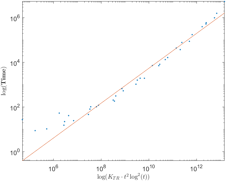
For the computational time complexity of algorithm 1, from section 2.3, we know it is of order 𝒪⁡(KT​R⋅(t2​log2⁡(t)+N​log2⁡(1ϵ))CLOSE\mathcal{O}(K_{TR}\cdot(t^{2}\log^{2}(t)+N\log^{2}(\frac{1}{\epsilon})). Since N≈(t+1)2N\approx(t+1)^{2} in our setting, it is essentially of order 𝒪⁡(KT​R⋅t2​log2⁡(t))\mathcal{O}(K_{TR}\cdot t^{2}\log^{2}(t)). To confirm this, from each row of table 1, we have degree tt, total number KT​RK_{TR} of iterations, and the Time (in second) to generate data points of the form (KT​R⋅t2​log2⁡(t),Time)(K_{TR}\cdot t^{2}\log^{2}(t),\text{Time}). Then, we use log-log plot to show all data points and use linear fitting to fit the data points. The result is plotted in fig. 2, where we can see the log-log plot of the data points is close to the fitted straight line. This confirms that the computational time complexity of algorithm 1 does follow the order of 𝒪⁡(KT​R⋅t2​log2⁡(t))\mathcal{O}(K_{TR}\cdot t^{2}\log^{2}(t)).

Refer to caption
Figure 2: The log-log plot of Time vs. KT​R⋅t2​log2⁡(t)K_{TR}\cdot t^{2}\log^{2}(t). Blue dots are data points of (KT​R⋅t2​log2⁡(t),Time)(K_{TR}\cdot t^{2}\log^{2}(t),\text{Time}) from table 1. Red line is the fitted linear line.

3.3 Spherical tt-designs for function approximation

With the obtained spherical tt-design point sets, we can use it to approximate function as their discrete samples. We demonstrate below how this can be done for a special function class of function, the Wendland functions, defined on the sphere.

A spherical signal is typically sampled from a function f:𝕊2→ℂf:\mathbb{S}^{2}\rightarrow\mathbb{C} on certain point set XN={𝒙i|i∈[N]}X_{N}=\{\bm{x}_{i}\,|\,i\in[N]\}, that is, one only has the sample points {(𝒙i,f⁡(𝒙i))|i∈[N]}\{(\bm{x}_{i},f(\bm{x}_{i}))\,|\,i\in[N]\}. Note that XNX_{N} is not necessarily a spherical tt-design point set. We would like to see how well it can be approximated by a polynomial space ΠT\Pi_{T}. This is equivalent to finding an fT∈ΠTf_{T}\in\Pi_{T} that solves the minimization problem: fT=arg⁡minp∈ΠT​‖f|XN−p|XN‖,f_{T}=\arg\min_{p\in\Pi_{T}}\|f|_{X_{N}}-p|_{X_{N}}\|, where f|XN:=𝒇:=[f⁡(𝒙1),…,f⁡(𝒙N)]⊤f|_{X_{N}}:=\bm{f}:=[f(\bm{x}_{1}),\ldots,f(\bm{x}_{N})]^{\top}. Then we have f=fT+gf=f_{T}+g with g=f−fTg=f-f_{T} being its residual. Note that fT=∑(ℓ,m)∈ℐTc^ℓm​Yℓmf_{T}=\sum_{(\ell,m)\in\mathcal{I}_{T}}\hat{c}_{\ell}^{m}Y_{\ell}^{m} for some 𝒄^:=(c^ℓm)(ℓ,m)∈ℐT\bm{\hat{c}}:=(\hat{c}_{\ell}^{m})_{(\ell,m)\in\mathcal{I}_{T}}. Hence, fT|XN=:𝒇T=𝒀T​(XN)​𝒄^f_{T}|_{X_{N}}=:\bm{f}_{T}=\bm{Y}_{T}(X_{N})\bm{\hat{c}}. The minimization problem is equivalent to

min𝒄^⁡∥𝒇−𝒀T​𝒄^∥,\displaystyle\min_{\bm{\hat{c}}}\lVert\bm{f}-\bm{Y}_{T}\bm{\hat{c}}\rVert, (25)

which can be solved by the least square method. In fact, to find 𝒄^\bm{\hat{c}} such that 𝒀T​𝒄^=𝒇\bm{Y}_{T}\bm{\hat{c}}=\bm{f}, one usually uses a diagonal matrix 𝑾=diag⁡(w1,…,wN)\bm{W}=\diag(w_{1},\ldots,w_{N}) from some weight 𝐰:=w|XN:={w1,…,wN}\mathbf{w}:=w|_{X_{N}}:=\{w_{1},\ldots,w_{N}\} for the purpose of preconditioning. Define b:=𝒀T⋆​𝑾​𝒇b:=\bm{Y}_{T}^{\star}\bm{W}\bm{f} and matrix A=𝒀T⋆​𝑾​𝒀TA=\bm{Y}_{T}^{\star}\bm{W}\bm{Y}_{T}. Then, 𝒀T​𝒄^=𝒇\bm{Y}_{T}\bm{\hat{c}}=\bm{f} can be solved by the normal equation: A​𝒄^=bA\bm{\hat{c}}=b, which can be done by the conjugate gradient (CG) method. See algorithm 3. We remark that we do not need to form A=𝒀T⋆​𝑾​𝒀TA=\bm{Y}_{T}^{\star}\bm{W}\bm{Y}_{T} explicitly but simply the matrix-vector realization A​𝒄^A\bm{\hat{c}}, which can be done fast through 𝒀T⋆​(𝑾⁡(𝒀T​𝒄^))\bm{Y}_{T}^{\star}(\bm{W}(\bm{Y}_{T}\bm{\hat{c}})) using the fast spherical harmonic transforms that we discussed in section 2.3.

Algorithm 3 Projection by Conjugate Gradient Algorithm
0:  TT: polynomial degree; XNX_{N}: spherical point set; 𝐰\mathbf{w}: weights of XNX_{N}; KmaxK_{\max}: maximum iterations; ε\varepsilon: termination tolerance; Initialize x=0x=0, k=0k=0, r0=b=𝒀T⋆​𝑾​𝒇r_{0}=b=\bm{Y}_{T}^{\star}\bm{W}\bm{f}, A=𝒀T⋆​𝑾​𝒀TA=\bm{Y}_{T}^{\star}\bm{W}\bm{Y}_{T} with 𝑾=diag⁡(𝐰)\bm{W}=\diag(\mathbf{w}).
1:  while ∥rk+1∥>ε\lVert r_{k+1}\rVert>\varepsilon and k≤Kmaxk\leq K_{\max} do
2:   if k=0k=0 then
3:    p1=r0p_{1}=r_{0}
4:   else
5:    pk+1=rk+∥rk∥2∥rk−1∥2​pkp_{k+1}=r_{k}+\frac{\lVert r_{k}\rVert^{2}}{\lVert r_{k-1}\rVert^{2}}p_{k}
6:   end if
7:   Compute α=∥rk∥2pk+1⊤​A​pk+1\alpha=\frac{\lVert r_{k}\rVert^{2}}{p_{k+1}^{\top}Ap_{k+1}}. Set xk+1=xk+α​pk+1x_{k+1}=x_{k}+\alpha p_{k+1} and rk+1=rk−α​A​pk+1r_{k+1}=r_{k}-\alpha Ap_{k+1}.
8:   k=k+1k=k+1
9:  end while
9:  𝒄^=:x∗∈ℂ(T+1)2\bm{\hat{c}}=:x^{*}\in\mathbb{C}^{(T+1)^{2}}.

In what follows, we set the maximum iterations Kmax=1000K_{\max}=1000 and termination tolerance ε=2.2204​E-16\varepsilon=2.2204\text{E-16} in algorithm 3. We use the relative projection l2l_{2}-error (with Euclidean norm), i.e., e​r​r​(f,fT):=∥𝒇−𝒇T∥∥𝒇∥err(f,f_{T}):=\frac{\lVert\bm{f}-\bm{f}_{T}\rVert}{\lVert\bm{f}\rVert}, to measure how good the approximation is under different kinds of point sets. We demonstrate our results with ff to be the combinations of normalized Wendland functions, which are a family of compactly supported radial basis functions (RBF). Let (ξ)+:=max⁡{ξ,0}(\xi)_{+}:=\max\{\xi,0\} for ξ∈ℝ\xi\in\mathbb{R}. The original Wendland functions are

ϕ~k​(ξ):={(1−ξ)+2,k=0,(1−ξ)+4​(4​ξ+1),k=1,(1−t)+6​(35​ξ2+18​ξ+3)/3,k=2,(1−ξ)+8​(32​ξ3+25​ξ2+8​ξ+1),k=3,(1−ξ)+10​(429​ξ4+450​ξ3+210​ξ2+50​ξ+5)/5,k=4.\tilde{\phi}_{k}(\xi):=\begin{cases}(1-\xi)_{+}^{2},&k=0,\\[2.84526pt] (1-\xi)_{+}^{4}(4\xi+1),&k=1,\\[2.84526pt] \displaystyle(1-t)_{+}^{6}(35\xi^{2}+18\xi+3)/3,&k=2,\\[2.84526pt] (1-\xi)_{+}^{8}(32\xi^{3}+25\xi^{2}+8\xi+1),&k=3,\\[2.84526pt] \displaystyle(1-\xi)_{+}^{10}(429\xi^{4}+450\xi^{3}+210\xi^{2}+50\xi+5)/5,&k=4.\end{cases}

The normalized (equal area) Wendland functions are ϕk​(ξ):=ϕ~k​(ξΔk)\phi_{k}(\xi):=\tilde{\phi}_{k}\Bigl(\frac{\xi}{\Delta_{k}}\Bigr) with Δk:=(3​k+3)​Γ​(k+12)2​Γ​(k+1)\Delta_{k}:=\frac{(3k+3)\Gamma(k+\frac{1}{2})}{2\>\Gamma(k+1)} for k≥0k\geq 0. The Wendland functions ϕk​(ξ)\phi_{k}(\xi) pointwise converge to Guassian when k→∞k\to\infty, refer to [11]. Thus the main changes as kk increases is the smoothness of ff. Let 𝒛1:=(1,0,0),𝒛2:=(−1,0,0),𝒛3:=(0,1,0),𝒛4:=(0,−1,0),𝒛5:=(0,0,1),𝒛6:=(0,0,−1)\bm{z}_{1}:=(1,0,0),\bm{z}_{2}:=(-1,0,0),\bm{z}_{3}:=(0,1,0),\bm{z}_{4}:=(0,-1,0),\bm{z}_{5}:=(0,0,1),\bm{z}_{6}:=(0,0,-1) be regular octahedron vertices and define ([20])

fk​(𝒙):=∑i=16ϕk​(‖𝒛i−𝒙‖),k≥0.f_{k}(\bm{x}):=\sum_{i=1}^{6}\phi_{k}(\|\bm{z}_{i}-\bm{x}\|),\quad k\geq 0. (26)

The function fkf_{k} are in Wk+32​(𝕊2)W^{k+\frac{3}{2}}(\mathbb{S}^{2}), where Wτ(𝕊2):={f∈L2(𝕊2):∑ℓ=0∞∑|m|≤ℓ(1+ℓ)2​τ|f^ℓm|2}<∞}W^{\tau}(\mathbb{S}^{2}):=\{f\in L_{2}(\mathbb{S}^{2}):\sum_{\ell=0}^{\infty}\sum_{\lvert m\rvert\leq\ell}(1+\ell)^{2\tau}\lvert\hat{f}_{\ell}^{m}\rvert^{2}\}<\infty\} is the Sobolev space with smooth parameter τ>1\tau>1. The function fkf_{k} has limited smoothness at the centers 𝒛i\bm{z}_{i} and at the boundary of each cap with center 𝒛i\bm{z}_{i}. These features make fkf_{k} relatively difficult to approximate in these regions, especially for small kk.

For all initial point sets SP, UD, IV, HL, and their final point sets SPD, SUD, SID, SHD of spherical tt-designs with t=t⁡(N)t=t(N) being determined in section 3, we set the input polynomial degree T=t2T=\frac{t}{2} and (equal) weight 𝐰≡4​πN\mathbf{w}\equiv\frac{4\pi}{N} in algorithm 3. Then for degree t≈200t\approx 200 and N≈(t+1)2N\approx(t+1)^{2}, we show the projection errors e​r​r​(fk,fT)err(f_{k},f_{T}) in table 2 of the five RBF functions f0,…,f4f_{0},\ldots,f_{4} defined in (26). We can see that the order of the errors decreases significantly from −4-4 up to −11-11 with respect to kk in fkf_{k} for each of the final spherical tt-design point sets, while the order of the errors decreases from −4-4 up to −9-9 for the initial point sets. This experiment demonstrates the superiority of spherical tt-designs over normal structure point sets in terms of function approximation.

Table 2: Relative l2l_{2}-errors e​r​r​(fk,fT)err(f_{k},f_{T}) for Wendland functions f0,…,f4f_{0},\ldots,f_{4} approximated by ΠT\Pi_{T} functions for T=t2T=\frac{t}{2} and 𝐰≡4​πN\mathbf{w}\equiv\frac{4\pi}{N} in algorithm 3 with different point sets.
tt NN QNQ_{N} f0f_{0} f1f_{1} f2f_{2} f3f_{3} f4f_{4}
200 40401 SP 5.64E-04 3.19E-06 5.25E-08 3.39E-09 3.21E-09
200 40401 SPD 5.78E-04 3.20E-06 5.25E-08 1.69E-09 8.92E-11
200 40401 UD 6.09E-04 3.07E-06 8.50E-08 8.71E-08 8.53E-08
200 40401 SUD 6.99E-04 3.51E-06 5.63E-08 1.79E-09 1.07E-10
201 40962 IV 8.12E-04 3.32E-06 5.28E-08 4.57E-09 6.10E-08
201 40962 SID 6.15E-04 3.11E-06 5.08E-08 1.64E-09 8.74E-11
220 49152 HL 5.98E-04 2.28E-06 3.18E-08 8.68E-09 8.28E-09
220 49152 SHD 5.98E-04 2.28E-06 3.04E-08 8.11E-10 3.59E-11

4 Spherical framelets from spherical tt-designs

In this section, we detail the construction and characterizations of the (semi-discrete) spherical framelet systems based on the spherical tt-designs. A truncated system is then introduced and the fast spherical framelet transforms in terms of the filter banks and the fast spherical harmonic transforms are then developed.

4.1 Construction and characterizations

Following the setting of the paper by Wang and Zhuang [52] on framelets defined on manifolds, we first define (semi-discrete) framelet system on the sphere. Let functions Ψ:={α;β1,…,βn}⊂L1​(ℝ)\Psi:=\{\alpha;\beta_{1},\ldots,\beta_{n}\}\subset L^{1}(\mathbb{R}) be associated with a filter bank η:={a;b1,…,bn}⊂l1​(ℤ):={h={hk}k∈ℤ⊂ℂ|∑k∈ℤ|hk|<∞}\eta:=\{a;b_{1},\ldots,b_{n}\}\subset l_{1}(\mathbb{Z}):=\{h=\{h_{k}\}_{k\in\mathbb{Z}}\subset\mathbb{C}\,|\,\sum_{k\in\mathbb{Z}}\lvert h_{k}\rvert<\infty\} with the following relations

α^​(2​ξ)=a^​(ξ)​α^​(ξ),β^s​(2​ξ)=b^s​(ξ)​α^​(ξ),ξ∈ℝ,s∈[n],\hat{\alpha}(2\xi)=\hat{a}(\xi)\hat{\alpha}(\xi),\quad\hat{\beta}_{s}(2\xi)=\hat{b}_{s}(\xi)\hat{\alpha}(\xi),\quad\xi\in\mathbb{R},\,s\in[n], (27)

where for a function f∈L1​(ℝ)f\in L^{1}(\mathbb{R}), its Fourier transform f^\hat{f} is defined by f^​(ξ):=∫ℝf⁡(x)​e−2​π​i​x​ξ​𝑑x\hat{f}(\xi):=\int_{\mathbb{R}}f(x)e^{-2\pi\mathrm{i}x\xi}dx, and for a filter (mask) h={hk}k∈ℤ⊂ℂh=\{h_{k}\}_{k\in\mathbb{Z}}\subset\mathbb{C}, its Fourier series h^\hat{h} is defined by h^​(ξ):=∑k∈ℤhk​e−2​π​i​k​ξ\hat{h}(\xi):=\sum_{k\in\mathbb{Z}}h_{k}\mathrm{e}^{-2\pi\mathrm{i}k\xi}, for ξ∈ℝ\xi\in\mathbb{R}. The first equation of eq. 27 is said to be the refinement equation with α\alpha being the refinable function associated with the refinement mask aa (low-pass filter). The functions βs\beta_{s} are framelet generators associated with framelet masks bsb_{s} (high-pass filter) for s∈[n]s\in[n], which can be derived by extension principles [17, 41].

A quadrature (cubature) rule QNj=(XNj,𝐰j)Q_{N_{j}}=(X_{N_{j}},\mathbf{w}_{j}) on 𝕊2\mathbb{S}^{2} at scale jj is a collection QNj:={(𝒙j,k,wj,k)|k∈[Nj]}⊂𝕊2×ℝQ_{N_{j}}:=\{(\bm{x}_{j,k},w_{j,k})\,|\,k\in[N_{j}]\}\subset\mathbb{S}^{2}\times\mathbb{R} of point set XNj:={𝒙j,k|k∈[Nj]}X_{N_{j}}:=\{\bm{x}_{j,k}\,|\,k\in[N_{j}]\} and weight 𝐰j:={wj,k|k∈[Nj]}\mathbf{w}_{j}:=\{w_{j,k}\,|\,k\in[N_{j}]\}, where NjN_{j} is the number of points at scale jj. We said that the quadrature rule QNjQ_{N_{j}} is polynomial-exact up to degree tj∈ℕ0t_{j}\in\mathbb{N}_{0} if ∑k=1Njwj,k​p​(𝒙j,k)=∫𝕊2f⁡(𝒙)​d​μ2​(𝒙)\sum_{k=1}^{N_{j}}w_{j,k}p(\bm{x}_{j,k})=\int_{\mathbb{S}^{2}}f(\bm{x})\mathrm{d}\mu_{2}(\bm{x}) for all p∈Πtjp\in\Pi_{t_{j}}. We call such a QNj=:QNj,tjQ_{N_{j}}=:Q_{N_{j},t_{j}} to be a polynomial-exact quadrature rule of degree tjt_{j}. The spherical tt-design XN={𝒙1,…,𝒙N}X_{N}=\{\bm{x}_{1},\ldots,\bm{x}_{N}\} forms a polynomial-exact quadrature rule QN,t:=(XN,𝐰)Q_{N,t}:=(X_{N},\mathbf{w}) of degree tt with weight 𝐰≡4​πN\mathbf{w}\equiv\frac{4\pi}{N}.

Now given a sequence 𝒬:={QNj,tj}j≥J\mathcal{Q}:=\{Q_{N_{j},t_{j}}\}_{j\geq J} of polynomial-exact quadrature rules, we can define spherical framelets φj,k\varphi_{j,k} and ψj,k(s)\psi_{j,k}^{(s)} for s∈[n]s\in[n] as follows:

φj,k​(𝒙)\displaystyle\varphi_{j,k}(\bm{x}) :=wj,k​∑ℓ=0∞∑m=−ℓℓα^​(λℓ,mtj)​Yℓm​(𝒙j,k)¯​Yℓm​(𝒙),\displaystyle:=\sqrt{w_{j,k}}\sum_{\ell=0}^{\infty}\sum_{m=-\ell}^{\ell}\hat{\alpha}(\frac{\lambda_{\ell,m}}{t_{j}})\overline{Y_{\ell}^{m}(\bm{x}_{j,k})}Y_{\ell}^{m}(\bm{x}), (28)
ψj,k(s)​(𝒙)\displaystyle\psi_{j,k}^{(s)}(\bm{x}) :=wj+1,k​∑ℓ=0∞∑m=−ℓℓβs^​(λℓ,mtj)​Yℓm​(𝒙j+1,k)¯​Yℓm​(𝒙),\displaystyle:=\sqrt{w_{j+1,k}}\sum_{\ell=0}^{\infty}\sum_{m=-\ell}^{\ell}\hat{\beta_{s}}(\frac{\lambda_{\ell,m}}{t_{j}})\overline{Y_{\ell}^{m}(\bm{x}_{j+1,k})}Y_{\ell}^{m}(\bm{x}), (29)

for 𝒙∈𝕊2\bm{x}\in\mathbb{S}^{2}, where in this paper, we set λℓ,m=ℓ\lambda_{\ell,m}=\ell. The (semi-discrete) spherical framelet system ℱJ​(Ψ,𝒬)\mathcal{F}_{J}(\Psi,\mathcal{Q}) starting at a scale J∈ℤJ\in\mathbb{Z} is then defined to be

ℱJ(Ψ,𝒬):={φJ,k:k∈[NJ]}∪{ψj,k(s):k∈[Nj+1],s∈[n]}j=J∞.\displaystyle\mathcal{F}_{J}(\Psi,\mathcal{Q}):=\{\varphi_{J,k}:k\in[N_{J}]\}\cup\{\psi_{j,k}^{(s)}:k\in[N_{j+1}],s\in[n]\}_{j=J}^{\infty}. (30)

By [52, Corollary 2.6], we immediately have the following characterization result for the system ℱJ​(Ψ,𝒬)\mathcal{F}_{J}(\Psi,\mathcal{Q}) to be a tight frame for L2​(𝕊2)L^{2}(\mathbb{S}^{2}).

Theorem 4.

Let α∈L1​(ℝ)\alpha\in L^{1}(\mathbb{R}) be a band-limited function such that supp⁡α^⊆[0,12]\supp\hat{\alpha}\subseteq[0,\frac{1}{2}] and Ψ:={α;βs,…,βn}⊂L1​(ℝ)\Psi:=\{\alpha;\beta_{s},\ldots,\beta_{n}\}\subset L^{1}(\mathbb{R}) be a set of functions associating with a filter bank η:={a;b1,…,bn}⊂l1​(ℤ)\eta:=\{a;b_{1},\ldots,b_{n}\}\subset l_{1}(\mathbb{Z}) as in eq. 27 . Let j∈ℤj\in\mathbb{Z} and QNj,tj={(𝐱j,k,wj,k≡4​πNj)|k∈[Nj]}Q_{N_{j},t_{j}}=\{(\bm{x}_{j,k},w_{j,k}\equiv\frac{4\pi}{N_{j}})\,|\,k\in[N_{j}]\} be the quadrature rule determined by a spherical tjt_{j}-design XNj={𝐱j,1,…,𝐱j,Nj}⊂𝕊2X_{N_{j}}=\{\bm{x}_{j,1},\ldots,\bm{x}_{j,N_{j}}\}\subset\mathbb{S}^{2} satisfying tj+1=2​tjt_{j+1}=2t_{j}. Define ℱJ​(Ψ,𝒬)\mathcal{F}_{J}(\Psi,\mathcal{Q}) as in (30). Let J0∈ℤJ_{0}\in\mathbb{Z} be fixed. Then the following are equivalent.

  1. (i)

    The framelet system ℱJ​(Ψ,𝒬)\mathcal{F}_{J}(\Psi,\mathcal{Q}) is a tight frame for L2​(𝕊2)L^{2}(\mathbb{S}^{2}) for all J≥J0J\geq J_{0}, that is, f=∑k=1NJ⟨f,φJ,k⟩​φJ,k+∑j=J∞∑k=1Nj+1∑s=1n⟨f,ψj,k(s)⟩​ψj,k(s)f=\sum_{k=1}^{N_{J}}\langle f,\varphi_{J,k}\rangle\varphi_{J,k}+\sum_{j=J}^{\infty}\sum_{k=1}^{N_{j+1}}\sum_{s=1}^{n}\langle f,\psi_{j,k}^{(s)}\rangle\psi_{j,k}^{(s)} for all f∈L2​(𝕊2)f\in L^{2}(\mathbb{S}^{2}) and J≥J0J\geq J_{0},

  2. (ii)

    The generators in Ψ\Psi satisfy

    limj→∞|α^​(λℓ,mtj)|=1,ℓ≥0,|m|≤ℓ,\displaystyle\lim_{j\to\infty}\lvert\hat{\alpha}(\frac{\lambda_{\ell,m}}{t_{j}})\rvert=1,\quad\ell\geq 0,\lvert m\rvert\leq\ell, (31)
    |α^​(λℓ,mtj+1)|2=|α^​(λℓ,mtj)|2+∑s=1n|β^s​(λℓ,mtj)|2,ℓ≥0,|m|≤ℓ,j≥J0.\displaystyle\lvert\hat{\alpha}(\frac{\lambda_{\ell,m}}{t_{j+1}})\rvert^{2}=\lvert\hat{\alpha}(\frac{\lambda_{\ell,m}}{t_{j}})\rvert^{2}+\sum_{s=1}^{n}\lvert\hat{\beta}_{s}(\frac{\lambda_{\ell,m}}{t_{j}})\rvert^{2},\quad\ell\geq 0,\lvert m\rvert\leq\ell,j\geq J_{0}. (32)
  3. (iii)

    The refinable function α\alpha satisfies eq. 31 and the filters in η\eta satisfy

    |a^​(λℓ,mtj)|2+∑s=1n|b^s​(λℓ,mtj)|2=1∀ℓ,m∈ℐαj,∀j≥J0+1,\displaystyle\lvert\hat{a}(\frac{\lambda_{\ell,m}}{t_{j}})\rvert^{2}+\sum_{s=1}^{n}\lvert\hat{b}_{s}(\frac{\lambda_{\ell,m}}{t_{j}})\rvert^{2}=1\quad\forall\ell,m\in\mathcal{I}_{\alpha}^{j},\forall j\geq J_{0}+1, (33)

    where ℐαj:={ℓ∈ℕ0,|m|≤ℓ:α^(λℓ,mtj)≠0}\mathcal{I}_{\alpha}^{j}:=\{\ell\in\mathbb{N}_{0},\lvert m\rvert\leq\ell:\hat{\alpha}(\frac{\lambda_{\ell,m}}{t_{j}})\neq 0\}.

Proof.

We only need to show that the product rule holds for the spherical harmonics YℓmY_{\ell}^{m} since all other conditions in [52, Corollary 2.6] hold. We next use induction to prove that the product of two spherical harmonics YℓmY_{\ell}^{m} and Yℓ′m′Y_{\ell^{\prime}}^{m^{\prime}} is in Πℓ+ℓ′\Pi_{\ell+\ell^{\prime}}, that is, Yℓm​Yℓ′m′∈Πℓ+ℓ′Y_{\ell}^{m}Y_{\ell^{\prime}}^{m^{\prime}}\in\Pi_{\ell+\ell^{\prime}} and it can be written as the linear combination of {Yℓ~m~:ℓ~≤ℓ+ℓ′,|m~|≤ℓ~}\{Y_{\tilde{\ell}}^{\tilde{m}}:\tilde{\ell}\leq\ell+\ell^{\prime},\lvert\tilde{m}\rvert\leq\tilde{\ell}\}. By the definition of YℓmY_{\ell}^{m} in (8), it sufficient to show that the product of two associate Legendre polynomials Pℓm​(z)P_{\ell}^{m}(z) and Pℓ′m′​(z)P_{\ell^{\prime}}^{m^{\prime}}(z) can be written as the linear combination of {Pℓ~m~(z):ℓ~≤ℓ+ℓ′,m=0,…,ℓ}\{P_{\tilde{\ell}}^{\tilde{m}}(z):\tilde{\ell}\leq\ell+\ell^{\prime},m=0,\ldots,\ell\} for z∈[−1,1]z\in[-1,1]. That is

Pℓm​(z)​Pℓ′m′​(z)=∑0≤ℓ~≤ℓ+ℓ′∑0≤m≤ℓ~cℓ~m​Pℓ~m​(z),z∈[−1,1].\displaystyle P_{\ell}^{m}(z)P_{\ell^{\prime}}^{m^{\prime}}(z)=\sum_{0\leq\tilde{\ell}\leq\ell+\ell^{\prime}}\sum_{0\leq m\leq\tilde{\ell}}c_{\tilde{\ell}}^{m}P_{\tilde{\ell}}^{m}(z),\quad z\in[-1,1]. (34)

We prove it by mathematical induction on ℓ+ℓ′\ell+\ell^{\prime}. We omit zz in Pℓm​(z),Pℓ′m′​(z)P_{\ell}^{m}(z),P_{\ell^{\prime}}^{m^{\prime}}(z) and Pℓ~m~​(z)P_{\tilde{\ell}}^{\tilde{m}}(z) for convenience.

For ℓ+ℓ′=0\ell+\ell^{\prime}=0, the equation (34) trivially holds. Suppose eq. 34 holds for ℓ+ℓ′=k∈ℕ0\ell+\ell^{\prime}=k\in\mathbb{N}_{0}. We next prove for ℓ+ℓ′=k+1\ell+\ell^{\prime}=k+1 the equation (34) holds. Without loss of generality, we can assume ℓ≥2\ell\geq 2 (otherwise, we can prove it for ℓ=0,1\ell=0,1 directly). By the recurrence formula of associated Legendre polynomial: (ℓ−m+1)​Pℓ+1m​(z)=(2​ℓ+1)​z​Pℓm​(z)−(ℓ+m)​Pℓ−1m​(z)(\ell-m+1)P_{\ell+1}^{m}(z)=(2\ell+1)zP_{\ell}^{m}(z)-(\ell+m)P_{\ell-1}^{m}(z), we have

Pℓm​Pℓ′m′=2​ℓ−1ℓ−m​z​Pℓ−1m​Pℓ′m′−ℓ−1+mℓ−m​Pℓ−2m​Pℓ′m′.\displaystyle P_{\ell}^{m}P_{\ell^{\prime}}^{m^{\prime}}=\frac{2\ell-1}{\ell-m}zP_{\ell-1}^{m}P_{\ell^{\prime}}^{m^{\prime}}-\frac{\ell-1+m}{\ell-m}P_{\ell-2}^{m}P_{\ell^{\prime}}^{m^{\prime}}. (35)

From the inductive hypothesis and P10​(z)=zP_{1}^{0}(z)=z for z∈[−1,1]z\in[-1,1], eq. 35 can be written as

Pℓm​Pℓ′m′\displaystyle P_{\ell}^{m}P_{\ell^{\prime}}^{m^{\prime}} =z​∑ℓ~≤k∑m~≤ℓ~cℓ~m~​Pℓ~m~+∑ℓ~≤k−1∑m~≤ℓ~dℓ~m~​Pℓ~m~\displaystyle=z\sum_{\tilde{\ell}\leq k}\sum_{\tilde{m}\leq\tilde{\ell}}c_{\tilde{\ell}}^{\tilde{m}}P_{\tilde{\ell}}^{\tilde{m}}+\sum_{\tilde{\ell}\leq k-1}\sum_{\tilde{m}\leq\tilde{\ell}}d_{\tilde{\ell}}^{\tilde{m}}P_{\tilde{\ell}}^{\tilde{m}} (36)
=∑ℓ~≤k−1∑m~≤ℓ~cℓ~m~​P10​Pℓ~m~+∑m~≤kckm~​P10​Pkm~+∑ℓ~≤k−1∑m~≤ℓ~dℓ~m~​Pℓ~m~\displaystyle=\sum_{\tilde{\ell}\leq k-1}\sum_{\tilde{m}\leq\tilde{\ell}}c_{\tilde{\ell}}^{\tilde{m}}P_{1}^{0}P_{\tilde{\ell}}^{\tilde{m}}+\sum_{\tilde{m}\leq k}c_{k}^{\tilde{m}}P_{1}^{0}P_{k}^{\tilde{m}}+\sum_{\tilde{\ell}\leq k-1}\sum_{\tilde{m}\leq\tilde{\ell}}d_{\tilde{\ell}}^{\tilde{m}}P_{\tilde{\ell}}^{\tilde{m}}
=∑ℓ~≤k∑m~≤ℓ~eℓ~m~​Pℓ~m~+∑ℓ~≤k+1∑m~≤ℓ~hℓ~m~​Pℓ~m~+∑ℓ~≤k−1∑m~≤ℓ~dℓ~m~​Pℓ~m~\displaystyle=\sum_{\tilde{\ell}\leq k}\sum_{\tilde{m}\leq\tilde{\ell}}e_{\tilde{\ell}}^{\tilde{m}}P_{\tilde{\ell}}^{\tilde{m}}+\sum_{\tilde{\ell}\leq k+1}\sum_{\tilde{m}\leq\tilde{\ell}}h_{\tilde{\ell}}^{\tilde{m}}P_{\tilde{\ell}}^{\tilde{m}}+\sum_{\tilde{\ell}\leq k-1}\sum_{\tilde{m}\leq\tilde{\ell}}d_{\tilde{\ell}}^{\tilde{m}}P_{\tilde{\ell}}^{\tilde{m}}
=∑ℓ~≤k+1∑m~≤ℓ~aℓ~m~​Pℓ~m~,\displaystyle=\sum_{\tilde{\ell}\leq k+1}\sum_{\tilde{m}\leq\tilde{\ell}}a_{\tilde{\ell}}^{\tilde{m}}P_{\tilde{\ell}}^{\tilde{m}},

where we use P10​Pℓm=12​ℓ+1​[(ℓ−m+1)​Pℓ+1m+(ℓ+m)​Pℓ−1m]P_{1}^{0}P_{\ell}^{m}=\frac{1}{2\ell+1}[(\ell-m+1)P_{\ell+1}^{m}+(\ell+m)P_{\ell-1}^{m}] from the recurrence relation, and aℓ~m~,cℓ~m~,dℓ~m~,eℓ~m~,hℓ~m~a_{\tilde{\ell}}^{\tilde{m}},c_{\tilde{\ell}}^{\tilde{m}},d_{\tilde{\ell}}^{\tilde{m}},e_{\tilde{\ell}}^{\tilde{m}},h_{\tilde{\ell}}^{\tilde{m}} are coefficients in different components. That is, eq. 34 holds for ℓ+ℓ′=k+1\ell+\ell^{\prime}=k+1.

Therefore, by mathematical induction, for every ℓ,ℓ′∈ℕ0\ell,\ell^{\prime}\in\mathbb{N}_{0}, eq. 34 holds for z∈[−1,1]z\in[-1,1]. Hence, we complete the proof.

Remark 5.

By the contract rule and the Wigner 3​j3j-symbols [50], the product rule holds but it is hard to tell what is the resulted degree of the product of two spherical harmonics. Besides, it is not explicitly proved in [52] for the product rule of spherical harmonics. Hence, we provide an elementary proof here. By the product rule, given a spherical tt-design XN={𝐱1,…,𝐱N}X_{N}=\{\bm{x}_{1},\ldots,\bm{x}_{N}\}, we immediately have

4​πN​∑i=1NYℓm​(𝒙i)​Yℓ′m′​(𝒙i)¯=⟨Yℓm,Yℓ′m′⟩=δℓ​ℓ′​δm​m′,\displaystyle\frac{4\pi}{N}\sum_{i=1}^{N}Y_{\ell}^{m}(\bm{x}_{i})\overline{Y_{\ell^{\prime}}^{m^{\prime}}(\bm{x}_{i})}=\langle Y_{\ell}^{m},Y_{\ell^{\prime}}^{m^{\prime}}\rangle=\delta_{\ell\ell^{\prime}}\delta_{mm^{\prime}}, (37)

for all ℓ+ℓ′≤t\ell+\ell^{\prime}\leq t, |m|≤ℓ,|m′|≤ℓ′|m|\leq\ell,|m^{\prime}|\leq\ell^{\prime}. This implies 4​πN​𝐘⌊t/2⌋⋆​(XN)​𝐘⌊t/2⌋​(XN)=𝐈(⌊t/2⌋+1)2\frac{4\pi}{N}\bm{Y}_{\lfloor t/2\rfloor}^{\star}(X_{N})\bm{Y}_{\lfloor t/2\rfloor}(X_{N})=\mathbf{I}_{(\lfloor t/2\rfloor+1)^{2}} with 𝐈k\mathbf{I}_{k} being the identity matrix of size kk.

4.2 Truncated spherical framelet systems

In practice, the infinite system ℱJ0​(Ψ,𝒬)\mathcal{F}_{J_{0}}(\Psi,\mathcal{Q}) in 4 needs to be truncated at certain scale J1≥J0J_{1}\geq J_{0} and the filter bank η={a;b1,…,bn}\eta=\{a;b_{1},\ldots,b_{n}\} plays the key role in the decomposition and reconstruction of a discrete signal on the sphere. Here, we discuss the truncated systems of spherical framelets for practical spherical signal processing.

We first suppose that the filter bank η={a;b1,…,bn}\eta=\{a;b_{1},\ldots,b_{n}\} is designed beforehand that satisfies the partition of unity condition:

|a^​(ξ)|2+∑s∈[n]|b^s​(ξ)|2=1,ξ∈ℝ.\displaystyle|\hat{a}(\xi)|^{2}+\sum_{s\in[n]}|\hat{b}_{s}(\xi)|^{2}=1,\quad\xi\in\mathbb{R}. (38)

For a fixed fine scale J∈ℤJ\in\mathbb{Z}, we set

α^(J+1)​(λℓ,mtJ+1)={1for ​ℓ≤tJ,0for ​ℓ>tJ,\displaystyle\hat{\alpha}^{(J+1)}(\frac{\lambda_{\ell,m}}{t_{J+1}})=\begin{cases}1&\mbox{for }\ell\leq t_{J},\\ 0&\mbox{for }\ell>t_{J},\end{cases} (39)

and following eq. 27, we recursively define α^(j),β^s(j)\hat{\alpha}^{(j)},\hat{\beta}_{s}^{(j)} from α^(j+1)\hat{\alpha}^{(j+1)} by

α^(j)​(λℓ,mtj)=\displaystyle\hat{\alpha}^{(j)}(\frac{\lambda_{\ell,m}}{t_{j}})= α^(j)​(2​λℓ,mtj+1)=a^​(λℓ,mtj+1)​α^(j+1)​(λℓ,mtj+1),\displaystyle\hat{\alpha}^{(j)}(2\frac{\lambda_{\ell,m}}{t_{j+1}})=\hat{a}(\frac{\lambda_{\ell,m}}{t_{j+1}})\hat{\alpha}^{(j+1)}(\frac{\lambda_{\ell,m}}{t_{j+1}}), (40)
β^s(j)​(λℓ,mtj)=\displaystyle\hat{\beta}_{s}^{(j)}(\frac{\lambda_{\ell,m}}{t_{j}})= β^s(j)​(2​λℓ,mtj+1)=b^s​(λℓ,mtj+1)​α^(j+1)​(λℓ,mtj+1),s∈[n],\displaystyle\hat{\beta}_{s}^{(j)}(2\frac{\lambda_{\ell,m}}{t_{j+1}})=\hat{b}_{s}(\frac{\lambda_{\ell,m}}{t_{j+1}})\hat{\alpha}^{(j+1)}(\frac{\lambda_{\ell,m}}{t_{j+1}}),\quad s\in[n], (41)

for jj decreasing from JJ to J0J_{0}. Then, we obtain

Ψ={α(j),βs(j)|j=J0,…,J;s∈[n]}.\displaystyle\Psi=\{\alpha^{(j)},\beta_{s}^{(j)}\,|\,j=J_{0},\ldots,J;s\in[n]\}. (42)

Let 𝒬:=𝒬J0J+1:={QNj,tj:j=J0,…,J+1}\mathcal{Q}:=\mathcal{Q}_{J_{0}}^{J+1}:=\{Q_{N_{j},t_{j}}:j=J_{0},\ldots,J+1\} be the set of polynomial-exact quadrature rules truncated from original infinite sequence of spherical tjt_{j}-designs satisfying tj+1=2​tjt_{j+1}=2t_{j}.

With the above Ψ\Psi and 𝒬\mathcal{Q}, we can define the truncated (semi-discrete) spherical framelet system ℱJ0J​(η,𝒬)\mathcal{F}_{J_{0}}^{J}(\eta,\mathcal{Q}) as

ℱJ0J(η,𝒬):={φJ0,k|k∈[NJ0]}∪{ψj,k(s)|k∈[Nj+1],s∈[n]}j=J0J,\displaystyle\mathcal{F}_{J_{0}}^{J}(\eta,\mathcal{Q}):=\{\varphi_{J_{0},k}\,|\,k\in[N_{J_{0}}]\}\cup\{\psi_{j,k}^{(s)}\,|\,k\in[N_{j+1}],s\in[n]\}_{j=J_{0}}^{J}, (43)

where the φj,k\varphi_{j,k} and ψj,k(s)\psi_{j,k}^{(s)} are modified as

φj,k​(𝒙)\displaystyle\varphi_{j,k}(\bm{x}) :=wj,k​∑(ℓ,m)∈ℐtjα^(j)​(λℓ,mtj)​Yℓm​(𝒙j,k)¯​Yℓm​(𝒙),\displaystyle:=\sqrt{w_{j,k}}\sum_{(\ell,m)\in\mathcal{I}_{t_{j}}}\hat{\alpha}^{(j)}(\frac{\lambda_{\ell,m}}{t_{j}})\overline{Y_{\ell}^{m}(\bm{x}_{j,k})}Y_{\ell}^{m}(\bm{x}), (44)
ψj,k(s)​(𝒙)\displaystyle\psi_{j,k}^{(s)}(\bm{x}) :=wj+1,k​∑(ℓ,m)∈ℐtj+1β^s(j)​(λℓ,mtj)​Yℓm​(𝒙j+1,k)¯​Yℓm​(𝒙).\displaystyle:=\sqrt{w_{j+1,k}}\sum_{(\ell,m)\in\mathcal{I}_{t_{j+1}}}\hat{\beta}_{s}^{(j)}(\frac{\lambda_{\ell,m}}{t_{j}})\overline{Y_{\ell}^{m}(\bm{x}_{j+1,k})}Y_{\ell}^{m}(\bm{x}). (45)

Note that in the notation ℱJ0J​(η,𝒬)\mathcal{F}_{J_{0}}^{J}(\eta,\mathcal{Q}), we emphasize on the role of the filter bank η\eta. The system ℱJ0J​(η,𝒬)\mathcal{F}_{J_{0}}^{J}(\eta,\mathcal{Q}) is completely determined by the filter bank η\eta and the quadrature rules 𝒬\mathcal{Q}. We have the following result regarding the tightness of ℱJ0J​(η,𝒬)\mathcal{F}_{J_{0}}^{J}(\eta,\mathcal{Q}) and its relation to ΠtJ\Pi_{t_{J}}.

Theorem 6.

Let ℱJ0J​(η,𝒬)\mathcal{F}_{J_{0}}^{J}(\eta,\mathcal{Q}) be the truncated spherical framelet system defined as in (43) and assume that the filter bank η\eta satisfies the partition of unity condition (38) with supp⁡a^⊆[0,14]\supp\hat{a}\subseteq[0,\frac{1}{4}] and supp⁡b^s⊆[0,12]\supp\hat{b}_{s}\subseteq[0,\frac{1}{2}] for s∈[n]s\in[n]. Define 𝒱j:=span⁡{φj,k|k∈[Nj]}\mathcal{V}_{j}:=\spn\{\varphi_{j,k}\,|\,k\in[N_{j}]\} and 𝒲j:=span{ψj,k(s)|k∈[Nj+1],s∈[n]}\mathcal{W}_{j}:=\spn\{\psi_{j,k}^{(s)}\,|\,k\in[N_{j+1}],s\in[n]\}. Then the following results hold.

  1. (i)

    ΠtJ=𝒱J+1\Pi_{t_{J}}=\mathcal{V}_{J+1} and thus f=∑k=1NJ+1⟨f,φJ+1,k⟩​φJ+1,kf=\sum_{k=1}^{N_{J+1}}\langle f,\varphi_{J+1,k}\rangle\varphi_{J+1,k} for any f∈ΠtJf\in\Pi_{t_{J}}.

  2. (ii)

    The decomposition and reconstruction relation 𝒱j+1=𝒱j+𝒲j\mathcal{V}_{j+1}=\mathcal{V}_{j}+\mathcal{W}_{j} holds for j=J0,…,Jj=J_{0},\ldots,J.

  3. (iii)

    The truncated spherical framelet system ℱJ0J​(η,𝒬)\mathcal{F}_{J_{0}}^{J}(\eta,\mathcal{Q}) is a tight frame for ΠtJ\Pi_{t_{J}}. That is, for all f∈ΠtJf\in\Pi_{t_{J}}, we have f=∑k=1N0𝓋𝒥0,𝓀​φ𝒥0,𝓀+∑𝒿=𝒥0𝒥∑𝓀=1𝒩𝒿∑𝓈=1𝓃𝓌𝒿,𝓀(𝓈)​ψ𝒿,𝓀(𝓈)f=\sum_{k=1}^{N_{0}}\mathpzc v_{J_{0},k}\varphi_{J_{0},k}+\sum_{j=J_{0}}^{J}\sum_{k=1}^{N_{j}}\sum_{s=1}^{n}\mathpzc w_{j,k}^{(s)}\psi_{j,k}^{(s)}, where 𝓋𝒿,𝓀:=⟨𝒻,φ𝒿,𝓀⟩​ and ​𝓌𝒿,𝓀(𝓈):=⟨𝒻,ψ𝒿,𝓀(𝓈)⟩.\mathpzc v_{j,k}:=\langle f,\varphi_{j,k}\rangle\mbox{ and }\mathpzc w_{j,k}^{(s)}:=\langle f,\psi_{j,k}^{(s)}\rangle.

Proof.

By eq. 39, we have 𝒱J+1⊆ΠtJ\mathcal{V}_{J+1}\subseteq\Pi_{t_{J}}. One the other hand, for f∈ΠtJf\in\Pi_{t_{J}}, we have

f\displaystyle f =∑(ℓ,m)∈ℐtJ+1f^ℓm​Yℓm=∑(ℓ,m)∈ℐtJ+1f^ℓm​|α^(J+1)​(λℓ,mtJ+1)|2​Yℓm.\displaystyle=\sum_{(\ell,m)\in\mathcal{I}_{t_{J+1}}}\hat{f}_{\ell}^{m}Y_{\ell}^{m}=\sum_{(\ell,m)\in\mathcal{I}_{t_{J+1}}}\hat{f}_{\ell}^{m}\lvert\hat{\alpha}^{(J+1)}(\frac{\lambda_{\ell,m}}{t_{J+1}})\rvert^{2}Y_{\ell}^{m}.

We next show that the last equation above implies f=∑k=1NJ+1𝓋𝒥+1,𝓀​φ𝒥+1,𝓀∈𝒱𝒥+1f=\sum_{k=1}^{N_{J+1}}\mathpzc v_{J+1,k}\varphi_{J+1,k}\in\mathcal{V}_{J+1}. In fact, more generally, by the orthogonality of YℓmY_{\ell}^{m}, for any f∈L2​(𝕊2)f\in L^{2}(\mathbb{S}^{2}), we have 𝓋𝒿,𝓀=⟨𝒻,φ𝒿,𝓀⟩=∑(ℓ,𝓂)∈ℐ𝓉𝒿𝒻^ℓ𝓂​α^¯(𝒿)​(λℓ,𝓂𝓉𝒿)​𝓌𝒿,𝓀​𝒴ℓ𝓂​(x𝒿,𝓀)\mathpzc v_{j,k}=\langle f,\varphi_{j,k}\rangle=\sum_{(\ell,m)\in\mathcal{I}_{t_{j}}}\hat{f}_{\ell}^{m}{\bar{\hat{\alpha}}^{(j)}}(\frac{\lambda_{\ell,m}}{t_{j}})\sqrt{w_{j,k}}Y_{\ell}^{m}(\bm{x}_{j,k}). Together with that QNj,tj{Q}_{N_{j},t_{j}} is a polynomial-exact quadrature rule of degree tjt_{j} and α^(j)​(λℓ,mtj)≡0\hat{\alpha}^{(j)}(\frac{\lambda_{\ell,m}}{t_{j}})\equiv 0 for ℓ>tj−1\ell>t_{j-1} in view of eq. 39 and supp⁡a^⊆[0,12]\supp\hat{a}\subseteq[0,\frac{1}{2}], we can deduce that

∑k=1Nj𝓋𝒿,𝓀​φ𝒿,𝓀\displaystyle\sum_{k=1}^{N_{j}}\mathpzc v_{j,k}\varphi_{j,k} =∑(ℓ,m)∈ℐtj∑(ℓ′,m′)∈ℐtjf^ℓm​α^¯(j)​(λℓ,mtj)​α^(j)​(λℓ′,m′tj)​𝒰ℓ,mℓ′,m′​(QNj,tj)​Yℓ′m′\displaystyle=\sum_{(\ell,m)\in\mathcal{I}_{t_{j}}}\sum_{(\ell^{\prime},m^{\prime})\in\mathcal{I}_{t_{j}}}\hat{f}_{\ell}^{m}{\bar{\hat{\alpha}}^{(j)}}(\frac{\lambda_{\ell,m}}{t_{j}}){{\hat{\alpha}}^{(j)}}(\frac{\lambda_{\ell^{\prime},m^{\prime}}}{t_{j}})\mathcal{U}_{\ell,m}^{\ell^{\prime},m^{\prime}}(Q_{N_{j},t_{j}})Y_{\ell^{\prime}}^{m^{\prime}}
=∑(ℓ,m)∈ℐtjf^ℓm​|α^(j)​(λℓ,mtj)|2​Yℓm,\displaystyle=\sum_{(\ell,m)\in\mathcal{I}_{t_{j}}}\hat{f}_{\ell}^{m}\lvert\hat{\alpha}^{(j)}(\frac{\lambda_{\ell,m}}{t_{j}})\rvert^{2}Y_{\ell}^{m},

where we use 𝒰ℓ,mℓ′,m′​(QNj,tj):=∑k=1Njwj,k​Yℓm​(𝒙j,k)​Yℓ′m′​(𝒙j,k)¯=δℓ​ℓ′​δm​m′\mathcal{U}_{\ell,m}^{\ell^{\prime},m^{\prime}}(Q_{N_{j},t_{j}}):=\sum_{k=1}^{N_{j}}{w_{j,k}}Y_{\ell}^{m}(\bm{x}_{j,k})\overline{Y_{\ell^{\prime}}^{m^{\prime}}(\bm{x}_{j,k})}=\delta_{\ell\ell^{\prime}}\delta_{mm^{\prime}}. Item (i) is proved.

For Item (ii), by definition, we obviously have 𝒱j+𝒲j⊆𝒱j+1\mathcal{V}_{j}+\mathcal{W}_{j}\subseteq\mathcal{V}_{j+1}. For the other direction, similarly to above, for any f∈L2​(𝕊2)f\in L^{2}(\mathbb{S}^{2}), we can deduce that ∑k=1Nj+1𝓌𝒿,𝓀(𝓈)​ψ𝒿,𝓀(𝓈)=∑(ℓ,𝓂)∈ℐ𝓉𝒿+1𝒻^ℓ𝓂​|β^𝓈(𝒿)​(λℓ,𝓂𝓉𝒿)|2​𝒴ℓ𝓂\sum_{k=1}^{N_{j+1}}\mathpzc w_{j,k}^{(s)}\psi_{j,k}^{(s)}=\sum_{(\ell,m)\in\mathcal{I}_{t_{j+1}}}\hat{f}_{\ell}^{m}\lvert\hat{\beta}_{s}^{(j)}(\frac{\lambda_{\ell,m}}{t_{j}})\rvert^{2}Y_{\ell}^{m} . Then, by eqs. 40, 41, and 38, we have

∑k=1Nj+1𝓋𝒿+1,𝓀​φ𝒿+1,𝓀\displaystyle\sum_{k=1}^{N_{j+1}}\mathpzc v_{j+1,k}\varphi_{j+1,k} =∑(ℓ,m)∈ℐtj+1f^ℓm​|α^​(λℓ,mtj+1)|2​Yℓm\displaystyle=\sum_{(\ell,m)\in\mathcal{I}_{t_{j+1}}}\hat{f}_{\ell}^{m}\lvert\hat{\alpha}(\frac{\lambda_{\ell,m}}{t_{j+1}})\rvert^{2}Y_{\ell}^{m}
=∑(ℓ,m)∈ℐtj+1f^ℓm​|α^​(λℓ,mtj+1)|2​(|a^​(λℓ,mtj+1)|2+∑s=1n|b^s​(λℓ,mtj+1)|2)​Yℓm\displaystyle=\sum_{(\ell,m)\in\mathcal{I}_{t_{j+1}}}\hat{f}_{\ell}^{m}\lvert\hat{\alpha}(\frac{\lambda_{\ell,m}}{t_{j+1}})\rvert^{2}\left(\lvert\hat{a}(\frac{\lambda_{\ell,m}}{t_{j+1}})\rvert^{2}+\sum_{s=1}^{n}\lvert\hat{b}_{s}(\frac{\lambda_{\ell,m}}{t_{j+1}})\rvert^{2}\right)Y_{\ell}^{m}
=∑(ℓ,m)∈ℐtjf^ℓm​|α^​(λℓ,mtj)|2​Yℓm+∑s=1n∑(ℓ,m)∈ℐtj+1f^ℓm​|β^s​(λℓ,mtj)|2​Yℓm\displaystyle=\sum_{(\ell,m)\in\mathcal{I}_{t_{j}}}\hat{f}_{\ell}^{m}\lvert\hat{\alpha}(\frac{\lambda_{\ell,m}}{t_{j}})\rvert^{2}Y_{\ell}^{m}+\sum_{s=1}^{n}\sum_{(\ell,m)\in\mathcal{I}_{t_{j+1}}}\hat{f}_{\ell}^{m}\lvert\hat{\beta}_{s}(\frac{\lambda_{\ell,m}}{t_{j}})\rvert^{2}Y_{\ell}^{m}
=∑k=1Nj𝓋𝒿,𝓀​φ𝒿,𝓀+∑𝓀=1𝒩𝒿+1∑𝓈=1𝓃𝓌𝒿,𝓀(𝓈)​ψ𝒿,𝓀(𝓈).\displaystyle=\sum_{k=1}^{N_{j}}\mathpzc v_{j,k}\varphi_{j,k}+\sum_{k=1}^{N_{j+1}}\sum_{s=1}^{n}\mathpzc w_{j,k}^{(s)}\psi_{j,k}^{(s)}.

Therefore, we have 𝒱j+1⊆𝒱j+𝒲j\mathcal{V}_{j+1}\subseteq\mathcal{V}_{j}+\mathcal{W}_{j} for all j=0,…,Jj=0,\ldots,J. Item (ii) holds.

Item (iii) directly follows from items (i) and (ii). This completes the proof.

4.3 Fast spherical framelet transforms

We next turn to the fast spherical framelet transforms (SFmTs) for the decomposition and reconstruction of a signal on the sphere 𝕊2\mathbb{S}^{2} using the truncated system ℱJ0J​(η,𝒬)\mathcal{F}_{J_{0}}^{J}(\eta,\mathcal{Q}).

For a vector 𝒄^=(c^ℓm)(ℓ,m)∈ℐtj+1\bm{\hat{c}}=(\hat{c}_{\ell}^{m})_{(\ell,m)\in\mathcal{I}_{t_{j+1}}}, define the downsampling operator ↓j+1\downarrow_{j+1} by 𝒄^↓j:=(c^ℓm)(ℓ,m)∈ℐtj\bm{\hat{c}}\downarrow_{j}:=(\hat{c}_{\ell}^{m})_{(\ell,m)\in\mathcal{I}_{t_{j}}}. Similarly, for a vector 𝒄^=(c^ℓm)(ℓ,m)∈ℐtj\bm{\hat{c}}=(\hat{c}_{\ell}^{m})_{(\ell,m)\in\mathcal{I}_{t_{j}}}, define the upsampling operator ↑j+1\uparrow_{j+1} by 𝒄^↑j+1:=(c^ℓm)(ℓ,m)∈ℐtj+1\bm{\hat{c}}\uparrow_{j+1}:=(\hat{c}_{\ell}^{m})_{(\ell,m)\in\mathcal{I}_{t_{j+1}}} with c^ℓm=0\hat{c}_{\ell}^{m}=0 for ℓ>tj\ell>t_{j}. The symbol ⊙\odot denotes the Hadamard entry-wise product operator.

We have the following theorem regarding the decomposition of reconstruction using the truncated spherical framelet system ℱJ0J​(η,𝒬)\mathcal{F}_{J_{0}}^{J}(\eta,\mathcal{Q}).

Theorem 7.

Given a truncated system ℱJ0J​(η,𝒬)\mathcal{F}_{J_{0}}^{J}(\eta,\mathcal{Q}) as in 6. Define

𝒗j\displaystyle\bm{v}_{j} :=(𝓋𝒿,𝓀)𝓀∈[𝒩𝒿]∈ℂ𝒩𝒿,\displaystyle:=(\mathpzc v_{j,k})_{k\in[N_{j}]}\in\mathbb{C}^{N_{j}}, 𝒘j(s)\displaystyle\bm{w}_{j}^{(s)} :=(𝓌𝒿,𝓀)𝓀∈[𝒩𝒿+1]∈ℂ𝒩𝒿+1,\displaystyle:=(\mathpzc w_{j,k})_{k\in[N_{j+1}]}\in\mathbb{C}^{N_{j+1}}, (46)
𝒂^j\displaystyle\bm{\hat{a}}_{j} :=(a^​(λℓmtj+1))(ℓ,m)∈ℐtj+1,\displaystyle:=(\hat{a}(\frac{\lambda_{\ell}^{m}}{t_{j+1}}))_{(\ell,m)\in\mathcal{I}_{t_{j+1}}}, 𝒃^j(s)\displaystyle\bm{\hat{b}}^{(s)}_{j} :=(b^s​(λℓmtj+1))(ℓ,m)∈ℐtj+1,\displaystyle:=(\hat{b}_{s}(\frac{\lambda_{\ell}^{m}}{t_{j+1}}))_{(\ell,m)\in\mathcal{I}_{t_{j+1}}}, (47)

for j=J0,…,Jj=J_{0},\ldots,J. Let wj:=4​πNjw_{j}:=\frac{4\pi}{N_{j}}. Then, for j=J0,…,Jj=J_{0},\ldots,J, we have the one-level framelet decomposition that obtains {𝐯j,𝐰j(s)|s∈[n]}\{\bm{v}_{j},\bm{w}_{j}^{(s)}\,|\,s\in[n]\} from 𝐯j+1\bm{v}_{j+1}:

𝒗j\displaystyle\bm{v}_{j} =wj𝒀tj[[(wj+1𝒀tj+1⋆𝒗j+1)⊙𝒂^¯j]↓j],\displaystyle={\sqrt{w_{j}}}\bm{Y}_{t_{j}}\left[[(\sqrt{w_{j+1}}\bm{Y}_{t_{j+1}}^{\star}\bm{v}_{j+1})\odot\bm{\bar{\hat{a}}}_{j}]\downarrow_{j}\right], (48)
𝒘j(s)\displaystyle\bm{w}_{j}^{(s)} =wj+1​𝒀tj+1​[(wj+1​𝒀tj+1⋆​𝒗j+1)⊙𝒃^¯j(s)],s∈[n],\displaystyle={\sqrt{w_{j+1}}}\bm{Y}_{t_{j+1}}\left[(\sqrt{w_{j+1}}\bm{Y}_{t_{j+1}}^{\star}\bm{v}_{j+1})\odot\bm{\bar{\hat{b}}}^{(s)}_{j}\right],\quad s\in[n], (49)

and the one-level framelet reconstruction of 𝐯j+1\bm{v}_{j+1} from {𝐯j,𝐰j(s)|s∈[n]}\{\bm{v}_{j},\bm{w}_{j}^{(s)}\,|\,s\in[n]\}:

𝒗j+1\displaystyle\bm{v}_{j+1} =wj+1𝒀tj+1[[wj𝒀tj⋆𝒗j]↑j+1⊙𝒂^j+∑s=1n[(wj+1𝒀tj+1⋆𝒘j(s))⊙𝒃^(s)j]].\displaystyle=\sqrt{{w_{j+1}}}\bm{Y}_{t_{j+1}}\left[[\sqrt{{w_{j}}}\bm{Y}_{t_{j}}^{\star}\bm{v}_{j}]\uparrow_{j+1}\odot\bm{\hat{a}}_{j}+\sum_{s=1}^{n}[(\sqrt{{w_{j+1}}}\bm{Y}_{t_{j+1}}^{\star}\bm{w}_{j}^{(s)})\odot\bm{\hat{b}}^{(s)}_{j}]\right]. (50)

Proof.

Given f∈ΠtJf\in\Pi_{t_{J}}, by Item (i) of 6, it is uniquely determined by its Fourier coefficient sequence f^ℓm\hat{f}_{\ell}^{m}, i.e., f=∑(ℓ,m)∈ℐtJf^ℓm​Yℓmf=\sum_{(\ell,m)\in\mathcal{I}_{t_{J}}}\hat{f}_{\ell}^{m}Y_{\ell}^{m}, and we can represent it in 𝒱J+1\mathcal{V}_{J+1} as f=∑k=1NJ+1𝓋𝒥+1,𝓀​φ𝒥+1,𝓀f=\sum_{k=1}^{N_{J+1}}\mathpzc v_{J+1,k}\varphi_{J+1,k}, which is associated with the spherical tt-design point set XNJ+1X_{N_{J+1}}. Define 𝒇^j:=(f^ℓm)(ℓ,m)∈ℐtj\bm{\hat{f}}_{j}:=(\hat{f}_{\ell}^{m})_{(\ell,m)\in\mathcal{I}_{t_{j}}} and 𝜶^j:=(α^(j)​(λℓm/tj))(ℓ,m)∈ℐtj\bm{\hat{\alpha}}_{j}:=(\hat{\alpha}^{(j)}(\lambda_{\ell}^{m}/t_{j}))_{(\ell,m)\in\mathcal{I}_{t_{j}}} for j=J0,…,J+1j=J_{0},\ldots,J+1 with the convention that f^ℓm=0\hat{f}_{\ell}^{m}=0 for (ℓ,m)∉ℐtJ(\ell,m)\notin\mathcal{I}_{t_{J}}.

By eqs. 40 and 41, we have 𝓋𝒿,𝓀=∑(ℓ,𝓂)∈ℐ𝓉𝒿𝒻^ℓ𝓂​α^¯(𝒿)​(λℓ,𝓂𝓉𝒿)​𝓌𝒿,𝓀​𝒴ℓ𝓂​(x𝒿,𝓀)=∑(ℓ,𝓂)∈ℐ𝓉𝒿𝒻^ℓ𝓂​𝒶^¯​(λℓ,𝓂𝓉𝒿+1)​α^¯(𝒿)​(λℓ,𝓂𝓉𝒿+1)​𝓌𝒿,𝓀​𝒴ℓ𝓂​(x𝒿,𝓀)\mathpzc v_{j,k}=\sum_{(\ell,m)\in\mathcal{I}_{t_{j}}}\hat{f}_{\ell}^{m}{\bar{\hat{\alpha}}^{(j)}}(\frac{\lambda_{\ell,m}}{t_{j}})\sqrt{w_{j,k}}Y_{\ell}^{m}(\bm{x}_{j,k})=\sum_{(\ell,m)\in\mathcal{I}_{t_{j}}}\hat{f}_{\ell}^{m}\bar{\hat{a}}(\frac{\lambda_{\ell,m}}{t_{j+1}})\bar{\hat{\alpha}}^{(j)}(\frac{\lambda_{\ell,m}}{t_{j+1}})\sqrt{w_{j,k}}Y_{\ell}^{m}(\bm{x}_{j,k}). This implies that

𝒗j+1=wj+1𝒀tj+1(𝒇^j+1⊙𝜶^¯j+1),𝒗j=wj𝒀tj[[(𝒇^j+1⊙𝜶^j+1)⊙𝒂^¯j)]↓j],\displaystyle\bm{v}_{j+1}=\sqrt{{w_{j+1}}}\bm{Y}_{t_{j+1}}(\bm{\hat{f}}_{j+1}\odot\bm{\bar{\hat{\alpha}}}_{j+1}),\,\bm{v}_{j}=\sqrt{{w_{j}}}\bm{Y}_{t_{j}}\left[[(\bm{\hat{f}}_{j+1}\odot\bm{\hat{\alpha}}_{j+1})\odot\bm{\bar{\hat{a}}}_{j})]\downarrow_{j}\right], (51)

where we use wj,k≡πNj=:wjw_{j,k}\equiv\frac{\pi}{N_{j}}=:w_{j}. Note that, by α^(j)​(λℓ,mtj+1)≡0\hat{\alpha}^{(j)}(\frac{\lambda_{\ell,m}}{t_{j+1}})\equiv 0 for ℓ>tj\ell>t_{j} and the polynomial-exact quadrature rule QNj+1Q_{N_{j+1}} of degree tj+1t_{j+1}, we have

[wj+1​𝒀tj+1⋆​𝒗j+1]|ℐtj=[wj+1​𝒀tj+1⋆​𝒀tj+1​(𝒇^j+1⊙𝜶^¯j+1)]|ℐtj=(𝒇^j+1⊙𝜶^¯j+1)|ℐtj,[\sqrt{{w_{j+1}}}\bm{Y}_{t_{j+1}}^{\star}\bm{v}_{j+1}]|_{\mathcal{I}_{t_{j}}}=[{w_{j+1}}\bm{Y}_{t_{j+1}}^{\star}\bm{Y}_{t_{j+1}}(\bm{\hat{f}}_{j+1}\odot\bm{\bar{\hat{\alpha}}}_{j+1})]|_{\mathcal{I}_{t_{j}}}=(\bm{\hat{f}}_{j+1}\odot\bm{\bar{\hat{\alpha}}}_{j+1})|_{\mathcal{I}_{t_{j}}},

where |ℐtj|_{\mathcal{I}_{t_{j}}} denotes the restriction on the index set ℐtj\mathcal{I}_{t_{j}}. Consequently, replacing the above expression of (𝒇^j+1⊙𝜶^¯j+1)(\bm{\hat{f}}_{j+1}\odot\bm{\bar{\hat{\alpha}}}_{j+1}) into 𝒗j\bm{v}_{j} in eq. 51, we have (48). Similarly, we have 𝒘j(s)=wj+1​𝒀tj+1​[(wj+1​𝒀tj+1⋆​𝒗j+1)⊙𝒃^¯j(s)].\bm{w}_{j}^{(s)}=\sqrt{{w_{j+1}}}\bm{Y}_{t_{j+1}}[(\sqrt{{w_{j+1}}}\bm{Y}_{t_{j+1}}^{\star}\bm{v}_{j+1})\odot\bm{\bar{\hat{b}}}_{j}^{(s)}]. Hence, we obtain the one-level framelet decomposition.

For the reconstruction, by eq. 48 and supp⁡a^⊆[0,14]\supp\hat{a}\subseteq[0,\frac{1}{4}], we have [wj𝒀tj⋆𝒗j]↑j+1⊙𝒂^j=([wj+1𝒀tj+1⋆𝒗j+1]⊙𝒂^¯j)⊙𝒂^j=[wj+1𝒀tj+1⋆𝒗j+1]⊙[𝒂^¯j⊙𝒂^j][\sqrt{{w_{j}}}\bm{Y}_{t_{j}}^{\star}\bm{v}_{j}]\uparrow_{j+1}\odot\bm{\hat{a}}_{j}=([\sqrt{{w_{j+1}}}\bm{Y}_{t_{j+1}}^{\star}\bm{v}_{j+1}]\odot\bm{\bar{\hat{a}}}_{j})\odot\bm{{\hat{a}}}_{j}=[\sqrt{{w_{j+1}}}\bm{Y}_{t_{j+1}}^{\star}\bm{v}_{j+1}]\odot[\bm{\bar{\hat{a}}}_{j}\odot\bm{\hat{a}}_{j}]. Similarly, (wj+1​𝒀tj+1⋆​𝒘j(s))⊙𝒃^j(s)=[wj+1​𝒀tj+1⋆​𝒗j+1]⊙[𝒃^¯j(s)⊙𝒃^j(s)].(\sqrt{{w_{j+1}}}\bm{Y}_{t_{j+1}}^{\star}\bm{w}_{j}^{(s)})\odot\bm{\hat{b}}^{(s)}_{j}=[\sqrt{{w_{j+1}}}\bm{Y}_{t_{j+1}}^{\star}\bm{v}_{j+1}]\odot[\bm{\bar{\hat{b}}}_{j}^{(s)}\odot\bm{\hat{b}}_{j}^{(s)}]. Consequently, by the partition of unity condition in (38) and the support constrains of a^,b^s\hat{a},\hat{b}_{s} (supp⁡a^⊂[0,14],supp⁡b^s⊂[0,12]\supp\hat{a}\subset[0,\frac{1}{4}],\supp\hat{b}_{s}\subset[0,\frac{1}{2}]), we have [wj𝒀tj⋆𝒗j]↑j+1⊙𝒂^j+∑s=1n[(wj+1𝒀tj+1⋆𝒘j(s))⊙𝒃^j(s)]=[wj+1𝒀tj+1⋆𝒗j+1]⊙([𝒂^¯j⊙𝒂^j]+∑s=1n[𝒃^¯j(s)⊙𝒃^j(s)])=𝒇^j+1⊙𝜶^j+1[\sqrt{{w_{j}}}\bm{Y}_{t_{j}}^{\star}\bm{v}_{j}]\uparrow_{j+1}\odot\bm{\hat{a}}_{j}+\sum_{s=1}^{n}[(\sqrt{{w_{j+1}}}\bm{Y}_{t_{j+1}}^{\star}\bm{w}_{j}^{(s)})\odot\bm{\hat{b}}^{(s)}_{j}]\\ =[\sqrt{{w_{j+1}}}\bm{Y}_{t_{j+1}}^{\star}\bm{v}_{j+1}]\odot([\bm{\bar{\hat{a}}}_{j}\odot\bm{\hat{a}}_{j}]+\sum_{s=1}^{n}[\bm{\bar{\hat{b}}}_{j}^{(s)}\odot\bm{\hat{b}}_{j}^{(s)}])=\bm{\hat{f}}_{j+1}\odot\bm{\hat{\alpha}}_{j+1}. Now eq. 50 follows from eq. 51, which completes the proof.

Based on 7, we can have the pseudo code of multi-level spherical framelet transforms as in algorithms 4 and 5. Since each step in the decomposition or reconstruction involves only the fast spherical harmonic transforms or the down- and up-sampling operators, the computational time complexity of the multi-level spherical framelet transforms is of order 𝒪⁡(t2​log2⁡(t)+N​log2⁡(1ϵ))\mathcal{O}(t^{2}\log^{2}(t)+N\log^{2}(\frac{1}{\epsilon})).

Algorithm 4 Multi-level Spherical Framelet Transforms: Decomposition
0:  {QNj,tj=(XNj,wj=4​πNj)}j=J0J+1\{Q_{N_{j},t_{j}}=(X_{N_{j}},w_{j}=\frac{4\pi}{N_{j}})\}_{j=J_{0}}^{J+1}: polynomial-exact quadrature rules; 𝒇J+1=f|XNJ+1\bm{f}_{J+1}=f|_{X_{N_{J+1}}}: samples of f∈ΠtJf\in\Pi_{t_{J}} on the spherical point set XNJ+1X_{N_{J+1}}; η\eta: filter bank. Initialize 𝒇^𝑱+𝟏=wj+1​𝒀tJ+1⋆​𝒇J+1\bm{\hat{f}_{J+1}}=w_{j+1}\bm{Y}_{t_{J+1}}^{\star}\bm{f}_{J+1}.
1:  for jj from JJ to J0J_{0} do
2:   for ss from 11 to nn do
3:    𝒘j(s)=wj+1​𝒀tj+1​[𝒇^j+1⊙𝒃^¯j(s)]\bm{w}_{j}^{(s)}=\sqrt{w_{j+1}}\bm{Y}_{t_{j+1}}[\bm{\hat{f}}_{j+1}\odot\bm{\bar{\hat{b}}}_{j}^{(s)}].
4:   end for
5:   𝒇^j=[𝒇^j+1⊙𝒂^¯j]↓j\bm{\hat{f}}_{j}=[\bm{\hat{f}}_{j+1}\odot\bm{\bar{\hat{a}}}_{j}]{\downarrow_{j}}.
6:  end for
7:  𝒗J0=wJ0​𝒀tJ0​𝒇^J0\bm{v}_{J_{0}}=\sqrt{w_{J_{0}}}\bm{Y}_{t_{J_{0}}}\bm{\hat{f}}_{J_{0}}.
7:  {𝒗J0,𝒘j(s)|j=J0,…J;s∈[n]}\{\bm{v}_{J_{0}},\bm{w}_{j}^{(s)}\,|\,j=J_{0},\ldots J;s\in[n]\}.
Algorithm 5 Multi-level Spherical Framelet Transforms: Reconstruction
0:  {QNj,tj=(XNj,wj=4​πNj)}j=J0J+1\{Q_{N_{j},t_{j}}=(X_{N_{j}},w_{j}=\frac{4\pi}{N_{j}})\}_{j=J_{0}}^{J+1}: polynomial-exact quadrature rules; {𝒗J0,𝒘j(s)|j=J0,…J;s∈[n]}\{\bm{v}_{J_{0}},\bm{w}_{j}^{(s)}\,|\,j=J_{0},\ldots J;s\in[n]\}: coefficient sequences; η\eta: filter bank. Initialize 𝒇^𝑱𝟎=wJ0​𝒀tJ0​𝒗J0\bm{\hat{f}_{J_{0}}}=\sqrt{w_{J_{0}}}\bm{Y}_{t_{J_{0}}}\bm{v}_{J_{0}}.
1:  for jj from J0J_{0} to JJ do
2:   𝒇^j+1=𝒇^j↑j+1⊙𝒂^¯j\bm{\hat{f}}_{j+1}=\bm{\hat{f}}_{j}{\uparrow_{j+1}}\odot\bm{\bar{\hat{a}}}_{j}
3:   for ss from 11 to nn do
4:    𝒇^j+1=𝒇^j+1+[wj+1​𝒀tj+1⋆​𝒘j(s)]⊙𝒃^j(s)\bm{\hat{f}}_{j+1}=\bm{\hat{f}}_{j+1}+[\sqrt{w_{j+1}}\bm{Y}_{t_{j+1}}^{\star}\bm{w}_{j}^{(s)}]\odot\bm{{\hat{b}}}_{j}^{(s)}.
5:   end for
6:  end for
7:  𝒇𝑱+𝟏=wj+1​𝒀tJ+1​𝒇^J+1\bm{f_{J+1}}=w_{j+1}\bm{Y}_{t_{J+1}}\bm{\hat{f}}_{J+1}.
7:  𝒇J+1\bm{f}_{J+1}: samples of f∈ΠtJf\in\Pi_{t_{J}} on the spherical point set XNJ+1X_{N_{J+1}};

The procedure of spherical framelet decomposition and reconstruction is illustrated as in fig. 3.

a⋆a^{\star}↓\downarrow\hskip-1.42262ptprocessing↑\uparrowaaa⋆a^{\star}↓\downarrow\hskip-1.42262pt++↑\uparrow\hskip-1.42262ptaab⋆b^{\star}processingbbinput++outputb⋆b^{\star}processingbb

Figure 3: Two-level framelet filter bank decomposition and reconstruction based on the filter bank η={a;b1,…,bn}\eta=\{a;b_{1},\ldots,b_{n}\}. Here the node with respect to bb (or b⋆b^{\star}) runs from b1b_{1} to bnb_{n} while the node with respect to ⊕\oplus sums all bs,s∈[n]b_{s},s\in[n].

5 Spherical framelets for spherical signal denoising

In this section, we provide several numerical experiments for illustrating the efficiency and effectiveness of spherical signal denoising using the spherical framelet systems developed in section 4.

5.1 Three framelet systems

We first discuss the ingredients for the system ℱJ0J​(η,𝒬)\mathcal{F}_{J_{0}}^{J}(\eta,\mathcal{Q}). For 𝒬={QNj,tj}j=J0J+1={(XNj,wj=4​πNj)}j=J0J+1\mathcal{Q}=\{Q_{N_{j},t_{j}}\}_{j=J_{0}}^{J+1}=\{(X_{N_{j}},w_{j}=\frac{4\pi}{N_{j}})\}_{j=J_{0}}^{J+1} is the set of spherical designs obtained in section 3 and satisfying tj+1=2​tjt_{j+1}=2t_{j}. For η\eta, we construct three different filter banks η1\eta_{1}, η2\eta_{2} and η3\eta_{3} with 11, 22 and 33 high-pass filters respectively.

  1. (1)

    The filter bank η1={a;b1}\eta_{1}=\{a;b_{1}\} is determined by a^:=χ[−316,18];116,116\hat{a}:=\chi_{[-\frac{3}{16},\frac{1}{8}];\frac{1}{16},\frac{1}{16}} and b^1:=χ[18,916];116,116\hat{b}_{1}:=\chi_{[\frac{1}{8},\frac{9}{16}];\frac{1}{16},\frac{1}{16}}. Note that supp⁡a^⊂[0,14]\supp\hat{a}\subset[0,\frac{1}{4}].

  2. (2)

    The filter bank η2={a;b1,b2}\eta_{2}=\{a;b_{1},b_{2}\} is determined by the same a^\hat{a} as in Item (1), and b^1:=χ[18,38];116,18\hat{b}_{1}:=\chi_{[\frac{1}{8},\frac{3}{8}];\frac{1}{16},\frac{1}{8}} and b^2:=χ[38,1];18,18\hat{b}_{2}:=\chi_{[\frac{3}{8},1];\frac{1}{8},\frac{1}{8}}.

  3. (3)

    The filter bank η3={a;b1,b2,b3}\eta_{3}=\{a;b_{1},b_{2},b_{3}\} is determined by the same a^\hat{a} as in Item (1), and b^1:=χ[18,516];116,116\hat{b}_{1}:=\chi_{[\frac{1}{8},\frac{5}{16}];\frac{1}{16},\frac{1}{16}}, b^2:=χ[516,716];116,116\hat{b}_{2}:=\chi_{[\frac{5}{16},\frac{7}{16}];\frac{1}{16},\frac{1}{16}}, and b^3:=χ[716,916];116,116\hat{b}_{3}:=\chi_{[\frac{7}{16},\frac{9}{16}];\frac{1}{16},\frac{1}{16}}.

Here the bump function χ[cL,cR];ϵL,ϵR\chi_{[c_{L},c_{R}];\epsilon_{L},\epsilon_{R}} is the continuous function supported on [cL−ϵL,cR+ϵR][c_{L}-\epsilon_{L},c_{R}+\epsilon_{R}] as defined in [24, 52] given by

χ[cL,cR];ϵL,ϵR​(ξ):={0,ξ≤cL−ϵL​or​ξ≥cR+ϵR,sin⁡(π2​ν​(ξ−cL+ϵL2​ϵL)),cL−ϵL<ξ<cL+ϵL,1,cL+ϵL≤ξ≤cR−ϵR,cos⁡(π2​ν​(ξ−cR+ϵR2​ϵR)),cR−ϵR<ξ<cR+ϵR,\chi_{[c_{L},c_{R}];\epsilon_{L},\epsilon_{R}}(\xi):=\begin{cases}0,&\xi\leq c_{L}-\epsilon_{L}\,\text{or}\,\xi\geq c_{R}+\epsilon_{R},\\ \sin(\frac{\pi}{2}\nu(\frac{\xi-c_{L}+\epsilon_{L}}{2\epsilon_{L}})),&c_{L}-\epsilon_{L}<\xi<c_{L}+\epsilon_{L},\\ 1,&c_{L}+\epsilon_{L}\leq\xi\leq c_{R}-\epsilon_{R},\\ \cos(\frac{\pi}{2}\nu(\frac{\xi-c_{R}+\epsilon_{R}}{2\epsilon_{R}})),&c_{R}-\epsilon_{R}<\xi<c_{R}+\epsilon_{R},\end{cases}

where cL,cRc_{L},c_{R} are control points, ϵL,ϵR\epsilon_{L},\epsilon_{R} are shape parameters, ν⁡(t)\nu(t) is the elementary function [16] such that ν⁡(t)=t4​(35−84​t+70​t2−20​t3)\nu(t)=t^{4}(35-84t+70t^{2}-20t^{3}) for 0<t<10<t<1, ν⁡(t)=1\nu(t)=1 for t≥1t\geq 1, and ν⁡(t)=0\nu(t)=0 for t<0t<0. Note that ν⁡(t)\nu(t) satisfies ν⁡(t)+ν⁡(1−t)=1\nu(t)+\nu(1-t)=1. Each filter bank ηk\eta_{k} corresponds to a truncated tight framelet system ℱJ0J​(ηk,𝒬)\mathcal{F}^{J}_{J_{0}}(\eta_{k},\mathcal{Q}) on the sphere. We show in fig. 4 the filter banks ηk\eta_{k} for k=1,2,3k=1,2,3. It can be verified that |a^​(ξ)|2+∑s=1n|b^s​(ξ)|2=1\lvert\hat{a}(\xi)\rvert^{2}+\sum_{s=1}^{n}\lvert\hat{b}_{s}(\xi)\rvert^{2}=1 for ξ∈[0,12]\xi\in[0,\frac{1}{2}], which implies eq. 38.

(a) η1={a^;b^1}\eta_{1}=\{\hat{a};\hat{b}_{1}\}
(b) η2={a^;b^1,b^2}\eta_{2}=\{\hat{a};\hat{b}_{1},\hat{b}_{2}\}
(c) η3={a^;b^1,b^2,b^3}\eta_{3}=\{\hat{a};\hat{b}_{1},\hat{b}_{2},\hat{b}_{3}\}
Figure 4: Filter banks η1,η2,η3\eta_{1},\eta_{2},\eta_{3} on [0,12][0,\frac{1}{2}]

5.2 Denoising procedure

We next discuss the denoising procedure for a given noisy signal fσf_{\sigma} using the spherical framelet systems. Given a noisy function fσ=fo+Gσf_{\sigma}=f_{o}+G_{\sigma} on XNJ+1X_{N_{J+1}}, where fof_{o} is an unknown underground truth and GσG_{\sigma} is the Gaussian white noisy, we project it onto ΠtJ\Pi_{t_{J}} (using algorithm 3) to obtain fσ=f+gf_{\sigma}=f+g such that f∈ΠtJf\in\Pi_{t_{J}} is the projection part and g=fσ−fg=f_{\sigma}-f is the residual part. Note that all fσ,f,gf_{\sigma},f,g are sampled on XNJ+1X_{N_{J+1}}. We then use the spherical tight framelet system ℱJ0J​(η,𝒬)\mathcal{F}_{J_{0}}^{J}(\eta,\mathcal{Q}) to decompose ff (more precisely, 𝒇J+1=f|XNJ+1\bm{f}_{J+1}=f|_{X_{N_{J+1}}}, see algorithm 4) into the framelet coefficient sequences {𝒗J0}∪{𝒘j(s)|j=J0,…,J;s∈[n]}\{\bm{v}_{J_{0}}\}\cup\{\bm{w}_{j}^{(s)}\,|\,j=J_{0},\ldots,J;s\in[n]\}. We apply the thresholding techniques for denoising the framelet coefficient sequences 𝒘j(s)\bm{w}_{j}^{(s)} of ff and the residual gg. After that, we apply the framelet reconstruction (algorithm 5) to the denoised framelet coefficient sequences and obtain the denoised reconstruction signal ft​h​rf_{thr} (cf. fig. 3). Finally, together with the denoised residual gt​h​rg_{thr}, we can obtain a denoised signal fσ,t​h​r=ft​h​r+gt​h​rf_{\sigma,thr}=f_{thr}+g_{thr}. To quantify the performance of the framelet denoising, we use the signal-to-noise ratio (SNR) and peak signal-to-noise ratio (PSNR) to measure the quality of denoising.

We next detail the denoising procedure of ff and gg for obtaining ft​h​rf_{thr} and gt​h​rg_{thr}.

Given the framelet coefficient sequence 𝒘j(s)=(𝓌𝒿,𝓀(𝓈))𝓀∈[𝒩𝒿+1]\bm{w}_{j}^{(s)}=(\mathpzc w_{j,k}^{(s)})_{k\in[N_{j+1}]}, note that 𝓌j,k(s){\mathpzc w}_{j,k}^{(s)} is associated with the point 𝒙j+1,k\bm{x}_{j+1,k}. We first normalize it according to the norm ∥ψj,k(s)∥L2​(𝕊2)\lVert\psi_{j,k}^{(s)}\rVert_{L_{2}(\mathbb{S}^{2})} by 𝓌~j,k(s)=𝓌𝒿,𝓀(𝓈)/∥ψj,k(s)∥L2​(𝕊2)\tilde{\mathpzc w}_{j,k}^{(s)}={\mathpzc w_{j,k}^{(s)}}/{\lVert\psi_{j,k}^{(s)}\rVert_{L_{2}(\mathbb{S}^{2})}}. In practice, such a norm ∥ψj,k(s)∥L2​(𝕊2)\lVert\psi_{j,k}^{(s)}\rVert_{L_{2}(\mathbb{S}^{2})} can be computed by setting all coefficient sequences in {𝒗J0}∪{𝒘j(s)|j=J0,…,J;s∈[n]}\{\bm{v}_{J_{0}}\}\cup\{\bm{w}_{j}^{(s)}\,|\,j=J_{0},\ldots,J;s\in[n]\} to be 00 except 𝓌𝒿,𝓀(𝓈)=1\mathpzc w_{j,k}^{(s)}=1, applying the framelet reconstruction algorithm 5 obtaining a reconstruction signal with respect to ψj,k(s)\psi_{j,k}^{(s)}, and calculating its l2l_{2}-norm to obtain ∥ψj,k(s)∥L2​(𝕊2)\lVert\psi_{j,k}^{(s)}\rVert_{L_{2}(\mathbb{S}^{2})}. We then perform the local-soft (LS) thresholding method which updates 𝓌~𝒿,𝓀(𝓈)\mathpzc{\tilde{w}}_{j,k}^{(s)} to be

𝓌ˇj,k(s)\displaystyle\check{\mathpzc w}_{j,k}^{(s)} ={𝓌~j,k(s)−sgn⁡(𝓌~j,k(s))​τj,k,r(s),|𝓌~j,k(s)|≥τj,k,r(s),0,|𝓌~j,k(s)|<τj,k,r(s),\displaystyle=\begin{cases}\tilde{\mathpzc w}_{j,k}^{(s)}-\sgn(\tilde{\mathpzc w}_{j,k}^{(s)})\tau_{j,k,r}^{(s)},&\lvert\tilde{\mathpzc w}_{j,k}^{(s)}\rvert\geq\tau_{j,k,r}^{(s)},\\ 0,&\lvert\tilde{\mathpzc w}_{j,k}^{(s)}\rvert<\tau_{j,k,r}^{(s)},\end{cases} (52)

where τj,k,r(s)\tau_{j,k,r}^{(s)} is a thresholding value determined by

τj,k,r(s)\displaystyle\tau_{j,k,r}^{(s)} =c⋅σ2(𝓌¯j,k,r(s)−σ2)+\displaystyle=\frac{c\cdot\sigma^{2}}{\sqrt{(\bar{\mathpzc w}_{j,k,r}^{(s)}-\sigma^{2})_{+}}} (53)

with cc being a constant that is tuned by hand to optimize the performance. Here, 𝓌¯j,k,r(s)\bar{\mathpzc w}_{j,k,r}^{(s)} is the average of the coefficients near 𝓌~j,k(s)\tilde{\mathpzc w}_{j,k}^{(s)} determined by a spherical cap C⁡(𝒙,r):={𝒚∈𝕊2:∥𝒙×𝒚∥≤r}C(\bm{x},r):=\{\bm{y}\in\mathbb{S}^{2}:\lVert\bm{x}\times\bm{y}\rVert\leq r\} of radius rr and centered at 𝒙=𝒙j+1,k\bm{x}=\bm{x}_{j+1,k}. More precisely, we can obtain the neighborhood 𝒩j+1,k,r\mathcal{N}_{j+1,k,r} of 𝒙j+1,k\bm{x}_{j+1,k} in C⁡(𝒙j+1,k,r)C(\bm{x}_{j+1,k},r) as 𝒩j+1,k,r:=XNj+1∩C⁡(𝒙j+1,k,r)\mathcal{N}_{j+1,k,r}:=X_{N_{j+1}}\cap C(\bm{x}_{j+1,k},r). Then, 𝓌¯j,k,r(s)=1|𝒩j+1,k,r|∑i:𝒙i∈𝒩j+1,k,r|𝓌~j,i(s)|2\bar{\mathpzc w}_{j,k,r}^{(s)}=\frac{1}{|\mathcal{N}_{j+1,k,r}|}\sum_{i:\bm{x}_{i}\in\mathcal{N}_{j+1,k,r}}\lvert\tilde{\mathpzc w}_{j,i}^{(s)}\rvert^{2}, where |𝒩j+1,k,r|{|\mathcal{N}_{j+1,k,r}|} denotes the cardinality of the set 𝒩j+1,k,r\mathcal{N}_{j+1,k,r}. After the thresholding procedure, we denormalize 𝓌ˇj,k(s)\check{\mathpzc w}_{j,k}^{(s)} to obtain the updated coefficient 𝓌j,k(s)=𝓌ˇj,k(s)⋅‖ψj,k(s)‖L2​(𝕊2){\mathpzc w}_{j,k}^{(s)}=\check{\mathpzc w}_{j,k}^{(s)}\cdot\|\psi_{j,k}^{(s)}\|_{L^{2}(\mathbb{S}^{2})}. Finally, framelet reconstruction is applied to the updated coefficient sequences.

Similarly, the local-soft thresholding method for gg is

gt​h​r​(𝒙J+1,k)\displaystyle g_{thr}(\bm{x}_{J+1,k}) ={g⁡(𝒙J+1,k)−sgn⁡(g⁡(𝒙J+1,k))​τJ+1,k,|g⁡(𝒙J+1,k)|≥τJ+1,k,r,0,|g⁡(𝒙J+1,k)|<τJ+1,k,r.\displaystyle=\begin{cases}g(\bm{x}_{J+1,k})-\sgn(g(\bm{x}_{J+1,k}))\tau_{J+1,k},&\lvert g(\bm{x}_{J+1,k})\rvert\geq\tau_{J+1,k,r},\\ 0,&\lvert g(\bm{x}_{J+1,k})\rvert<\tau_{J+1,k,r}.\end{cases} (54)

where τJ+1,k,r=c1⋅σ2(g¯​(𝒙J+1,k)−σ2)+\tau_{J+1,k,r}=\frac{c_{1}\cdot\sigma^{2}}{\sqrt{(\bar{g}(\bm{x}_{J+1,k})-\sigma^{2})_{+}}} with g¯(𝒙J+1,k)=1|𝒩J+1,k,r|∑i:𝒙i∈𝒩J+1,k,r|g(𝒙j+1,i)|2.\bar{g}(\bm{x}_{J+1,k})=\frac{1}{|\mathcal{N}_{J+1,k,r}|}\sum\limits_{i:\bm{x}_{i}\in\mathcal{N}_{J+1,k,r}}\lvert g(\bm{x}_{j+1,i})\rvert^{2}. Then, we obtain gt​h​rg_{thr} after the local-soft thresholding.

In practice, the neighborhood 𝒩j+1,k,r\mathcal{N}_{j+1,k,r} of 𝒙j+1,k\bm{x}_{j+1,k} in XNj+1X_{N_{j+1}} can be found through the nearest neighborhood search algorithm (rnn-search). During our numerical experiments, we choose different radius rr for 𝒩j+1,k,r\mathcal{N}_{j+1,k,r} according to ri=ρi(tj+1+1)2r_{i}=\frac{\rho_{i}}{(t_{j+1}+1)^{2}}, where ρi\rho_{i} is a constant for the it​hi_{th} spherical cap layer, which roughly gives points near the center within the layer defined by the boundary ∂C⁡(𝒙,ri)\partial C(\bm{x},r_{i}) of C⁡(𝒙,ri)C(\bm{x},r_{i}). After running some test, we set ρi=13.84⋅i\rho_{i}=13.84\cdot i. With the above definition, we can pre-compute the set 𝒩ri(XN)={𝒩ri(𝒙k):={𝒙∈C(𝒙k,r)∩XN}|k∈[N]}\mathcal{N}_{r_{i}}(X_{N})=\{\mathcal{N}_{r_{i}}(\bm{x}_{k}):=\{\bm{x}\in C(\bm{x}_{k},r)\cap X_{N}\}\,|\,k\in[N]\} for some fixed i∈ℕi\in\mathbb{N} and for a given point set XNX_{N} to speed up the local-soft thresholding process. In fig. 5, we shows an example of a spherical cap boundary ∂C⁡(𝒙,ri)\partial C(\bm{x},r_{i}) for i=15,22,27i=15,22,27 which centroids are 𝒙=𝒙1=(0,0,1)⊤\bm{x}=\bm{x}_{1}=(0,0,1)^{\top} and 𝒙=𝒙500=(0.3018,−0.5854,0.7525)⊤\bm{x}=\bm{x}_{500}=(0.3018,-0.5854,0.7525)^{\top} respectively from a SPD spherical 6464-design point set, see table 1.

Refer to caption
(a) Partial view
Refer to caption
(b) General view
Figure 5: Spherical caps (rnn-search) from a SPD spherical 6464-design point set. (a) Partial view with points inside the caps. (b) full view with all caps and points.

We next consider the denoising of three types of data: the noisy Wendland function, the ETOPO1 data, and the spherical images.

5.3 Wendland function

For the Wendland function, we choose spherical tjt_{j}-design point sets with degree t2=64,t1=32,t0=16t_{2}=64,t_{1}=32,t_{0}=16 in SPD and SUD, t2=49,t1=24,t0=11t_{2}=49,t_{1}=24,t_{0}=11 in SID, and t2=54,t1=26,t0=12t_{2}=54,t_{1}=26,t_{0}=12 in SHD. Let J=1J=1 and J0=0J_{0}=0. We have the spherical framelet system ℱJ0J​(ηk,𝒬)\mathcal{F}_{J_{0}}^{J}(\eta_{k},\mathcal{Q}) with different filter bank η1,η2,η3\eta_{1},\eta_{2},\eta_{3}. We generate a noisy data fσ=f4+Gσf4f_{\sigma}=f_{4}+G_{\sigma_{f_{4}}} on XNJ+1X_{N_{J+1}} (generated by normalized Wendland function f4f_{4} in eq. 26 and Gaussian white noise Gσf4G_{\sigma_{f_{4}}} with noise level σf4:=σ​|f4|max{\sigma_{f_{4}}}:=\sigma\lvert f_{4}\rvert_{\max} and σ∈{0.050,0.075,…,0.175,0.200}\sigma\in\{0.050,0.075,\ldots,0.175,0.200\}, where |f4|max|f_{4}|_{\max} is the maximal absolute value of f4|XNJ+1f_{4}|_{X_{N_{J+1}}}). After the denoising procedure as described in section 5.2, we obtained a denoised signal fσ,t​h​rf_{\sigma,thr}. We use SNR, that is, SNR​(f4,fσ,t​h​r):=10​log10⁡(∥f4∥∥fσ,t​h​r−f4∥)\text{SNR}(f_{4},f_{\sigma,thr}):=10\log_{10}(\frac{\lVert f_{4}\rVert}{\lVert f_{\sigma,thr}-f_{4}\rVert}), to measure the quality of signal denoising of fσf_{\sigma} using filter banks η1,η2,η3\eta_{1},\eta_{2},\eta_{3} and different spherical tjt_{j}-design point sets XNjX_{N_{j}}.

For finding the suitable constants c,c1c,c_{1} in eqs. 52 and 54, we do a lot experiments by changing the values of cc and c1c_{1} to see the variation of SNR​(f4,fσ,t​h​r)\text{SNR}(f_{4},f_{\sigma,thr}) and conclude that c=1,c1=3c=1,c_{1}=3 are the suitable parameters. For the local-soft thresholding with the spherical cap rir_{i}, we set the cap layer orders i=15,22,27i=15,22,27 (see fig. 5 as an example) for the filter banks η1,η2,η3\eta_{1},\eta_{2},\eta_{3}, respectively. We present in table 3 the denoised results and in fig. 6 the related figures using η3\eta_{3} and the SPD point sets.

Table 3: Wendland f4f_{4} denoising results. SNR0=SNR​(f4,fσ)\text{SNR}_{0}=\text{SNR}(f_{4},f_{\sigma}). The row ηk\eta_{k} is the final SNR​(f4,fσ,t​h​r)\text{SNR}(f_{4},f_{\sigma,thr}) with respect to the denoising using the filter bank ηk\eta_{k} with k=1,2,3k=1,2,3.
QNJ+1,tJ+1Q_{N_{J+1},t_{J+1}} σ\sigma 0.05 0.075 0.1 0.125 0.15 0.175 0.2
SPD(64) SNR0\text{SNR}_{0} 13.63 10.11 7.61 5.67 4.09 2.75 1.59
η1\eta_{1} 20.67 18.06 16.42 15.21 14.19 13.24 12.31
η2\eta_{2} 23.11 20.05 18.03 16.47 15.18 14.02 12.88
η3\eta_{3} 24.48 21.25 19.03 17.30 15.82 14.49 13.19
SUD(64) SNR0\text{SNR}_{0} 13.63 10.11 7.61 5.67 4.09 2.75 1.59
η1\eta_{1} 20.70 18.02 16.39 15.23 14.22 13.20 12.18
η2\eta_{2} 22.98 19.98 17.95 16.38 15.09 13.90 12.70
η3\eta_{3} 24.15 20.90 18.73 17.07 15.63 14.29 12.97
SID(49) SNR0\text{SNR}_{0} 13.63 10.11 7.61 5.67 4.09 2.75 1.59
η1\eta_{1} 20.13 16.86 14.70 13.15 11.91 10.82 9.77
η2\eta_{2} 23.34 19.90 17.44 15.51 13.90 12.43 11.05
η3\eta_{3} 24.54 21.03 18.51 16.46 14.68 13.09 11.59
SHD(54) SNR0\text{SNR}_{0} 13.58 10.05 7.55 5.62 4.03 2.69 1.53
η1\eta_{1} 19.91 16.68 14.64 13.07 11.76 10.60 9.50
η2\eta_{2} 22.21 18.80 16.42 14.57 13.00 11.59 10.28
η3\eta_{3} 23.21 19.70 17.22 15.26 13.59 12.07 10.64

As we can see from table 3, the performance of different filter banks follows η3>η2>η1\eta_{3}>\eta_{2}>\eta_{1}, which means the more high pass filters the system ℱJ0J​(ηk,𝒬)\mathcal{F}_{J_{0}}^{J}(\eta_{k},\mathcal{Q}) has, the better performance it gives in denoising. Moreover, the performance of using the SPD point sets is in general better than using the SUD point sets under the same noise level and same number of points. For SID and SHD, the number of points and degree tt have to follow certain restriction, while SPD points can be easily generated with any t∈ℕt\in\mathbb{N}. In view of these observations, we fixed the filter bank to be η3\eta_{3} and the spherical tt-design point sets to be the SPD point sets in the following experiments.

Refer to caption
(a) f4f_{4}
Refer to caption
(b) fσf_{\sigma}
Refer to caption
(c) ff
Refer to caption
(d) fσ,t​h​rf_{\sigma,thr}
Refer to caption
(e) f4−fσ,t​h​rf_{4}-f_{\sigma,thr}
Refer to caption
(f) gg
Figure 6: The behavior of denoising Wendland fσ,t​h​rf_{\sigma,thr} with σ=0.05\sigma=0.05 by η3\eta_{3} with LS on SPD with t0=16t_{0}=16, t1=32t_{1}=32, and t2=64t_{2}=64.

5.4 ETOPO

We next discuss the denosing of the ETOPO1 data [1]. It is an elevation dataset of the earth, which includes the elevation information on 𝕊2\mathbb{S}^{2} sampled on a grid XEX_{E} of 10800×2160010800\times 21600 points. The ETOPO1 is a spherical geometry data formed by equal distributed position. That is, the grid is given by XE:={(θi,ϕj)∈[0,π]×[0,2π)|i=1,…,10800,j=1,…,21600}X_{E}:=\{(\theta_{i},\phi_{j})\in[0,\pi]\times[0,2\pi)\,|\,i=1,\ldots,10800,j=1,\ldots,21600\} with θi=(i−1)​Δ\theta_{i}=(i-1)\Delta, ϕj=(j−1)​Δ\phi_{j}=(j-1)\Delta and Δ=π10800\Delta=\frac{\pi}{10800}. For a spherical point set XNX_{N}, we can easily resample the ETOPO1 data on XEX_{E} to a data on XNX_{N} by finding the 𝒙⁡(θ,ϕ)∈XN\bm{x}(\theta,\phi)\in X_{N} with respect to the nearest ETOPO1 index according to i𝒙=⌈ϕΔ⌉i_{\bm{x}}=\lceil\frac{\phi}{\Delta}\rceil and j𝒙=⌈θΔ⌉j_{\bm{x}}=\lceil\frac{\theta}{\Delta}\rceil, where ⌈⋅⌉\lceil\cdot\rceil is the ceiling operator. Thus, for a given XNJ+1X_{N_{J+1}}, we can obtain a ETOPO1 data on XNJ+1X_{N_{J+1}} by fo​(𝒙)=ETOPO1​(i𝒙,j𝒙)f_{o}(\bm{x})=\text{ETOPO1}(i_{\bm{x}},j_{\bm{x}}), 𝒙∈XNJ+1\bm{x}\in X_{N_{J+1}}, where ETOPO1​(i,j)\text{ETOPO1}(i,j) denotes the (i,j)(i,j)-entry of the ETOPO1 data.

We generate the noisy ETOPO1 data fσ=fo+Gσfof_{\sigma}=f_{o}+G_{\sigma_{f_{o}}} on XNJ+1X_{N_{J+1}} with noise level σfo=σ​|f0|max\sigma_{f_{o}}=\sigma\lvert f_{0}\rvert_{\max} for σ∈{0.050,0.075,…,0.175,0.200}\sigma\in\{0.050,0.075,\ldots,0.175,0.200\}. Given a group of spherical tt-design point sets XNjX_{N_{j}} (SPD) with degrees t0=256,t1=512,t2=1024t_{0}=256,t_{1}=512,t_{2}=1024, we have the spherical framelet system ℱJ0J​(η,𝒬)\mathcal{F}^{J}_{J_{0}}(\eta,\mathcal{Q}) (J0=0,J=1J_{0}=0,J=1) with η=η3\eta=\eta_{3}. We do a lot of experiments to fix c=c1=0.6c=c_{1}=0.6 and the spherical cap layer orders i=12i=12 in the cap radius rir_{i}. After the denoising procedure as described in section 5.2, we obtained a denoised signal fσ,t​h​rf_{\sigma,thr}. We use SNR⁡(fo,fσ,t​h​r)=10​log10⁡(∥fo∥∥fσ,t​h​r−fo∥)\mathrm{SNR}(f_{o},f_{\sigma,thr})=10\log_{10}(\frac{\lVert f_{o}\rVert}{\lVert f_{\sigma,thr}-f_{o}\rVert}) for measuring the quality of denoising. The results are presented in table 4.

Table 4: ETOPO1 denoising results with respect to different noise level σ\sigma with filter bank η3\eta_{3}. The row SNR0\rm{SNR}_{0} is the initial SNR between fσf_{\sigma} and fof_{o}. The row η3\eta_{3} is the final SNR​(fo,fσ,t​h​r)\text{SNR}(f_{o},f_{\sigma,thr}) with respect to the denoising using the filter bank η3\eta_{3}.
σ\sigma 0.05 0.075 0.1 0.125 0.15 0.175 0.2
SNR0\text{SNR}_{0} 16.38 12.85 10.36 8.42 6.83 5.50 4.34
η3\eta_{3} 22.36 20.41 19.01 17.95 17.12 16.45 15.92

From table 4, we can see that the denoising procedure does increase the SNR of the denoised signal up to 11.611.6 dB. We demonstrate in fig. 7 the figures for the ground truth signal fof_{o}, its noisy version fσf_{\sigma} for σ=0.05\sigma=0.05, and the reconstruction denoised signal fσ,t​h​rf_{\sigma,thr}. The final denoised data increase 5.985.98 dB than the noisy data. We further show in fig. 8 the framelet coefficient sequences {𝒗0,𝒘j(s)|j=0,1;s=1,2,3}\{\bm{v}_{0},\bm{w}_{j}^{(s)}\,|\,j=0,1;s=1,2,3\} of ff in the projection decomposition of fσ=f+gf_{\sigma}=f+g for some f∈ΠtJf\in\Pi_{t_{J}} with tJ=512t_{J}=512 by the truncated system ℱJ0J​(η,𝒬)\mathcal{F}_{J_{0}}^{J}(\eta,\mathcal{Q}). One can see that the coefficient sequence 𝒘j(s)\bm{w}_{j}^{(s)} for j=0,1;s=1,2,3j=0,1;s=1,2,3 do contain significant noise from the original data. This confirms the effectiveness of using the multiscale system to extract noise from a noisy data on the sphere.

Refer to captionRefer to caption
(a) fof_{o}
Refer to captionRefer to caption
(b) fσf_{\sigma}
Refer to captionRefer to caption
(c) fσ,t​h​rf_{\sigma,thr}
Figure 7: The behavior of denoising ETOPO1 fσf_{\sigma} for σ=0.05\sigma=0.05 by η3\eta_{3} on SPD with t0=256,t1=512,t2=1024t_{0}=256,t_{1}=512,t_{2}=1024. Top 3: north view. Bottom 3: south view.
Refer to caption
(a) 𝒘1(1)\bm{w}_{1}^{(1)}
Refer to caption
(b) 𝒘1(2)\bm{w}_{1}^{(2)}
Refer to caption
(c) 𝒘1(3)\bm{w}_{1}^{(3)}
Refer to caption
(d) 𝒘0(1)\bm{w}_{0}^{(1)}
Refer to caption
(e) 𝒘0(2)\bm{w}_{0}^{(2)}
Refer to caption
(f) 𝒘0(3)\bm{w}_{0}^{(3)}
Refer to caption
(g) 𝒗0\bm{v}_{0}
Figure 8: The 2-levels framelet decomposition for ETOPO fσf_{\sigma} with σ=0.05\sigma=0.05 by η3\eta_{3} on SPD with t0=256,t1=512,t2=1024t_{0}=256,t_{1}=512,t_{2}=1024. 𝒘j(s)\bm{w}_{j}^{(s)} is with respect to the ss-th high pass filter at the jj-th level decomposition. 𝒗0\bm{v}_{0} is with respect to the low-pass filter decomposition in the coarsest level.

5.5 Spherical images

We finally discuss the denoising of spherical images. For given a gray scale image IMG\mathrm{IMG} (pixel value range in [0,255][0,255]) of size m×nm\times n, similar to the ETOPO1, we identify it as a spherical data on the grid XG={(θi,ϕj):i=1,…,m,j=1,…,n}⊂[0,π]×[0,2π)X_{G}=\{(\theta_{i},\phi_{j}):i=1,\ldots,m,j=1,\ldots,n\}\subset[0,\pi]\times[0,2\pi) with θi=(i−1)​Δθ\theta_{i}=(i-1)\Delta_{\theta}, ϕj=(j−1)​Δϕ\phi_{j}=(j-1)\Delta_{\phi} and Δθ=πm\Delta_{\theta}=\frac{\pi}{m}, Δϕ=2​πn\Delta_{\phi}=\frac{2\pi}{n}. For a spherical point sets XNX_{N}, we can easily resample the image data on XGX_{G} to a data on XNX_{N} by finding the 𝒙⁡(θ,ϕ)∈XN\bm{x}(\theta,\phi)\in X_{N} with respect to the nearest image index by i𝒙=⌈ϕΔθ⌉i_{\bm{x}}=\lceil\frac{\phi}{\Delta_{\theta}}\rceil and j𝒙=⌈θΔϕ⌉j_{\bm{x}}=\lceil\frac{\theta}{\Delta_{\phi}}\rceil. Thus, for a given XNJ+1X_{N_{J+1}}, we can obtain a spherical image data on XNJ+1X_{N_{J+1}} by fG​(𝒙)=IMG⁡(i𝒙,j𝒙)f_{G}(\bm{x})=\mathrm{IMG}(i_{\bm{x}},j_{\bm{x}}), 𝒙∈XNJ+1\bm{x}\in X_{N_{J+1}}, where IMG⁡(i,j)\mathrm{IMG}(i,j) is the (i,j)(i,j)-entry of the image.

Refer to captionRefer to caption
(a) Barbara
Refer to captionRefer to caption
(b) Boat
Refer to captionRefer to caption
(c) Mandrill
Refer to captionRefer to caption
(d) Hill
Refer to captionRefer to caption
(e) Man
Figure 9: Project images by spherical 10241024-design point set (SPD) on 𝕊2\mathbb{S}^{2}. Top: original image. Bottom: spherical image.

We use 512×512512\times 512 pixels classical images Barbara, Boat, Mandrill, Hill and Man as the input data to generate spherical image data f0f_{0} by the above procedure, see fig. 9. Given spherical tt-design point sets XNjX_{N_{j}} (SPD) corresponding to degree t0=256,t1=512,t2=1024t_{0}=256,t_{1}=512,t_{2}=1024. Let J0=0J_{0}=0 and J=1J=1. The noisy spherical image data fσ=f0+Gσ⋅255f_{\sigma}=f_{0}+G_{\sigma\cdot 255} on XNJ+1X_{N_{J+1}} with σ∈{0.05,0.075,…,0.175,0.2}\sigma\in\{0.05,0.075,\ldots,0.175,0.2\}. We have the spherical framelet system ℱJ0J​(η,𝒬)\mathcal{F}^{J}_{J_{0}}(\eta,\mathcal{Q}) with filter banks η=η3\eta=\eta_{3} and local-soft thresholding method (LS) with the setting of c=0.6,c1=0.5c=0.6,c_{1}=0.5 and the spherical cap layer order i=23i=23. We apply the denoising procedure as above to obtain the denoised signal fσ,t​h​rf_{\sigma,thr}. We use PSNR measure the quality of image denoising, which is PSNR​(fG,fσ,t​h​r):=10​log10⁡(2552MSE)\text{PSNR}(f_{G},f_{\sigma,thr}):=10\log_{10}(\frac{255^{2}}{\text{MSE}}) and MSE is the mean squared error which defined as MSE=1NJ+1​∑𝒙∈XNJ+1|fG​(𝒙)−fσ,t​h​r​(𝒙)|2\text{MSE}=\frac{1}{N_{J+1}}\sum_{\bm{x}\in X_{N_{J+1}}}\left|f_{G}(\bm{x})-f_{\sigma,thr}(\bm{x})\right|^{2}. We show the results in table 5.

Table 5: Images denoising results. For each images, the first row is PSNR0:=PSNR​(fG,fσ)\text{PSNR}_{0}:=\text{PSNR}(f_{G},f_{\sigma}), and the second row to the fourth row is: PSNR​(fG,fσ,t​h​r)\text{PSNR}(f_{G},f_{\sigma,thr}) values using η3\eta_{3}.
Image σ\sigma 0.05 0.075 0.1 0.125 0.15 0.175 0.2
Barbara PSNR0\text{PSNR}_{0} 26.34 22.81 20.31 18.38 16.79 15.45 14.29
η3\eta_{3} 30.84 28.56 27.07 25.97 25.12 24.45 23.87
Boat PSNR0\text{PSNR}_{0} 26.02 22.50 20.00 18.06 16.48 15.14 13.98
η3\eta_{3} 31.45 29.39 27.90 26.66 25.62 24.74 24.05
Mandrill PSNR0\text{PSNR}_{0} 28.18 24.66 22.16 20.22 18.63 17.30 16.14
η3\eta_{3} 30.43 27.90 26.23 25.00 24.08 23.40 22.89
Hill PSNR0\text{PSNR}_{0} 26.70 23.17 20.68 18.74 17.15 15.81 14.65
η3\eta_{3} 31.71 29.66 28.21 27.16 26.39 25.81 25.35
Man PSNR0\text{PSNR}_{0} 26.51 22.99 20.49 18.55 16.97 15.63 14.47
η3\eta_{3} 32.18 29.97 28.46 27.28 26.35 25.61 25.02

From the table, we conclude that the (semi-discrete) spherical tight framelets with local-soft threshold method based on spherical tt-design point sets do provide effective results in denoising and reconstruction.

6 Conclusions and final remarks

In this paper, starting from numerically solving a minimization problem, we use a variational characterization of the spherical tt-design AN,tA_{N,t} to find spherical tt-designs with large value tt using the trust-region method. We use the obtained spherical tt-designs for function approximation and build spherical tight framelet systems. Especially, we construct truncated spherical tight framelet systems for discrete spherical signal processing. Several numerical experiments demonstrate the efficiency and effectiveness of our spherical framelet systems in processing signals or images on the sphere. We remark that the truncated systems are not studied in [52], which play the key role for discrete signal processing here. Comparing to [22], we use the trust-region method instead of line-search method and do not need to refer to the manifold versions of the gradient and Hessian.

The polynomial-exactness of the spherical tt-designs plays a key role in the construction of spherical tight framelet systems and their truncated versions. The fast framelet transforms and the multi-scale structure of the framelet systems provide efficient separation of noise from the noisy spherical signals. As one can see from our numerical experiments, the noise are spread in both ff and gg in the decomposition fσ=f+gf_{\sigma}=f+g. In practice, one can only process ff up to certain polynomial approximation space Πt\Pi_{t} by the truncated system, while the part gg could be spread over the higher frequency spectrum. The noise might not be well-suppressed in the part gg in our denoising procedure (see e.g., fig. 6). We shall consider in future the further improvement of the denoising of gg. Moreover, the quadrature rule sequence 𝒬\mathcal{Q} is not nested in general. It would be nice to have nested quadrature rule sequences for spherical tight framelets in view of the multilevel structure of the traditional framelet systems on the Euclidean domain for the usual image processing (of grid data).

References

  • [1] C. Amante and B. W. Eakins, Etopo1 arc-minute global relief model: procedures, data sources and analysis. noaa technical memorandum nesdis ngdc-24, National Geophysical Data Center, NOAA, 10 (2009), p. V5C8276M.
  • [2] C. An, X. Chen, I. H. Sloan, and R. S. Womersley, Well conditioned spherical designs for integration and interpolation on the two-sphere, SIAM journal on Numerical Analysis, 48 (2010), pp. 2135–2157.
  • [3] J.-P. Antoine and P. Vandergheynst, Wavelets on the n-sphere and related manifolds, Journal of Mathematical Physics, 39 (1998), pp. 3987–4008.
  • [4] J.-P. Antoine and P. Vandergheynst, Wavelets on the 2-sphere: A group-theoretical approach, Applied and Computational Harmonic Analysis, 7 (1999), pp. 262–291.
  • [5] E. Bannai and E. Bannai, A survey on spherical designs and algebraic combinatorics on spheres, European Journal of Combinatorics, 30 (2009), pp. 1392–1425.
  • [6] A. Bondarenko, D. Radchenko, and M. Viazovska, Optimal asymptotic bounds for spherical designs, Annals of Mathematics, (2013), pp. 443–452.
  • [7] A. Bondarenko, D. Radchenko, and M. Viazovska, Well-separated spherical designs, Constructive Approximation, 41 (2015), pp. 93–112.
  • [8] X. Chen, A. Frommer, and B. Lang, Computational existence proofs for spherical t-designs, Numerische Mathematik, 117 (2011), pp. 289–305.
  • [9] X. Chen and R. S. Womersley, Existence of solutions to systems of underdetermined equations and spherical designs, SIAM Journal on Numerical Analysis, 44 (2006), pp. 2326–2341.
  • [10] X. Chen and R. S. Womersley, Spherical designs and nonconvex minimization for recovery of sparse signals on the sphere, SIAM Journal on Imaging Sciences, 11 (2018), pp. 1390–1415.
  • [11] A. Chernih, I. H. Sloan, and R. S. Womersley, Wendland functions with increasing smoothness converge to a gaussian, Advances in Computational Mathematics, 40 (2014), pp. 185–200.
  • [12] C. K. Chui, An introduction to wavelets, vol. 1, Academic press, 1992.
  • [13] T. F. Coleman and Y. Li, An interior trust region approach for nonlinear minimization subject to bounds, SIAM Journal on Optimization, 6 (1996), pp. 418–445.
  • [14] J. H. Conway and N. J. A. Sloane, Sphere packings, lattices and groups, vol. 290, Springer Science & Business Media, 2013.
  • [15] F. Dai and H. Wang, Positive cubature formulas and marcinkiewicz–zygmund inequalities on spherical caps, Constructive Approximation, 31 (2010), pp. 1–36.
  • [16] I. Daubechies, Ten lectures on wavelets, SIAM, 1992.
  • [17] I. Daubechies, B. Han, A. Ron, and Z. Shen, Framelets: Mra-based constructions of wavelet frames, Applied and Computational Harmonic Analysis, 14 (2003), pp. 1–46.
  • [18] P. Delsarte, J. Goethals, and J. Seidel, Spherical codes and designs, Geometriae Dedicata, 6 (1977), pp. 363–388.
  • [19] L. Demanet and P. Vandergheynst, Directional wavelets on the sphere, Technical Report R-2001-2, Signal Processing Laboratory (LTS), EPFL, Lausanne, (2001).
  • [20] Q. L. Gia, I. H. Sloan, and H. Wendland, Multiscale analysis in sobolev spaces on the sphere, SIAM journal on Numerical Analysis, 48 (2010), pp. 2065–2090.
  • [21] K. M. Gorski, E. Hivon, A. J. Banday, B. D. Wandelt, F. K. Hansen, M. Reinecke, and M. Bartelmann, Healpix: A framework for high-resolution discretization and fast analysis of data distributed on the sphere, The Astrophysical Journal, 622 (2005), p. 759.
  • [22] M. Gräf and D. Potts, On the computation of spherical designs by a new optimization approach based on fast spherical fourier transforms, Numerische Mathematik, 119 (2011), pp. 699–724.
  • [23] B. Han, Framelets and wavelets, Algorithms, Analysis, and Applications, Applied and Numerical Harmonic Analysis. Birkhäuser xxxiii Cham, (2017).
  • [24] B. Han, Z. Zhao, and X. Zhuang, Directional tensor product complex tight framelets with low redundancy, Applied and Computational Harmonic Analysis, 41 (2016), pp. 603–637.
  • [25] B. Han and X. Zhuang, Algorithms for matrix extension and orthogonal wavelet filter banks over algebraic number fields, Mathematics of Computation, 82 (2013), pp. 459–490.
  • [26] R. H. Hardin and N. J. Sloane, Mclaren’s improved snub cube and other new spherical designs in three dimensions, Discrete & Computational Geometry, 15 (1996), pp. 429–441.
  • [27] K. Hesse and R. S. Womersley, Numerical integration with polynomial exactness over a spherical cap, Advances in Computational Mathematics, 36 (2012), pp. 451–483.
  • [28] I. Iglewska-Nowak, Frames of directional wavelets on n-dimensional spheres, Applied and Computational Harmonic Analysis, 43 (2017), pp. 148–161.
  • [29] J. Korevaar and J. Meyers, Spherical faraday cage for the case of equal point charges and chebyshev-type quadrature on the sphere, Integral Transforms and Special Functions, 1 (1993), pp. 105–117.
  • [30] S. Kunis and D. Potts, Fast spherical fourier algorithms, Journal of Computational and Applied Mathematics, 161 (2003), pp. 75–98.
  • [31] G. Kutyniok and D. Labate, Shearlets: Multiscale analysis for multivariate data, Springer, 2012.
  • [32] Q. T. Le Gia and H. N. Mhaskar, Localized linear polynomial operators and quadrature formulas on the sphere, SIAM Journal on Numerical Analysis, (2008), pp. 440–466.
  • [33] J. Li, H. Feng, and X. Zhuang, Convolutional neural networks for spherical signal processing via area-regular spherical haar tight framelets, IEEE Transactions on Neural Networks and Learning Systems, (2022).
  • [34] U. Maier, Numerical calculation of spherical designs, Advances in Multivariate Approximation, (1999), pp. 213–226.
  • [35] S. Mallat, A wavelet tour of signal processing, Elsevier, 1999.
  • [36] J. D. McEwen, C. Durastanti, and Y. Wiaux, Localisation of directional scale-discretised wavelets on the sphere, Applied and Computational Harmonic Analysis, 44 (2018), pp. 59–88.
  • [37] F. J. Narcowich, P. Petrushev, and J. D. Ward, Localized tight frames on spheres, SIAM Journal on Mathematical Analysis, 38 (2006), pp. 574–594.
  • [38] F. J. Narcowich and J. D. Ward, Nonstationary spherical wavelets for scattered data, SERIES IN APPROXIMATIONS AND DECOMPOSITIONS, 6 (1995), pp. 301–308.
  • [39] G. Nebe and B. Venkov, On tight spherical designs, St. Petersburg Mathematical Journal, 24 (2013), pp. 485–491.
  • [40] D. Potts and M. Tasche, Interpolatory wavelets on the sphere, SERIES IN APPROXIMATIONS AND DECOMPOSITIONS, 6 (1995), pp. 335–342.
  • [41] A. Ron and Z. Shen, Affine systems inl2 (rd): the analysis of the analysis operator, Journal of Functional Analysis, 148 (1997), pp. 408–447.
  • [42] P. Schröder and W. Sweldens, Spherical wavelets: Efficiently representing functions on the sphere, in Proceedings of the 22nd annual conference on Computer graphics and interactive techniques, 1995, pp. 161–172.
  • [43] P. Seymour and T. Zaslavsky, Averaging sets: a generalization of mean values and spherical designs, Advances in Mathematics, 52 (1984), pp. 213–240.
  • [44] I. H. Sloan and R. S. Womersley, Extremal systems of points and numerical integration on the sphere, Advances in Computational Mathematics, 21 (2004), pp. 107–125.
  • [45] I. H. Sloan and R. S. Womersley, A variational characterisation of spherical designs, Journal of Approximation Theory, 159 (2009), pp. 308–318.
  • [46] S. Smale, Mathematics: frontiers and perspectives, chapter mathematical problems for the next century, Amer. Math. Soc., Providence, RI, (2000), pp. 271–294.
  • [47] T. Steihaug, The conjugate gradient method and trust regions in large scale optimization, SIAM Journal on Numerical Analysis, 20 (1983), pp. 626–637.
  • [48] W. Sun and Y.-X. Yuan, Optimization theory and methods: nonlinear programming, vol. 1, Springer Science & Business Media, 2006.
  • [49] R. Swinbank and R. James Purser, Fibonacci grids: A novel approach to global modelling, Quarterly Journal of the Royal Meteorological Society: A journal of the atmospheric sciences, applied meteorology and physical oceanography, 132 (2006), pp. 1769–1793.
  • [50] D. A. Varshalovich, A. N. Moskalev, and V. K. Khersonskii, Quantum theory of angular momentum, World Scientific, 1988.
  • [51] G. Wagner and B. Volkmann, On averaging sets, Monatshefte für Mathematik, 111 (1991), pp. 69–78.
  • [52] Y. G. Wang and X. Zhuang, Tight framelets and fast framelet filter bank transforms on manifolds, Applied and Computational Harmonic Analysis, 48 (2020), pp. 64–95.
  • [53] E. W. Weisstein, Sphere point picking, 2004, https://mathworld.wolfram.com/SpherePointPicking.html. From MathWorld–A Wolfram Web Resource.
  • [54] Y. Wiaux, J. D. McEwen, and P. Vielva, Complex data processing: Fast wavelet analysis on the sphere, Journal of Fourier Analysis and Applications, 13 (2007), pp. 477–493.
  • [55] R. S. Womersley, Efficient spherical designs with good geometric properties, in Contemporary Computational Mathematics-A Celebration of the 80th Birthday of Ian Sloan, Springer, 2018, pp. 1243–1285.
  • [56] X. Zhuang, Digital affine shear transforms: fast realization and applications in image/video processing, SIAM Journal on Imaging Sciences, 9 (2016), pp. 1437–1466.