LEAP: The latent exchangeability prior for borrowing information from historical data

Suppose that we possess historical data $D_{0}$ with $n_{0}$ observations. The LEAP assumes that the historical data come from independent observations of a mixture model with $K$ components, where the $k^{th}$ component is parameterized by $\bm{\theta}_{k}$. Let $\bm{\theta}=(\bm{\theta}_{1}^{\prime},\ldots,\bm{\theta}_{K}^{\prime})^{\prime}$. In this article, we use the term “density” to refer generally to probability density functions (PDFs) for continuous random variables or probability mass functions (PMFs) for discrete random variables. The joint density for the historical data is given by

where $D_{0i}$ is the $i^{th}$ observation of the historical data, $\bm{\gamma}=(\gamma_{1},\ldots,\gamma_{K})^{\prime}$, and $\sum_{k=1}^{K}\gamma_{k}=1$. Throughout this paper, we assume without loss of generality that the first component of the mixture in (1) is the same density function as the current data $D$. Thus, the parameter $\gamma_{1}$ quantifies the marginal probability that an individual in the historical data set is exchangeable with the current data set.

It is more convenient to work with the density in (1) using a latent variable representation. Specifically, let $c_{0i}\in\{1,\ldots,K\}$ denote the class to which the $i^{th}$ subject of the historical data set belongs, where we assume $c_{0i}\sim\text{Categorical}(\bm{\gamma})$ are i.i.d., i.e., the joint mass function of $\bm{c}_{0}=(c_{01},\ldots,c_{0,n_{0}})^{\prime}$ is given by $f(\bm{c}_{0}|\bm{\gamma})=\prod_{i=1}^{n_{0}}\prod_{k=1}^{K}\gamma_{k}^{c_{0ik}},$ where $c_{0ik}=1\{c_{0i}=k\}$ is an indicator that equals 1 if subject $i$ in the historical data belongs to class $k$ and 0 otherwise. Then the joint density of $(D_{0},\bm{c}_{0})$ is given by

Note that when $c_{0i1}=1$, the individual in the historical data set is exchangeable with the current data set. This motivates the namesake for the LEAP, namely, that latent variables indicate whether a given individual in the historical data set is exchangeable.

Let $\pi_{0}(\bm{\theta},\bm{\gamma})$ denote a prior for $\bm{\theta}$ and $\bm{\gamma}$ that, adopting the terminology of Ibrahim and Chen 2000 we refer to as the “initial prior.” The LEAP is defined as the prior induced by the density in (2) and the initial prior. Mathematically, we may write the joint LEAP as

The prior in (3) may be interpreted as the posterior density of the historical data, which is modeled as a finite mixture, with prior $\pi_{0}(\bm{\theta},\bm{\gamma})$. The marginal LEAP is given by

Note that the marginal prior in (4) marginalizes over our uncertainty about to which class each observation in the historical data belongs. The LEAP is thus a “dynamic borrowing” prior. Perhaps more importantly, the LEAP is applicable even if only a proportion of individuals in the historical data set are exchangeable.

Let $\pi(\bm{c}_{0}|D_{0})\propto\int\int\left[\prod_{k=1}^{K}\gamma_{k}^{c_{0i}}\prod_{i=1}^{n_{0}}f\left(D_{0i}|\bm{\theta}_{k}\right)\right]d\bm{\theta}d\bm{\gamma}$ denote the marginal prior of $\bm{c}_{0}$ induced by the mixture model, which depends only on hyperparameters. Switching the order of the summation and integration in (4) and normalizing, we can write the marginal LEAP as

The equation in (5) indicates that the LEAP is a mixture prior consisting of $K^{n_{0}}$ components, with the mixture weights being the marginal prior of $\bm{c}_{0}$ induced by the mixture model. In Section 4, we show that this characterization of the LEAP is closely related to robust mixture priors and Bayesian model averaging (BMA).

The joint posterior density under the LEAP is given by

where, $\{c_{0i}=1\}=\{i\in\{1,\ldots,n_{0}\}:c_{0i}=1\}$ contains the indices for the historical data classified to be exchangeable and $n_{0k}=\sum_{i=1}^{n_{0}}{c_{0ik}}$ is the number of subjects in class $k\in\{1,\ldots,K\}$. We provide conditions under which the posterior in (6) is proper in Section 3.2. Note that the posterior in (6), for a particular value of $\bm{c}_{0}$, essentially pools the subjects from the current data set and those from the historical data that are classified to be exchangeable. Hence, $n_{01}$ has a nice interpretation, namely, the contribution of the historical data set to the posterior of $\bm{\theta}_{1}$. We refer to the number of observations contributing to $\bm{\theta}_{1}$ as “sample size contribution” (SSC), which is formally introduced in Section 3.3 in the context of limiting the informativeness of the LEAP.

In this section, we discuss prior elicitation for the initial prior for the LEAP. We provide conditions for which the LEAP and the posterior density under the LEAP are proprer.

Recall that the LEAP is essentially the prior induced by the posterior of a finite mixture model for the historical data set. Thus, in the case of unbounded parameters, a proper initial prior $\pi_{0}(\bm{\theta})$ is required for the LEAP to be proper. This is most easily observed using the data augmentation scheme in (3). If a component of the finite mixture is unoccupied (i.e., $n_{0k}=0$ for some $k$), then the LEAP for the $k^{th}$ component is the marginal prior $\pi_{0}(\bm{\theta}_{k})$.

Conversely, the posterior density in (6) may be proper even if the initial prior $\pi_{0}(\bm{\theta})$ is improper. We provide conditions for posterior propriety in Theorem 1.

The first condition of Theorem 1 says that each partition of the historical data set must yield a proper posterior based on the marginal initial prior for $\bm{\theta}_{1}$. In general, the worst case scenario would be when all subjects in the historical data set are assigned to classes other than the first class. A simplified version of the first condition in Theorem 1 is that the posterior density is proper under initial prior $\pi_{0}(\bm{\theta}_{1})$ without using the historical data.

The second condition of Theorem 1 essentially says that the initial prior must be proper for all components other than the first, which is analogous to the conditions for propriety in finite mixture models. This is intuitive since the likelihood of the current data does not involve the parameters of the other components. For the remainder of this paper, we assume initial priors of the form $\pi_{0}(\bm{\theta},\bm{\gamma})=\pi_{0}(\bm{\gamma})\prod_{k=1}^{K}\pi_{0}(\bm{\theta}_{k}).$

In general, it is desirable to elicit a prior on $\bm{\gamma}$ that is noninformative over the $K$-dimensional simplex so that the data can decide how best to allocate the components of the mixture. In Section 3.5, we argue that noninformative Dirichlet priors with small concentration parameters play a fundamental role in the posterior consistency of $\bm{\gamma}$.

We now develop a stochastic definition of SSC that is intuitive and simple. Under a conditionally conjugate (i.e., Dirichlet) prior for $\bm{\gamma}$, the prior SSC is available in closed form. Even if a conjugate prior is not used, the prior and posterior SSC is easily computable using numerical and/or Monte Carlo integration. It is clear from the joint posterior in (6) that, for a fixed $\bm{c}_{0}$, the contribution from the historical data to the posterior of $\bm{\theta}_{1}$ is given by $n_{01}=\sum_{i=1}^{n_{0}}c_{0i1}$. Thus, $n_{01}$ can be thought of as a “sample size contribution” (SSC). In the sequel, we show that this stochastic concept of the SSC is useful for prior elicitation.

Let $\bm{n}_{0}=(n_{01},\ldots,n_{0K})$ denote the $K$-dimensional vector giving the size of each class for a fixed value of $\bm{c}_{0}$. Since $\bm{c}_{0i}|\bm{\gamma}\sim\text{Categorical}(\bm{\gamma})$ are i.i.d., we have that $\bm{n}_{0}|\bm{\gamma}\sim\text{Multinomial}(n_{0},\bm{\gamma})$ and can write the PMF as $f(\bm{n}_{0}|\bm{\gamma})=\frac{n_{0}!}{n_{01}!\cdots n_{0K}!}\prod_{k=1}^{K}\gamma_{k}^{n_{0k}}$ The conditional distribution of $n_{01}|\bm{\gamma}$ is thus binomial, i.e., $f(n_{01}|\bm{\gamma})=\binom{n_{0}}{n_{01}}\gamma_{1}^{n_{01}}\left(1-\gamma_{1}\right)^{n_{0}-n_{01}}.$ Let $\pi_{0}(\gamma_{1})=\int\cdots\int\pi_{0}(\bm{\gamma})d\gamma_{2}\cdots d\gamma_{K}$ denote the marginal prior for $\gamma_{1}$. Then the marginal prior for the SSC is given by

As a special case, if $\pi_{0}(\gamma_{1})$ is a beta prior with shape parameters $\delta_{01},\delta_{02}$, such as when $\pi_{0}(\bm{\gamma})$ is a Dirichlet prior (in which case $\delta_{01}=\alpha_{1}$ and $\delta_{02}=\sum_{k=2}^{K}\alpha_{0k}$), then we have $\pi_{0}(n_{01})=\binom{n_{0}}{n_{01}}\frac{B(n_{01}+\delta_{01},n-n_{01}+\delta_{02})}{B(\delta_{01},\delta_{02})},$ i.e., $n_{01}$ is a beta-binomial random variable.

This characterization of the prior SSC facilitates prior elicitation. For example, suppose $K=2$ and the analyst, after studying the historical data and considering the inclusion-exclusion criteria of the current study, believes with $95\%$ probability that the true number of exchangeable individuals in the historical data set is between $n_{01}^{\text{low}}$ and $n_{01}^{\text{high}}$. Then, under a beta prior for $\gamma_{1}$, the analyst may use the quantile function of the beta-binomial distribution to find values of hyperparameters $\alpha$ and $\delta$ that reflect this belief. Under a non-conjugate prior for $\gamma_{1}$, then the PMF in (7) is easily obtainable using numerical integration and it is straightforward to find hyperparameters that satisfy such criteria.

Occasionally, the historical data sample size $n_{0}$ exceeds the current data sample size $n$. For example, the ESTEEM I trial is much larger than the ESTEEM II trial. It would be inappropriate to utilize the LEAP as currently developed since it is feasible for the historical data to dominate the posterior. To combat this, we derive a new density over the $K$-dimensional simplex where one of the components is truncated.

Consider the density

where $0\leq a<b\leq 1$, $\Omega=\{\bm{\gamma}\in[0,1]^{K}:\sum_{k=1}^{K}\gamma_{k}=1,a<\gamma_{1}<b\}$, and $C(\bm{\alpha},a,b)=\int_{\Omega}1\{a<\gamma_{1}<b\}\prod_{k=1}^{K}\gamma_{k}^{\alpha_{k}-1}d\bm{\gamma}$ is a normalizing constant. We call the distribution corresponding to the density in (8) a partially truncated Dirichlet (PTD) distribution with concentration parameter $\bm{\alpha}$ and truncation parameters $a$ and $b$, and we write $\bm{\gamma}\sim\text{PTD}\left(\bm{\alpha},a,b\right).$

Let $\bm{\gamma}\sim\text{PTD}(\bm{\alpha},a,b)$ and decompose $\bm{\gamma}=(\gamma_{1},\bm{\gamma}_{2})^{\prime}$. Let $\alpha_{0}=\sum_{k=2}^{K}\alpha_{k}$. The following properties of the PTD distribution hold:

1. 1.

   $\gamma_{1}\sim\text{Truncated-Beta}(\alpha_{1},\alpha_{0},a,b)$.

2. 2.

   $\bm{\gamma}_{2}|\gamma_{1}\sim(1-\gamma_{1})\times\text{Dirichlet}(\bm{\alpha}_{2})$.

3. 3.

   If $\bm{x}|\bm{\gamma}\sim\text{Multinomial}(\bm{n},\bm{\gamma})$ where $\bm{n}=(n_{1},\ldots,n_{K})$ is known, then $\bm{\gamma}|\bm{x}\sim\text{PTD}\left(\bm{n}+\bm{\alpha},a,b\right).$

We formally prove statements (1)-(3) in Section 3 of the Supplementary Appendix. Since the marginal prior on $\gamma_{1}$ is a truncated beta prior, we may elicit $a=0$ and $b=\min\{n/n_{0},1\}$ to guarantee that the historical data do not dominate the posterior. Using (1), (2), and (3), it is straightforward to sample from the PTD density in a Gibbs sampling algorithm.

In this section, we discuss the LEAP’s asymptotic properties. The asymptotic distribution is crucial to understanding the borrowing properties of the LEAP. We argue that the LEAP can asymptotically pool the current and historical data sets under full exchangeability while being robust to prior-data conflict.

Suppose that the true number of components in the historical data is $K_{0}\geq 1$, but we elicit $K>K_{0}$. Suppose without loss of generality that we may decompose $\bm{\gamma}=(\gamma_{1},\ldots,\gamma_{K_{0}},\gamma_{K_{0}+1},\ldots,\gamma_{K})^{\prime}$. Under some mild regularity conditions, (e.g., the prior for $\bm{\gamma}$ being noninformative relative to the dimension of the $\bm{\theta}_{k}^{\prime}s$), Rousseau and Mengersen 2011 show that $\sum_{k=K_{0}+1}^{K}E\left[\gamma_{k}|D_{0}\right]\to 0\text{ as }n_{0}\to\infty.$ Hence, extra components will, asymptotically, be given no weight in the resulting posterior density of the historical data. For mixtures of location-scale families, Rousseau and Mengersen 2011 recommend eliciting $\bm{\gamma}\sim\text{Dirichlet}(\bm{\alpha})$ with $\alpha_{j}<1$ for every $j\in\{1,\ldots,K\}$.

For example, suppose that the current data set and historical data sets are completely exchangeable. Then we have $\gamma_{1}=1$ and $\gamma_{2}=\ldots=\gamma_{K}=0$. It follows that $\pi(\bm{\theta}|D_{0})=\int\pi(\bm{\theta},\bm{\gamma}|D_{0})d\bm{\gamma}\propto L(\bm{\theta}_{1}|D_{0})\pi_{0}(\bm{\theta}_{1})\pi_{0}(\bm{\theta}_{(-1)})\text{ as }n_{0}\to\infty,$ Thus, if the prior for the mixture weights is noninformative, the LEAP asymptotically pools the current and historical data.

Conversely, if no one in the historical data set is exchangeable with the current data set, then $\gamma_{1}=0$. By an analogous argument, under this case, the marginal prior for $\bm{\theta}_{1}$ under the LEAP will converge to the initial prior for $\bm{\theta}_{1}$. That is, $\pi(\bm{\theta}_{1}|D_{0})\approx\pi_{0}(\bm{\theta}_{1})\text{ as }n_{0}\to\infty.$

The facts that the data are pooled under full exchangeability and the historical data are given no weight under a lack of exchangeability illustrate the potential versatility and robustness of the LEAP. Namely, type I error rates should be relatively low when using the LEAP, while efficiency gains can be made even if only a subset of the historical data is exchangeable. This conjecture is verified via simulation studies presented in Section 5.

Bayesian model averaging (BMA) is considered a gold standard in model uncertainty. In this application, our uncertainty is regarding who from the historical data set is exchangeable with the current data set. It is an ideal, then, that we would set a prior probability for each partition, pool the current data and the historical data assigned to the first class, and average over posterior results. In this section, we show that the LEAP induces a prior probability on the space of partitions, and develop the notion of a posterior partition probability.

Note that we may write the joint LEAP as $\pi(\bm{\theta})=\sum_{\{1,\ldots,K\}^{n_{0}}}\pi(\bm{\theta}|\bm{c}_{0},D_{0})\pi(\bm{c}_{0}|D_{0})$, where

is the conditional prior for $\bm{\theta}$ based on a particular classification $\bm{c}_{0}$ and

is the marginal PMF of $\bm{c}_{0}$ induced by the historical data and initial priors. The denominator in (10) may be interpreted as a marginal likelihood for the mixture model of the historical data, and the numerator may be interpreted as a “partitional marginal likelihood,” i.e., the marginal likelihood based on a particular partition of $D_{0}$.

Let the “partition space”, defined as set of all possible partitions of $\{1,\ldots,K\}^{n_{0}}$, be denoted by $\mathcal{D}_{0}=\{\mathcal{D}_{0l},l=1,\ldots,L\}$ where $\mathcal{D}_{0l}=\{D_{0l1},\ldots,D_{0lK}\}$ is the $l^{th}$ data partition, $D_{0lk}=\{i\in\{1,\ldots,n_{0}\}:c_{0ik}=1\}$ is the set of indices in $\mathcal{D}_{0l}$ belonging to class $k$, and $L=K^{n_{0}}$. Let $\pi(\mathcal{D}_{0l})$ denote the probability from the PMF $\pi(\bm{c}_{0}|D_{0})$ corresponding with the $l^{th}$ partition and let $\pi(\bm{\theta}|\mathcal{D}_{0l})$ be the prior in (9) corresponding to partition $\mathcal{D}_{0l}$. We refer to the $\pi(\mathcal{D}_{0l})$’s as “prior partition probabilities.” The prior for $\bm{\theta}$ may then be expressed as

where $L(\bm{\theta}_{k}|D_{0lk})$ is the likelihood function of $\bm{\theta}_{k}$ based on data $D_{0lk}$. Note that the prior in (11) is equivalent to fitting the posterior for all $K^{n_{0}}$ data partitions and averaging over the prior partition probabilities, which is conceptually equivalent to BMA.

Using the LEAP in (11), the posterior density for $\bm{\theta}_{1}$ is given by
$p(\bm{\theta}|D,D_{0})=\sum_{l=1}^{K^{n_{0}}}p(\bm{\theta}|D,\mathcal{D}_{0l})p(\mathcal{D}_{0l}|D,D_{0}),$ where $p(\bm{\theta}|D,D_{0l})=\frac{\pi_{0}(\bm{\theta})L(\bm{\theta}_{1}|D,D_{0l1})\prod_{k=2}^{K}L(\bm{\theta}_{k}|D_{0lk})}{\int\pi_{0}(\bm{\theta})L(\bm{\theta}_{1}|D,D_{0l1})\prod_{k=2}^{K}L(\bm{\theta}_{k}|D_{0lk})d\bm{\theta}}$ is the posterior probability of $\bm{\theta}$ based on historical data partition $\mathcal{D}_{0l}$ and where $p(\mathcal{D}_{0l}|D,D_{0})=\int p(\bm{\theta}|D,\mathcal{D}_{0l})d\bm{\theta}$ is the posterior partition probability (marginal likelihood) of the $l^{th}$ historical data partition, which mimics the posterior model probability in BMA. Hence, the posterior distribution of the LEAP may be interpreted as a “partition averaged” posterior density, i.e., the posterior distribution is a weighted average of partitions of the historical data set. The partitions are weighted based on its prior and how well the partition fits the current data (i.e., the “posterior partition probabilities”).

For example, consider an i.i.d. Poisson model with $K=2$ components for the LEAP. Let the initial prior for $\bm{\theta}=(\theta_{1},\theta_{2})$ be a product of Gamma$(\eta_{0k},\beta_{0k})$ densities, $k=1,2$ and that for $\bm{\gamma}=(\gamma_{1},\gamma_{2})$ be a Dirichlet$(\bm{\alpha}_{0})$ density, where $\bm{\alpha}_{0}=(\alpha_{01},\alpha_{02})^{\prime}$. Let $n_{0k}=\sum_{i=1}^{n_{0}}c_{0ik}$ denote the number of subjects assigned to class $k$ and let $\bar{y}_{0k}$ denote the sample mean for the particular partition, where we take $\bar{y}_{0k}=0$ if $n_{0k}=0$. It can be shown that the posterior partition PMF is given by $p(\bm{c}_{0}|D,D_{0})\propto B(\bm{n}_{0}+\bm{\alpha}_{0})\prod_{k=1}^{K}\Gamma(\eta_{k})\beta_{k}^{-\eta_{k}},$ where $B(\cdot)$ is the multivariate beta function, $\eta_{1}=n\bar{y}+n_{01}\bar{y}_{01}+\eta_{01}$, $\beta_{1}=n+n_{01}+\beta_{01}$, $\eta_{2}=\eta_{02}$ and $\beta_{2}=\beta_{02}$. Table 1 shows the prior and posterior partition probabilities and means for each partition assuming $\bar{y}=1.5$, $n=10$, $\bm{y}_{0}=(1,2,6)$, $\bm{\alpha}_{0}=(0.9,0.9)$, and $\theta_{k}\sim\text{Gamma}(0.1,0.1)$.

Recall that the prior PMFs are induced by the mixture model of the historical data set. Since $y_{01}$ is closer to $y_{02}$ than $y_{03}$, for a fixed value of $\bm{n}_{0}$, the prior PMFs that cluster the first and second observations together are given higher weight than those that cluster the first and third or second and third observations together. Thus, the LEAP has the attractive feature that, for a fixed value of $\bm{n}_{0}$, historical data observations that fit locally to a parametric distribution are given higher prior weight. Table 1 also shows that the posterior partition probabilities are influenced by the observe data via a Bayesian update. For example, since $y_{01},y_{02}$ are closer to the mean of the observed data, higher posterior weight is given for $(1,1,2)$ than for $(2,1,1)$ even though the prior partition probabilities are equal, illustrating the LEAP’s dynamic borrowing properties.

The overall posterior mean is given as $E(\theta_{1}|\bm{y},\bm{y}_{0})=\sum_{l=1}^{8}p(\bm{c}_{0l}|\bm{y},\bm{y}_{0})E(\theta_{1}|\bm{y},\bm{y}_{0},\bm{c}_{0l})\approx 1.66$, which is identical to the estimated posterior mean using MCMC. An attractive feature of the MCMC approach is that it is computationally feasible in higher dimensions and does not spend time sampling from partitions with low posterior probability.

In Section 4 of the Supplementary Appendix, we provide analytical results of the LEAP for the normal linear model. We show that prior partition probabilities are higher for partitions yielding lower mean squared errors, agreeing with the Poisson example. Furthermore, we show that, all else equal, the posterior model probabilities decrease in $\lVert\hat{\bm{\beta}}_{1}-\hat{\bm{\beta}}_{01}\rVert$, where $\hat{\bm{\beta}}_{1}$ is the MLE of the current data set and $\hat{\bm{\beta}}_{01}$ is the MLE for a particular partition of the historical data set assigned to the first component. Thus, posterior partition probabilities will be larger for (and, hence, more posterior weight will be given to) partitions of the historical data set whose MLE is similar to that of the current data set.

We note that the partition averaging representation is closely related to robust mixture priors, which take the form $\pi(\bm{\theta}_{1})=p_{0}\pi_{I}(\bm{\theta}_{1})+(1-p_{0})\pi_{V}(\bm{\theta}_{1})$, where $p_{0}\in(0,1)$, $\pi_{I}(\cdot)$ is an informative prior density, and $\pi_{V}(\cdot)$ is a vague (i.e., noninformative) prior density. For the LEAP, partitions yielding small values of $n_{01}$ will be noninformative priors (e.g., if $n_{01}=0$, the prior for $\bm{\theta}_{1}$ is simply the initial prior $\pi_{0}(\bm{\theta}_{1})$).

The power prior (PP) is a popular prior for historical data sets. The PP is simple, and its interpretation as a discounted likelihood is attractive. Given a historical data set $D_{0}$, the PP is given by $\pi_{\text{PP}}(\bm{\theta}_{1}|D_{0},a_{0})=\frac{L(\bm{\theta}_{1}|D_{0})^{a_{0}}\pi_{0}(\bm{\theta}_{1})}{C(a_{0})},$ where $\pi_{0}(\bm{\theta})$ is an initial prior for the parameters (which is usually taken to be noninformative and, in some cases, can be improper), $a_{0}\in[0,1]$ is a discounting parameter, and $C(a_{0})=\int L(\bm{\theta}_{1}|D_{0})^{a_{0}}\pi_{0}(\bm{\theta}_{1})d\bm{\theta}_{1}$ is a normalizing constant.

Note that if $\gamma_{1}=a_{0}\in\{0,1\}$ is fixed, then the LEAP and the PP are equivalent. A fundamental difference between the PP and the LEAP is that the PP conducts blanket discounting on all individuals in the historical data set. By contrast, the LEAP searches for the most relevant individuals in the historical data set pertaining to the outcome model, so that the most relevant individuals have a higher weight on the posterior density. Thus, in settings where the exchangeability assumption holds, the PP may be more appropriate. If exchangeability does not hold, then the PP can lead to large bias and type I error rates.

While the LEAP is a dynamic prior, the PP is not when $a_{0}$ is taken as fixed. To solve this issue, the normalized power prior (NPP) has been proposed (Duan et al. 2006). The NPP extends the PP by putting a prior on $a_{0}$. Specifically, the NPP is given by $\pi_{\text{NPP}}(\bm{\theta}_{1},a_{0}|D_{0})=\pi_{\text{PP}}(\bm{\theta}_{1}|D_{0},a_{0})\pi(a_{0}),$ where $\pi(a_{0})$ is a prior on $a_{0}\in[0,1]$. The NPP avoids having to specify a single value for $a_{0}$ and allows the value of $a_{0}$ to be data driven. Hobbs et al. 2012 point out that the posterior of $a_{0}$ under the NPP closely resembles the prior. Thus, even under full exchangeability and a large sample, the posterior mean of $a_{0}$ will not approach $1$ under a flat prior for $a_{0}$. However, the posterior mean of $a_{0}$ will typically approach 0 for flat priors on $a_{0}$ under incompatibility between the current and historical data sets. If a proportion of individuals in the historical data set are exchangeable, it is unclear how the NPP will behave, but these limiting cases shed some light. If the posterior of $a_{0}$ is close to zero, then bias (in terms of the posterior expectation of the parameters) will be minimized but efficiency gains are limited. Conversely, if the posterior of $a_{0}$ resembles the prior, then point estimates under the NPP may have substantial bias.

By contrast, we argued in Section 3.5 that when the samples size for the historical data is large enough, the LEAP has the effect of pooling the historical data and current data sets together when the data sets are completely exchangeable, while being completely uninformative asymptotically if there is complete incompatibility between the two data sets. We numerically examine this property of the LEAP via simulation in Section 5.

In general, there is a computational and implementation advantage for the LEAP over the NPP. Namely, the NPP requires the evaluation of $C(a_{0})$ in every iteration of the MCMC scheme in general, and $C(a_{0})$ is only analytically tractable under certain special cases (e.g., a normal linear model with a conjugate prior). By contrast, the LEAP simply specifies a mixture model for the historical data set, allowing for non-conjugate priors and avoiding having to compute a normalizing constant under those contexts. In general, it is quite easy to implement the LEAP for any MCMC software that supports mixture models.

More recently, so-called “propensity score integrated” priors have been developed, which expand upon existing priors under the assumption that balance in baseline characteristics yields exchangeability. Specifically, let $D_{0}=\{(y_{0i},z_{0i},\bm{x}_{0i}),i=1,\ldots,n_{0}\}$ denote the historical data and let $D=\{(y_{i},z_{i},\bm{x}_{i}),i=1,\ldots,n\}$ denote the current data, where, for the historical and current data sets, respectively, $y_{0i}$ and $y_{i}$ are responses, $z_{0i}$ and $z_{i}$ are treatment indicators (equaling 1 if the individual was treated; 0 if the individual received control), and $\bm{x}_{0i}$ and $\bm{x}_{i}$ are vectors of covariates, each of which may include an intercept term.

PS integrated approaches are two-step approaches. The first step, which we refer to as the “design stage,” involves estimating the probability of being in the current study as a function of covariates (i.e., the PS). Note that this PS is different than that in the causal inference literature, which models the probability of receiving treatment as a function of covariates. Let $s_{i}=1$ for $i=1,\ldots,n$ and let $s_{0i}=0$ for all $i=1,\ldots,n_{0}$ denote the indicator to which study each individual belongs. Let $e_{i}=\widehat{\Pr}(s_{i}=1|\bm{x}_{i})$ and $e_{0i}=\widehat{\Pr}(s_{0i}=1|\bm{x}_{0i})$ denote the estimated PSs for the current and historical data sets, respectively, that are obtained from a logistic regression model after pooling the two data sets. Then, PS approaches (e.g., matching, weighting, stratification) are conducted in attempt to balance the baseline covariates.

The second step, which we call the “analysis stage,” is to analyze the data obtained from step 1 (excluding the covariates). The underlying assumption is that the PS approach in the design stage balances baseline covariates, so that there is nothing further to control for.

For example, Lu et al. 2022 propose the PS integrated power prior (PSIPP), where observations are stratified by the PS in the design stage and strata-specific PPs are elicited in the analysis stage. Their prior may be represented as $\pi_{\text{PSIPP}}(\bm{\mu}|\bm{a}_{0})=\prod_{z=0}^{1}\prod_{j=1}^{J}L(\mu_{zj}|D_{0zj})^{a_{0j}}\\ \times\pi_{0}(\mu_{zj}),$ where $\mu_{zj}$ is the mean for individuals receiving treatment $z$ in the $j^{th}$ stratum, $D_{0zj}$ contains the historical data assigned to treatment $z$ and the $j^{th}$ stratum, $a_{0j}$ is a stratum-specific discounting parameter, and $\pi_{0}(\cdot)$ is an initial prior. A treatment effect, $\Delta$, is then obtained via an average of the stratum-specific treatment effects, i.e., $\Delta=\frac{1}{J}\sum_{j=1}^{J}(\mu_{1j}-\mu_{0j}).$

There are several disadvantages with PS integrated approaches. First, these approaches are not fully Bayesian. Note that the PS is estimated, but it does not take into account uncertainty surrounding the parameter values of the PS. As a result, each individual is placed into a single stratum during the analysis stage, and uncertainty regarding exchangeability is not incorporated in these approaches. By contrast, in Section 4.1, we showed that the LEAP can be conceptualized as a mixture prior over partitions of exchangeable individuals, directly incorporating this uncertainty.

While it may seem desirable to incorporate a fully Bayesian approach, allowing the PS and outcome parameters to be jointly estimated, it has been shown that these approaches generally lead to increased bias in the Bayesian causal inference literature (Zigler et al. 2013). A quasi-Bayesian approach that cuts the dependence from the PS to the outcome model could alternatively be used, but that approach is also not fully Bayesian.

Perhaps most critically, these approaches implicitly assume that individuals are exchangeable if and only if their covariates are similar. In most regression settings, we condition on covariates, e.g., we model $E(Y|\bm{X}=\bm{x})$. When adjusting for covariates, we do not require covariate balance for inference to be valid. If there is a discrepancy between the covariate distributions of the historical and current data set but the distribution of the outcome conditional on the covariates is the same, PS approaches can be inefficient since exchangeable individuals may be discarded.

For the ESTEEM trials, the primary outcome measure was the percentage of participants who achieved an improvement of at least 75 percent in the Psoriasis Area Severity Index (PASI) at week 16 from baseline. A PASI score can range from 0 to 72 with higher scores indicating more severe psoriasis. We consider the percent reduction in the PASI score as the outcome of interest as opposed to the dichotomization of it.

Let $D=\{(y_{i},z_{i},\bm{x}_{i}),i=1,\ldots,n\}$ denote the current data, where $z_{i}\in\{0,1\}$ is a treatment indicator ($z_{i}=1$ if subject $i$ received treatment; $z_{i}=0$ if subject $i$ received control) and $\bm{x}_{i}$ is a $p$-dimensional vector of covariates, which may contain an intercept term. We generate the data from a linear regression model of the form $\bm{y}=\bm{X}\bm{\beta}_{11}+\bm{z}\beta_{12}+\bm{\epsilon},$ where $\bm{\beta}_{11}=(-18.00,0.49,-1.67,1.99)^{\prime}$ is a vector of regression coefficients associated with the intercept and the centered and scaled covariates (age, age², and baseline PASI score), $\beta_{12}=-35.39$ is the treatment effect, and $\bm{\epsilon}\sim N_{n}(0,\tau_{1}^{-1}\bm{I}_{n})$ is an error term. Let the historical control data be denoted by $D_{0}=\{(y_{0i},\bm{x}_{0i}),i=1,\ldots,n_{00}\}$, where $y_{0i}$ is the percent change in PASI score for subject $i$, $\bm{x}_{0i}$ is a $p$-dimensional vector of covariates, and $n_{00}$ denotes the number of historical controls. The treatment indicators for the current and historical data sets are generated via $z_{i},z_{0j}\sim\text{Bernoulli}(2/3)$ for $i=1,\ldots,n$, $j=1,\ldots,n_{0}$. We consider current data sample sizes as $n=n_{0}+h$ for $h\in\{0,50,100,150\}$. Note that we omit the treatment indicator since each subject in the historical data receives control. The logarithms of age and baseline PASI were generated from a multivariate normal distribution using the sample mean and covariance matrix from the ESTEEM II study, given by $\bm{\mu}=(3.78,2.90)^{\prime}$ with variances and covariance given respectively by $\sigma_{1}^{2}=0.09$, $\sigma_{2}^{2}=0.10$, and $\sigma_{12}=-0.01$.

We consider several cases of exchangeability for our simulation, which we refer to fully exchangeable (i.e., the historical data participants have the same outcome and covariate parameters), half exchangeable (i.e., half of the historical data participants have the same outcome and covariate parameters), and fully unexchangeable (i.e., the historical data participants have different outcome and covariate parameters). We assume all individuals in the current data set are exchangeable, and any sources of heterogeneity arise only in the historical data sets. We let $\bm{\beta}$ and $\bm{\mu}$, defined above, denote the regression coefficients and covariate parameters for the exchangeable group.

For the half exchangeable and fully unexchangeable settings, we define a parameter $q\in\{0.25,0.50,0.75\}$ that enters as a scalar multiple, namely, $\bm{\beta}_{\text{unexch}}=q\bm{\beta}$ and $\bm{\mu}_{\text{unexch}}=q\bm{\mu}$, where $\bm{\beta}_{\text{unexch}}$ and $\bm{\mu}_{\text{unexch}}$ are the regression coefficients and the mean for the continuous covariates, respectively, for the unexchangeable group. Taking scalar multiples to both the outcome and covariate parameters puts the LEAP and PSIPP on a level playing field. A total of 20,000 posterior samples were obtained after a burn-in period of 2,000 via the Stan programming language Carpenter et al. 2017.

The NPBPP is given by $\pi_{\text{NPBPP}}(\bm{\beta}_{11},\beta_{12},\tau_{1},a_{0}|D_{0})=\frac{1}{C(a_{0})}L(\bm{\beta}_{11},\tau_{1}|D_{0})^{a_{0}}\pi_{0}(\bm{\beta}_{11},\beta_{12},\tau_{1})\pi(a_{0}),$ where $C(a_{0})$ is a normalizing constant and $\pi_{0}(\cdot)$ is an initial prior. We assume the initial prior takes the form $\pi_{0}(\bm{\beta}_{11},\beta_{12},\tau_{1})\propto\tau_{1}^{\delta_{0}/2-1}\exp\left\{-\frac{\tau_{1}}{2}\nu_{0}\right\}\exp\left\{-\frac{\xi_{0}}{2}(\beta_{12}-\mu_{0})^{2}\right\},$ where $\nu_{0}$, $\delta_{0}$, $\xi_{0}$, and $\mu_{0}$ are elicited hyperparameters. This choice of initial prior allows the normalizing constant $C(a_{0})$ for the NPBPP to be analytically tractable (Ibrahim et al. 2015b), which facilitates MCMC sampling. We elicited $\delta_{0}=0.02$, $\nu_{0}=0.02$, $\xi_{0}=10^{-2}$, and $a_{0}\sim U(0,1)$.

A second comparator is PSIPP, which is described in detail in Section 4.3. For our simulations, we stratified by quintiles of the PS. While this selection is somewhat arbitrary, in the causal inference literature, Rosenbaum and Rubin 1984 note that stratification based on quintiles can reduce up to 90% of the bias due to confounding. As suggested by Lu et al. 2022, the elicitation of $a_{0j}$ depends on the degree of overlap in the PS distributions of the strata. Stratification was implemented using the psrwe R package (Wang and Chen 2022).

Finally, we compare the posterior under the LEAP with a reference prior, where we assume $\bm{\beta}_{11}\sim N_{p}(0,10^{2}\bm{I}_{p})$ and $\sigma_{1}=\tau_{1}^{-1/2}\sim N^{+}(0,10^{2})$, where $N^{+}(a,b)$ denotes the positive half-normal distribution with mean $a$ and variance $b$. We may write this prior as $\pi_{\text{ref}}(\bm{\beta}_{1},\sigma_{1})=2\phi_{p}(\bm{\beta}_{1}|0,10^{2})\phi(\sigma_{1}|0,10^{2})1\{\sigma_{1}>0\}.$ In order to showcase the broad computational feasibility of the LEAP, we do not use conjugate priors or Gibbs sampling. Instead, we take the initial prior in (3) as $\pi_{0}(\bm{\beta},\bm{\sigma})=\prod_{k=1}^{K}\pi_{\text{ref}}(\bm{\beta}_{k},\sigma_{k}),$ where we set $K=2$ and $\gamma_{1}\sim\text{Beta}(0.95,0.95)$.

For each simulation scenario, we compute percent absolute bias (PAB), mean squared error (MSE), and 95% symmetric credible interval (CI) coverage. The PAB is computed as $\text{PAB}=\frac{1}{10,000}\sum_{m=1}^{10,000}\left\lvert\frac{\hat{\beta}_{12}^{(m)}-\beta_{12}}{\beta_{12}}\right\rvert$, where $\hat{\beta}_{12}^{(m)}$ is the posterior mean of the treatment effect for the $m^{th}$ data set. The MSE is computed as $\text{MSE}=\frac{1}{10,000}\sum_{m=1}^{10,000}\left(\beta_{12}^{(m)}-\beta_{12}\right)^{2}$. The CI coverage is computed as the proportion of the samples with CI intervals containing $\beta_{12}$.

The results of the simulation are presented in Figure 1. The three rows of Figure 1 correspond to the fully exchangeable, half exchangeable, and fully unexchangeable settings, respectively. The three columns of the figure correspond to PAB, MSE, and CI coverage respectively, which are measured on the vertical axis. The different priors are represented as colors and the different values of $q$ are represented as line types.

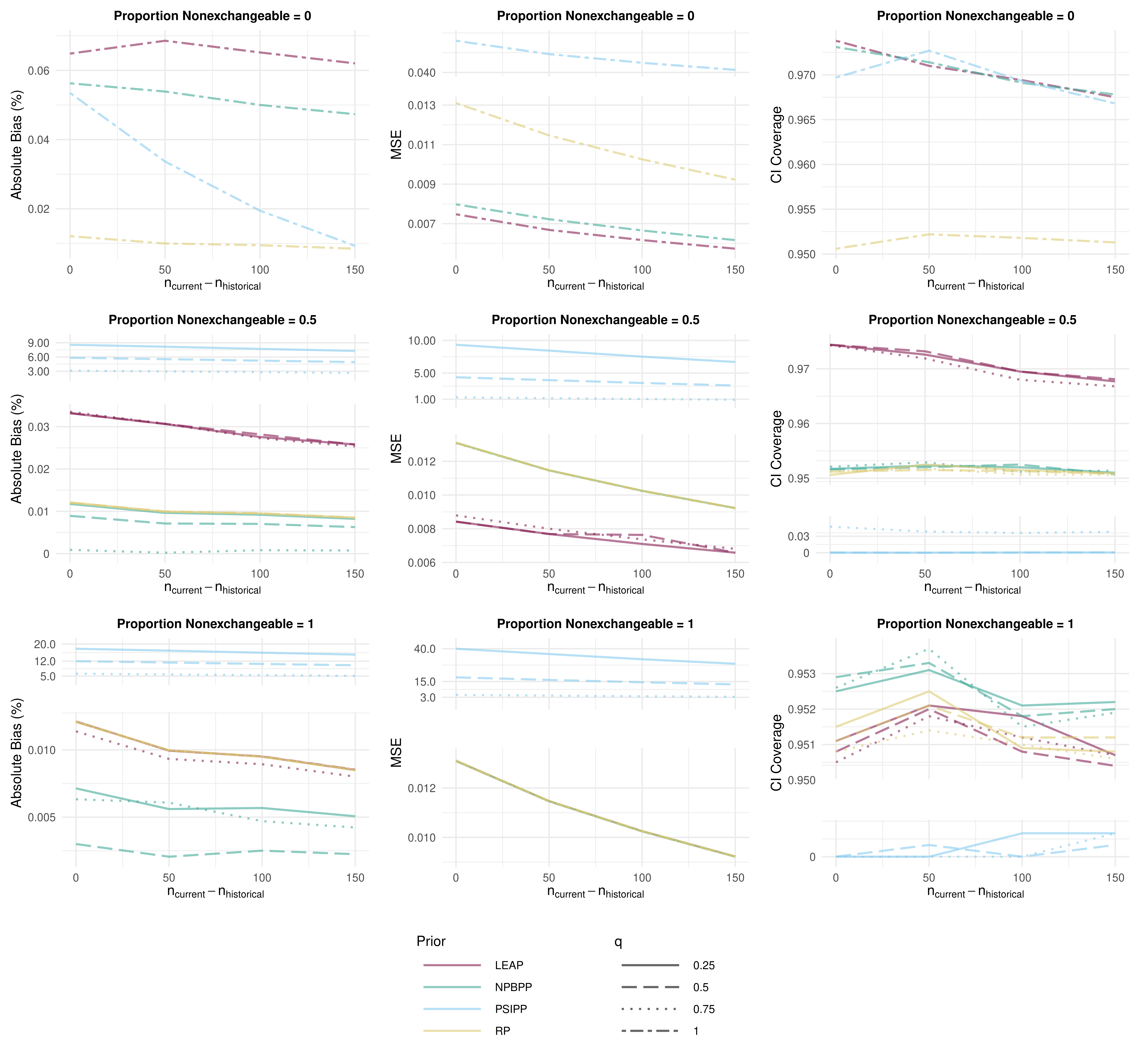
For the fully exchangeable setting (i.e., the first row), the LEAP has the highest PAB and the lowest MSE, which can be attributed to a bias-variance tradeoff. The bias between the priors, however, is negligible, as the maximum observed PAB for the LEAP is less than 0.08%. The LEAP and NPBPP have similar MSEs, while the MSE under the PSIPP is over $6$ times that of the LEAP. All three historical data priors had comparable CI coverage.

The PSIPP has poor performance under partial exchangeability and full unexchangeability, where it must be represented as a separate axis. The CI coverage is near 0 for all simulation scenarios and the bias is inflated up to 20%. This may be because the PSIPP is a static borrowing prior, where the amount of borrowing is taken to be fixed based on the PS (which is treated as known and fixed).

Under full unexchangeability (i.e., the third row), the LEAP and the NPBPP are again similar in terms of PAB, MSE, and CI coverage, where they essentially have the same features as a reference prior. Where they differ the most is under half exchangeability (i.e., the second row). We see that the LEAP has slightly inflated bias compared to the reference prior and the PBNPP, with an MSE that is about 33% less than the reference prior across the sample sizes. The LEAP also is the only prior to have higher than nominal CI coverage. This validates the conjecture in Section 3 that efficiency gains can be achieved even if only a fraction of individuals in the historical data are exchangeable.

Overall, it appears that the LEAP is the best performer among these three priors. Having CI coverage at the nominal level under a fully unexchangeable setting is similar to type I error control, which suggests that the LEAP may be a good option when borrowing from external controls. Only the LEAP exhibited efficiency gains under partial exchangeability whereas the performance of the information borrowing priors was similar under full exchangeability.

References

- Warasi et al. [2016] Md S. Warasi, Joshua M. Tebbs, Christopher S. McMahan, and Christopher R. Bilder. Estimating the prevalence of multiple diseases from two-stage hierarchical pooling. Statistics in Medicine, 35(21):3851–3864, 2016. ISSN 1097-0258. doi:10.1002/sim.6964. URL http://onlinelibrary.wiley.com/doi/abs/10.1002/sim.6964.
- Isakov and Kuriwaki [2020] Michael Isakov and Shiro Kuriwaki. Towards principled unskewing: Viewing 2020 election polls through a corrective lens from 2016. Harvard Data Science Review, 2(4):69, 2020.
- Lorencin and Pantoš [2017] Ivan Lorencin and Miloš Pantoš. Evaluating Generating Unit Unavailability Using Bayesian Power Priors. IEEE Transactions on Power Systems, 32(3):2315–2323, May 2017. ISSN 1558-0679. doi:10.1109/TPWRS.2016.2603469. Conference Name: IEEE Transactions on Power Systems.
- Louzada et al. [2021] Francisco Louzada, Diego Carvalho do Nascimento, and Osafu Augustine Egbon. Spatial Statistical Models: An Overview under the Bayesian Approach. Axioms, 10(4):307, December 2021. ISSN 2075-1680. doi:10.3390/axioms10040307. URL https://www.mdpi.com/2075-1680/10/4/307.
- Young and Chen [2022] Linda J. Young and Lu Chen. Using Small Area Estimation to Produce Official Statistics. Stats, 5(3):881–897, September 2022. ISSN 2571-905X. doi:10.3390/stats5030051. URL https://www.mdpi.com/2571-905X/5/3/51. Number: 3 Publisher: Multidisciplinary Digital Publishing Institute.
- König et al. [2021] Christoph König, Sarah Depaoli, Haiyan Liu, and Rens van de Schoot. Moving Beyond Non-informative Prior Distributions: Achieving the Full Potential of Bayesian Methods for Psychological Research. Frontiers in Psychology, 12:809719, December 2021. ISSN 1664-1078. doi:10.3389/fpsyg.2021.809719. URL https://www.ncbi.nlm.nih.gov/pmc/articles/PMC8695424/.
- Azzolina et al. [2021] Danila Azzolina, Giulia Lorenzoni, Silvia Bressan, Liviana Da Dalt, Ileana Baldi, and Dario Gregori. Handling Poor Accrual in Pediatric Trials: A Simulation Study Using a Bayesian Approach. International Journal of Environmental Research and Public Health, 18(4):2095, February 2021. ISSN 1661-7827. doi:10.3390/ijerph18042095. URL https://www.ncbi.nlm.nih.gov/pmc/articles/PMC7924849/.
- Chow and Huang [2020] Shein-Chung Chow and Zhipeng Huang. Innovative design and analysis for rare disease drug development. Journal of Biopharmaceutical Statistics, 30(3):537–549, May 2020. ISSN 1054-3406. doi:10.1080/10543406.2020.1726371. URL https://doi.org/10.1080/10543406.2020.1726371.
- Ibrahim and Chen [2000] Joseph G. Ibrahim and Ming-Hui Chen. Power prior distributions for regression models. Statistical Science, 15(1):46–60, February 2000. ISSN 0883-4237, 2168-8745. doi:10.1214/ss/1009212673. URL http://projecteuclid.org/euclid.ss/1009212673.
- Hobbs et al. [2012] Brian P. Hobbs, Daniel J. Sargent, and Bradley P. Carlin. Commensurate Priors for Incorporating Historical Information in Clinical Trials Using General and Generalized Linear Models. Bayesian Analysis, 7(3):639–674, August 2012. ISSN 1931-6690. doi:10.1214/12-BA722. URL https://www.ncbi.nlm.nih.gov/pmc/articles/PMC4007051/.
- Schmidli et al. [2014] Heinz Schmidli, Sandro Gsteiger, Satrajit Roychoudhury, Anthony O’Hagan, David Spiegelhalter, and Beat Neuenschwander. Robust meta-analytic-predictive priors in clinical trials with historical control information. Biometrics, 70(4):1023–1032, 2014. ISSN 1541-0420. doi:10.1111/biom.12242. URL http://onlinelibrary.wiley.com/doi/abs/10.1111/biom.12242.
- Papp et al. [2015] Kim Papp, Kristian Reich, Craig L. Leonardi, Leon Kircik, Sergio Chimenti, Richard G. B. Langley, ChiaChi Hu, Randall M. Stevens, Robert M. Day, Kenneth B. Gordon, Neil J. Korman, and Christopher E. M. Griffiths. Apremilast, an oral phosphodiesterase 4 (PDE4) inhibitor, in patients with moderate to severe plaque psoriasis: Results of a phase III, randomized, controlled trial (Efficacy and Safety Trial Evaluating the Effects of Apremilast in Psoriasis [ESTEEM] 1). Journal of the American Academy of Dermatology, 73(1):37–49, July 2015. ISSN 0190-9622. doi:10.1016/j.jaad.2015.03.049. URL https://www.sciencedirect.com/science/article/pii/S0190962215014942.
- Paul et al. [2015] C. Paul, J. Cather, M. Gooderham, Y. Poulin, U. Mrowietz, C. Ferrandiz, J. Crowley, C. Hu, R.m. Stevens, K. Shah, R.m. Day, G. Girolomoni, and A.b. Gottlieb. Efficacy and safety of apremilast, an oral phosphodiesterase 4 inhibitor, in patients with moderate-to-severe plaque psoriasis over 52 weeks: a phase III, randomized controlled trial (ESTEEM 2). British Journal of Dermatology, 173(6):1387–1399, 2015. ISSN 1365-2133. doi:10.1111/bjd.14164. URL http://onlinelibrary.wiley.com/doi/abs/10.1111/bjd.14164.
- Rousseau and Mengersen [2011] Judith Rousseau and Kerrie Mengersen. Asymptotic behaviour of the posterior distribution in overfitted mixture models. Journal of the Royal Statistical Society: Series B (Statistical Methodology), 73(5):689–710, 2011. ISSN 1467-9868. doi:10.1111/j.1467-9868.2011.00781.x. URL http://onlinelibrary.wiley.com/doi/abs/10.1111/j.1467-9868.2011.00781.x.
- Duan et al. [2006] Yuyan Duan, Keying Ye, and Eric P. Smith. Evaluating water quality using power priors to incorporate historical information. Environmetrics, 17(1):95–106, 2006. ISSN 1099-095X. doi:10.1002/env.752. URL https://onlinelibrary.wiley.com/doi/abs/10.1002/env.752.
- Lu et al. [2022] Nelson Lu, Chenguang Wang, Wei-Chen Chen, Heng Li, Changhong Song, Ram Tiwari, Yunling Xu, and Lilly Q. Yue. Propensity score-integrated power prior approach for augmenting the control arm of a randomized controlled trial by incorporating multiple external data sources. Journal of Biopharmaceutical Statistics, 32(1):158–169, 2022. ISSN 1054-3406.
- Zigler et al. [2013] Corwin M. Zigler, Krista Watts, Robert W. Yeh, Yun Wang, Brent A. Coull, and Francesca Dominici. Model Feedback in Bayesian Propensity Score Estimation. Biometrics, 69(1):263–273, 2013. ISSN 1541-0420. doi:10.1111/j.1541-0420.2012.01830.x. URL http://onlinelibrary.wiley.com/doi/abs/10.1111/j.1541-0420.2012.01830.x.
- Ibrahim et al. [2015a] Joseph G. Ibrahim, Ming-Hui Chen, Mani Lakshminarayanan, Guanghan F. Liu, and Joseph F. Heyse. Bayesian probability of success for clinical trials using historical data. Statistics in Medicine, 34(2):249–264, January 2015a. ISSN 02776715. doi:10.1002/sim.6339. URL http://doi.wiley.com/10.1002/sim.6339.
- Carpenter et al. [2017] Bob Carpenter, Andrew Gelman, Matthew D Hoffman, Daniel Lee, Ben Goodrich, Michael Betancourt, Marcus Brubaker, Jiqiang Guo, Peter Li, and Allen Riddell. Stan: A probabilistic programming language. Journal of Statistical Software, 76(1), 2017.
- Ibrahim et al. [2015b] Joseph G. Ibrahim, Ming-Hui Chen, Yeongjin Gwon, and Fang Chen. The power prior: theory and applications. Statistics in Medicine, 34(28):3724–3749, 2015b. ISSN 1097-0258. doi:10.1002/sim.6728. URL http://onlinelibrary.wiley.com/doi/abs/10.1002/sim.6728.
- Rosenbaum and Rubin [1984] Paul R. Rosenbaum and Donald B. Rubin. Reducing Bias in Observational Studies Using Subclassification on the Propensity Score. Journal of the American Statistical Association, 79(387):516–524, 1984. ISSN 0162-1459. doi:10.2307/2288398. URL http://www.jstor.org/stable/2288398.
- Wang and Chen [2022] Chenguang Wang and Wei-Chen Chen. psrwe: PS-Integrated Methods for Incorporating RWE in Clinical Studies. 2022. URL https://CRAN.R-project.org/package=psrwe.
- Spiegelhalter et al. [2002] David J. Spiegelhalter, Nicola G. Best, Bradley P. Carlin, and Angelika Van Der Linde. Bayesian measures of model complexity and fit. Journal of the Royal Statistical Society: Series B (Statistical Methodology), 64(4):583–639, 2002. ISSN 1467-9868. doi:10.1111/1467-9868.00353. URL https://onlinelibrary.wiley.com/doi/abs/10.1111/1467-9868.00353.