Vector Quantized Time Series Generation with a Bidirectional Prior Model
Daesoo Lee Sara Malacarne Erlend Aune
Norwegian University- of Science and Technology Telenor Research Norwegian University- of Science and Technology BI Norwegian Business School Abelee
Abstract
Time series generation (TSG) studies have mainly focused on the use of Generative Adversarial Networks (GANs) combined with recurrent neural network (RNN) variants. However, the fundamental limitations and challenges of training GANs still remain. In addition, the RNN-family typically has difficulties with temporal consistency between distant timesteps. Motivated by the successes in the image generation (IMG) domain, we propose TimeVQVAE, the first work, to our knowledge, that uses vector quantization (VQ) techniques to address the TSG problem. Moreover, the priors of the discrete latent spaces are learned with bidirectional transformer models that can better capture global temporal consistency. We also propose VQ modeling in a time-frequency domain, separated into low-frequency (LF) and high-frequency (HF). This allows us to retain important characteristics of the time series and, in turn, generate new synthetic signals that are of better quality, with sharper changes in modularity, than its competing TSG methods. Our experimental evaluation is conducted on all datasets from the UCR archive, using well-established metrics in the IMG literature, such as Fréchet inception distance and inception scores. Our implementation on GitHub: https://github.com/ML4ITS/TimeVQVAE.
1 INTRODUCTION
TSG models have been developed to overcome insufficient training data due, for example, to acquisition difficulties or strict privacy constraints (Li et al., 2015; Esteban et al., 2017; Yoon et al., 2019; Ni et al., 2020a; Smith and Smith, 2020; Li et al., 2022; Zha, 2022). Current mainstream TSG methods consist of combining RNNs with the GAN architecture, as done in RCGAN (Esteban et al., 2017), TimeGAN (Yoon et al., 2019), and SigCWGAN (Ni et al., 2020a). However, such methods are unable to effectively produce long sequences, given the limitation of the RNN model in keeping track of temporal dependencies between inputs that are distant in time (Vaswani et al., 2017). This problem is tackled by Li et al., 2022 with TTS-CGAN (Transformer Time-Series Conditional GAN), where the RNN model is replaced by a transformer model (Vaswani et al., 2017). The challenges of training GANs, such as non-convergence, mode collapse, generator-discriminator unbalance, and sensitive hyperparameter selection, however, still remain.
There has been much evidence in the IMG literature that VQ-based models and diffusion models significantly outperform the GAN alternatives (Yu et al., 2022; Gafni et al., 2022; Chang et al., 2022; Saharia et al., 2022; Ramesh et al., 2022). Therefore, a meaningful performance gain is to be expected by extending analogous methodologies in the time series domain. With our proposal, which we call TimeVQVAE, we adopt the two-stage modeling approach appearing in (Van Den Oord et al., 2017). More specifically, VQ-VAE is used for the first stage and MaskGIT (Chang et al., 2022) for the second. Although there are other advanced approaches for the first stage, such as VQ-GAN (Esser et al., 2021) and ViT-VQGAN (Yu et al., 2021), VQ-VAE has been selected as it has shown good performance in several areas, and, to our knowledge, it has never been explored in the TSG domain. The advanced VQ methods could be further investigated in future work. MaskGIT proposes to use a bidirectional transformer model for the prior learning unlike VQ-VAE, VQ-GAN, and ViT-VQGAN, where autoregressive models are used. It has experimentally been shown that the bidirectional transformer can capture global consistency better and accelerates the data generation process and achieves better-quality synthetic samples.
In our work, VQ-VAE acts on the time-frequency domain. We, furthermore, propose to separate the VQ modeling into LF and HF, respectively. The time-frequency domain provides richer information, results in better VQ modeling than in the time domain, and it allows disentangling HF components, such as spikes, from LF components, such as trends, more easily. Frequency separation is also motivated by the different predictability and compressibility of LF and HF components, as LF components are more predictable and compressible than HF components by nature. Thus, we let our model generate the LF component first and only subsequently the HF component, which could be viewed as defining the overall shape first and then filling in the details. Frequency separation also allows us to more precisely address several useful downstream tasks, such as anomaly detection for LF and HF components respectively, with explainable restoration (Marimont and Tarroni, 2021). Another related task is time series forecasting using discrete latent vectors, as explored in (Rasul et al., 2022), where an autoregressive model is trained in the discrete latent space, showing competitive forecasting performance. With the proposed LF-HF separation, the VQ forecasting problem can be further eased: LF components can be easily predicted while HF components can be quantified for uncertainty using the likelihood of individual tokens. In our proposed method, TimeVQVAE, we use STFT to transform the time series into the time-frequency domain and split it into LF and HF regions. Then, two sets of encoder, decoder, and vector-quantizer are used to learn the discrete latent spaces for LF and HF, respectively. Next, priors of the LF and HF discrete latent spaces are learned with two bidirectional transformer models. Lastly, we propose to jointly sample sets of LF and HF discrete latent vectors from the learned priors and decode them into time series with the learned decoders.
To evaluate generated samples fairly, robust evaluation metrics and diverse benchmark datasets are necessary. There has, however, been a lack of agreement for which evaluation metrics to use in the TSG literature (Brophy et al., 2021) and most TSG studies have been evaluated only on a small range of datasets (Esteban et al., 2017; Yoon et al., 2019; Ni et al., 2020a; Li et al., 2022; Zha, 2022; Desai et al., 2021). A common visual comparative evaluation of TSG is carried out using PCA and t-SNE on time series (Yoon et al., 2019; Desai et al., 2021; Zha, 2022; Li et al., 2022). But because this cannot be reported as a single value metric, its usability is limited. Also, because each element of time series does not carry semantically-meaningful information but time-step information, the principal axes found by PCA are not effective in capturing the realism of time series. There are other metrics that are occasionally used, such as the discriminative and predictive scores (Yoon et al., 2019; Desai et al., 2021; Zha, 2022), but there is no consensus for those yet, as they lack stability in the sense that the scores can be largely inconsistent for the same methods across different studies (Yoon et al., 2019; Desai et al., 2021; Zha, 2022). The IMG literature has already established standard metrics, such as the inception score (IS) (Salimans et al., 2016), Fréchet inception distance (FID) score (Heusel et al., 2017), and Classification Accuracy Score (CAS) (Ravuri and Vinyals, 2019). Note that CAS is the same as TSTR (Training on Synthetic data and Testing on Real data).
In this work, we propose to use the above-listed metrics – IS and FID in particular – to evaluate TSG models on a wide range of diverse datasets from the UCR archive (Dau et al., 2018) as an evaluation protocol for TSG models. IS and FID score have rarely been used in the TSG literature because there is no pretrained model for time series unlike in the computer vision domain (Paszke et al., 2019). Smith and Smith, 2020 was the first to evaluate a TSG model in terms of FID scores over the UCR archive datasets. They trained the Fully Convolutional Network (FCN) model (Wang et al., 2017) on every available UCR dataset and computed FID scores using the pretrained FCN models. Because the FCN model is one of the strongest baselines for time series classification and can effectively capture pattern features of time series (Wang et al., 2017), it is reasonable to use the representations from such a model to compute the FID scores. Unfortunately, though, the pretrained FCN models are not provided by Smith and Smith, 2020 on any open-source platform. We thus follow the same protocol as (Smith and Smith, 2020) and contribute by sharing code for the pretrained FCN models on GitHub along with templates for computing the IS and FID scores; available on https://github.com/danelee2601/supervised-FCN. It can be easily installed via pip.
Experiments are conducted for unconditional sampling and class-conditional sampling over the entire UCR archive. Our results clearly demonstrate how our proposed method outperforms the current competing TSG models, such as GMMN (Li et al., 2015), RCGAN, TimeGAN, SigCWGAN, and TSGAN, in terms of IS, FID, and CAS.
To summarize, our contributions consist of:
-
use of VQ for TSG,
-
VQ modeling in the time-frequency domain,
-
latent space separation into LF and HF,
-
joint sampling from the LF and HF latent spaces,
-
guided class-conditional sampling,
-
TSG evaluation on the entire UCR archive,
-
evaluation conducted by reporting IS, FID, and CAS,
-
releasing the pretrained FCN models on the UCR archive.
2 RELATED WORK
2.1 Time Series Generation
GMMN
employs maximum mean discrepancy (MMD). MMD is utilized to partially overcome the unstable training problem of GAN. GMMN has a simple objective that can be interpreted as matching all orders of statistics between real samples and synthetic samples. For TSG, GMMN can be combined with an RNN model. The MMD loss can be minimized between the generated time series by the RNN model and the real time series (Ni et al., 2020b).
RCGAN
sequentially generates time series using GAN: a latent vector from the noise space is sampled at every temporal step and an RNN model sequentially encodes them generating a synthetic time series.
TimeGAN
uses the conventional GAN training combined with a supervised learning approach. It aims to better preserve temporal dynamics of time series with the supervised learning loss.
SigCWGAN
addresses the problem of GANs struggling with capturing temporal dependencies by using the signature of a path (Kidger et al., 2019). Ni et al., 2020a proposes a Signature Wasserstein-1 (Sig-) metric that better captures temporal dependencies, and uses it as a discriminator. It provides a universal description of complex data streams without requiring expensive computation like the Wasserstein metric.
TTS-CGAN
uses a transformer model to overcome the distant temporal dependency problem appearing for the TSG RNN-based GAN models, such as RCGAN, TimeGAN, and SigCWGAN. It also proposes an approach to better induce the class-conditioning information into generated samples. Yet, the fundamental challenges in adopting GANs – that is, non-convergence, mode collapse, unbalance between generator and discriminator, sensitive hyperparameter selection – still exist (Arjovsky and Bottou, 2017; Salimans et al., 2016; Goodfellow, 2016; Goodfellow et al., 2020; Lucic et al., 2018).
TSGAN
is built using two WGANs (Arjovsky et al., 2017). The first WGAN generates a synthetic spectrogram from the noise latent vector, and the second WGAN receives the synthetic spectrogram and generates a time series. Therefore, there exist two discriminators. The first discriminator compares the spectrograms while the second discriminator compares the time series. Unlike RCGAN, TimeGAN, and SigCWGAN which use RNN-based generators, TSGAN’s generators use convolutional layers.
2.2 Vector Quantization-based Image Generation
VQ-VAE
is a type of variational autoencoder that uses vector quantization to obtain a discrete latent representation. There are two main differences between the classical VAE and the VQ-VAE: 1) VQ-VAE maps an input to a discrete latent space rather than a continuous space, and 2) instead of being static, the prior is learned. Because there is no constraint on the prior being Gaussian, as in VAE, VQ-VAE does not suffer from the posterior collapse. Moreover, the discretization allows for sharp and crisp synthetic images. For the sampling process, Van Den Oord et al., 2017 proposes the two-stage modeling approach: The first stage is for learning to project an input to the discrete latent space, that is, the so-called tokenization. To do that, an encoder, decoder, and codebook are trained. The codebook stores discrete codes (= discrete latent vectors/tokens). The second stage is for learning a prior of the discrete tokens in the discrete latent space. In VQ-VAE, PixelCNN (Van Den Oord et al., 2016) and WaveNet (Oord et al., 2016) are used as prior models for images and audio data, respectively.
MaskGIT
proposes a bidirectional transformer model for the prior learning instead of an autoregressive model as in VQ-VAE, VQ-GAN, and ViT-VQGAN. MaskGIT trains the prior model in the masked modeling manner. Chang et al., 2022 shows that using the bidirectional transformer model can accelerate the sampling process by 30-64 times and can achieve better quality and more diversity in the synthetic samples.
VQ-based Text-to-Image Generative Models
The current state-of-the-art (SOTA) IMG models include VQ and diffusion models, and not GANs. Among the SOTA VQ-based IMG models there are Parti (Yu et al., 2022), Make-A-Scene (Gafni et al., 2022), and DALLE-E (Ramesh et al., 2021). Their performances are quite competitive to their diffusion-based counterparts, such as Imagen (Saharia et al., 2022), DALL-E-2 (Ramesh et al., 2022), and GLIDE (Nichol et al., 2021). In light of such improvements in the image domain, a performance gain is to be expected also in the time series domain, if adopting one of the above-mentioned methodologies. With such motivation, our work explores the VQ-VAE approach for addressing the TSG problem.
3 METHOD
To produce good quality synthetic samples, optimization in stage 1 (tokenization) and stage 2 (prior learning) needs to be ensured. In the following subsections, our proposals for stages 1 and 2 are presented.

3.1 Stage 1: Learning Vector Quantization
In stage 1, an encoder, decoder, and codebook are to be optimized by effectively compressing the input into discrete tokens, while minimizing the information loss obtained by comparing the input with the output, given by decoding the selected tokens. In our work, VQ-VAE is used as a basis. VQ-VAE is known to produce sharper reconstructions (Van Den Oord et al., 2017) than AE and VAE (Bank et al., 2020; Pidhorskyi, 2019). However, we have experimentally found that a naive form of VQ-VAE still experiences difficulty with reconstructing time series, especially HF components. We tackle this problem by 1) augmenting the time series into the time-frequency domain, 2) separating the latent space modeling into LF and HF. By doing so, we can compress both LF and HF information of time series into the latent space better.
The overview of our proposal for stage 1 is presented in Fig. 1. The encoder and the decoder are denoted by and respectively. STFT and ISTFT stand for Short-time Fourier Transform and Inverse Short-time Fourier Transform, respectively. First, a time series is augmented into the time-frequency domain and separated into two branches where one is zero-padded on the HF region and the other is zero-padded on the LF region. Then, the encoders – and – project the time-frequency domains into the continuous latent space. has a higher downsampling rate than . The higher downsampling rate has a larger receptive field, therefore, enables to capture the overall structure of the data better, which results in globally-consistent synthetic samples (Esser et al., 2021). But such a high downsampling rate fails to retain the HF information in the embedding space (Rombach et al., 2022). To produce globally-consistent synthetic data with fine HF details, we use with a higher downsampling rate and with a lower downsampling rate. The continuous latent space is further transformed into the discrete latent space by the codebook via the argmin process. In the argmin process, each continuous token is compared to every discrete token in the codebook in terms of the Euclidean distance and replaced with the closest discrete token. That is the so-called quantization. Then, the decoders project the discrete latent spaces back into the time-frequency domains equipped with the corresponding zero-paddings, which are then mapped to the time domains via ISTFT. At the end, the two branches produce LF and HF components of the time series, respectively – and .
The codebook consists of discrete tokens , where each and denotes dimension size. The quantization process can be formulated as
| (1) |
where denotes the activation map after the encoder, in which and represent the height and width of the map, respectively. For each element in , denoted by , the corresponding continuous tokens are denoted by . The codebook-learning loss is then given by
| (2) |
where denotes the time series, denotes the stop-gradient operation, denotes the zero-padding operation on either the LF or HF region, denotes the discrete token for either LF or HF, and is a weighting parameter for the commitment loss terms. The back-propagation through the non-differentiable quantization is achieved simply by copying the gradients from the decoder to the encoder.
The VQ loss also contains the reconstruction loss. In our proposal, the reconstruction tasks are conducted in both the time and time-frequency domains, similar to (Défossez et al., 2022). Thus, the reconstruction loss is given by
| (3) |
where is equal to , is the reconstruction of , and are obtained by applying ISTFT to and respectively.
The total training objective for stage 1 becomes:
| (4) |
3.2 Stage 2: Prior Learning
In stage 2, the encoder, decoder, and codebook are frozen and a model is trained on the pre-trained discrete tokens to learn the prior. Inspired by MaskGIT, a bidirectional transformer is used as the prior model. However, the original form of MaskGIT cannot be applied, as there are two different modalities for the tokens, i.e., LF and HF. Our proposal suggests an approach to overcome this problem.
Prior Model Training
An input can now be represented in terms of the codebook-indices of the discrete tokens and is equivalent to a sequence where, recall, and denote height and width of . More precisely, each element of such sequence is given by
| (5) |
In the naive MaskGIT, the prior is modelled by , where is the masked sequence. During training, a random subset of is replaced by a special [MASK] token to produce . In our proposal, we model the prior11 1 Full derivation is available in Appendix A. by . The overview of the prior model training is presented in Fig. 2, where denotes the predicted . Two bidirectional transformers are used: one for and the other for ; is modelled by the LF bidirectional transformer and is modelled by the HF bidirectional transformer.

The training objective is to minimize the negative log-likelihood of the masked tokens, that is,
| (6) |
where and represent the parameters of the LF and HF bidirectional transformers, respectively.
Iterative Decoding
In theory, the prior model can predict all the [MASK] tokens and generate a synthetic sample in a single step. However, challenges are encountered if one proceeds this way. Thus, Chang et al., 2022 proposed to predict the [MASK] tokens in iterative multiple steps, i.e., iterative decoding. The overview of MaskGIT’s iterative decoding is presented in Fig. 3. The decoding process goes from to . To generate a synthetic sample, we start from a sequence that entirely consists of the [MASK] token indices, which we denote by . We then make predictions for all the [MASK] tokens , for and any . A number of with the largest probabilities are selected to form . This number is determined by a mask scheduling function. Additionally, Chang et al., 2022 used temperature annealing to encourage sample diversity. We use the cosine mask scheduling function and the temperature annealing following (Chang et al., 2022).

However, because we have two types of , that is, and , the decoding iteration requires two passes. The overview of the proposed double-pass iterative decoding is presented in Fig. 4, motivated by Jukebox’s ancestral sampling (Dhariwal et al., 2020). In the first pass, is decoded starting from . In the second pass, is decoded starting from , using the conditional probability dependent on computed in the first pass. The second pass mimics the training objective by by assuming and . To better ensure the assumption, the stochastic sampling (Lee et al., 2022) is used to stochastically sample and during training. It can reduce the discrepancy between predictions in training and inference. With the stochastic sampling, is sampled as where denotes the softmax distribution.

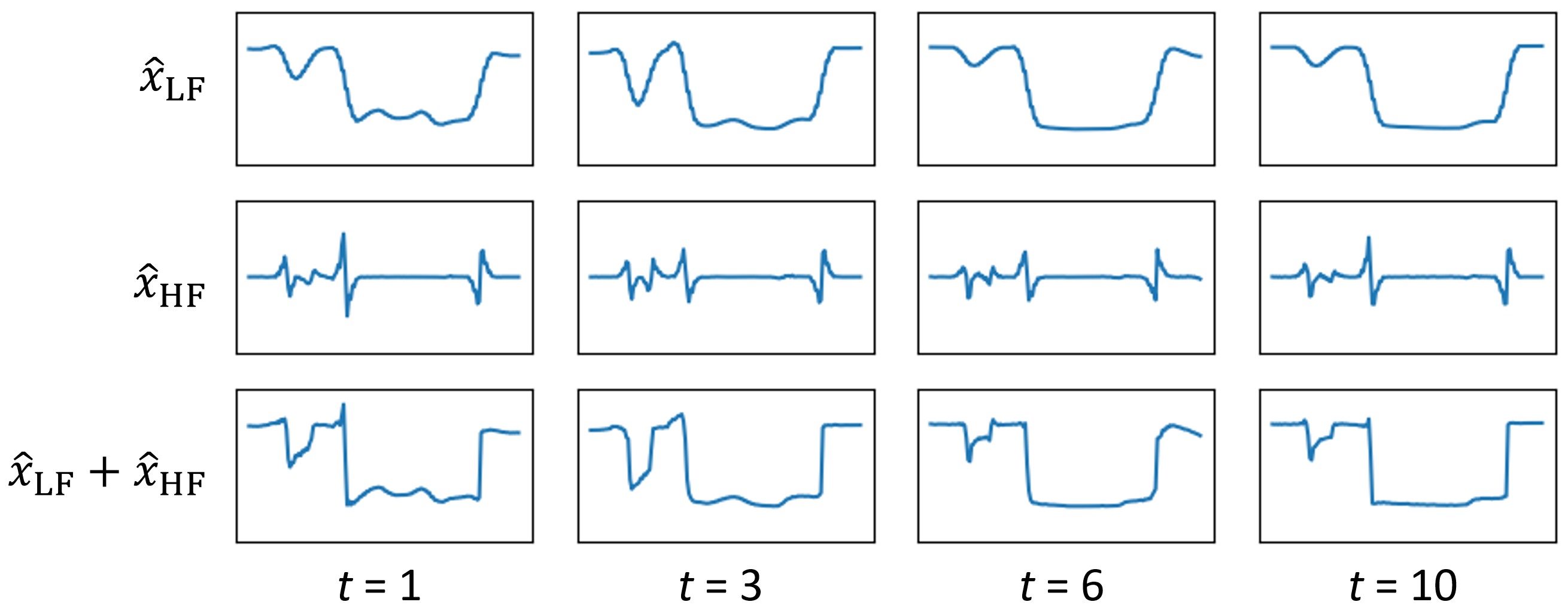
To generate synthetic time series, and are mapped back to their corresponding discrete tokens and . Afterwards, the discrete tokens are decoded to and , respectively. The complete synthetic time series is obtained by . An illustrative example of the proposed iterative decoding is presented in Fig. 5.
Learning to Sample both Unconditionally and Class-Conditionally
We train our model such that it can generate synthetic time series both unconditionally and class-conditionally. It is achieved by appending a class token index to similar to how a class token is appended in the Vision Transformer model (Dosovitskiy et al., 2020). Then is stochastically sampled by Ø where indicates no-class (for unconditional sampling) and indicates a certain class (for class-conditional sampling). This approach is adopted from the classifier-free guidance technique (Ho and Salimans, 2022). The probability of sampling is given by , so the probability of sampling one of the is given by . Following (Ho and Salimans, 2022), is set to 0.2. Gafni et al., 2022 proposes guided sampling for a VQ-based text-to-image model. We slightly modify it and propose guided class-conditional sampling: where is the guidance scale and the subscript denotes the guided class-conditional sampling. When is larger than 1, class-conditional sampling complies with class information better.
4 EXPERIMENTS22 2 Full results are available in Appendix E.
4.1 Evaluation Metrics
There are mainly three metrics used in the experiments: IS, FID score, and CAS. IS measures the quality of synthetic samples by using the entropy of the distribution of labels predicted by a pretrained model – i.e.,, Inception v3 (Szegedy et al., 2015) for IMG and FCN for TSG in this work – and evenness of the predictions across all labels. IS ranges from 1 to the number of classes. Better quality corresponds to higher IS. Unlike IS, FID score measures the quality by comparing distributions of generated samples and real samples. Its lowest score is 0 and it has no upper boundary. Better quality corresponds to lower FID. CAS is used to assess the quality of class-conditionally generated samples. It involves first training a classifier on synthetic samples – i.e., ResNet-50 (He et al., 2016) for IMG and FCN for TSG in this work – and then testing on real data, measuring the resulting accuracy.
4.2 Experimental Setup
All datasets from the UCR archive are used in the experiments. Each dataset is normalized such that it has zero mean and unit variance, following (Franceschi et al., 2019). For our encoder and decoder, those from VQ-VAE are adopted. Our implementation for VQ uses the library from (Wang et al., 2022). The implementation of the prior models, i.e., bidirectional transformers, is taken from (Wang, 2022). Further details on the parameter choices and implementation are available in Appendix C.
4.3 Unconditional Time Series Generation
GMMN, RCGAN, TimeGAN, SigCWGAN, and TimeVQVAE are compared for the unconditional sampling experiment in terms of FID and IS in Fig. 6. No code is available for TTS-CGAN at the time of writing, thus, it has not been included in the comparative study. The implementations of the competing models are taken from (Ni et al., 2020b). Among them, RCGAN and TimeGAN are the two most compared methods in the TSG literature. The model sizes are adjusted to be comparable to each other. Although TSGAN reports the FID scores on the UCR datasets, the reported FID scores are far off the normal range of the FID scores, that is, the scores are too high. Thus, due to the concern of a potential miscalculation, TSGAN’s reported FID scores are not used here. Fig. 6 shows that TimeVQVAE considerably outperforms its competing methods. Fig. 7 presents visualization of generated samples by the different methods. It is noticeable that the competing methods suffer from the limitation of RNN, that is, RNN typically has difficulties with temporal consistency between two distant timesteps. TimeVQVAE does not have the problem because all time steps are globally attended by the transformer’s self-attention mechanism.


4.4 Class-conditional Time Series Generation
Smith and Smith, 2020 reports CAS of WGAN and TSGAN on 70 subset datasets of the UCR archive. In Fig. 8, WGAN, TSGAN, and TimeVQVAE are compared for the class-conditional sampling in terms of CAS. , in this experiment, is set to 1. It indicates the synthetic sample distributions generated by TimeVQVAE is closer to the real distribution than WGAN and TSGAN. There is another advantage of TimeVQVAE. Smith and Smith, 2020 implements the class-conditional sampling by training the same model times on different subsets of a dataset according to different classes. TimeVQVAE, on the other hand, is trained for unconditional and class-conditional sampling at the same time.

4.5 Ablation Study
Naive VQ-VAE vs TimeVQVAE
Our proposed VQ modeling adds several novelties on top of VQ-VAE. Two cases are experimented: 1) naive VQ-VAE for stage 1 with the MaskGIT’s approach for stage 2, 2) TimeVQVAE. The naive VQ-VAE simply takes time series instead of images. Fig. 9 shows the considerable performance advantage of TimeVQVAE over its naive form.


VQ in Time and Time-frequency Domains
The VQ modeling can be done in the time domain – the naive VQ-VAE for stage 1 – or in the time-frequency domain as proposed. Fig. 10 shows that the VQ modeling in the time-frequency domain is more beneficial. To sorely compare the domain difference, the LF-HF separation is not used for the latter case and both cases have the same downsampling rate.


Separation of LF and HF Latent Spaces
The LF and HF latent spaces are separately learned in TimeVQVAE. Fig. 11 shows the positive effects of the LF-HF separation.


Guided Class-conditional Sampling
Fig. 12 shows that the higher results in the clearer class-boundaries of the generated samples.

Perceptual Loss
In VQ-GAN, the GAN and perceptual losses are additionally used from VQ-VAE. Those losses help generate perceptually-pleasing images. We experiment with the perceptual loss function proposed by Dosovitskiy and Brox, 2016, where denotes a pretrained model for feature extraction and and are real and reconstructed samples, respectively. In our experiments, the pretrained FCN model is used as . The effects of the perceptual loss are presented in Fig. 13. A minor yet positive performance gain is achieved, similarly to the IMG studies (Johnson et al., 2016).


5 LIMITATIONS
Because TimeVQVAE incorporates the Fourier Transform, it has difficulties with digital signal-like time series such as the Earthquakes and Computers datasets from the UCR archive. This problem, perhaps, could be overcome by employing the Wavelet Transform. It has the advantage of better locality in the time and frequency domains than STFT. Also, MaskGIT has some drawbacks (Lezama et al., 2022). Its token selection is made independently for each token and is based on predicted confidence by the generator, which can be prone to a modeling error. Moreover, the selected tokens are not correctable in a later iteration. Resolving the above-mentioned limitations could lead to better TSG.
6 CONCLUSION
Motivated by the successes in the IMG literature, we propose TimeVQVAE for TSG by leveraging VQ-VAE. Our experiments show that TimeVQVAE outperforms its competing methods in both unconditional and class-conditional sampling, plus it can be trained for both tasks at the same time, which greatly increases efficiency. Moreover, positive performance gains are shown by adopting VQ modeling in the time-frequency domain, carrying out LF-HF latent space separation, and including the guided class-conditional sampling and the perceptual loss.
Acknowledgements
We would like to thank the Norwegian Research Council for funding the Machine Learning for Irregular Time Series (ML4ITS) project (312062). This funding directly supported this research. We also would like to thank Prof. Eamonn Keogh and all the people who have contributed to the UCR time series classification archive for their selfless work.
References
- Arjovsky and Bottou, (2017) Arjovsky, M. and Bottou, L. (2017). Towards principled methods for training generative adversarial networks. arXiv preprint arXiv:1701.04862.
- Arjovsky et al., (2017) Arjovsky, M., Chintala, S., and Bottou, L. (2017). Wasserstein generative adversarial networks. In International conference on machine learning, pages 214–223. PMLR.
- Bank et al., (2020) Bank, D., Koenigstein, N., and Giryes, R. (2020). Autoencoders. arXiv preprint arXiv:2003.05991.
- Brophy et al., (2021) Brophy, E., Wang, Z., She, Q., and Ward, T. (2021). Generative adversarial networks in time series: A survey and taxonomy. arXiv preprint arXiv:2107.11098.
- Chang et al., (2022) Chang, H., Zhang, H., Jiang, L., Liu, C., and Freeman, W. T. (2022). Maskgit: Masked generative image transformer. In Proceedings of the IEEE/CVF Conference on Computer Vision and Pattern Recognition, pages 11315–11325.
- Dau et al., (2018) Dau, H. A., Keogh, E., Kamgar, K., Yeh, C.-C. M., Zhu, Y., Gharghabi, S., Ratanamahatana, C. A., Yanping, Hu, B., Begum, N., Bagnall, A., Mueen, A., Batista, G., and Hexagon-ML (2018). The ucr time series classification archive.
- Défossez et al., (2022) Défossez, A., Copet, J., Synnaeve, G., and Adi, Y. (2022). High fidelity neural audio compression. arXiv preprint arXiv:2210.13438.
- Deng et al., (2009) Deng, J., Dong, W., Socher, R., Li, L.-J., Li, K., and Fei-Fei, L. (2009). Imagenet: A large-scale hierarchical image database. In 2009 IEEE conference on computer vision and pattern recognition, pages 248–255. Ieee.
- Desai et al., (2021) Desai, A., Freeman, C., Wang, Z., and Beaver, I. (2021). Timevae: A variational auto-encoder for multivariate time series generation. arXiv preprint arXiv:2111.08095.
- Dhariwal et al., (2020) Dhariwal, P., Jun, H., Payne, C., Kim, J. W., Radford, A., and Sutskever, I. (2020). Jukebox: A generative model for music. arXiv preprint arXiv:2005.00341.
- dome272, (2022) dome272 (2022). dome272/MaskGIT-pytorch. https://github.com/dome272/MaskGIT-pytorch.
- Dosovitskiy et al., (2020) Dosovitskiy, A., Beyer, L., Kolesnikov, A., Weissenborn, D., Zhai, X., Unterthiner, T., Dehghani, M., Minderer, M., Heigold, G., Gelly, S., et al. (2020). An image is worth 16x16 words: Transformers for image recognition at scale. arXiv preprint arXiv:2010.11929.
- Dosovitskiy and Brox, (2016) Dosovitskiy, A. and Brox, T. (2016). Generating images with perceptual similarity metrics based on deep networks. Advances in neural information processing systems, 29.
- Esser et al., (2021) Esser, P., Rombach, R., and Ommer, B. (2021). Taming transformers for high-resolution image synthesis. In Proceedings of the IEEE/CVF conference on computer vision and pattern recognition, pages 12873–12883.
- Esteban et al., (2017) Esteban, C., Hyland, S. L., and Rätsch, G. (2017). Real-valued (medical) time series generation with recurrent conditional gans. arXiv preprint arXiv:1706.02633.
- Franceschi et al., (2019) Franceschi, J.-Y., Dieuleveut, A., and Jaggi, M. (2019). Unsupervised scalable representation learning for multivariate time series. Advances in neural information processing systems, 32.
- Gafni et al., (2022) Gafni, O., Polyak, A., Ashual, O., Sheynin, S., Parikh, D., and Taigman, Y. (2022). Make-a-scene: Scene-based text-to-image generation with human priors. arXiv preprint arXiv:2203.13131.
- Goodfellow, (2016) Goodfellow, I. (2016). Nips 2016 tutorial: Generative adversarial networks. arXiv preprint arXiv:1701.00160.
- Goodfellow et al., (2020) Goodfellow, I., Pouget-Abadie, J., Mirza, M., Xu, B., Warde-Farley, D., Ozair, S., Courville, A., and Bengio, Y. (2020). Generative adversarial networks. Communications of the ACM, 63(11):139–144.
- Hassani et al., (2021) Hassani, A., Walton, S., Shah, N., Abuduweili, A., Li, J., and Shi, H. (2021). Escaping the big data paradigm with compact transformers. arXiv preprint arXiv:2104.05704.
- He et al., (2016) He, K., Zhang, X., Ren, S., and Sun, J. (2016). Deep residual learning for image recognition. In Proceedings of the IEEE conference on computer vision and pattern recognition, pages 770–778.
- Heusel et al., (2017) Heusel, M., Ramsauer, H., Unterthiner, T., Nessler, B., and Hochreiter, S. (2017). Gans trained by a two time-scale update rule converge to a local nash equilibrium. Advances in neural information processing systems, 30.
- Ho and Salimans, (2022) Ho, J. and Salimans, T. (2022). Classifier-free diffusion guidance. arXiv preprint arXiv:2207.12598.
- Johnson et al., (2016) Johnson, J., Alahi, A., and Fei-Fei, L. (2016). Perceptual losses for real-time style transfer and super-resolution. In European conference on computer vision, pages 694–711. Springer.
- Kidger et al., (2019) Kidger, P., Bonnier, P., Perez Arribas, I., Salvi, C., and Lyons, T. (2019). Deep signature transforms. Advances in Neural Information Processing Systems, 32.
- Kingma and Ba, (2014) Kingma, D. P. and Ba, J. (2014). Adam: A method for stochastic optimization. arXiv preprint arXiv:1412.6980.
- Lee et al., (2022) Lee, D., Kim, C., Kim, S., Cho, M., and Han, W.-S. (2022). Autoregressive image generation using residual quantization. In Proceedings of the IEEE/CVF Conference on Computer Vision and Pattern Recognition, pages 11523–11532.
- Lezama et al., (2022) Lezama, J., Chang, H., Jiang, L., and Essa, I. (2022). Improved masked image generation with token-critic. arXiv preprint arXiv:2209.04439.
- Li et al., (2022) Li, X., Ngu, A. H. H., and Metsis, V. (2022). Tts-cgan: A transformer time-series conditional gan for biosignal data augmentation. arXiv preprint arXiv:2206.13676.
- Li et al., (2015) Li, Y., Swersky, K., and Zemel, R. (2015). Generative moment matching networks. In International conference on machine learning, pages 1718–1727. PMLR.
- Loshchilov and Hutter, (2017) Loshchilov, I. and Hutter, F. (2017). Decoupled weight decay regularization. arXiv preprint arXiv:1711.05101.
- Lucic et al., (2018) Lucic, M., Kurach, K., Michalski, M., Gelly, S., and Bousquet, O. (2018). Are gans created equal? a large-scale study. Advances in neural information processing systems, 31.
- Marimont and Tarroni, (2021) Marimont, S. N. and Tarroni, G. (2021). Anomaly detection through latent space restoration using vector quantized variational autoencoders. In 2021 IEEE 18th International Symposium on Biomedical Imaging (ISBI), pages 1764–1767. IEEE.
- nadavbh12 et al., (2021) nadavbh12, Huang, Y.-H., Huang, K., and Fernández, P. (2021). nadavbh12/VQ-VAE. https://github.com/nadavbh12/VQ-VAE.
- (35) Ni, H., Szpruch, L., Wiese, M., Liao, S., and Xiao, B. (2020a). Conditional sig-wasserstein gans for time series generation. arXiv preprint arXiv:2006.05421.
- (36) Ni, H., Szpruch, L., Wiese, M., Liao, S., and Xiao, B. (2020b). SigCGANs/Conditional-Sig-Wasserstein-GANs. https://github.com/SigCGANs/Conditional-Sig-Wasserstein-GANs.
- Nichol et al., (2021) Nichol, A., Dhariwal, P., Ramesh, A., Shyam, P., Mishkin, P., McGrew, B., Sutskever, I., and Chen, M. (2021). Glide: Towards photorealistic image generation and editing with text-guided diffusion models. arXiv preprint arXiv:2112.10741.
- Oord et al., (2016) Oord, A. v. d., Dieleman, S., Zen, H., Simonyan, K., Vinyals, O., Graves, A., Kalchbrenner, N., Senior, A., and Kavukcuoglu, K. (2016). Wavenet: A generative model for raw audio. arXiv preprint arXiv:1609.03499.
- Paszke et al., (2019) Paszke, A., Gross, S., Massa, F., Lerer, A., Bradbury, J., Chanan, G., Killeen, T., Lin, Z., Gimelshein, N., Antiga, L., Desmaison, A., Kopf, A., Yang, E., DeVito, Z., Raison, M., Tejani, A., Chilamkurthy, S., Steiner, B., Fang, L., Bai, J., and Chintala, S. (2019). Pytorch: An imperative style, high-performance deep learning library. In Wallach, H., Larochelle, H., Beygelzimer, A., d'Alché-Buc, F., Fox, E., and Garnett, R., editors, Advances in Neural Information Processing Systems 32, pages 8024–8035. Curran Associates, Inc. http://papers.neurips.cc/paper/9015-pytorch-an-imperative-style-high-performance-deep-learning-library.pdf.
- Pidhorskyi, (2019) Pidhorskyi, S. (2019). podgorskiy/VAE. GitHub. https://github.com/podgorskiy/VAE.
- Ramesh et al., (2022) Ramesh, A., Dhariwal, P., Nichol, A., Chu, C., and Chen, M. (2022). Hierarchical text-conditional image generation with clip latents. arXiv preprint arXiv:2204.06125.
- Ramesh et al., (2021) Ramesh, A., Pavlov, M., Goh, G., Gray, S., Voss, C., Radford, A., Chen, M., and Sutskever, I. (2021). Zero-shot text-to-image generation. In International Conference on Machine Learning, pages 8821–8831. PMLR.
- Rasul et al., (2022) Rasul, K., Park, Y.-J., Ramström, M. N., and Kim, K.-M. (2022). Vq-ar: Vector quantized autoregressive probabilistic time series forecasting. arXiv preprint arXiv:2205.15894.
- Ravuri and Vinyals, (2019) Ravuri, S. and Vinyals, O. (2019). Classification accuracy score for conditional generative models. Advances in neural information processing systems, 32.
- Rombach et al., (2022) Rombach, R., Blattmann, A., Lorenz, D., Esser, P., and Ommer, B. (2022). High-resolution image synthesis with latent diffusion models. In Proceedings of the IEEE/CVF Conference on Computer Vision and Pattern Recognition, pages 10684–10695.
- Saharia et al., (2022) Saharia, C., Chan, W., Saxena, S., Li, L., Whang, J., Denton, E., Ghasemipour, S. K. S., Ayan, B. K., Mahdavi, S. S., Lopes, R. G., et al. (2022). Photorealistic text-to-image diffusion models with deep language understanding. arXiv preprint arXiv:2205.11487.
- Salimans et al., (2016) Salimans, T., Goodfellow, I., Zaremba, W., Cheung, V., Radford, A., and Chen, X. (2016). Improved techniques for training gans. Advances in neural information processing systems, 29.
- Smith, (2020) Smith, K. E. (2020). One Dimensional Neural Time Series Generation. PhD thesis, Florida Institute of Technology.
- Smith and Smith, (2020) Smith, K. E. and Smith, A. O. (2020). Conditional gan for timeseries generation. arXiv preprint arXiv:2006.16477.
- Szegedy et al., (2015) Szegedy, C., Liu, W., Jia, Y., Sermanet, P., Reed, S., Anguelov, D., Erhan, D., Vanhoucke, V., and Rabinovich, A. (2015). Going deeper with convolutions. In Proceedings of the IEEE conference on computer vision and pattern recognition, pages 1–9.
- Tseng, (2021) Tseng, G. (2021). okrasolar/pytorch-timeseries. https://github.com/okrasolar/pytorch-timeseries.
- Van Den Oord et al., (2016) Van Den Oord, A., Kalchbrenner, N., and Kavukcuoglu, K. (2016). Pixel recurrent neural networks. In International conference on machine learning, pages 1747–1756. PMLR.
- Van Den Oord et al., (2017) Van Den Oord, A., Vinyals, O., et al. (2017). Neural discrete representation learning. Advances in neural information processing systems, 30.
- Vaswani et al., (2017) Vaswani, A., Shazeer, N., Parmar, N., Uszkoreit, J., Jones, L., Gomez, A. N., Kaiser, Ł., and Polosukhin, I. (2017). Attention is all you need. Advances in neural information processing systems, 30.
- Wang, (2022) Wang, P. (2022). lucidrains/x-transformers. https://github.com/lucidrains/x-transformers.
- Wang et al., (2022) Wang, P., Olsen, K., and Bouaziz, W. (2022). lucidrains/vector-quantize-pytorch. https://github.com/lucidrains/vector-quantize-pytorch.
- Wang et al., (2017) Wang, Z., Yan, W., and Oates, T. (2017). Time series classification from scratch with deep neural networks: A strong baseline. In 2017 International joint conference on neural networks (IJCNN), pages 1578–1585. IEEE.
- Yoon et al., (2019) Yoon, J., Jarrett, D., and Van der Schaar, M. (2019). Time-series generative adversarial networks. Advances in neural information processing systems, 32.
- Yu et al., (2021) Yu, J., Li, X., Koh, J. Y., Zhang, H., Pang, R., Qin, J., Ku, A., Xu, Y., Baldridge, J., and Wu, Y. (2021). Vector-quantized image modeling with improved vqgan. arXiv preprint arXiv:2110.04627.
- Yu et al., (2022) Yu, J., Xu, Y., Koh, J. Y., Luong, T., Baid, G., Wang, Z., Vasudevan, V., Ku, A., Yang, Y., Ayan, B. K., et al. (2022). Scaling autoregressive models for content-rich text-to-image generation. arXiv preprint arXiv:2206.10789.
- Zha, (2022) Zha, M. (2022). Time series generation with masked autoencoder. arXiv preprint arXiv:2201.07006.
- Zhang and Sennrich, (2019) Zhang, B. and Sennrich, R. (2019). Root mean square layer normalization. Advances in Neural Information Processing Systems, 32.
Appendix A FULL DERIVATION OF THE JOINT PROBABILITY OF AND
| (7) |
Recall that by HF and LF we mean high frequency and low frequency, respectively. In the above equation, is replaced by because is a subset of and information of the masked tokens is provided by . The equation can be further simplified with the following independence assumptions – and . The second and third terms of the last equation in Eq. (7) are simplified with the assumptions. We show the simplification of the second term and third term in order. Then, we finally show the simplified equation of Eq. (7).
The second term is simplified as:
| (8) |
The third term is simplified as:
| (9) |
Finally, Eq. (7) is simplified to:
| (10) |
Appendix B PRETRAINING SETUP FOR THE SUPERVISED FCN MODEL
The FCN model consists of a few convolutional blocks with the global average pooling (GAP), linear, and softmax layers followed. The source code for the FCN model is from (Tseng, 2021). Its representation (feature) vector for computing FID is extracted right after the GAP layer. AdamW (Loshchilov and Hutter, 2017) is used for an optimizer with {batch size: 256, initial learning rate (LR): 1e-3, LR scheduler: cosine scheduler, weight decay: 1e-5, max epoch: 1,000}. An open-source code for the pretrained FCN model is available on https://github.com/danelee2601/supervised-FCN.
Appendix C IMPLEMENTATION DETAILS
C.1 Datasets
For the unconditional and class-conditional sampling experiments, 128 datasets, i.e., all the datasets, from the UCR archive are used, on which IS, FID, and CAS are reported. CAS reported by Smith, 2020 is available only for 70 datasets out of 128. The missing scores are left blank in our result table below.
C.2 Evaluation Metrics: IS, FID, and CAS
To compute IS and FID, the same number of synthetic samples is unconditionally generated as that of a test set unless the test set has less than 256 samples. For datasets with less than 256 test samples, 256 synthetic samples are generated to better ensure the distribution of , which results in more consistent IS and FID score.
To compute CAS, the same number of synthetic samples per class is generated as that of a training set. If the training set has less than 1,000 samples, 1,000 samples are generated according to the class distribution of the training set to ensure the distribution of and to prevent the overfitting problem in the FCN model’s training. denotes the class token index. For instance, if a training set has 50 and 150 samples for class 1 and class 2, then 5 times the number of samples of each class are generated – that is, 250 for class 1 and 750 for class 2 – so that a total number of generated samples becomes 1,000. An average of 5 CAS from 5 runs is reported.
C.3 TimeVQVAE
STFT, ISTFT, and Convolutional Kernel and Stride Sizes
STFT and ISTFT are implemented with torch.stft and torch.istft, respectively. Their main parameter – n_fft, size of Fourier transform – can be any arbitrary integer, but we set it to 8 and we use default parameters for the rest. The frequency is separated into LF and HF by assigning the bottom rows (with the lowest ) to LF and the rest to HF. n_fft of 8 indicates that the frequency axis has a range of [1, 2, 3, 4, 5] and the length of the temporal dimension becomes half as long as a given time series because hop_length is set as n_fft/4 by default. This setting is chosen due to different temporal lengths of datasets, causing difficulties with selecting the convolutional kernel and stride sizes for downsampling. The encoder has several downsampling layers to compress an input into the latent space. The downsampling rate is determined by the kernel and stride sizes, typically downsampling by 2 with {kernel_size:4, stride=2, padding=1} at each downsampling layer. But a choice of the sizes is difficult because the temporal and frequency axes have different lengths across the different datasets. Therefore, we let the downsampling layers downsample along the temporal axis only, not the frequency axis. Then, the downsampling layer becomes nn.Conv2d with {kernel_size=(3,4), stride=(1,2), padding=(1,1)}. We have experimentally found that smaller n_fft such as 4 or 8 leads to better performance. That is associated with compression amount of input data. The higher n_fft leads to the wider frequency axis and shorter temporal axis, and the compression amount becomes smaller because the downsampling is only applied along the temporal axis. The global consistency of generated samples is typically poorer with the smaller compression amount (i.e., a lower downsampling rate).
Encoder and Decoder
The same encoder and decoder architectures from the VQ-VAE paper are used and their implementations are from (nadavbh12 et al., 2021). The encoder consists of downsampling convolutional blocks (Conv2d – BatchNorm2d – LeakyReLU), followed by residual blocks (LeakyReLU – Conv2d – BatchNorm2d – LeakyReLU – Conv2d). The downsampling convolutional layers are implemented by nn.Conv2d(kernel_size=(3,4), stride=(1,2), padding=(1,1)) – Note that the downsampling is to be conducted along the temporal axis only. The residual convolutional layers are implemented by nn.Conv2d(kernel_size=(3,3), stride=(1,1), padding=(1,1)). The decoder similarly has residual blocks, followed by upsampling convolutional blocks. The upsampling convolutional layers are implemented by nn.ConvTranspose2d(kernel_size=(3,4), stride=(1,2), padding=(1,1)). The downsampling rate is determined as . We set such that has width of around 8 and 32 for the LF and HF encoders and decoders, respectively. We refer to the width as the downsampled width. Note that the downsampled width cannot exactly be the specified value unless input length can be expressed as . We set the downsampling rate such that the width of can be as close as to the specified downsampled width. If a dataset has temporal length shorter than the downsampled width, the downsampling rate is set to 1 – i.e., no downsampling. Different sizes of the encoder and decoder are specified in Table 1. Large size is not considered due to our computational limitation. The Base-sized encoder and decoder are used for the unconditional and class-conditional sampling experiments.
| Sizes of the encoder & decoder | Small | Base |
|---|---|---|
| Hidden dimension size | 32 | 64 |
| Number of residual blocks | 2 | 4 |
Trick for Length Match Between and
When length of does not follow or is an odd number such as 89, length mismatch between and occurs. The problem can be easily resolved with the following trick: Adding one additional upsampling layer, followed by linear interpolation in the decoder. torch.nn.functional.interpolate(.., size=length(x), mode=’linear’) is used for the interpolation in our implementation. If the interpolation is only used without the additional upsampling layer, it leads to loss of high-frequency information in .
VQ
Our implementation for VQ-VAE is from (Wang et al., 2022). The codebook size is set to 32 and the code dimension size is the same as the hidden dimension size of the encoder and decoder for both LF and HF. Because the datasets from the UCR archive are less complex and much smaller than an image benchmark dataset such as ImagNet (Deng et al., 2009), the small-sized codebook was found to be sufficient. For the codebook-learning loss, we use both the commitment loss and the exponential moving average alternative, following (Wang et al., 2022). We use of 1. and the exponential moving average decay rate of 0.8. The codebook embeddings learned in stage 1 are used to initialize the codebook embeddings in stage 2 to benefit the prior learning. This can be especially helpful when a training set is very small such as Fungi. The dataset, Fungi, has only 18 training samples.
Prior Learning
The number of iterations, , is set to 10, following (Chang et al., 2022). Our implementation for MaskGIT is adopted from (dome272, 2022) and implementation for the prior models, i.e., bidirectional transformers, is from (Wang, 2022). Different sizes of the prior model are specified in Table 2. The Base size is used for the unconditional and class-conditional sampling experiments.To better stabilize the transformer model, we use Root Mean Square Layer Normalization proposed by Zhang and Sennrich, 2019.
| Size of the transformer | Small | Base |
|---|---|---|
| Hidden dimension size | 64 | 256 |
| Number of layers | 2 | 4 |
| Number of heads | 2 | 2 |
| Feed-forward ratio | 1 | 1 |
Optimizer
The AdamW optimizer is used with {batch size for stage 1: 128, batch size for stage 2: 256, initial LR: 1e-3, LR scheduler: cosine scheduler, weight decay: 1e-5}. Maximum epochs are {stage 1: 2,000, stage 2: 10,000} for the TimeVQVAE model in the unconditional and class-conditional sampling experiments.
C.4 GMMN, RCGAN, TimeGAN, and SigCWGAN
The implementations of GMMN, RCGAN, TimeGAN, and SigCWGAN from (Ni et al., 2020b) are used for the unconditional sampling experiments. For the above-mentioned methods, AR-FNN (Auto-Regressive Feed-forward Neural Network) proposed by Ni et al., 2020a is used for a generator and discriminator. To be comparable with TimeVQVAE in terms of a number of trainable parameters, the AR-FNN model is set to have 18 hidden layers and hidden dimension size of 32. The exact number of trainable parameters varies depending on datasets due to different lengths. The AR-FNN generator requires values at the previous timesteps to predict the next timesteps. is determined as 10% of input length. The longer compromises the integrity of data generation and the short makes the autoregressive model difficult to generate reasonable samples. is set to 1 for GMMN, RCGAN, and TimeGAN and 3 for SigCWGAN. does not have to be any larger because data is autoregressively generated at each timestep. The Adam optimizer (Kingma and Ba, 2014) is used for both generator and discriminator with {batch size: 256, initial LR: 2e-4 max_epochs: 10,000}.
C.5 Training the FCN Model for CAS
To compute CAS, the FCN model is trained on a set of synthetic samples. To train the FCN model, the AdamW optimizer is used with {batch size: 256, initial LR: 1e-3, LR scheduler: cosine scheduler, weight decay: 1e-5, max epochs: 1,000}. Basically, the same setting as the supervised FCN model is used.
Appendix D EXPERIMENT DETAILS FOR THE ABLATION STUDIES
The experiments for the ablation studies are conducted in a smaller scale due to a large number of experimental cases. The datasets with training set size equal or smaller than 1,000 are used – Yet, it still sums to 120 datasets; enough to capture the overall ranking. The optimizer settings are the same as in the prior section except that the maximum epochs of {stage 1: 1,000, stage 2: 5,000} are used. For the prior model, the Small-sized bidirectional model is used for all the ablation studies.
D.1 Model Details
There are 4 ablation studies with quantitative experiments. The model details for each ablation study are stated in the following paragraphs. Unless specified differently, the model parameters are the same as in the prior section.
Naive VQ-VAE vs TimeVQVAE
The Small-sized encoder and decoder are used for TimeVQVAE. TimeVQVAE has two sets of the encoder and decoder, but the naive VQ-VAE has one set of them. To be better comparable, size of the naive VQ-VAE’s encoder and decoder is set by {hidden dimension size: 32, number of residual blocks: 4} and is set to 64. The downsampled width of the naive VQ-VAE is to be around 8. For the naive VQ-VAE, 2-dimensional convolutional layers are replaced with the 1-dimensional convolutional layers as it takes 1-dimensional time series as an input instead of 2-dimensional time-frequency data.
VQ in Time and Time-frequency Domains
The encoder and decoder with {hidden dimension size: 32, number of residual blocks: 4} are used for both cases. Both, also, use the downsampled width of 8 and of 64. The case, VQ in Time domain, is identical to the naive VQ-VAE.
Separation of LF and HF Latent Spaces
The case without the LF-HF separation uses the encoder and decoder size of {hidden dimension size: 32, number of residual blocks: 4}, of 64, and the downsampled width of around 8. The case without the separation is identical to the case, VQ in Time-frequency domain, above. The case with the separation is identical to TimeVQVAE.
Perceptual Loss
TimeVQVAE with the Small-sized encoder and decoder is used.
Appendix E FULL RESULTS
The number of training parameters of TimeVQVAE in Tables 3-5 varies between 0.8 M and 1.6 M for stage 1 (i.e., encoder, codebook, and decoder) depending on the downsampled width, and the number varies between 2.3 M and 2.4 M for stage 2 (i.e., bidirectional transformer). The results for FID, IS, and CAS in Tables 3-5 are reported with mean and standard deviation of the scores over 3 runs.
| Dataset names | GMMN | RCGAN | TimeGAN | SigCWGAN | TimeVQVAE.mean | TimeVQVAE.std |
| ACSF1 | 74.3 | 98.3 | 81.3 | nan | 27.1 | 0.8 |
| Adiac | 98.2 | 54.3 | 45.1 | nan | 7.8 | 0.9 |
| AllGestureWiimoteX | 180.7 | nan | nan | nan | 3.8 | 0.7 |
| AllGestureWiimoteY | 23.5 | nan | nan | 660.4 | 3.0 | 0.5 |
| AllGestureWiimoteZ | nan | 2.8 | 7.9 | 278.9 | 1.8 | 0.2 |
| ArrowHead | 8.1 | 15.5 | 22.2 | nan | 2.0 | 0.3 |
| Beef | 215.2 | 36 | 18.3 | nan | 1.8 | 0.2 |
| BeetleFly | 246.4 | 348.5 | nan | nan | 2.1 | 1.2 |
| BirdChicken | 9.9 | 8.5 | 7.6 | 735.5 | 0.3 | 0.1 |
| BME | 77.6 | 179.6 | 140.1 | nan | 23.9 | 5.7 |
| Car | 101.5 | 579.5 | 186.1 | nan | 2.6 | 0.4 |
| CBF | 147.1 | 483.9 | 5.5 | 24.4 | 2.3 | 0.4 |
| Chinatown | 27.3 | 70.4 | 59.9 | 25.8 | 5.5 | 0.9 |
| ChlorineConcentration | 41.6 | 7.4 | 7.1 | 132.4 | 1.1 | 0.1 |
| CinCECGTorso | nan | 172.3 | 57 | nan | 7.7 | 1.5 |
| Coffee | 16.2 | 18.1 | nan | nan | 0.3 | 0.2 |
| Computers | 29.1 | nan | nan | 19.8 | 3.5 | 0.4 |
| CricketX | 115.8 | 404.8 | 23 | 26.9 | 3.0 | 0.5 |
| CricketY | 33 | nan | nan | 17.6 | 3.0 | 0.4 |
| CricketZ | 60.1 | 105.3 | 14.4 | 19.8 | 4.0 | 0.3 |
| Crop | 80.7 | 14.9 | 18.7 | 35.3 | 3.9 | 0.7 |
| DiatomSizeReduction | 138.6 | 232.9 | 88.7 | nan | 12.8 | 1.4 |
| DistalPhalanxOutlineAgeGroup | 13.9 | 9 | 110.6 | nan | 6.3 | 1.0 |
| DistalPhalanxOutlineCorrect | 9.2 | 12 | 16 | 50.4 | 1.8 | 0.3 |
| DistalPhalanxTW | 16.8 | 19.2 | 21.3 | nan | 13.2 | 1.5 |
| DodgerLoopDay | 56.8 | 429.9 | 30.1 | 14.4 | 1.9 | 0.2 |
| DodgerLoopGame | 44.8 | nan | 21.6 | 63.4 | 5.9 | 0.9 |
| DodgerLoopWeekend | 9.6 | 273.2 | 16.1 | 14.7 | 6.2 | 1.1 |
| Earthquakes | nan | nan | nan | 5.4 | 1.6 | 0.5 |
| ECG200 | 3 | 2.8 | 2.7 | 20.6 | 1.9 | 0.3 |
| ECG5000 | 26.6 | 4.5 | 35.2 | 55.9 | 0.7 | 0.0 |
| ECGFiveDays | 15 | 22.3 | 7.1 | 523.2 | 0.6 | 0.2 |
| ElectricDevices | 37.1 | 151.9 | 79.9 | 105.5 | 6.8 | 1.1 |
| EOGHorizontalSignal | 287.8 | 47.3 | 95.5 | nan | 3.5 | 0.6 |
| EOGVerticalSignal | 238.1 | 457.7 | 100.6 | nan | 6.8 | 1.2 |
| EthanolLevel | 19.4 | 15.7 | 18 | nan | 0.2 | 0.2 |
| FaceAll | 42.4 | 10.3 | nan | 33 | 4.4 | 0.0 |
| FaceFour | 18.6 | 65 | 56.5 | 26.5 | 3.6 | 1.3 |
| FacesUCR | 39.7 | 7.3 | 20.6 | 39.7 | 3.2 | 0.4 |
| FiftyWords | nan | 27.7 | 81.7 | 821.9 | 9.7 | 1.5 |
| Fish | nan | 36.3 | 47.4 | nan | 11.5 | 0.1 |
| FordA | 3.6 | 178 | nan | nan | 3.0 | 0.4 |
| FordB | nan | 45.6 | nan | nan | 1.4 | 0.6 |
| FreezerRegularTrain | 56 | 41.6 | 27.6 | 176.9 | 7.3 | 1.3 |
| FreezerSmallTrain | 49.3 | 32 | 42.7 | 109.6 | 9.5 | 0.7 |
| Fungi | 48.4 | 86 | 82.9 | nan | 2.1 | 0.5 |
| GestureMidAirD1 | nan | nan | nan | nan | 9.9 | 5.1 |
| GestureMidAirD2 | nan | nan | 306.8 | nan | 3.8 | 0.5 |
| GestureMidAirD3 | 214.7 | nan | nan | nan | 46.4 | 19.1 |
| GesturePebbleZ1 | 163.4 | 29.5 | 10.6 | 26.2 | 3.0 | 2.3 |
| GesturePebbleZ2 | 16.7 | 350.8 | 22.3 | 49.9 | 3.7 | 1.1 |
| GunPoint | 16 | 8.8 | 3.5 | nan | 0.8 | 0.4 |
| GunPointAgeSpan | 314.7 | 19.7 | 267.3 | nan | 1.1 | 0.5 |
| GunPointMaleVersusFemale | nan | 44.6 | 237.5 | 215.4 | 0.6 | 0.3 |
| GunPointOldVersusYoung | 14.1 | nan | 13.2 | nan | 0.3 | 0.1 |
| Ham | nan | 43.5 | 27.4 | 427 | 0.6 | 0.2 |
| HandOutlines | 9.4 | 3.7 | 1.3 | nan | 0.1 | 0.0 |
| Haptics | nan | nan | nan | nan | 2.5 | 0.2 |
| Herring | 35 | 3.9 | 75.8 | nan | 0.5 | 0.1 |
| HouseTwenty | 26.6 | nan | 38 | 100.3 | 4.8 | 2.7 |
| InlineSkate | 96 | 143.3 | 119.5 | nan | 13.3 | 5.0 |
| InsectEPGRegularTrain | 7.3 | 28.5 | 0.9 | 0.3 | 2.5 | 1.0 |
| InsectEPGSmallTrain | 121.2 | 113.5 | 125.9 | 80.8 | 3.6 | 3.3 |
| InsectWingbeatSound | 14.5 | 6.2 | 132.3 | nan | 9.9 | 0.7 |
| ItalyPowerDemand | 5.7 | 57.5 | 5.8 | 4.6 | 1.6 | 0.4 |
| LargeKitchenAppliances | 8.3 | 47.3 | 31.8 | 281 | 0.9 | 0.3 |
| Lightning2 | 19.5 | 8.6 | 71.7 | 162.3 | 1.2 | 0.4 |
| Lightning7 | 79.2 | 78.6 | 27 | 92.1 | 1.1 | 0.2 |
| Mallat | nan | 11.4 | nan | nan | 1.1 | 0.2 |
| Meat | 134.7 | 18.2 | nan | nan | 7.7 | 3.8 |
| MedicalImages | 20.9 | 24 | nan | 55.3 | 3.5 | 0.4 |
| MelbournePedestrian | 66.6 | 35.5 | 62.5 | 90.1 | 2.4 | 0.9 |
| MiddlePhalanxOutlineAgeGroup | 18.7 | 12.6 | 13.8 | 590.2 | 20.0 | 1.6 |
| MiddlePhalanxOutlineCorrect | 7.2 | 21.2 | 162.3 | 535.4 | 1.2 | 0.4 |
| MiddlePhalanxTW | 62.2 | 27.4 | 19.8 | nan | 3.3 | 0.5 |
| MixedShapesRegularTrain | 379 | 412.2 | nan | nan | 34.1 | 6.5 |
| MixedShapesSmallTrain | 20.6 | 13.3 | 262.1 | nan | 7.6 | 1.8 |
| MoteStrain | 5.6 | 5.9 | 4 | 13.9 | 1.5 | 0.3 |
| NonInvasiveFetalECGThorax1 | 438.5 | nan | nan | nan | 16.0 | 2.8 |
| NonInvasiveFetalECGThorax2 | 126.8 | 117.9 | 150 | nan | 30.6 | 13.9 |
| OliveOil | 9.8 | 9.5 | 9.9 | nan | 1.7 | 0.1 |
| OSULeaf | nan | nan | nan | nan | 13.2 | 0.9 |
| PhalangesOutlinesCorrect | 1.9 | 3 | 2.3 | 73.4 | 0.7 | 0.1 |
| Phoneme | nan | nan | nan | nan | 12.1 | 0.4 |
| PickupGestureWiimoteZ | 275.6 | 380.9 | nan | 116 | 2.1 | 0.2 |
| PigAirwayPressure | 111.2 | 188.5 | 642.6 | 274.4 | 38.1 | 11.9 |
| PigArtPressure | 291.4 | nan | nan | 80.3 | 72.4 | 13.3 |
| PigCVP | 107.6 | nan | nan | 343.3 | 57.7 | 9.7 |
| PLAID | 797.4 | nan | 335.9 | nan | 552.8 | 474.5 |
| Plane | 39.2 | 38.9 | 36.2 | nan | 6.6 | 0.5 |
| PowerCons | 18.3 | 15 | 16.5 | 30 | 1.0 | 0.4 |
| ProximalPhalanxOutlineAgeGroup | 73.2 | 93.9 | 22.1 | nan | 0.4 | 0.2 |
| ProximalPhalanxOutlineCorrect | 3.7 | 1.7 | 13.8 | nan | 0.4 | 0.2 |
| ProximalPhalanxTW | 60.8 | 24.2 | 16.2 | nan | 2.8 | 0.4 |
| RefrigerationDevices | nan | nan | nan | 9.2 | 16.2 | 3.6 |
| Rock | nan | nan | nan | 23.5 | 6.0 | 3.1 |
| ScreenType | 32.7 | nan | 30.9 | 28.4 | 6.3 | 0.8 |
| SemgHandGenderCh2 | 14.4 | nan | nan | 69.9 | 4.6 | 0.2 |
| SemgHandMovementCh2 | 164.6 | 71.8 | 199.1 | 59.4 | 14.1 | 0.3 |
| SemgHandSubjectCh2 | 37 | nan | nan | 108.1 | 29.6 | 2.3 |
| ShakeGestureWiimoteZ | nan | 42.5 | 22.4 | 116.7 | 2.4 | 0.7 |
| ShapeletSim | 8.4 | 2.6 | nan | 0.8 | 9.0 | 2.5 |
| ShapesAll | nan | nan | nan | nan | 14.4 | 2.2 |
| SmallKitchenAppliances | 19 | nan | 20.8 | 233.1 | 4.7 | 0.4 |
| SmoothSubspace | nan | 7.7 | 14.1 | 8.2 | 0.6 | 0.1 |
| SonyAIBORobotSurface1 | 31.7 | nan | 14.3 | 81.7 | 8.8 | 1.8 |
| SonyAIBORobotSurface2 | 22.6 | 21.2 | 14.5 | 10.7 | 1.4 | 0.3 |
| StarLightCurves | 27.6 | 42.9 | 6.7 | nan | 0.7 | 0.1 |
| Strawberry | 70.6 | 20.8 | 333.9 | nan | 0.4 | 0.1 |
| SwedishLeaf | 46.3 | 16.5 | 24.7 | 151.5 | 7.9 | 0.4 |
| Symbols | 33.8 | 29.9 | 57.2 | 407.6 | 5.6 | 1.6 |
| SyntheticControl | 14.7 | 12.6 | 14 | 17.4 | 3.7 | 0.9 |
| ToeSegmentation1 | 19.2 | 502.3 | nan | 7 | 4.1 | 0.6 |
| ToeSegmentation2 | 3.5 | 2.8 | 154.7 | 89 | 6.2 | 0.3 |
| Trace | 93 | 90.8 | 21.7 | 187.4 | 5.7 | 0.7 |
| TwoLeadECG | 10.4 | 12.2 | 8.7 | 49.5 | 0.2 | 0.1 |
| TwoPatterns | 15.4 | 31.8 | 29.6 | 51.3 | 2.2 | 0.6 |
| UMD | 454.1 | 11.4 | 15.5 | 501.3 | 1.2 | 0.4 |
| UWaveGestureLibraryAll | 737.2 | nan | nan | 586.1 | 4.5 | 0.2 |
| UWaveGestureLibraryX | 31.5 | nan | nan | nan | 6.8 | 0.3 |
| UWaveGestureLibraryY | nan | 22 | nan | nan | 7.0 | 0.0 |
| UWaveGestureLibraryZ | 9.6 | 24.3 | nan | nan | 27.7 | 2.5 |
| Wafer | 26.8 | nan | 23.6 | 164 | 1.5 | 0.3 |
| Wine | nan | nan | nan | nan | 0.4 | 0.1 |
| WordSynonyms | 34.4 | 11.3 | 42.3 | nan | 2.9 | 0.1 |
| Worms | nan | nan | nan | nan | 8.0 | 0.5 |
| WormsTwoClass | nan | nan | nan | nan | 8.0 | 1.5 |
| Yoga | nan | nan | nan | nan | 2.3 | 0.2 |
| Dataset names | GMMN | RCGAN | TimeGAN | SigCWGAN | TimeVQVAE.mean | TimeVQVAE.std |
| ACSF1 | 1.4 | 1.9 | 1.5 | 2 | 3.3 | 0.1 |
| Adiac | 1.1 | 1.4 | 1.6 | 1.6 | 6.2 | 0.3 |
| AllGestureWiimoteX | 3.6 | 3.2 | 4.3 | 1.5 | 2.5 | 0.2 |
| AllGestureWiimoteY | 3.4 | 3.2 | 3.1 | 1.7 | 3.0 | 0.1 |
| AllGestureWiimoteZ | 2.6 | 2.3 | 2.3 | 1 | 2.6 | 0.0 |
| ArrowHead | 1.9 | 1.1 | 1.1 | 1 | 2.5 | 0.1 |
| Beef | 1.2 | 1.4 | 1.5 | 1 | 2.7 | 0.2 |
| BeetleFly | 1 | 1.1 | 1 | 1 | 1.7 | 0.2 |
| BirdChicken | 1 | 1.1 | 1.1 | 1 | 1.8 | 0.0 |
| BME | 1 | 1.2 | 1.2 | 1.1 | 2.1 | 0.2 |
| Car | 1.7 | 1 | 1 | 1 | 2.3 | 0.1 |
| CBF | 1 | 1.1 | 1.5 | 1.1 | 2.7 | 0.0 |
| Chinatown | 1.8 | 1 | 1.3 | 1.6 | 2.0 | 0.0 |
| ChlorineConcentration | 1.2 | 2 | 1.9 | 1 | 1.6 | 0.1 |
| CinCECGTorso | 1.5 | 1.3 | 1.6 | 1 | 1.8 | 0.2 |
| Coffee | 1.1 | 1 | 1 | 1 | 1.9 | 0.0 |
| Computers | 1.2 | 1.8 | 1.4 | 1.2 | 1.6 | 0.1 |
| CricketX | 1.8 | 2 | 2.3 | 1.8 | 3.3 | 0.3 |
| CricketY | 2.3 | 3 | 3.6 | 2 | 3.6 | 0.1 |
| CricketZ | 3 | 1.9 | 2.5 | 1.9 | 3.3 | 0.1 |
| Crop | 5.7 | 7.7 | 7.8 | 7.5 | 17.0 | 0.1 |
| DiatomSizeReduction | 1 | 1.2 | 1.3 | 1 | 2.8 | 0.0 |
| DistalPhalanxOutlineAgeGroup | 1.5 | 1.6 | 1.3 | 1 | 1.9 | 0.1 |
| DistalPhalanxOutlineCorrect | 1.2 | 1.4 | 1.7 | 1.8 | 1.5 | 0.0 |
| DistalPhalanxTW | 1.9 | 1.9 | 1.7 | 2.1 | 2.5 | 0.2 |
| DodgerLoopDay | 1 | 1.2 | 1.2 | 1.3 | 2.6 | 0.2 |
| DodgerLoopGame | 1 | 1.2 | 1 | 1.1 | 1.9 | 0.0 |
| DodgerLoopWeekend | 1.2 | 1 | 1.6 | 1.1 | 1.9 | 0.0 |
| Earthquakes | 1.2 | 1 | 1 | 1.1 | 1.1 | 0.0 |
| ECG200 | 1.4 | 1.5 | 1.4 | 1.5 | 1.5 | 0.0 |
| ECG5000 | 1.7 | 1.7 | 1.6 | 1.6 | 2.0 | 0.0 |
| ECGFiveDays | 1.1 | 1 | 1.2 | 1.7 | 1.7 | 0.1 |
| ElectricDevices | 2.9 | 3.8 | 4.4 | 2.8 | 4.7 | 0.1 |
| EOGHorizontalSignal | 1.3 | 2.5 | 1.3 | 2 | 4.7 | 0.2 |
| EOGVerticalSignal | 1.5 | 1.7 | 1.7 | 1.2 | 3.2 | 0.1 |
| EthanolLevel | 1 | 1.1 | 1 | 2 | 1.3 | 0.1 |
| FaceAll | 2 | 2.2 | 3 | 1.8 | 5.3 | 0.2 |
| FaceFour | 1.2 | 1.3 | 1.1 | 1.2 | 2.7 | 0.2 |
| FacesUCR | 1 | 1.9 | 2.1 | 1.5 | 3.3 | 0.3 |
| FiftyWords | 2.7 | 1.9 | 1.3 | 1.8 | 4.6 | 0.2 |
| Fish | 1 | 1.2 | 1.2 | 1 | 3.1 | 0.0 |
| FordA | 1.5 | 1.3 | 1 | 1 | 1.5 | 0.0 |
| FordB | 1 | 1.7 | 1 | 1 | 1.4 | 0.1 |
| FreezerRegularTrain | 1 | 1 | 1 | 1.6 | 1.4 | 0.1 |
| FreezerSmallTrain | 1.8 | 2 | 1.9 | 1.2 | 1.9 | 0.0 |
| Fungi | 1 | 1.1 | 1.3 | 1 | 7.3 | 0.8 |
| GestureMidAirD1 | 2.1 | 2.5 | 2.6 | 1.4 | 3.4 | 0.5 |
| GestureMidAirD2 | 1.1 | 1.1 | 1.5 | 1 | 4.6 | 0.2 |
| GestureMidAirD3 | 3.3 | 2.9 | 1.7 | 2.6 | 2.0 | 0.1 |
| GesturePebbleZ1 | 1.2 | 1.1 | 2 | 1.4 | 2.9 | 0.5 |
| GesturePebbleZ2 | 1.3 | 1.7 | 1.9 | 1 | 2.8 | 0.2 |
| GunPoint | 1.4 | 1.3 | 1.6 | 1 | 1.9 | 0.0 |
| GunPointAgeSpan | 1.5 | 1.1 | 1 | 1 | 1.7 | 0.1 |
| GunPointMaleVersusFemale | 1 | 1.1 | 1 | 1 | 1.9 | 0.0 |
| GunPointOldVersusYoung | 1.7 | 1.3 | 1.9 | 1.3 | 1.9 | 0.0 |
| Ham | 1.1 | 1.5 | 1.4 | 1.3 | 1.6 | 0.1 |
| HandOutlines | 1.2 | 1 | 1.4 | 1 | 1.2 | 0.0 |
| Haptics | 1.9 | 1 | 1 | 1 | 1.9 | 0.0 |
| Herring | 1 | 1 | 1.1 | 1 | 1.3 | 0.0 |
| HouseTwenty | 1 | 1.2 | 1 | 1 | 1.6 | 0.0 |
| InlineSkate | 1.7 | 1.2 | 1.7 | 1 | 1.5 | 0.0 |
| InsectEPGRegularTrain | 2.5 | 2.2 | 2.8 | 2.8 | 2.5 | 0.2 |
| InsectEPGSmallTrain | 1 | 1 | 1 | 1 | 2.4 | 0.2 |
| InsectWingbeatSound | 2.3 | 1.8 | 1.1 | 1.5 | 2.9 | 0.1 |
| ItalyPowerDemand | 1.6 | 1.2 | 1.6 | 1.6 | 2.0 | 0.0 |
| LargeKitchenAppliances | 1.4 | 1.5 | 1.4 | 1.8 | 2.3 | 0.0 |
| Lightning2 | 1.2 | 1.2 | 1.5 | 1 | 1.6 | 0.0 |
| Lightning7 | 1 | 1.1 | 1.6 | 1.4 | 3.4 | 0.2 |
| Mallat | 1 | 1.1 | 1 | 1 | 4.6 | 0.5 |
| Meat | 1.1 | 1.2 | 1.4 | 1 | 1.2 | 0.2 |
| MedicalImages | 2.4 | 1.2 | 1.4 | 2.4 | 2.6 | 0.2 |
| MelbournePedestrian | 4.2 | 4.8 | 3.8 | 4.7 | 8.9 | 0.1 |
| MiddlePhalanxOutlineAgeGroup | 1.6 | 1.6 | 1.7 | 1.1 | 2.0 | 0.1 |
| MiddlePhalanxOutlineCorrect | 1.4 | 1.7 | 1.1 | 1.1 | 1.6 | 0.1 |
| MiddlePhalanxTW | 2.2 | 2 | 2.3 | 2.4 | 2.8 | 0.1 |
| MixedShapesRegularTrain | 2.2 | 1.9 | 2.3 | 1.2 | 1.3 | 0.1 |
| MixedShapesSmallTrain | 1.3 | 2.2 | 1.5 | 1 | 2.2 | 0.2 |
| MoteStrain | 1.8 | 1.5 | 1.4 | 1.2 | 1.9 | 0.0 |
| NonInvasiveFetalECGThorax1 | 2.3 | 1.4 | 2.9 | 1 | 7.6 | 0.7 |
| NonInvasiveFetalECGThorax2 | 2 | 1.2 | 2.6 | 1.6 | 7.0 | 1.8 |
| OliveOil | 1.2 | 1 | 1 | 1 | 1.0 | 0.0 |
| OSULeaf | 2.1 | 1.6 | 1 | 1.1 | 1.4 | 0.0 |
| PhalangesOutlinesCorrect | 1.3 | 1.5 | 1.5 | 1 | 1.4 | 0.0 |
| Phoneme | 3.7 | 3.7 | 3 | 2 | 2.8 | 0.1 |
| PickupGestureWiimoteZ | 1.3 | 1.5 | 1.2 | 1 | 4.7 | 0.3 |
| PigAirwayPressure | 2.5 | 1.2 | 1 | 1.2 | 3.8 | 0.7 |
| PigArtPressure | 3.6 | 2.9 | 2.1 | 1.2 | 2.1 | 0.2 |
| PigCVP | 3 | 1.6 | 1.6 | 1.1 | 3.0 | 0.4 |
| PLAID | 1.9 | 2.8 | 2.2 | 1.3 | 1.4 | 0.1 |
| Plane | 1.2 | 1.6 | 1.3 | 1 | 5.2 | 0.1 |
| PowerCons | 1.2 | 1.1 | 1.1 | 1.5 | 1.7 | 0.0 |
| ProximalPhalanxOutlineAgeGroup | 1 | 1.7 | 1.9 | 1.9 | 2.4 | 0.1 |
| ProximalPhalanxOutlineCorrect | 1.4 | 1.6 | 1.4 | 1.2 | 1.6 | 0.1 |
| ProximalPhalanxTW | 1.5 | 2.2 | 1.8 | 1.1 | 2.7 | 0.1 |
| RefrigerationDevices | 1.3 | 1.2 | 2 | 1.3 | 1.6 | 0.2 |
| Rock | 1 | 1 | 1 | 1 | 2.5 | 0.2 |
| ScreenType | 1.4 | 1.2 | 1.2 | 1.3 | 2.2 | 0.0 |
| SemgHandGenderCh2 | 1 | 1.3 | 1 | 1 | 1.4 | 0.0 |
| SemgHandMovementCh2 | 2.2 | 1.8 | 1.4 | 1.1 | 1.9 | 0.1 |
| SemgHandSubjectCh2 | 2 | 3.6 | 3.1 | 1.1 | 2.0 | 0.1 |
| ShakeGestureWiimoteZ | 1.9 | 2.5 | 2.4 | 1.3 | 5.3 | 0.2 |
| ShapeletSim | 1.1 | 1.1 | 1.2 | 1.1 | 1.8 | 0.1 |
| ShapesAll | 1.4 | 3.2 | 2.7 | 1.3 | 5.9 | 0.1 |
| SmallKitchenAppliances | 1.3 | 1.4 | 1.2 | 1.6 | 1.6 | 0.0 |
| SmoothSubspace | 1 | 1.9 | 1.9 | 1.8 | 2.6 | 0.0 |
| SonyAIBORobotSurface1 | 1.1 | 1.1 | 1.3 | 1 | 1.7 | 0.1 |
| SonyAIBORobotSurface2 | 1.3 | 1.2 | 1.5 | 1.5 | 1.9 | 0.0 |
| StarLightCurves | 1.8 | 1.8 | 1.6 | 1.1 | 2.3 | 0.1 |
| Strawberry | 1.3 | 1 | 1 | 1 | 1.8 | 0.0 |
| SwedishLeaf | 1.6 | 2.5 | 2 | 1.6 | 7.2 | 0.1 |
| Symbols | 1.3 | 1.1 | 2.2 | 1.3 | 4.0 | 0.2 |
| SyntheticControl | 2.4 | 2.3 | 2.4 | 2.1 | 4.4 | 0.2 |
| ToeSegmentation1 | 1 | 1.4 | 1.7 | 1.3 | 1.7 | 0.1 |
| ToeSegmentation2 | 1.2 | 1.2 | 1.6 | 1 | 1.8 | 0.0 |
| Trace | 1.1 | 1 | 1.5 | 1 | 3.0 | 0.1 |
| TwoLeadECG | 1.3 | 1.3 | 1.4 | 1.2 | 1.9 | 0.0 |
| TwoPatterns | 1.6 | 1.7 | 1.6 | 1.6 | 2.8 | 0.1 |
| UMD | 1 | 1.8 | 1 | 1.3 | 2.5 | 0.0 |
| UWaveGestureLibraryAll | 2.4 | 2.1 | 3.2 | 1.9 | 3.2 | 0.1 |
| UWaveGestureLibraryX | 2.3 | 2.2 | 1 | 2.2 | 3.9 | 0.0 |
| UWaveGestureLibraryY | 3.2 | 1.8 | 1 | 1.8 | 3.3 | 0.1 |
| UWaveGestureLibraryZ | 2.6 | 2.9 | 2.2 | 1.1 | 3.0 | 0.1 |
| Wafer | 1.2 | nan | 1.1 | 1.6 | 1.3 | 0.0 |
| Wine | 1.1 | 1.8 | 1.1 | 1 | 1.7 | 0.1 |
| WordSynonyms | 1.3 | 1.6 | 1.4 | 1.4 | 1.9 | 0.0 |
| Worms | 1.2 | 1.5 | 1.1 | 1.1 | 2.0 | 0.1 |
| WormsTwoClass | 1.2 | 1.8 | 1.5 | 1.5 | 1.0 | 0.0 |
| Yoga | 1.5 | 1.1 | 1 | 1 | 1.4 | 0.0 |
| Dataset names | WGAN (Smith, 2020) | TSGAN (Smith, 2020) | TimeVQVAE.mean | TimeVQVAE.std |
| ACSF1 | 72.7 | 3.2 | ||
| Adiac | 77.2 | 2.5 | ||
| AllGestureWiimoteX | 55.6 | 1.6 | ||
| AllGestureWiimoteY | 67.3 | 1.0 | ||
| AllGestureWiimoteZ | 62.2 | 2.3 | ||
| ArrowHead | 61.7 | 85.7 | 81.7 | 4.0 |
| BME | 80 | 82.7 | 75.3 | 1.2 |
| Beef | 20 | 60 | 72.2 | 8.4 |
| BeetleFly | 55 | 90 | 91.7 | 5.8 |
| BirdChicken | 90 | 75 | 83.3 | 7.6 |
| CBF | 70.9 | 87.3 | 96.5 | 0.4 |
| Car | 65 | 70 | 83.9 | 13.6 |
| Chinatown | 97.8 | 0.7 | ||
| ChlorineConcentration | 56.5 | 54.5 | 70.5 | 0.8 |
| CinCECGTorso | 40.6 | 49.1 | 75.5 | 5.5 |
| Coffee | 100 | 100 | 100.0 | 0.0 |
| Computers | 50.8 | 65.2 | 67.1 | 3.2 |
| CricketX | 70.3 | 3.0 | ||
| CricketY | 71.7 | 2.6 | ||
| CricketZ | 71.7 | 1.6 | ||
| Crop | 67.6 | 0.7 | ||
| DiatomSizeReduction | 73.5 | 79.7 | 92.3 | 2.3 |
| DistalPhalanxOutlineAgeGroup | 73.4 | 70.5 | 73.9 | 5.1 |
| DistalPhalanxOutlineCorrect | 68.8 | 64.9 | 78.7 | 1.3 |
| DistalPhalanxTW | 69.3 | 2.5 | ||
| DodgerLoopDay | 47.5 | 4.5 | ||
| DodgerLoopGame | 69.1 | 3.0 | ||
| DodgerLoopWeekend | 97.1 | 0.7 | ||
| ECG200 | 82 | 82 | 89.0 | 1.0 |
| ECG5000 | 78.2 | 86 | 93.3 | 0.2 |
| ECGFiveDays | 92.6 | 98.8 | 96.3 | 2.6 |
| EOGHorizontalSignal | 58.6 | 1.5 | ||
| EOGVerticalSignal | 47.3 | 0.8 | ||
| Earthquakes | 69.1 | 74.8 | 73.4 | 0.7 |
| ElectricDevices | 63.5 | 0.2 | ||
| EthanolLevel | 24.8 | 30.2 | 43.7 | 6.3 |
| FaceAll | 83.2 | 0.8 | ||
| FaceFour | 65.2 | 84.2 | 92.4 | 3.3 |
| FacesUCR | 93.2 | 0.4 | ||
| FiftyWords | 62.8 | 0.6 | ||
| Fish | 92.2 | 0.3 | ||
| FordA | 80 | 89.2 | 87.2 | 3.7 |
| FordB | 62.2 | 61.4 | 68.7 | 8.9 |
| FreezerRegularTrain | 50 | 50.1 | 93.9 | 5.2 |
| FreezerSmallTrain | 50.7 | 76 | 77.4 | 1.9 |
| Fungi | 98.6 | 0.3 | ||
| GestureMidAirD1 | 67.2 | 2.5 | ||
| GestureMidAirD2 | 54.4 | 0.9 | ||
| GestureMidAirD3 | 26.7 | 2.4 | ||
| GesturePebbleZ1 | 82.6 | 2.5 | ||
| GesturePebbleZ2 | 78.5 | 2.2 | ||
| GunPoint | 100 | 100 | 99.1 | 1.0 |
| GunPointAgeSpan | 41.3 | 44.1 | 98.5 | 0.3 |
| GunPointMaleVersusFemale | 52.5 | 52.5 | 99.9 | 0.1 |
| GunPointOldVersusYoung | 11.4 | 52.4 | 100.0 | 0.0 |
| Ham | 68.6 | 68.6 | 70.2 | 2.7 |
| HandOutlines | 64.1 | 65.7 | 75.7 | 9.8 |
| Haptics | 20.8 | 31.5 | 44.7 | 1.9 |
| Herring | 46.9 | 65.6 | 59.4 | 0.0 |
| HouseTwenty | 58 | 42.1 | 88.0 | 5.7 |
| InlineSkate | 28.7 | 4.2 | ||
| InsectEPGRegularTrain | 64.3 | 64.3 | 100.0 | 0.0 |
| InsectEPGSmallTrain | 16.9 | 35.7 | 100.0 | 0.0 |
| InsectWingbeatSound | 38.0 | 1.9 | ||
| ItalyPowerDemand | 95.3 | 1.2 | ||
| LargeKitchenAppliances | 59.5 | 74.9 | 84.1 | 1.0 |
| Lightning2 | 70.5 | 72.2 | 74.3 | 7.4 |
| Lightning7 | 69.4 | 3.2 | ||
| Mallat | 96.4 | 0.6 | ||
| Meat | 88.3 | 46.7 | 68.9 | 17.7 |
| MedicalImages | 73.2 | 2.6 | ||
| MelbournePedestrian | 94.2 | 0.3 | ||
| MiddlePhalanxOutlineAgeGroup | 40.9 | 50 | 54.8 | 2.5 |
| MiddlePhalanxOutlineCorrect | 73.5 | 75.3 | 78.5 | 3.3 |
| MiddlePhalanxTW | 49.6 | 3.1 | ||
| MixedShapesRegularTrain | 79.2 | 4.3 | ||
| MixedShapesSmallTrain | 55.5 | 82.6 | 82.7 | 6.8 |
| MoteStrain | 87.9 | 87.3 | 90.1 | 0.6 |
| NonInvasiveFetalECGThorax1 | 72.6 | 5.8 | ||
| NonInvasiveFetalECGThorax2 | 75.4 | 7.9 | ||
| OSULeaf | 83.5 | 1.1 | ||
| OliveOil | 40 | 40 | 31.1 | 15.4 |
| PLAID | 35.8 | 2.2 | ||
| PhalangesOutlinesCorrect | 73.9 | 76.9 | 79.0 | 1.0 |
| Phoneme | 28.0 | 1.0 | ||
| PickupGestureWiimoteZ | 75.3 | 3.1 | ||
| PigAirwayPressure | 39.1 | 10.9 | ||
| PigArtPressure | 97.0 | 1.0 | ||
| PigCVP | 27.7 | 6.5 | ||
| Plane | 100.0 | 0.0 | ||
| PowerCons | 51.1 | 52.2 | 89.4 | 0.6 |
| ProximalPhalanxOutlineAgeGroup | 87.3 | 85.9 | 81.5 | 2.2 |
| ProximalPhalanxOutlineCorrect | 84.5 | 88.3 | 88.8 | 4.3 |
| ProximalPhalanxTW | 75.6 | 2.0 | ||
| RefrigerationDevices | 33.1 | 42.4 | 40.4 | 1.4 |
| Rock | 20 | 36 | 58.0 | 6.9 |
| ScreenType | 52 | 56.8 | 54.3 | 3.5 |
| SemgHandGenderCh2 | 65.2 | 65.2 | 60.5 | 9.6 |
| SemgHandMovementCh2 | 31.5 | 2.6 | ||
| SemgHandSubjectCh2 | 26 | 29.3 | 28.8 | 3.7 |
| ShakeGestureWiimoteZ | 92.0 | 3.5 | ||
| ShapeletSim | 50 | 50 | 82.8 | 14.5 |
| ShapesAll | 74.5 | 2.7 | ||
| SmallKitchenAppliances | 56.5 | 64 | 72.4 | 5.9 |
| SmoothSubspace | 66.7 | 68 | 96.2 | 2.7 |
| SonyAIBORobotSurface1 | 89.5 | 92.8 | 98.1 | 0.6 |
| SonyAIBORobotSurface2 | 92.2 | 84.7 | 97.2 | 0.6 |
| StarLightCurves | 48.7 | 81.4 | 95.6 | 1.1 |
| Strawberry | 83.2 | 93.2 | 95.7 | 0.8 |
| SwedishLeaf | 95.0 | 0.3 | ||
| Symbols | 96.8 | 0.7 | ||
| SyntheticControl | 97.2 | 0.8 | ||
| ToeSegmentation1 | 88.6 | 93.4 | 92.0 | 1.8 |
| ToeSegmentation2 | 80.8 | 91.5 | 86.9 | 2.3 |
| Trace | 97 | 100 | 97.7 | 2.5 |
| TwoLeadECG | 99.5 | 99.8 | 97.6 | 1.3 |
| TwoPatterns | 76.7 | 86.8 | 86.5 | 0.5 |
| UMD | 97.2 | 97.9 | 99.3 | 0.0 |
| UWaveGestureLibraryAll | 59.4 | 3.3 | ||
| UWaveGestureLibraryX | 63.7 | 0.6 | ||
| UWaveGestureLibraryY | 56.1 | 1.4 | ||
| UWaveGestureLibraryZ | 60.8 | 4.3 | ||
| Wafer | 91.5 | 79.2 | 99.4 | 0.1 |
| Wine | 55.6 | 61.1 | 61.7 | 8.4 |
| WordSynonyms | 52.4 | 1.8 | ||
| Worms | 44.2 | 59.7 | 41.1 | 0.7 |
| WormsTwoClass | 71.4 | 76.6 | 63.2 | 2.0 |
| Yoga | 53.6 | 84.5 | 74.1 | 1.8 |
E.1 Quantitative Result Summaries of the Ablation Studies
The ablation study results in the main paper are presented by critical diagrams. Here we present those results more in detail. Figs. 14-17 present bar graphs where the x-axis represents dataset names and y-axis represents a metric such as FID or IS. For FID, the lower score denotes better performance. For IS, the higher score denotes better performance.


Appendix F ADDITIONAL ABLATION STUDY
F.1 The Independence Assumptions
We simplify Eq. (7) with the following independence assumptions – and . Such simplification greatly reduces complexity of the proposed iterative decoding process, which would look like Fig. 18, if not assuming independence in Eq. (7). Without the independence assumptions, the sampling of is tangled with that of , therefore, the downsampling rate of the LF and HF encoders must be the same. The performance comparison between the iterative decoding using Eq. (7) and Eq. (10) is shown in Fig. 19. In this experiment, the model without the assumptions uses the downsampled width of 32 for both LF and HF. Both cases use the Small-sized encoder, decoder, and prior model. The performance with the assumptions is generally better. That is due to the higher downsampling rate for LF which enables to capture the global consistency better. The model without the assumptions could use the downsampled width of 8 to improve the global consistency but that, on the other side, would cause the loss of HF reconstruction details.


F.2 Limitation of the Naive VQ-VAE for Time Series
We have experimentally found that the naive form VQ-VAE for time series has difficulty with reconstructing time series, especially HF components. TimeVQVAE overcomes the limitation with the LF-HF separation where two sets of an encoder and decoder are dedicated to different frequency bands – one for LF and another for HF. Fig. 20 presents examples of reconstruction by the naive VQ-VAE and TimeVQVAE, and shows that the naive VQ-VAE struggles with reconstructing the HF components. As a result, the naive VQ-VAE results in poorer-quality generated samples. Fig. 21 shows generated samples by the naive VQ-VAE and TimeVQVAE on a dataset, DodgerLoopDay. The poor VQ modeling in the naive VQ-VAE results in poor quality of the synthetic samples. The same phenomenon can be observed for datasets such as Computers and Earthquakes.


F.3 Guided Class-Conditional Sampling
The guidance scale, generally improves quality of generated samples to be more coherent with their class information. , however, cannot be indefinitely increased for the further class-coherence. Saharia et al., 2022 found that a train-test mismatch arises from a high guidance scale, damaging fidelity of generated samples. We have discovered the same phenomenon. Fig. 22 shows the effects of the different guidance scales on multiple datasets. The class boundaries of the generated samples improve as increases until around 4, but soon start deteriorating as the scale gets significantly larger due to the train-test mismatch.

F.4 Different Model Size Parameters
Table 6 introduces different experimental cases for the model-size ablation study. The sizes – Small and Base – for the encoder, decoder, and prior model are detailed in Tables 1-2. For this ablation study, datasets with training set sizes between 500 and 1,000 are used. The optimizer settings are the same as described in Sect. C.3 in this subsection except that maximum epochs of {stage 1: 1,000, stage 2: 5,000} are used. Fig. 23 shows the ablation study results. The larger encoder, decoder, and prior model seem to have a positive effect. Among them, the larger prior model results in a clear performance gain. The codebook size and dimension, on the other hand, do not show a clear impact.
| Ablation on |
Encoder
size
|
Decoder
size
|
Prior model
size
|
Codebook
size
|
Code dim |
Case index |
|---|---|---|---|---|---|---|
| Model size | Small | Small | Small | 32 | 32 | M-ED-S |
| Base | Base | Small | 32 | 32 | M-ED-B | |
| Small | Small | Base | 32 | 32 | M-P-B | |
| Codebook learning | Small | Small | Small | 128 | 32 | C-CS-128 |
| Small | Small | Small | 32 | 128 | C-CD-128 |


Appendix G LIMITATIONS OF THE EXISTING EVALUATION METRICS IN TSG
The most common evaluation protocol in the TSG literature is PCA and t-SNE analyses on time series to visually see similarity between two distributions, one from real samples and the other from synthetic samples (Brophy et al., 2021; Yoon et al., 2019; Li et al., 2022; Zha, 2022; Desai et al., 2021). They, however, cannot be reported as a single score, which limits their usability. Also, because each element of time series does not carry semantically-meaningful information but time-step information, the principal axes found by PCA are not effective in capturing the realism of time series. FID score, however, measures similarity between distributions of representations of time series. Since the representations capture high-level semantics of the input, the analyses on the representations can provide a better idea about the level of realism of generated samples. Fig. 24 presents the PCA and t-SNE analyses for TimeVQVAE and its competing methods. When visually inspecting the real and generated samples by TimeVQVAE, some difference is observable. The difference, however, is not clear on the PCA or t-SNE analyses on the time series but is clear on the representations. This shows the superiority of using FID score over the existing evaluation protocol.
