DULDA: Dual-domain Unsupervised Learned Descent Algorithm for PET image reconstruction

As a typical inverse problem, PET image reconstruction can be modeled in a variational form and cast as an optimization task, as follows:

where $\bm{y}$ is the measured sinogram data, $\overline{\bm{y}}$ is the mean of the measured sinogram. $\bm{x}$ is the PET activity image to be reconstructed, $L(\bm{y}|\bm{x})$ is the Poisson log-likelihood of measured sinogram data. $P(\bm{x};\bm{\theta})$ is the penalty term with learnable parameter $\bm{\theta}$. $\bm{A}\in{{\mathbb{R}}^{I\times J}}$ is the system response matrix, with $A_{ij}$ representing the probabilities of detecting an emission from voxel $j$ at detector $i$.

We expect that the parameter $\bm{\theta}$ in penalty term $P$ can be learned from the training data like many other deep unrolling methods. However, most of these methods directly replace the penalty term [14] or its gradient [11, 13] with a network, which loses some mathematical rigor and interpretablities.

We choose to parameterize $P$ as the ${l_{2,1}}$ norm with a feature extraction operator $g(x)$ to be learned in the training data. The smooth nonlinear mapping $g$ is used to extract sparse features and the ${l_{2,1}}$ norm is used as a robust and effective sparse feature regularization. Specifically, we formulate $P$ as follows [19]:

where $\bm{g}_{i,\bm{\theta}}(\bm{x})$ is $i$-th feature vector. We choose $\bm{g}$ as a multi-layered CNN with nonlinear activation function $\sigma$, and $\sigma$ is a smoothed ReLU:

In this case, the gradient $\nabla g$ can be computed directly. The Nesterov’s smoothing technique is used in $P$ for the derivative calculation of the $l_{2,1}$ norm through smooth approximation:

where parameter $\varepsilon$ controls how close the approximation $P_{\varepsilon}$ to the original $P$.

With the parametric form of learnable regularization given above, we rewrite Eq.1 as the objective function:

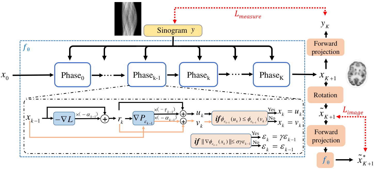
We unrolled the learned descent algorithm in several phases as shown in Fig.1. In each phase $k-1$, we apply the proximal gradient step in Eq.8:

where the proximal operator is defined as:

In order to have a close form solution of the proximal operator, we perform a Taylor approximation of $P_{\varepsilon_{k-1}}$:

After discarding higher-order constant terms, we can simplify the Eq.10 as:

where $\alpha_{k-1}$ and $\beta_{k-1}$ are two parameters greater than 0 and ${\tau_{k-1}}=\frac{{{\alpha_{k-1}}{\beta_{k-1}}}}{{{\alpha_{k-1}}+{\beta_{k-1}}}}$. We also calculate a close-form safeguard $\bm{v}_{k}$ as:

The line search strategy is used by shrinking $\alpha_{k-1}$ to ensure objective function decay. We choose the $\bm{u}_{k}$ or $\bm{v}_{k}$ with smaller objection function value $\phi_{\varepsilon_{k-1}}$ to be the next $\bm{x}_{k}$. The smoothing parameter $\varepsilon_{k-1}$ is shrinkage by $\gamma\in(0,1)$ if the $||\nabla{\phi_{{\varepsilon_{k-1}}}}({\bm{x}_{k}})||<\sigma\gamma{\varepsilon_{k-1}}$ is satisfied. The whole flow is shown in Algorithm 1.

The whole reconstruction network is indicated by $f_{\theta}$ with learned parameter $\theta$. Inspired by Deep image prior [20] and equivariance [18] of PET imaging system, the proposed dual-domain unsupervised training loss function is formulated as:

where $\lambda$ is the parameter that controls the ratio of different domain loss function, which was set to 0.1 in the experiments. For image domain loss $L_{image}$, the equivariance constraint is used. For example, if the test sample $x_{t}$ first undergoes an equivariant transformation, such as rotation, we obtain $x_{tr}$. Subsequently, we perform a PET scan to obtain the sinogram data of $x_{tr}$ and $x_{t}$. The image reconstructed by the $f_{\theta}$ of these two sinogram should also keep this rotation properties. The $L_{image}$ is formulate as:

where $T_{r}$ denotes the rotation operator, $A$ is the forward projection which also can be seen as a measurement operator. For sinogram domain loss $L_{measure}$, the data argumentation with random noise $\bm{\xi}$ is performed on $\bm{y}$:

We implemented DULDA using Pytorch 1.7 on a NVIDIA GeForce GTX Titan X. The Adam optimizer with a learning rate of $10^{-4}$ was used and trained for 100 epochs with batch size of 8. The total unrolled phase was 4. The image $x_{0}$ was initialized with the values of one. The smoothing parameter $\varepsilon_{0}$ and $\delta$ were initialized to be 0.001 and 0.002. The step-size $\alpha_{0}$ and $\beta_{0}$ were initialized to be 0.01 and 0.02. The system matrix was computed by using Michigan Image Reconstruction Toolbox (MIRT) with a strip-integral model [21]. The proposed DULDA was compared with MLEM [22], total variation regularized EM (EM-TV) [23] and deep image prior method (DIP) [16]. For both MLEM and EM-TV, 25 iterations were adopted. The penalty parameter for EM-TV was $2e^{-5}$. For DIP, we used random noise as input and trained 14000 epochs with the same training settings as DULDA to get the best results before over-fitting.

Forty 128$\times$128$\times$40 3D Zubal brain phantoms [24] were used in the simulation study as ground truth, and one clinical patient brain images with different dose level were used for the robust analysis. Two tumors with different size were added in each Zubal brain phantom. The ground truth images were firstly forward-projected to generate the noise-free sinogram with count of $10^{6}$ for each transverse slice and then Poisson noise were introduced. 20 percent of uniform random events were simulated. In total, 1600 (40$\times$40) 2D sinograms were generated. Among them, 1320 (33 samples) were used in training, 200 (5 samples) for testing, and 80 (2 samples) for validation. A total of 5 realizations were simulated and each was trained/tested independently for bias and variance calculation [15]. We used peak signal to noise ratio (PSNR), structural similarity index (SSIM) and root mean square error (RMSE) for overall quantitative analysis. The contrast recovery coefficient (CRC) [25] was used for the comparison of reconstruction results in the tumor region of interest (ROI) area.

Fig. 2 shows three different slices of the reconstructed brain PET images using different methods. The DIP method and proposed DULDA have lower noise compared with MLEM and EM-TV visually. However, the DIP method shows unstable results cross different slices and fails in the recovery of the small cortex region. The proposed DULDA can recover more structural details and the white matter appears to be more sharpen. The quantitative and bias-variance results are shown in Table 1. We noticed that DIP method performs even worse than MLEM without anatomic priors. The DIP method demonstrates a certain ability to reduce noise by smoothing the image, but this leads to losses in important structural information, which explains the lower PSNR and SSIM. Both DIP method and DULDA have a better CRC and Bias performance compared with MLEM and EM-TV.

References

- [1] Nordberg, A., Rinne, J., Kadir, A. Langström, B.: The use of PET in Alzheimer disease. Nature Reviews Neurology. 6, 78-87 (2010)
- [2] Cui, J., Gong, K., Guo, N., Wu, C., Meng, X., Kim, K., Zheng, K., Wu, Z., Fu, L., Xu, B.: PET image denoising using unsupervised deep learning. European Journal Of Nuclear Medicine And Molecular Imaging. 46 pp. 2780-2789 (2019)
- [3] Onishi, Y., Hashimoto, F., Ote, K., Ohba, H., Ota, R., Yoshikawa, E., Ouchi, Y.: Anatomical-guided attention enhances unsupervised PET image denoising performance. Medical Image Analysis. 74 pp. 102226 (2021)
- [4] Zhu, B., Liu, J., Cauley, S., Rosen, B., Rosen, M.: Image reconstruction by domain-transform manifold learning. Nature. 555, 487-492 (2018)
- [5] Häggström, I., Schmidtlein, C., Campanella, G., Fuchs, T.: DeepPET: A deep encoder–decoder network for directly solving the PET image reconstruction inverse problem. Medical Image Analysis. 54 pp. 253-262 (2019)
- [6] Li, Y., Hu, J., Sari, H., Xue, S., Ma, R., Kandarpa, S., Visvikis, D., Rominger, A., Liu, H., Shi, K.: A deep neural network for parametric image reconstruction on a large axial field-of-view PET. European Journal Of Nuclear Medicine And Molecular Imaging. 50, 701-714 (2023)
- [7] Gong, K., Guan, J., Kim, K., Zhang, X., Yang, J., Seo, Y., El Fakhri, G., Qi, J., Li, Q.: Iterative PET image reconstruction using convolutional neural network representation. IEEE Transactions On Medical Imaging. 38, 675-685 (2018)
- [8] Kim, K., Wu, D., Gong, K., Dutta, J., Kim, J., Son, Y., Kim, H., El Fakhri, G., Li, Q.: Penalized PET reconstruction using deep learning prior and local linear fitting. IEEE Transactions On Medical Imaging. 37, 1478-1487 (2018)
- [9] Li, S., Wang, G.: Deep Kernel Representation for Image Reconstruction in PET. IEEE Transactions On Medical Imaging. 41, 3029-3038 (2022)
- [10] Li, S., Gong, K., Badawi, R., Kim, E., Qi, J., Wang, G. Neural KEM: A kernel method with deep coefficient prior for PET image reconstruction. IEEE Transactions On Medical Imaging. (2022)
- [11] Mehranian, A., Reader, A. Model-based deep learning PET image reconstruction using forward–backward splitting expectation–maximization. IEEE Transactions On Radiation And Plasma Medical Sciences. 5, 54-64 (2020)
- [12] Lim, H., Chun, I., Dewaraja, Y., Fessler, J. Improved low-count quantitative PET reconstruction with an iterative neural network. IEEE Transactions On Medical Imaging. 39, 3512-3522 (2020)
- [13] Hu, R., Liu, H.: TransEM: Residual Swin-Transformer based regularized PET image reconstruction. Medical Image Computing And Computer Assisted Intervention–MICCAI 2022: 25th International Conference, Singapore, September 18–22, 2022, Proceedings, Part IV. pp. 184-193 (2022)
- [14] Gong, K., Wu, D., Kim, K., Yang, J., Sun, T., El Fakhri, G., Seo, Y. & Li, Q. MAPEM-Net: an unrolled neural network for Fully 3D PET image reconstruction. 15th International Meeting On Fully Three-dimensional Image Reconstruction In Radiology And Nuclear Medicine. 11072 pp. 109-113 (2019)
- [15] Gong, K., Catana, C., Qi, J., Li, Q.: PET image reconstruction using deep image prior. IEEE Transactions On Medical Imaging. 38, 1655-1665 (2018)
- [16] Hashimoto, F., Ote, K., Onishi, Y.: PET image reconstruction incorporating deep image prior and a forward projection model. IEEE Transactions On Radiation And Plasma Medical Sciences. 6, 841-846 (2022)
- [17] Shen, C., Xia, W., Ye, H., Hou, M., Chen, H., Liu, Y., Zhou, J., Zhang, Y. Unsupervised Bayesian PET Reconstruction. IEEE Transactions On Radiation And Plasma Medical Sciences. (2022)
- [18] Chen, D., Tachella, J., Davies, M.: Robust equivariant imaging: a fully unsupervised framework for learning to image from noisy and partial measurements. Proceedings Of The IEEE/CVF Conference On Computer Vision And Pattern Recognition. pp. 5647-5656 (2022)
- [19] Chen, Y., Liu, H., Ye, X., Zhang, Q.: Learnable descent algorithm for nonsmooth nonconvex image reconstruction. SIAM Journal On Imaging Sciences. 14, 1532-1564 (2021)
- [20] Ulyanov, D., Vedaldi, A., Lempitsky, V.: Deep image prior. Proceedings Of The IEEE Conference On Computer Vision And Pattern Recognition. pp. 9446-9454 (2018)
- [21] Noh, J., Fessler, J., Kinahan, P.: Statistical sinogram restoration in dual-energy CT for PET attenuation correction. IEEE Transactions On Medical Imaging. 28, 1688-1702 (2009)
- [22] Shepp, L. , Vardi, Y.: Maximum likelihood reconstruction for emission tomography. IEEE Transactions on Medical Imaging. 1, 113-122 (1982)
- [23] Jonsson, E., Huang, S., Chan, T. Total variation regularization in positron emission tomography. CAM Report. 9848 (1998)
- [24] Zubal, I., Harrell, C., Smith, E., Rattner, Z., Gindi, G., Hoffer, P.: Computerized three-dimensional segmented human anatomy. Medical Physics. 21, 299-302 (1994)
- [25] Qi, J., Leahy, R.: A theoretical study of the contrast recovery and variance of MAP reconstructions from PET data. IEEE Transactions On Medical Imaging. 18, 293-305 (1999)