Nucleosynthesis of binary-stripped stars. mesaPlot (Farmer 2018), mesaSDK (Townsend 2019), ipython/jupyter (Pérez & Granger 2007; Kluyver et al. 2016), matplotlib (Hunter 2007), NumPy (van der Walt et al. 2011), Parallel (Tange 2021), VICE (Johnson & Weinberg 2020; Johnson et al. 2021; Griffith et al. 2021), MESA(Paxton et al. 2011; Paxton et al. 2013; Paxton et al. 2015; Paxton et al. 2018; Paxton et al. 2019; Jermyn et al. 2022), pyMesa (Farmer & Bauer 2018), and Webplotdigitizer (Rohatgi 2022).

Our explosion models follow those of Farmer et al. 2021. We first excise the the inner region of each star’s core, by placing the inner boundary of our model at the point where the entropy per baryon $\rm{S}=4$ (Brown & Woosley 2013). We then use a thermal bomb, placed at the inner boundary of the model to inject energy into the star (Aufderheide et al. 1991; Sawada & Maeda 2019). We do not allow the model to collapse further inwards after the excising the core, which can alter the final nucleosynthetic signal (Imasheva et al. 2023). In our default model, energy is then injected over the inner $0.01\,\rm{M}_{\odot}$ and over 0.0045 seconds. We inject sufficient energy to bring the total energy of the star (the sum of the kinetic plus thermal energy minus the gravitational binding energy) to $10^{51}\rm{erg/s}$. While there is some evidence for choosing different explosion parameters between stripped envelope supernovae and non-stripped supernovae (Saito et al. 2022), we chose to use a constant set of parameters to minimise the parameter space explored. In Section V.4 we show the uncertainty introduced into the final yields due to differences in the explosion parameters.

The energy we inject into the star is sufficient to drive a hydrodynamic shock that travels outwards from the center of our model to the surface. We stop our models once the shock reaches $0.1\,\rm{M}_{\odot}$ below the surface. In Farmer et al. 2021 we found that the final total energy of a star would be 5--20% higher than what was injected into the star during the explosion. This was due to the change in the nuclear networks (between the end of the stellar evolution and the start of the supernovae) introducing new isotopes that were not in nuclear statistical equilibrium (NSE)²² 2 MESA does not assume NSE, instead it uses the same nuclear network integration that is used at lower temperatures (Paxton et al. 2015). In this work, as we have used the same nuclear network for the entire stars evolution, the core maintains NSE between the stellar evolution and core collapse phases. The difference in final total energy of the star compared to the total energy after the energy injection phase is now $<1\%$.

Many of the isotopes in our 162 isotope nuclear network are short-lived radioactive isotopes and thus would not be expected to contribute to the Galactic yields. Therefore, we also compute the set of stable isotopes converting each radioactive isotope into its single most probable decay product (Timmes, F., priv. com.). This is effectively assuming that we observe the isotopes on a timescale much longer than their half-lives, and that each isotope has only one decay channel³³ 3 This assumption is reasonable for most isotopes in our network except for $\mathrm{{}^{36}Cl}$, $\mathrm{{}^{46}Sc}$, $\mathrm{{}^{54}Mn}$, $\mathrm{{}^{58}Co}$, $\mathrm{{}^{64}Cu}$ where additional decay channels can play a role..

Figure 1 shows that the pre-supernovae mass loss contributes almost the entirety of the chemical yields for low-mass elements. For higher-mass elements, massive binary-stripped stars are able to eject $\approx 20\%$ of their total ejecta in iron-group elements, while for massive single stars this is closer to $\approx 10\%$. This occurs due to the increased mass loss in the binary-stripped stars exposing the He-core during core helium burning. This material is enriched in neutron capture isotopes (see also the much larger contribution of the binary pre-SN mass loss in Figure 1a). These neutrons come primarily from $\mathrm{{}^{22}Ne}\left(\alpha,n\right)\mathrm{{}^{25}Mg}$ (Prantzos et al. 1987). See Appendix C for a discussion of the sensitivity of the isotopic yields due to the wind-scaling factor, and hence total wind mass loss.

We can divide the yields into 3 broad categories: 1) those that change approximately linearly with mass lost (e.g. $\mathrm{{}^{1}H}$, $\mathrm{{}^{4}He}$) either positively or negatively; 2) those that are small or negative until the star exposes its helium core (e.g. $\mathrm{{}^{12}C}$ or $\mathrm{{}^{19}F}$) before increasing; 3) those that fall into neither of those categories, which we discuss below.

Farmer et al. 2021 showed that the mass transferred during Case B RLOF stripping is not enriched in $\mathrm{{}^{12}C}$ compared to the initial abundances, however the structural changes caused by the extra mass loss would affect the star’s evolution, and thus the final $\mathrm{{}^{12}C}$ yield. This was due to the fact that $\mathrm{{}^{12}C}$ was primarily produced during core helium burning which occurred after mass transfer finished.

However, there are also a number of isotopes that are produced in hydrogen envelopes and thus can be ejected during the mass transfer process. These are generally light elements that are either produced in the low temperature environment of the hydrogen envelope or are able to be mixed out of the hydrogen core/shell into the envelope and then ejected.

Figure 1(b) shows similar total ejecta from single and binary-stripped massive stars. However, the net contribution to the Universe will be reduced in the binary-stripped stars as compared to single stars, as their contribution to the composition of the Universe will depend sensitively on how conservative mass transfer is and how the secondary reprocesses and re-ejects any accreted material. We assume for the calculation of the RLOF phase that all the material we eject from the donor accretes onto the accretor (fully conservative). However, we track these isotopes separately and can infer what the composition might be if some fraction of this accreted material is ejected during RLOF or is re-ejected later by the accretor without further nuclear processing as a wind. We will note when we include the contribution from RLOF (or not). Overall, for elements Phosphorus (Z=15) and heavier, the absolute yields from RLOF are $<1\%$ of the absolute wind yields. While for lighter elements the absolute RLOF yields can be comparable to the absolute wind yields.

Figure 2 shows the relative contribution to the IMF-weighted yield from pre-SN mass loss, due to RLOF and stellar winds. Red regions signify that the isotope is predominately ejected in stellar winds, while blue signifies that the isotope is predominately ejected during RLOF. The blue regions show that $\mathrm{{}^{13}C}$, $\mathrm{{}^{14}N}$, and $\mathrm{{}^{21}Ne}$ are primarily ejected during RLOF (we ignore $\mathrm{{}^{7}Be}$ from this discussion, see section VI.2).

As the hydrogen-burning core recedes it will leave behind CNO processed material, allowing the envelope to be enriched in $\mathrm{{}^{14}N}$ which is then ejected during RLOF. The NeNa-cycle is able to convert hydrogen to helium (similar to the CNO cycle) via neon, sodium, and magnesium. Above temperatures of $T>3.5\times 10^{7}$K $\mathrm{{}^{21}Ne}$ is destroyed via $\mathrm{{}^{21}Ne}\left(p,\gamma\right)\mathrm{{}^{22}Na}\left(\beta^{+}\right)\mathrm{{}^{22}Ne}$, while below this temperature $\mathrm{{}^{21}Ne}$ is produced via $\mathrm{{}^{20}Ne}\left(p,\gamma\right)\mathrm{{}^{21}Na}\left(\beta^{+}\right)\mathrm{{}^{21}Ne}$ (Wiescher & Langanke 1986; José et al. 1999). The amount of $\mathrm{{}^{21}Ne}$ is maximised when there is H burning in the temperature range $3\leq T/10^{7}\rm{K}\leq 3.5$ (Arnould et al. 1999). Thus significant amounts of $\mathrm{{}^{21}Ne}$ can only be ejected if the material is burnt in the H-shell and mixed outwards before the H-shell can further process the material.

$\mathrm{{}^{13}C}$ can provide a significant fraction of the neutron flux at stellar densities and temperatures, via the reaction $\mathrm{{}^{13}C}\left(\alpha,n\right)\mathrm{{}^{16}O}$ (Busso et al. 1999), thus its production (and destruction) plays a key role in the s-process (Gallino et al. 1998). The ratio of $\mathrm{{}^{12}C}$/$\mathrm{{}^{13}C}$ has also been used as a a probe of galactic chemical evolution (Milam et al. 2005).

Table 1 shows the IMF weighted $\mathrm{{}^{12}C}$/$\mathrm{{}^{13}C}$ ratio from the different mass loss processes. The totals show the $\mathrm{{}^{12}C}$/$\mathrm{{}^{13}C}$ ratio depending on whether the mass donated by the primary is ejected from the system (with RLOF) or is assumed to be accreted onto the accretor and mixed inwards (without RLOF), thus not being ejected into the Universe. This assumes the accretor does not re-eject the material at a later time. Table 1 therefore indicates that the contribution to the Galactic $\mathrm{{}^{12}C}$/$\mathrm{{}^{13}C}$ from massive stars will depend sensitivity on how conservative mass transfer is, thus how much mass is accreted, and whether the accretor re-ejects the material or it is mixed into the core. Thus the $\mathrm{{}^{12}C}$/$\mathrm{{}^{13}C}$ ratio in regions where the dominant enrichment is from massive stars could potentially be used as a tracer of how conservative mass transfer is, as the ejection of $\mathrm{{}^{13}C}$ occurs primarily during the mass transfer process, while $\mathrm{{}^{12}C}$ is primarily ejected from WR wind mass loss.

The Solar system has $\mathrm{{}^{12}C}$/$\mathrm{{}^{13}C}$$\approx 90$ (Romano et al. 2019; Botelho et al. 2020), which is lower than the values in Table 1, thus the primary producer of $\mathrm{{}^{13}C}$ is likely lower-mass stars, for instance AGB and TP-AGB stars which can have $\mathrm{{}^{12}C}$/$\mathrm{{}^{13}C}$ values between $\sim 10$–$180$ depending on the initial mass (Karakas & Lugaro 2016).

The final fate of a star depends on many quantities, however the core mass and the central $\mathrm{{}^{12}C}$ fraction at the end of core helium burning are two of the most important (Chieffi & Limongi 2020; Patton & Sukhbold 2020). Figure 3 shows a comparison of the core $\mathrm{C}$ fraction at the end of core helium depletion for various solar metallicity models. In general we can see that as the initial mass increases, the core $\mathrm{{}^{12}C}$ fraction decreases. It is set by the combination of the $3\alpha$ rate and the ${}^{12}\rm{C}\left(\alpha,\gamma\right)^{16}\!\rm{O}$ reaction (Sukhbold & Adams 2020). For our single star models, the $\mathrm{{}^{12}C}$ fraction agrees well with Schneider et al. 2021, which is unsurprising as Schneider et al. 2021 also used MESA with similar physics choices, although there is a divergence at high initial mass, which may be due to our different choices of chemical mixing. Schneider et al. 2021 also uses a similar wind prescription as this work, but with a different dependence on the metallicity.

Our binary-stripped models also closely match the values of Schneider et al. 2021 case-B binaries, with differences likely due to the different method of removing the envelope, as Schneider et al. 2021 takes the material off with an ad-hoc prescription, while we follow the binary mass transfer. Our models show a variability in the $\mathrm{{}^{12}C}$ trend, not seen in Schneider et al. 2021, in the 20–30$\,\rm{M}_{\odot}$ mass range. This is where both the MLT++ approximation is important and the envelope is not significantly removed by winds before mass transfer begins. Thus the envelopes properties depend sensitively on the ad-hoc MLT++ prescription, which propagates as an uncertainty in how wind mass loss occurs, and how efficient RLOF is at removing the envelope. How mass is lost from a star has been shown to significantly impact the internal structure of massive stars (Renzo et al. 2017).

Our binary-stripped models also agree well with the Chieffi & Limongi 2020 single star models, for $\rm{M_{init}}<20\,\rm{M}_{\odot}$. Both Chieffi & Limongi 2020 and this work use NACRE (Angulo et al. 1999) for the 3$\alpha$ rate. For the ${}^{12}\rm{C}\left(\alpha,\gamma\right)^{16}\!\rm{O}$ rate Chieffi & Limongi 2020 uses Kunz et al. 2002 while we use Angulo et al. 1999 rate. Therefore differences likely stem from different choices in the nuclear physics. Thus binary stripping has a similar effect on the core abundance as variations in the ${}^{12}\rm{C}\left(\alpha,\gamma\right)^{16}\!\rm{O}$ reaction rate.

As shown extensively in Laplace et al. 2021 the effect of the extra mass loss due to RLOF causes structural changes to the cores of massive stars. These changes cause the cores to become smaller (in mass) and to have extended chemical gradients. This leads to differences in the intensity and timing of nuclear shell burning episodes, which compounds the differences between single and binary-stripped stars. While Farmer et al. 2021 has shown how the binary interactions affect the final $\mathrm{{}^{12}C}$ yield.

Details of key stellar properties can be found in Appendix D and in Tables 3 and 4. These include the final total and core mass, total mass lost to different mass loss processes, and final masses of H, He, and C.

We first determine whether a star will successfully explode and eject its envelope, or not. Figure 4 shows two measures of a star’s explodability: its compactness (O’Connor & Ott 2011) (y-axis) and the two component fit of Ertl et al. 2016 (symbols), as a function of the initial mass. As shown in many other works (Sukhbold et al. 2016; Farmer et al. 2016; Renzo et al. 2017; Sukhbold & Adams 2020; Patton & Sukhbold 2020, e.g.), the evolution to core collapse and the star’s final structure is sensitive to the choice of physics, treatment of chemical mixing boundaries (Chieffi & Limongi 2020), and numerical choices (Farmer et al. 2016) made by the software instrument used. In Figure 4 we define three regions based on the two component fit of Ertl et al. 2016⁴⁴ 4 See also Boccioli et al. 2022 for a potential new criterion for determining explodability. One region contains models that only make NSs ($\xi_{M=2.5}\leq 0.16$), another contains those that only make BHs ($\xi_{M=2.5}\geq 0.36$), and there is an intermediate region in which we consider the outcomes to be less certain. The boundaries of these regions are almost the same as the boundaries found by Ugliano et al. 2012 ($\xi_{M=2.5}\leq 0.15$ for NS and $\xi_{M=2.5}\geq 0.35$ for BH). But the presence of the mixed region shows why the compactness, on its own, is not a good measure for determining the explosion outcome.

In Figure 4 we can find several regions that are expected to undergo successful explosions, with only slight movement of the boundaries between single and binary stars. Between $11<\rm{M_{init}}/\,\rm{M}_{\odot}<21$ and $31<\rm{M_{init}}/\,\rm{M}_{\odot}<36$ stars end their lives with similar compactness parameters (and with similar explosion success metrics). In contrast, between $21<\rm{M_{init}}/\,\rm{M}_{\odot}<31$ (though there are a number of missing models here) and $\rm{M_{init}}>38\,\rm{M}_{\odot}$ the final states of the stars are very different between single and binary-stripped stars, leading to differences both in the explodability and their final nucleosynthetic yields.

The structure seen in Figure 4 is related to the transition in how different fuels ignite in the core (Sukhbold & Woosley 2014; Laplace et al. 2021). The peak at $\rm{M_{init}}\approx 25\,\rm{M}_{\odot}$ is when carbon changes from central to off-center burning while the peak at $\rm{M_{init}}\approx 34\,\rm{M}_{\odot}$ is coincident with neon going from central to off-center burning (Schneider et al. 2021). The shift in the location of the peaks between binary-stripped and single stars is due to the binary-stripped stars having smaller core masses, due to the core receding when RLOF removed the envelope (Farmer et al. 2021).

We include the fallback prescription of Goldberg et al. 2019. Here zones near the inner boundary are removed that have a total energy, when integrated from the core to the zone, that is negative. This is done by moving the inner boundary of the model to the point where the material has a positive total energy, and thus is unbound from the core. This is repeated at each time step. See Appendix A of Goldberg et al. 2019 and Paxton et al. 2015 for the full details of this fallback treatment. For the models presented here and with our default explosion parameters, the amount of fallback is negligible ($\Delta\rm{M}\lessapprox 10^{-3}\,\rm{M}_{\odot}$) even in cases that do not formally explode via the Ertl et al. 2016 criterion. As the amount of fallback is negligible in these models, for the choices of explosion physics used here, we simplify our modelling by using an explodability criterion. This lack of fallback is driven by our choice of a fixed $10^{51}\rm{erg/s}$ explosion, lower energy explosions can have larger fallback masses with the prescription as implemented in MESA (Goldberg et al. 2019).

Schneider et al. 2021 found that for case B binaries (where they artificially remove the envelope), NS production occurs for $\rm{M_{init}}\leq 31.5\,\rm{M}_{\odot}$ and $\rm{M_{init}}>34.0\,\rm{M}_{\odot}$, while for single stars the range is between $\rm{M_{init}}\leq 21.5\,\rm{M}_{\odot}$ and $23.5\leq\rm{M_{init}}/\,\rm{M}_{\odot}\leq 34.0$. These boundaries can shift if fallback accretion is taken into account (Timmes et al. 1996). We find a somewhat more complex boundary between NS and BH formation for $\rm{M_{init}}\leq 22\,\rm{M}_{\odot}$ and $\rm{M_{init}}>36\,\rm{M}_{\odot}$. Differences between the boundaries found by Schneider et al. 2021 and those in this work are likely due to differences in the physical assumptions, such as the choice of convective boundary mixing, timing of mass loss, and the choice of nuclear network. These have been shown to lead to large changes in the final structure (Farmer et al. 2016; Renzo et al. 2017; Farmer et al. 2021).

Figure 5 shows a comparison between our 13$\,\rm{M}_{\odot}$ single⁵⁵ 5 Formally our 13$\,\rm{M}_{\odot}$ single star does not explode by any of the fits provided in Ertl et al. 2016, however given the limited range of initial masses in Limongi & Chieffi 2018 that overlap with our models, we chose this initial mass as the binary-stripped model comfortably forms a NS, while both the 15$\,\rm{M}_{\odot}$ models are on the edge between NS and BH, the 20$\,\rm{M}_{\odot}$ models both make BHs, and we have no model for a 25$\,\rm{M}_{\odot}$ stripped-binary. and binary-stripped stars with yields available in the literature⁶⁶ 6 We made use of the VICE (Johnson & Weinberg 2020; Johnson et al. 2021; Griffith et al. 2021) software package to provide this information.. Panel (a) shows the total elemental yields (as a sum of the stable isotopes), while Panel (b) shows the ratio of the elemental yield for our single star model as compared to the literature values. Our supernova models were exploded with our default explosion physics.

Overall, we over predict (as compared to the literature) elements in the Z=10–21 range by a factor of 5. For higher mass elements we have a good agreement with the Kepler based results (Sukhbold et al. 2016; Woosley 2018) while diverging to a factor 10 over prediction compared to the results of (Limongi & Chieffi 2018) which are based on the FRANEC code. Our large disagreement for Zinc is due to the fact that our nuclear network stops at Zinc, thus isotopes will pile up at the edge unable to produce heavier isotopes. Other differences are likely due to differences in the stellar micro-physics and physical assumptions. For instance, we showed in Farmer et al. 2021 that the, currently unconstrained, choice for the amount of overshoot during carbon burning can have a significant impact on the carbon yields, that would then propagate as an uncertainty on the product of carbon burning namely $\mathrm{{}^{20}Ne}$, $\mathrm{{}^{23}Na}$, and $\mathrm{{}^{24}Mg}$. This is due to a $\mathrm{{}^{12}C}$ yield being sensitive to the size of the pocket of $\mathrm{C}$ that survives, between the top of the final carbon-burning shell and the helium shell (Farmer et al. 2021). This pocket, however, can be eroded by convective overshoot from the final convective carbon-burning shells.

Figure 5b also shows the comparison between a binary-stripped model and a single star model, for the same initial mass. Here we can see that the binary-stripped model produces more of the intermediate-mass elements ($15<Z<24$) by up to a factor $\approx 4$, while producing slightly less of the higher mass elements ($Z>24$), as well as producing less magnesium and aluminum (Z=12 and Z=13).

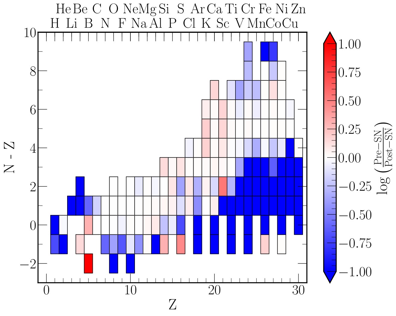
Figure 6 shows the relative change in the IMF-weighted material ejected in a SN between its pre-SN composition and its post-SN composition. Blue regions indicate isotopes that are produced in the SN while red regions indicate isotopes that are destroyed in the SN. The color bar has been truncated, to better show the details, however the (blue) material produced can peak at $\approx 10^{15}$ times more (for isotopes in the bottom right corner), and the (red) material destroyed peaks at only $\approx 10^{4}$ times less.

We can see in Figure 6 that most of the region of change occurs for $Z>20$ and $N-Z<4$. These are generally the proton-rich isotopes, that have very low abundances outside of the mass cut pre-SN. Thus even a small production during the SN causes a large relative increase in the composition. There is also an increase in the more neutron rich isotopes, typically expected for r-process, in the top right of each panel in Figure 6. This includes the isotope $\mathrm{{}^{60}Fe}$ which is of interest for gamma-ray observations (Mahoney et al. 1982; Leising & Share 1994).

Comparing Figures 6(a) to 6(b), we can see that both show this enhancement in proton-rich isotopes, though the single stars show a greater fraction of material coming from the pre-SN evolution for the most proton-rich isotopes of Ti, Cr, and Fe. For the more neutron-rich isotopes ($N-Z\approx 8$), the single stars show material coming more from the explosive nucleosynthesis during the SN than before. For neutron-rich isotopes of Al–Sc, binary-stripped stars are generally producing this material pre-SN (and outside what will becomes the compact object), while in single stars this occurs during the explosive nucleosynthesis in the SN.

We reconfirm our finding the $\mathrm{{}^{12}C}$ is not affected by the supernova shock (Farmer et al. 2021). We find, with our larger number of isotopes, that $\mathrm{{}^{12}C}$ is in fact the isotope least affected by the supernova explosion. This is due both to its location near the He-shell, thus little $\mathrm{{}^{12}C}$ is lost to the formation of the compact object, and when the shock finally reaches the He-shell it has cooled sufficiently to be unable to drive additional $\mathrm{{}^{12}C}$ burning.

Following the method of Farmer et al. 2021 we explore the sensitivity of our SN yields to the uncertain explosion physics. We took a 17$\,\rm{M}_{\odot}$⁷⁷ 7 Our 17$\,\rm{M}_{\odot}$ single star model does not formally explode given the fits in Ertl et al. 2016, though it does have a similar compactness to the 17$\,\rm{M}_{\odot}$ binary-stripped model. single and binary-stripped star models and exploded each of them $\approx 100$ times. For each sample we would randomly vary the following four parameters: the injection energy, mass cut, injection mass, and injection time. As an improvement over Farmer et al. 2021 we sample all four explosion parameters simultaneously as opposed to doing two grids, which sampled only two parameters at a time. We vary the injection energy between $0.5$–$5.0\times 10^{51}\rm{erg/s}$, the mass cut between $1.0$–$2.0\,\rm{M}_{\odot}$, the injection mass $10^{-2}$–$5\times 10^{-1}\,\rm{M}_{\odot}$, and the injection time $10^{-3}$–1.0s. We assume a thermal bomb for our explosions, however a piston driven explosion may produce different yields for the same input energy (Young & Fryer 2007).

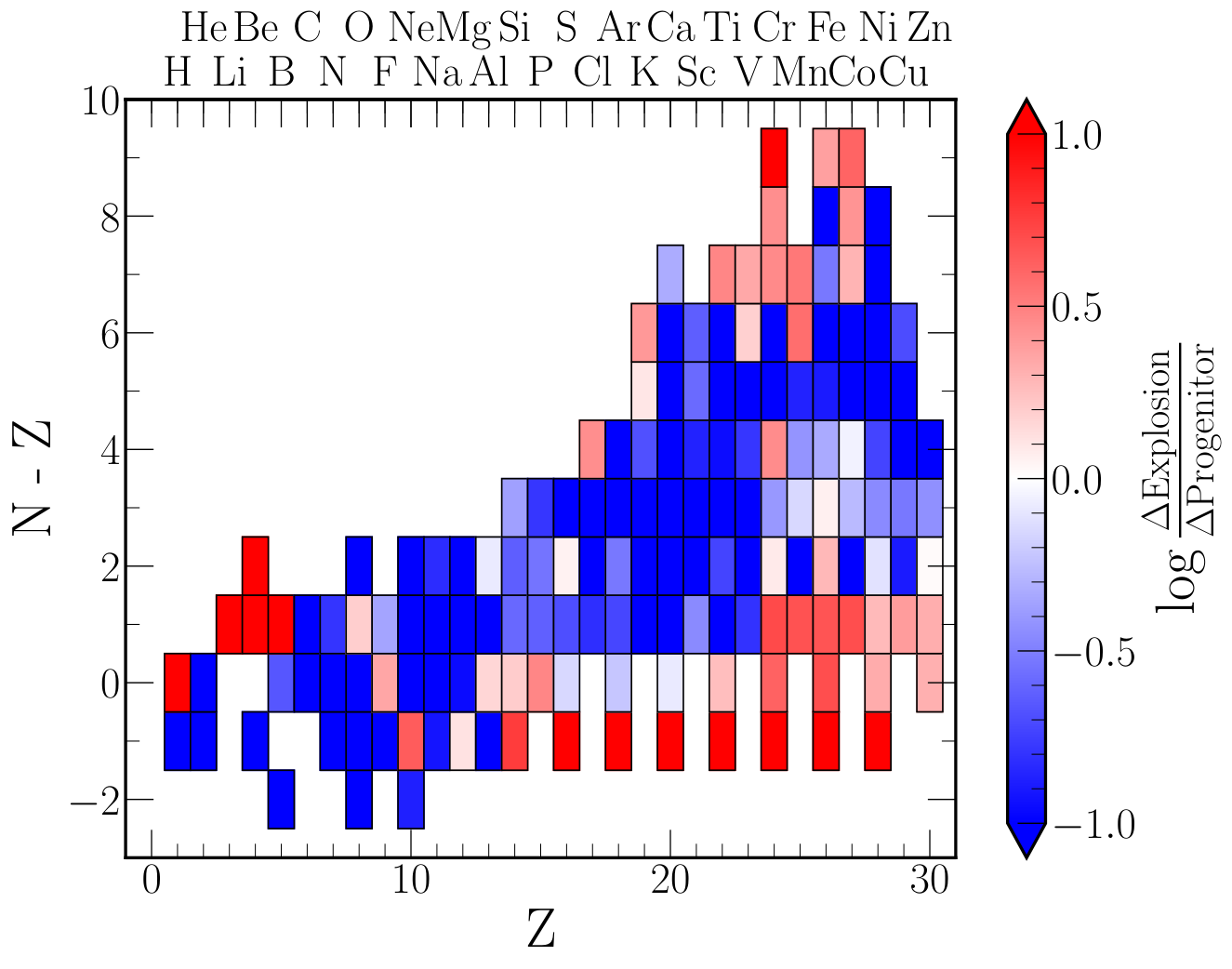
Figure 7 shows for which isotopes it is more important to understand the progenitor ($\log\left(\Delta\rm{Explosion}/\Delta\rm{Progenitor}\right)=-1.0$) and for which isotopes it is more important to understand the explosion mechanism ($\log\left(\Delta\rm{Explosion}/\Delta\rm{Progenitor}\right)>-1.0$ ). Where $\Delta\rm{Explosion}$ is the spread in the final ejecta composition for a 17$\,\rm{M}_{\odot}$ model where we vary the explosion physics, and $\Delta\rm{Progenitor}$ is the spread in the final ejecta composition for fixed explosion physics but considering our entire range of initial masses. Both $\Delta\rm{Explosion}$ and $\Delta\rm{Progenitor}$ are defined separately for our single and binary-stripped stars.

Figure 7 also shows that there is a difference between single stars and binary-stripped stars in which isotopes are uncertain, and thus which types of supernovae could be used to constrain different isotopes if detectable either through spectroscopy or radioactive decay signatures. These differences occur due to the differences in the time needed for the shock to break out of the photosphere, in the less massive single stars (which still have a RSG envelope) shock breakout is approximately a day after the core collapses, while in our binary-stripped stars (and high-mass single stars that lose their H-envelopes) shock breakout occurs much less than a day after the core collapses. Thus stripped-envelope supernovae explode faster and have less time for short lived radioactive nuclei to decay before the shock breakout phase. This hints that stripped-envelope supernovae from binaries could be interesting locations to study radioactive decay products from explosive nucleosynthesis, with sufficiently early time observations and sufficient chemical mixing to bring them to the photosphere.

In Andrews et al. 2020 a number of isotopes ($\mathrm{{}^{43}K}$, $\mathrm{{}^{47}Ca}$, $\mathrm{{}^{44}Sc}$, $\mathrm{{}^{47}Sc}$, $\mathrm{{}^{48}V}$, $\mathrm{{}^{48}Cr}$, $\mathrm{{}^{51}Cr}$, $\mathrm{{}^{52}Mn}$, $\mathrm{{}^{59}Fe}$, $\mathrm{{}^{56}Co}$, $\mathrm{{}^{57}Co}$, and $\mathrm{{}^{57}Ni}$) were determined to be interesting candidates for next-generation gamma-ray detectors. This was due to their accessible gamma-ray energies as well as their sensitivity to the structure of the progenitor ($\mathrm{{}^{48}V}$ and $\mathrm{{}^{57}Co}$) or the explosion energy ($\mathrm{{}^{43}K}$, $\mathrm{{}^{47}Ca}$, $\mathrm{{}^{44}Sc}$, $\mathrm{{}^{47}Sc}$, $\mathrm{{}^{59}Fe}$).

If we assume the (arbitrary) point of $\log\left(\Delta\rm{Explosion}/\Delta\rm{Progenitor}\right)>0.1$ as the point where isotopes are probing for the explosion mechanism (instead of them profiling the stellar structure) we can then use the isotope list of Andrews et al. 2020 to determine whether these isotopes are interesting for our binary-stripped stars. We find that the following are interesting isotopes, by that definition, for probing the explosion properties in single stars: $\mathrm{{}^{48}V}$, $\mathrm{{}^{48}Cr}$, $\mathrm{{}^{51}Cr}$, $\mathrm{{}^{52}Mn}$, $\mathrm{{}^{56}Co}$, $\mathrm{{}^{57}Co}$, and $\mathrm{{}^{57}Ni}$, while for binaries it is: $\mathrm{{}^{44}Sc}$, $\mathrm{{}^{48}Cr}$, $\mathrm{{}^{59}Fe}$, $\mathrm{{}^{57}Co}$, and $\mathrm{{}^{57}Ni}$. Note that the two lists do not overlap, nor does each isotope have the same level of sensitivity to the explosion between single and binary-stripped stars. We find $\mathrm{{}^{48}V}$ and $\mathrm{{}^{52}Mn}$ are much stronger probes of the explosion physics in single stars than in binaries, while $\mathrm{{}^{48}Cr}$ is more sensitive to the explosion mechanism in binaries than in singles.

$\mathrm{{}^{26}Al}$ is a short-lived isotope that decays to an excited state of $\mathrm{{}^{26}Mg}$. This excited $\mathrm{{}^{26}Mg}$ then rapidly emits a 1.81 MeV $\gamma$-ray. Given the the short half life of $\mathrm{{}^{26}Al}$, its detection in the Galaxy requires a continuous production source (Diehl et al. 2010). $\mathrm{{}^{26}Al}$ has multiple formation sites inside stars, mainly via proton captures onto $\mathrm{{}^{25}Mg}$ (Limongi & Chieffi 2006). However, $\mathrm{{}^{26}Al}$ has several isomers which complicate the decay chain. The ground state of $\mathrm{{}^{26}Al}$ decays to $\mathrm{{}^{26}Mg}$ with a half life of $\sim 700$ kyr, however the excited state of $\mathrm{{}^{26}Al}$ decays to $\mathrm{{}^{26}Mg}$ in $\sim 6$ seconds (Misch et al. 2021). At the temperatures found in stellar envelopes, excited $\mathrm{{}^{26}Al}$ decays to $\mathrm{{}^{26}Mg}$ before it can de-excite back to its ground state, this rapidly converts most of the $\mathrm{{}^{26}Al}$ into $\mathrm{{}^{26}Mg}$. Our nuclear network does not contain the $\mathrm{{}^{26}Al}$ isomers, with the decay rate of $\mathrm{{}^{26}Al}$ only considering the ground state transitions. Thus we significantly over produce the amount of $\mathrm{{}^{26}Al}$ in our wind yields and RLOF ejecta (see for instance the models of Brinkman et al. 2019; Brinkman et al. 2021 for $\mathrm{{}^{26}Al}$ yields from binary stars). This over production ranges from a factor 10 to 10,000 depending on the initial mass, with low mass stars having larger overproduction factors. Thus we can make no statement on the production of $\mathrm{{}^{26}Al}$ in stellar winds, without further post-processing of the chemical yields. Tests with a nuclear network that contains the $\mathrm{{}^{26}Al}$ isomers give wind and RLOF results that are consistent with those of Brinkman et al. 2021. In our models we have $\mathrm{{}^{26}Mg}$ wind yields of $M\approx 10^{-3}\,\rm{M}_{\odot}$, while $\mathrm{{}^{26}Al}$ wind yields of $M\approx 10^{-4}\,\rm{M}_{\odot}$ (at $\rm{M_{init}}\approx 20\,\rm{M}_{\odot}$). Thus the lack of $\mathrm{{}^{26}Al}$ excited-state decays to $\mathrm{{}^{26}Mg}$ leads to a systematic change of order 10% (depending on the initial stellar mass) in the $\mathrm{{}^{26}Mg}$ wind yields.

MESA’s default reaction rate for $\mathrm{{}^{7}Be}(e^{-},\nu_{e})\mathrm{{}^{7}Li}$ (for version r12115) came from REACLIB (Cyburt et al. 2010). However, REACLIB is only defined for temperatures above $T>10^{7}$K, thus it assumes that all atoms are ionised. While this is a reasonable assumption for most rates, which occur deep in the stellar interior, significant lithium production occurs in stellar envelopes with temperatures below $T<10^{7}$K where the reaction rate can then depend on the level of ionisation (Schwab 2020). This has been corrected in MESA version 2c2ad6c by switching to the rate of Simonucci et al. 2013 which includes this effect, but this was not available in MESA for this work. We caution against making any inferences for either $\mathrm{{}^{7}Be}$ or $\mathrm{{}^{7}Li}$ from this work. Other isotopes that are sensitive to the level of ionisation may also be affected, if their rates are provided by REACLIB.

References

- Aadland et al. (2022) Aadland, E., Massey, P., John Hillier, D., et al. 2022, ApJ, 931, 157, doi: 10.3847/1538-4357/ac66e7
- Abate et al. (2015) Abate, C., Pols, O. R., Karakas, A. I., & Izzard, R. G. 2015, A&A, 576, A118, doi: 10.1051/0004-6361/201424739
- Abt (1983) Abt, H. A. 1983, ARA&A, 21, 343
- Andrews et al. (2020) Andrews, S., Fryer, C., Even, W., Jones, S., & Pignatari, M. 2020, ApJ, 890, 35, doi: 10.3847/1538-4357/ab64f8
- Angulo et al. (1999) Angulo, C., Arnould, M., Rayet, M., et al. 1999, Nucl. Phys. A, 656, 3, doi: 10.1016/S0375-9474(99)00030-5
- Arnould et al. (1999) Arnould, M., Goriely, S., & Jorissen, A. 1999, A&A, 347, 572. https://arxiv.org/abs/astro-ph/9904407
- Arnould et al. (2007) Arnould, M., Goriely, S., & Takahashi, K. 2007, Phys. Rep., 450, 97, doi: 10.1016/j.physrep.2007.06.002
- Arnould & Takahashi (1999) Arnould, M., & Takahashi, K. 1999, Reports on Progress in Physics, 62, 395, doi: 10.1088/0034-4885/62/3/003
- Aufderheide et al. (1991) Aufderheide, M. B., Baron, E., & Thielemann, F. K. 1991, ApJ, 370, 630, doi: 10.1086/169849
- Aufderheide et al. (1994) Aufderheide, M. B., Fushiki, I., Woosley, S. E., & Hartmann, D. H. 1994, ApJS, 91, 389, doi: 10.1086/191942
- Bliss et al. (2020) Bliss, J., Arcones, A., Montes, F., & Pereira, J. 2020, Phys. Rev. C, 101, 055807, doi: 10.1103/PhysRevC.101.055807
- Boccioli et al. (2022) Boccioli, L., Roberti, L., Limongi, M., Mathews, G. J., & Chieffi, A. 2022, arXiv e-prints, arXiv:2207.08361. https://arxiv.org/abs/2207.08361
- Botelho et al. (2020) Botelho, R. B., Milone, A. d. C., Meléndez, J., et al. 2020, MNRAS, 499, 2196, doi: 10.1093/mnras/staa2917
- Braun & Langer (1995a) Braun, H., & Langer, N. 1995a, A&A, 297, 483
- Braun & Langer (1995b) Braun, H., & Langer, N. 1995b, in Wolf-Rayet Stars: Binaries; Colliding Winds; Evolution, ed. K. A. van der Hucht & P. M. Williams, Vol. 163, 305
- Brinkman et al. (2021) Brinkman, H. E., den Hartogh, J. W., Doherty, C. L., Pignatari, M., & Lugaro, M. 2021, ApJ, 923, 47, doi: 10.3847/1538-4357/ac25ea
- Brinkman et al. (2019) Brinkman, H. E., Doherty, C. L., Pols, O. R., et al. 2019, ApJ, 884, 38, doi: 10.3847/1538-4357/ab40ae
- Brott et al. (2011) Brott, I., de Mink, S. E., Cantiello, M., et al. 2011, A&A, 530, A115, doi: 10.1051/0004-6361/201016113
- Brown et al. (2001) Brown, G. E., Heger, A., Langer, N., et al. 2001, New A, 6, 457, doi: 10.1016/S1384-1076(01)00077-X
- Brown et al. (1999) Brown, G. E., Lee, C. H., & Bethe, H. A. 1999, New A, 4, 313, doi: 10.1016/S1384-1076(99)00023-8
- Brown et al. (1996) Brown, G. E., Weingartner, J. C., & Wijers, R. A. M. J. 1996, ApJ, 463, 297, doi: 10.1086/177241
- Brown & Woosley (2013) Brown, J. M., & Woosley, S. E. 2013, ApJ, 769, 99, doi: 10.1088/0004-637X/769/2/99
- Buchler & Yueh (1976) Buchler, J. R., & Yueh, W. R. 1976, ApJ, 210, 440, doi: 10.1086/154847
- Burbidge et al. (1957) Burbidge, E. M., Burbidge, G. R., Fowler, W. A., & Hoyle, F. 1957, Reviews of Modern Physics, 29, 547, doi: 10.1103/RevModPhys.29.547
- Busso et al. (1999) Busso, M., Gallino, R., & Wasserburg, G. J. 1999, ARA&A, 37, 239, doi: 10.1146/annurev.astro.37.1.239
- Carigi et al. (2005) Carigi, L., Peimbert, M., Esteban, C., & García-Rojas, J. 2005, ApJ, 623, 213, doi: 10.1086/428491
- Cassisi et al. (2007) Cassisi, S., Potekhin, A. Y., Pietrinferni, A., Catelan, M., & Salaris, M. 2007, ApJ, 661, 1094, doi: 10.1086/516819
- Cescutti et al. (2009) Cescutti, G., Matteucci, F., McWilliam, A., & Chiappini, C. 2009, A&A, 505, 605, doi: 10.1051/0004-6361/200912759
- Chieffi & Limongi (2004) Chieffi, A., & Limongi, M. 2004, ApJ, 608, 405, doi: 10.1086/392523
- Chieffi & Limongi (2020) —. 2020, ApJ, 890, 43, doi: 10.3847/1538-4357/ab6739
- Chugunov et al. (2007) Chugunov, A. I., Dewitt, H. E., & Yakovlev, D. G. 2007, Phys. Rev. D, 76, 025028, doi: 10.1103/PhysRevD.76.025028
- Crowther (2007) Crowther, P. A. 2007, ARA&A, 45, 177, doi: 10.1146/annurev.astro.45.051806.110615
- Cyburt et al. (2010) Cyburt, R. H., Amthor, A. M., Ferguson, R., et al. 2010, The Astrophysical Journal Supplement Series, 189, 240, doi: 10.1088/0067-0049/189/1/240
- De Donder & Vanbeveren (2004) De Donder, E., & Vanbeveren, D. 2004, New A Rev., 48, 861, doi: 10.1016/j.newar.2004.07.001
- de Jager et al. (1988) de Jager, C., Nieuwenhuijzen, H., & van der Hucht, K. A. 1988, A&AS, 72, 259
- de Mink et al. (2009) de Mink, S. E., Cantiello, M., Langer, N., et al. 2009, A&A, 497, 243, doi: 10.1051/0004-6361/200811439
- de Mink et al. (2013) de Mink, S. E., Langer, N., Izzard, R. G., Sana, H., & de Koter, A. 2013, ApJ, 764, 166, doi: 10.1088/0004-637X/764/2/166
- deBoer et al. (2017) deBoer, R. J., Görres, J., Wiescher, M., et al. 2017, Reviews of Modern Physics, 89, 035007, doi: 10.1103/RevModPhys.89.035007
- Deckers et al. (2021) Deckers, M., Groh, J. H., Boian, I., & Farrell, E. J. 2021, MNRAS, 507, 3726, doi: 10.1093/mnras/stab2423
- Diehl et al. (2022) Diehl, R., Korn, A. J., Leibundgut, B., Lugaro, M., & Wallner, A. 2022, Progress in Particle and Nuclear Physics, 127, 103983, doi: 10.1016/j.ppnp.2022.103983
- Diehl et al. (2010) Diehl, R., Lang, M. G., Martin, P., et al. 2010, A&A, 522, A51, doi: 10.1051/0004-6361/201014302
- Dominik et al. (2012) Dominik, M., Belczynski, K., Fryer, C., et al. 2012, ApJ, 759, 52, doi: 10.1088/0004-637X/759/1/52
- Dominik et al. (2013) —. 2013, ApJ, 779, 72, doi: 10.1088/0004-637X/779/1/72
- Eggleton (1983) Eggleton, P. P. 1983, ApJ, 268, 368, doi: 10.1086/160960
- Eitner et al. (2022) Eitner, P., Bergemann, M., Ruiter, A. J., et al. 2022, arXiv e-prints, arXiv:2206.10258. https://arxiv.org/abs/2206.10258
- Ekström et al. (2012) Ekström, S., Georgy, C., Eggenberger, P., et al. 2012, A&A, 537, A146, doi: 10.1051/0004-6361/201117751
- Eldridge et al. (2008) Eldridge, J. J., Izzard, R. G., & Tout, C. A. 2008, MNRAS, 384, 1109, doi: 10.1111/j.1365-2966.2007.12738.x
- Ertl et al. (2016) Ertl, T., Janka, H. T., Woosley, S. E., Sukhbold, T., & Ugliano, M. 2016, ApJ, 818, 124, doi: 10.3847/0004-637X/818/2/124
- Farmer (2018) Farmer, R. 2018, rjfarmer/mesaplot, doi: 10.5281/zenodo.1441329
- Farmer & Bauer (2018) Farmer, R., & Bauer, E. B. 2018, rjfarmer/pyMesa: Add support for 10398, v1.0.3, Zenodo, doi: 10.5281/zenodo.1205271
- Farmer et al. (2016) Farmer, R., Fields, C. E., Petermann, I., et al. 2016, ApJS, 227, 22, doi: 10.3847/1538-4365/227/2/22
- Farmer et al. (2021) Farmer, R., Laplace, E., de Mink, S. E., & Justham, S. 2021, ApJ, 923, 214, doi: 10.3847/1538-4357/ac2f44
- Farmer et al. (2020) Farmer, R., Renzo, M., de Mink, S. E., Fishbach, M., & Justham, S. 2020, ApJ, 902, L36, doi: 10.3847/2041-8213/abbadd
- Ferguson et al. (2005) Ferguson, J. W., Alexander, D. R., Allard, F., et al. 2005, ApJ, 623, 585, doi: 10.1086/428642
- Fields et al. (2016) Fields, C. E., Farmer, R., Petermann, I., Iliadis, C., & Timmes, F. X. 2016, ApJ, 823, 46, doi: 10.3847/0004-637X/823/1/46
- Fields et al. (2018) Fields, C. E., Timmes, F. X., Farmer, R., et al. 2018, The Astrophysical Journal Supplement Series, 234, 19, doi: 10.3847/1538-4365/aaa29b
- Franchini et al. (2020) Franchini, M., Morossi, C., Di Marcantonio, P., et al. 2020, ApJ, 888, 55, doi: 10.3847/1538-4357/ab5dc4
- Franco et al. (2021) Franco, M., Coppin, K. E. K., Geach, J. E., et al. 2021, Nature Astronomy, 5, 1240, doi: 10.1038/s41550-021-01515-9
- Freiburghaus et al. (1999) Freiburghaus, C., Rosswog, S., & Thielemann, F. K. 1999, ApJ, 525, L121, doi: 10.1086/312343
- Fuller et al. (1985) Fuller, G. M., Fowler, W. A., & Newman, M. J. 1985, ApJ, 293, 1, doi: 10.1086/163208
- Gaia Collaboration et al. (2021) Gaia Collaboration, Brown, A. G. A., Vallenari, A., et al. 2021, A&A, 649, A1, doi: 10.1051/0004-6361/202039657
- Gaia Collaboration et al. (2022) Gaia Collaboration, Recio-Blanco, A., Kordopatis, G., et al. 2022, arXiv e-prints, arXiv:2206.05534. https://arxiv.org/abs/2206.05534
- Gallino et al. (1998) Gallino, R., Arlandini, C., Busso, M., et al. 1998, ApJ, 497, 388, doi: 10.1086/305437
- Goldberg et al. (2019) Goldberg, J. A., Bildsten, L., & Paxton, B. 2019, ApJ, 879, 3, doi: 10.3847/1538-4357/ab22b6
- Goriely et al. (1990) Goriely, S., Jorissen, A., & Arnould, M. 1990, in Nuclear Astrophysics, 5th Workshop, 60
- Götberg et al. (2017) Götberg, Y., de Mink, S. E., & Groh, J. H. 2017, A&A, 608, A11, doi: 10.1051/0004-6361/201730472
- Grevesse & Sauval (1998) Grevesse, N., & Sauval, A. J. 1998, Space Sci. Rev., 85, 161, doi: 10.1023/A:1005161325181
- Griffith et al. (2021) Griffith, E. J., Sukhbold, T., Weinberg, D. H., et al. 2021, ApJ, 921, 73, doi: 10.3847/1538-4357/ac1bac
- Groh et al. (2019) Groh, J. H., Ekström, S., Georgy, C., et al. 2019, A&A, 627, A24, doi: 10.1051/0004-6361/201833720
- Habets (1986) Habets, G. M. H. J. 1986, A&A, 165, 95
- Heger et al. (2003) Heger, A., Fryer, C. L., Woosley, S. E., Langer, N., & Hartmann, D. H. 2003, ApJ, 591, 288, doi: 10.1086/375341
- Heger & Woosley (2002) Heger, A., & Woosley, S. E. 2002, ApJ, 567, 532, doi: 10.1086/338487
- Heger et al. (2001) Heger, A., Woosley, S. E., Martínez-Pinedo, G., & Langanke, K. 2001, ApJ, 560, 307, doi: 10.1086/324092
- Heger et al. (2002) Heger, A., Woosley, S. E., Rauscher, T., Hoffman, R. D., & Boyes, M. M. 2002, New A Rev., 46, 463, doi: 10.1016/S1387-6473(02)00184-7
- Herwig (2005) Herwig, F. 2005, ARA&A, 43, 435, doi: 10.1146/annurev.astro.43.072103.150600
- Hunter et al. (2007) Hunter, I., Dufton, P. L., Smartt, S. J., et al. 2007, A&A, 466, 277, doi: 10.1051/0004-6361:20066148
- Hunter et al. (2008) Hunter, I., Brott, I., Lennon, D. J., et al. 2008, ApJ, 676, L29, doi: 10.1086/587436
- Hunter et al. (2009) Hunter, I., Brott, I., Langer, N., et al. 2009, A&A, 496, 841, doi: 10.1051/0004-6361/200809925
- Hunter (2007) Hunter, J. D. 2007, Computing In Science & Engineering, 9, 90
- Iglesias & Rogers (1993) Iglesias, C. A., & Rogers, F. J. 1993, ApJ, 412, 752, doi: 10.1086/172958
- Iglesias & Rogers (1996) —. 1996, ApJ, 464, 943, doi: 10.1086/177381
- Imasheva et al. (2023) Imasheva, L., Janka, H.-T., & Weiss, A. 2023, MNRAS, 518, 1818, doi: 10.1093/mnras/stac3239
- Itoh et al. (1996) Itoh, N., Hayashi, H., Nishikawa, A., & Kohyama, Y. 1996, ApJS, 102, 411, doi: 10.1086/192264
- Ivanova & Podsiadlowski (2003) Ivanova, N., & Podsiadlowski, P. 2003, in From Twilight to Highlight: The Physics of Supernovae, ed. W. Hillebrandt & B. Leibundgut, 19, doi: 10.1007/10828549_3
- Iwamoto et al. (1999) Iwamoto, K., Brachwitz, F., Nomoto, K., et al. 1999, ApJS, 125, 439, doi: 10.1086/313278
- Izzard (2004) Izzard, R. G. 2004, PhD thesis, University of Cambridge, UK
- Izzard et al. (2006) Izzard, R. G., Dray, L. M., Karakas, A. I., Lugaro, M., & Tout, C. A. 2006, A&A, 460, 565, doi: 10.1051/0004-6361:20066129
- Janssens et al. (2021) Janssens, S., Shenar, T., Mahy, L., et al. 2021, A&A, 646, A33, doi: 10.1051/0004-6361/202039305
- Jermyn et al. (2022) Jermyn, A. S., Bauer, E. B., Schwab, J., et al. 2022, arXiv e-prints, arXiv:2208.03651. https://arxiv.org/abs/2208.03651
- Johnson & Weinberg (2020) Johnson, J. W., & Weinberg, D. H. 2020, MNRAS, 498, 1364, doi: 10.1093/mnras/staa2431
- Johnson et al. (2021) Johnson, J. W., Weinberg, D. H., Vincenzo, F., et al. 2021, MNRAS, 508, 4484, doi: 10.1093/mnras/stab2718
- Jones et al. (2017) Jones, S., Andrassy, R., Sandalski, S., et al. 2017, MNRAS, 465, 2991, doi: 10.1093/mnras/stw2783
- José et al. (1999) José, J., Coc, A., & Hernanz, M. 1999, ApJ, 520, 347, doi: 10.1086/307445
- José & Iliadis (2011) José, J., & Iliadis, C. 2011, Reports on Progress in Physics, 74, 096901, doi: 10.1088/0034-4885/74/9/096901
- Justham et al. (2014) Justham, S., Podsiadlowski, P., & Vink, J. S. 2014, ApJ, 796, 121, doi: 10.1088/0004-637X/796/2/121
- Karakas (2010) Karakas, A. I. 2010, MNRAS, 403, 1413, doi: 10.1111/j.1365-2966.2009.16198.x
- Karakas & Lugaro (2016) Karakas, A. I., & Lugaro, M. 2016, ApJ, 825, 26, doi: 10.3847/0004-637X/825/1/26
- Kasen et al. (2017) Kasen, D., Metzger, B., Barnes, J., Quataert, E., & Ramirez-Ruiz, E. 2017, Nature, 551, 80, doi: 10.1038/nature24453
- Kippenhahn & Weigert (1967) Kippenhahn, R., & Weigert, A. 1967, ZAp, 65, 251
- Klencki et al. (2022) Klencki, J., Istrate, A., Nelemans, G., & Pols, O. 2022, A&A, 662, A56, doi: 10.1051/0004-6361/202142701
- Klencki et al. (2020) Klencki, J., Nelemans, G., Istrate, A. G., & Pols, O. 2020, A&A, 638, A55, doi: 10.1051/0004-6361/202037694
- Kluyver et al. (2016) Kluyver, T., Ragan-Kelley, B., Pérez, F., et al. 2016, in Positioning and Power in Academic Publishing: Players, Agents and Agendas: Proceedings of the 20th International Conference on Electronic Publishing, ed. F. Loizides & B. Schmidt, Amsterdam: IOS Press, 87
- Kobayashi et al. (2020) Kobayashi, C., Karakas, A. I., & Lugaro, M. 2020, ApJ, 900, 179, doi: 10.3847/1538-4357/abae65
- Kolb & Ritter (1990) Kolb, U., & Ritter, H. 1990, A&A, 236, 385
- Kudritzki & Puls (2000) Kudritzki, R.-P., & Puls, J. 2000, ARA&A, 38, 613, doi: 10.1146/annurev.astro.38.1.613
- Kunz et al. (2002) Kunz, R., Fey, M., Jaeger, M., et al. 2002, ApJ, 567, 643, doi: 10.1086/338384
- Langanke & Martínez-Pinedo (2000) Langanke, K., & Martínez-Pinedo, G. 2000, Nuclear Physics A, 673, 481, doi: 10.1016/S0375-9474(00)00131-7
- Langer (2012) Langer, N. 2012, ARA&A, 50, 107, doi: 10.1146/annurev-astro-081811-125534
- Laplace et al. (2020) Laplace, E., Götberg, Y., de Mink, S. E., Justham, S., & Farmer, R. 2020, A&A, 637, A6, doi: 10.1051/0004-6361/201937300
- Laplace et al. (2021) Laplace, E., Justham, S., Renzo, M., et al. 2021, A&A, 656, A58, doi: 10.1051/0004-6361/202140506
- Leising & Share (1994) Leising, M. D., & Share, G. H. 1994, ApJ, 424, 200, doi: 10.1086/173883
- Leung & Nomoto (2020) Leung, S.-C., & Nomoto, K. 2020, ApJ, 888, 80, doi: 10.3847/1538-4357/ab5c1f
- Lian et al. (2022) Lian, J., Zasowski, G., Mackereth, T., et al. 2022, MNRAS, 513, 4130, doi: 10.1093/mnras/stac1151
- Limongi & Chieffi (2006) Limongi, M., & Chieffi, A. 2006, ApJ, 647, 483, doi: 10.1086/505164
- Limongi & Chieffi (2018) —. 2018, ApJS, 237, 13, doi: 10.3847/1538-4365/aacb24
- Lugaro et al. (2008) Lugaro, M., de Mink, S. E., Izzard, R. G., et al. 2008, A&A, 484, L27, doi: 10.1051/0004-6361:20079169
- Maeder (1992) Maeder, A. 1992, A&A, 264, 105
- Mahoney et al. (1982) Mahoney, W. A., Ling, J. C., Jacobson, A. S., & Lingenfelter, R. E. 1982, ApJ, 262, 742, doi: 10.1086/160469
- Majewski et al. (2017) Majewski, S. R., Schiavon, R. P., Frinchaboy, P. M., et al. 2017, AJ, 154, 94, doi: 10.3847/1538-3881/aa784d
- Mason et al. (2009) Mason, B. D., Hartkopf, W. I., Gies, D. R., Henry, T. J., & Helsel, J. W. 2009, AJ, 137, 3358, doi: 10.1088/0004-6256/137/2/3358
- Meynet & Arnould (2000) Meynet, G., & Arnould, M. 2000, A&A, 355, 176. https://arxiv.org/abs/astro-ph/0001170
- Meynet et al. (2006) Meynet, G., Ekström, S., & Maeder, A. 2006, A&A, 447, 623, doi: 10.1051/0004-6361:20053070
- Meynet & Maeder (2000) Meynet, G., & Maeder, A. 2000, A&A, 361, 101. https://arxiv.org/abs/astro-ph/0006404
- Milam et al. (2005) Milam, S. N., Savage, C., Brewster, M. A., Ziurys, L. M., & Wyckoff, S. 2005, ApJ, 634, 1126, doi: 10.1086/497123
- Misch et al. (2021) Misch, G. W., Sprouse, T. M., Mumpower, M. R., et al. 2021, Symmetry, 13, 1831, doi: 10.3390/sym13101831
- Moe & Di Stefano (2017) Moe, M., & Di Stefano, R. 2017, ApJS, 230, 15, doi: 10.3847/1538-4365/aa6fb6
- Murphy et al. (2021) Murphy, L. J., Groh, J. H., Ekström, S., et al. 2021, MNRAS, 501, 2745, doi: 10.1093/mnras/staa3803
- Nissen et al. (2014) Nissen, P. E., Chen, Y. Q., Carigi, L., Schuster, W. J., & Zhao, G. 2014, A&A, 568, A25, doi: 10.1051/0004-6361/201424184
- Nomoto et al. (1997) Nomoto, K., Iwamoto, K., Nakasato, N., et al. 1997, Nucl. Phys. A, 621, 467, doi: 10.1016/S0375-9474(97)00291-1
- Nomoto et al. (2013) Nomoto, K., Kobayashi, C., & Tominaga, N. 2013, ARA&A, 51, 457, doi: 10.1146/annurev-astro-082812-140956
- Nugis & Lamers (2000) Nugis, T., & Lamers, H. J. G. L. M. 2000, A&A, 360, 227
- O’Connor & Ott (2011) O’Connor, E., & Ott, C. D. 2011, ApJ, 730, 70
- Oda et al. (1994) Oda, T., Hino, M., Muto, K., Takahara, M., & Sato, K. 1994, Atomic Data and Nuclear Data Tables, 56, 231, doi: 10.1006/adnd.1994.1007
- Paczyński (1967) Paczyński, B. 1967, Acta Astron., 17, 355
- Pagel & Tautvaisiene (1997) Pagel, B. E. J., & Tautvaisiene, G. 1997, MNRAS, 288, 108, doi: 10.1093/mnras/288.1.108
- Patton & Sukhbold (2020) Patton, R. A., & Sukhbold, T. 2020, MNRAS, doi: 10.1093/mnras/staa3029
- Paxton et al. (2011) Paxton, B., Bildsten, L., Dotter, A., et al. 2011, ApJS, 192, 3, doi: 10.1088/0067-0049/192/1/3
- Paxton et al. (2013) Paxton, B., Cantiello, M., Arras, P., et al. 2013, ApJS, 208, 4, doi: 10.1088/0067-0049/208/1/4
- Paxton et al. (2015) Paxton, B., Marchant, P., Schwab, J., et al. 2015, ApJS, 220, 15, doi: 10.1088/0067-0049/220/1/15
- Paxton et al. (2018) Paxton, B., Schwab, J., Bauer, E. B., et al. 2018, ApJS, 234, 34, doi: 10.3847/1538-4365/aaa5a8
- Paxton et al. (2019) Paxton, B., Smolec, R., Schwab, J., et al. 2019, ApJS, 243, 10, doi: 10.3847/1538-4365/ab2241
- Peebles (1966) Peebles, P. J. 1966, Phys. Rev. Lett., 16, 410, doi: 10.1103/PhysRevLett.16.410
- Pérez & Granger (2007) Pérez, F., & Granger, B. E. 2007, Computing in Science & Engineering, 9, 21
- Perryman et al. (2001) Perryman, M. A. C., de Boer, K. S., Gilmore, G., et al. 2001, A&A, 369, 339, doi: 10.1051/0004-6361:20010085
- Pian et al. (2017) Pian, E., D’Avanzo, P., Benetti, S., et al. 2017, Nature, 551, 67, doi: 10.1038/nature24298
- Pignatari et al. (2016) Pignatari, M., Herwig, F., Hirschi, R., et al. 2016, ApJS, 225, 24, doi: 10.3847/0067-0049/225/2/24
- Podsiadlowski et al. (1992) Podsiadlowski, P., Joss, P. C., & Hsu, J. J. L. 1992, ApJ, 391, 246, doi: 10.1086/171341
- Podsiadlowski et al. (2004) Podsiadlowski, P., Langer, N., Poelarends, A. J. T., et al. 2004, ApJ, 612, 1044, doi: 10.1086/421713
- Pols et al. (1995a) Pols, O. R., Tout, C. A., Eggleton, P. P., & Han, Z. 1995a, MNRAS, 274, 964, doi: 10.1093/mnras/274.3.964
- Pols et al. (1995b) —. 1995b, MNRAS, 274, 964, doi: 10.1093/mnras/274.3.964
- Potekhin & Chabrier (2010) Potekhin, A. Y., & Chabrier, G. 2010, Contributions to Plasma Physics, 50, 82, doi: 10.1002/ctpp.201010017
- Prantzos et al. (2020) Prantzos, N., Abia, C., Cristallo, S., Limongi, M., & Chieffi, A. 2020, MNRAS, 491, 1832, doi: 10.1093/mnras/stz3154
- Prantzos et al. (1987) Prantzos, N., Arnould, M., & Arcoragi, J. P. 1987, ApJ, 315, 209, doi: 10.1086/165125
- Rauscher et al. (2002) Rauscher, T., Heger, A., Hoffman, R. D., & Woosley, S. E. 2002, ApJ, 576, 323, doi: 10.1086/341728
- Reichert et al. (2023) Reichert, M., Obergaulinger, M., Aloy, M. Á., et al. 2023, MNRAS, 518, 1557, doi: 10.1093/mnras/stac3185
- Renda et al. (2004) Renda, A., Fenner, Y., Gibson, B. K., et al. 2004, MNRAS, 354, 575, doi: 10.1111/j.1365-2966.2004.08215.x
- Renzo et al. (2017) Renzo, M., Ott, C. D., Shore, S. N., & de Mink, S. E. 2017, A&A, 603, A118, doi: 10.1051/0004-6361/201730698
- Renzo et al. (2022) Renzo, M., Zapartas, E., Justham, S., et al. 2022, arXiv e-prints, arXiv:2206.15338. https://arxiv.org/abs/2206.15338
- Rizzuti et al. (2019) Rizzuti, F., Cescutti, G., Matteucci, F., et al. 2019, MNRAS, 489, 5244, doi: 10.1093/mnras/stz2505
- Rizzuti et al. (2021) —. 2021, MNRAS, 502, 2495, doi: 10.1093/mnras/stab158
- Rogers & Nayfonov (2002) Rogers, F. J., & Nayfonov, A. 2002, ApJ, 576, 1064, doi: 10.1086/341894
- Rohatgi (2022) Rohatgi, A. 2022, Webplotdigitizer: Version 4.6. https://automeris.io/WebPlotDigitizer
- Romano et al. (2019) Romano, D., Matteucci, F., Zhang, Z.-Y., Ivison, R. J., & Ventura, P. 2019, MNRAS, 490, 2838, doi: 10.1093/mnras/stz2741
- Saito et al. (2022) Saito, S., Tanaka, M., Sawada, R., & Moriya, T. J. 2022, ApJ, 931, 153, doi: 10.3847/1538-4357/ac6bec
- Sallaska et al. (2013) Sallaska, A. L., Iliadis, C., Champange, A. E., et al. 2013, The Astrophysical Journal Supplement Series, 207, 18, doi: 10.1088/0067-0049/207/1/18
- Salpeter (1954) Salpeter, E. E. 1954, Australian Journal of Physics, 7, 373, doi: 10.1071/PH540373
- Sana et al. (2012) Sana, H., de Mink, S. E., de Koter, A., et al. 2012, Science, 337, 444, doi: 10.1126/science.1223344
- Sander & Vink (2020) Sander, A. A. C., & Vink, J. S. 2020, MNRAS, 499, 873, doi: 10.1093/mnras/staa2712
- Sander et al. (2020) Sander, A. A. C., Vink, J. S., & Hamann, W. R. 2020, MNRAS, 491, 4406, doi: 10.1093/mnras/stz3064
- Saumon et al. (1995) Saumon, D., Chabrier, G., & van Horn, H. M. 1995, ApJS, 99, 713, doi: 10.1086/192204
- Sawada & Maeda (2019) Sawada, R., & Maeda, K. 2019, ApJ, 886, 47, doi: 10.3847/1538-4357/ab4da3
- Schneider et al. (2021) Schneider, F. R. N., Podsiadlowski, P., & Müller, B. 2021, A&A, 645, A5, doi: 10.1051/0004-6361/202039219
- Schneider et al. (2018) Schneider, F. R. N., Sana, H., Evans, C. J., et al. 2018, Science, 359, 69, doi: 10.1126/science.aan0106
- Schwab (2020) Schwab, J. 2020, ApJ, 901, L18, doi: 10.3847/2041-8213/abb45f
- Sen et al. (2022) Sen, K., Langer, N., Marchant, P., et al. 2022, A&A, 659, A98, doi: 10.1051/0004-6361/202142574
- Sieverding et al. (2022) Sieverding, A., Randhawa, J. S., Zetterberg, D., et al. 2022, Phys. Rev. C, 106, 015803, doi: 10.1103/PhysRevC.106.015803
- Simonucci et al. (2013) Simonucci, S., Taioli, S., Palmerini, S., & Busso, M. 2013, ApJ, 764, 118, doi: 10.1088/0004-637X/764/2/118
- Smith (2014) Smith, N. 2014, ARA&A, 52, 487, doi: 10.1146/annurev-astro-081913-040025
- Subedi et al. (2020) Subedi, S. K., Meisel, Z., & Merz, G. 2020, ApJ, 898, 5, doi: 10.3847/1538-4357/ab9745
- Sukhbold & Adams (2020) Sukhbold, T., & Adams, S. 2020, MNRAS, 492, 2578, doi: 10.1093/mnras/staa059
- Sukhbold et al. (2016) Sukhbold, T., Ertl, T., Woosley, S. E., Brown, J. M., & Janka, H. T. 2016, ApJ, 821, 38, doi: 10.3847/0004-637X/821/1/38
- Sukhbold & Woosley (2014) Sukhbold, T., & Woosley, S. E. 2014, ApJ, 783, 10, doi: 10.1088/0004-637X/783/1/10
- Tange (2021) Tange, O. 2021, GNU Parallel 20211222 (’Støjberg’), Zenodo, doi: 10.5281/zenodo.5797028
- Tanvir et al. (2017) Tanvir, N. R., Levan, A. J., González-Fernández, C., et al. 2017, ApJ, 848, L27, doi: 10.3847/2041-8213/aa90b6
- Timmes et al. (2019) Timmes, F., Fryer, C., Timmes, F., et al. 2019, BAAS, 51, 2. https://arxiv.org/abs/1902.02915
- Timmes & Swesty (2000) Timmes, F. X., & Swesty, F. D. 2000, ApJS, 126, 501, doi: 10.1086/313304
- Timmes et al. (1996) Timmes, F. X., Woosley, S. E., & Weaver, T. A. 1996, ApJ, 457, 834, doi: 10.1086/176778
- Tinsley (1980) Tinsley, B. M. 1980, Fund. Cosmic Phys., 5, 287, doi: 10.48550/arXiv.2203.02041
- Tout et al. (1996) Tout, C. A., Pols, O. R., Eggleton, P. P., & Han, Z. 1996, MNRAS, 281, 257, doi: 10.1093/mnras/281.1.257
- Townsend (2019) Townsend, R. 2019, MESA SDK for Linux: 20190911, doi: 10.5281/zenodo.2603170
- Ugliano et al. (2012) Ugliano, M., Janka, H.-T., Marek, A., & Arcones, A. 2012, ApJ, 757, 69, doi: 10.1088/0004-637X/757/1/69
- van den Heuvel (1969) van den Heuvel, E. P. J. 1969, AJ, 74, 1095, doi: 10.1086/110909
- van den Hoek & Groenewegen (1997) van den Hoek, L. B., & Groenewegen, M. A. T. 1997, A&AS, 123, 305, doi: 10.1051/aas:1997162
- van der Walt et al. (2011) van der Walt, S., Colbert, S. C., & Varoquaux, G. 2011, Computing in Science Engineering, 13, 22, doi: 10.1109/MCSE.2011.37
- Vink et al. (2001) Vink, J. S., de Koter, A., & Lamers, H. J. G. L. M. 2001, A&A, 369, 574, doi: 10.1051/0004-6361:20010127
- Wagoner et al. (1967) Wagoner, R. V., Fowler, W. A., & Hoyle, F. 1967, ApJ, 148, 3, doi: 10.1086/149126
- Wellstein & Langer (1999) Wellstein, S., & Langer, N. 1999, A&A, 350, 148. https://arxiv.org/abs/astro-ph/9904256
- West et al. (2013) West, C., Heger, A., & Austin, S. M. 2013, ApJ, 769, 2, doi: 10.1088/0004-637X/769/1/2
- Wiescher & Langanke (1986) Wiescher, M., & Langanke, K. 1986, Zeitschrift fur Physik A Hadrons and Nuclei, 325, 309, doi: 10.1007/BF01294614
- Winteler et al. (2012) Winteler, C., Käppeli, R., Perego, A., et al. 2012, ApJ, 750, L22, doi: 10.1088/2041-8205/750/1/L22
- Woosley (2018) Woosley, S. E. 2018, ApJ, 863, 105, doi: 10.3847/1538-4357/aad044
- Woosley & Haxton (1988) Woosley, S. E., & Haxton, W. C. 1988, Nature, 334, 45, doi: 10.1038/334045a0
- Woosley & Heger (2007) Woosley, S. E., & Heger, A. 2007, Phys. Rep., 442, 269, doi: 10.1016/j.physrep.2007.02.009
- Woosley et al. (2002) Woosley, S. E., Heger, A., & Weaver, T. A. 2002, Rev. Mod. Phys., 74, 1015, doi: 10.1103/RevModPhys.74.1015
- Woosley et al. (1993) Woosley, S. E., Langer, N., & Weaver, T. A. 1993, ApJ, 411, 823, doi: 10.1086/172886
- Woosley & Weaver (1994) Woosley, S. E., & Weaver, T. A. 1994, ApJ, 423, 371, doi: 10.1086/173813
- Yoon et al. (2017) Yoon, S.-C., Dessart, L., & Clocchiatti, A. 2017, ApJ, 840, 10, doi: 10.3847/1538-4357/aa6afe
- Yoon et al. (2010) Yoon, S. C., Woosley, S. E., & Langer, N. 2010, ApJ, 725, 940, doi: 10.1088/0004-637X/725/1/940
- Young & Fryer (2007) Young, P. A., & Fryer, C. L. 2007, ApJ, 664, 1033, doi: 10.1086/518081
- Zapartas et al. (2017) Zapartas, E., de Mink, S. E., Izzard, R. G., et al. 2017, A&A, 601, A29, doi: 10.1051/0004-6361/201629685
- Zapartas et al. (2019) Zapartas, E., de Mink, S. E., Justham, S., et al. 2019, A&A, 631, A5, doi: 10.1051/0004-6361/201935854