The Quantum and Stochastic Toolbox: xSPDE4.2
Centre for Quantum Science and Technology Theory, Swinburne University of Technology, Melbourne, Victoria, Australia.
This is the fourth major release of the xSPDE toolbox, which solves stochastic partial and ordinary differential equations, with applications in biology, chemistry, engineering, medicine, physics and quantum technologies. It computes statistical averages, including time-step and sampling error estimation. xSPDE can provide higher order convergence, Fourier spectra and probability densities. The toolbox has graphical output and statistics, as well as weighted, projected, or forward-backward equations. It can generate input-output quantum spectra. The equations can have independent periodic, Dirichlet, and Neumann or Robin boundary conditions in any dimension, for any vector component, and at either end of any interval. xSPDE has functions that can numerically solve both ordinary and partial differential stochastic equations of any type, obtaining correlations, probabilities and averages. The toolbox has a core treating stochastic differential equations, with averages, probability distributions and full error estimates. There are stochastic extensions treating applications to partial differential equations, projected equations, quantum stochastic equations, master equations and quantum phase-space simulations including Gaussian boson sampling experiments.
Part I Introduction
xSPDE is an eXtensible Stochastic Partial Differential Equation solver.
There are many equations of this type [1, 2, 3, 4, 5] in physics, chemistry, engineering, biology, medicine, and finance. Typical applications are in physics, quantum technology and biostatistics [6, 7, 8, 9, 10, 11, 12, 13, 14, 15, 16, 17, 18, 19, 20, 21, 22, 23, 24, 25], but the code has general applicability. The emphasis in xSPDE is on combining a simple user interface with a wide range of useful functions, including the essential features of averaging and global error estimates. The code enables an efficient use memory and parallelism, which is vital for large stochastic models, and it is able to be further extended if needed.
The extensible structure of the code-base permits drop-in replacements of the algorithms. Different simulations can be carried out sequentially. This models different stages in an experiment or simulated environment. It can be used with or without noise terms, and can use a range of either built-in or user defined integration algorithms. This user guide describes xSPDE4, which is an improved and extended version of xSPDE3, and earlier toolboxes [26, 27].
xSPDE calculates and plots averages and probabilities of arbitrary functions of any number of complex or real fields, as well as Fourier transforms in time or space with any given dimensionality. Importantly, it gives error estimates for both the discretization and sampling error, but the algorithm, the step-size and the number of samples used is up to the user to control to obtain the required error levels.
Ordinary and stochastic differential equations of many types can be treated numerically [28, 29], including stochastic partial differential equations with space dependence [30]. Comparative statistical tests are available. Additional libraries exist for projected, forward-backward, and weighted equations.
The algorithms included are designed to be useful and fast in many practical applications. Higher order convergence is obtained through order extrapolation. This allows higher-order convergence to be realized in a uniform way. More complex higher-order algorithms are known [29, 31], which can be included if preferred, as the code is extensible.
The code can be used interactively or in batch mode. All graphs, data, and input parameters, including default values, can be stored permanently using standard file-types. It has a fully integrated graphics program, xGRAPH, which graphs data of any dimensions, including multiple types of graphical output, error-bars and comparisons.
xSPDE supports parallelism at both vector instruction and multiple core level using array and parallel loop syntax. This version is Octave/Matlab based. Matlab is a commercial product, GNU Octave [32] is free and open-source. They each have excellent user interfaces and reliable implementations. Full parallel operation currently requires the Matlab parallel toolbox.
Part 2 covers SDE theory and numerical solutions. Readers who are simply interested in how to use the code can go directly to Chapter II, which describes the numerical solution of SDEs with xSPDE. This includes an explanation of the user interface, how to input parameters and equations, how to define the output in terms of functional averages or probabilities, and how to define and access auxiliary fields and noises. This chapter uses the default algorithms, and a more detailed explanation is given in chapter 12. Chapter 1 has definitions and notations for stochastic differential equations (SDEs). This is useful for understanding later chapters. This part includes Ito and Stratonovich calculus, probability distributions and Fokker-Planck equations. It also explains and defines the Fourier input-output spectra used in quantum technology.
Part 3 gives the theory and numerical implementation of stochastic partial differential equations (SPDEs). It includes details of spectral methods and the interaction picture approach. It has an explanation of how Fourier transforms and discrete sine or cosine transforms are implemented. It also explains how boundary conditions can be implemented using finite differences. In Chapter 3, the practical approach to solving stochastic partial differential equations with xSPDE is explained. The techniques used are an extension of the ordinary SDE methods, so a thorough understanding of chapter II is strongly recommended.
Part 4 treats phase-space methods, including the Wigner, Q-function, Glauber P-function and positive P-function. These can be treated simply using Part 2 or 3, but the purpose of this tool-box is to provide functions for initializing, propagating and observing quantum systems. In particular it covers quantum networks such as Gaussian boson sampling quantum computers, together with scalable verification and photon-counting algorithms.
Part 5 treats open quantum system theory and their numerical solutions using stochastic methods. It treats master equations, phase-space methods, and stochastic Schrödinger equations. Logic gates are also included here. Although there are more specialized programs that are dedicated for this purpose, it is useful to understand how different types of decoherence can change gate operations. As it has a modular design, it is possible to include systematic or non-Markovian gate errors, as well as Markovian noise.
Part 6 is for reference purposes. Chapter 12 outlines the integration algorithms used in the manual. It includes a number of extended integration libraries, applicable to more specialized problems. This chapter also outlines how integration errors, including time-step and stochastic errors, can be estimated and displayed. Chapter 14 provides a reference for the details of the internals as well as a comprehensive explanation of the input parameters useful in xSPDE simulations. This explains how to create projects with separated computation and graphics, as well as workflow and data storage. It also provides an extensive description of the visualization aspects of xSPDE, using the integrated xGRAPH function, which includes an automatic ’cascade’ of graphic output where high dimensional data is reduced to lower dimensional, visualizable data through projections.
Input parameters related to this are described as well. Data can also be graphed externally or stored for later analysis if preferred. Both average and raw trajectory data can be stored. However, the storage of raw data is generally not recommended, due to the large storage requirements. Additional examples in Chapter 9 demonstrate how to obtain parametric plots against input parameters. Plots of one component value against another can be graphed. A function that analyses convergence rates is also available.
To run xSPDE, an Octave or Matlab environment is needed. A Julia option will be available in future. The current xSPDE distribution includes the toolbox: , or a folder: xspde_matlab, which includes the following:
- •
Simulator folder with the core functions
- •
Methods folder for the different applications
- •
Examples folder that can also be used as templates
- •
Graphics folder for the integrated graphics
- •
Documentation folder with this user’s guide
- •
License.txt that contains the BSD license
xSPDE can be run interactively as a script, or as a function in batch mode, either at a local workstation or on a remote cluster. Data can be either plotted immediately, or saved then plotted later. To simulate a stochastic equation interactively, first check that the toolbox or folder is installed.
If you have the toolbox file, , just open it and click on . Otherwise the Octave/Matlab path must point to the xSPDE folder and subfolders. If you have the folders, but not the toolbox, proceed as follows:
- •
Click on the Octave/Matlab HOME tab (top left), then Set Path
- •
Click on Add with Subfolders
- •
Find the xspde folder in the drop-down menu, select it , then save the path.
Type to clear old data, and enter the inputs and functions into the command window interactively. For more advanced cases, it is best to create a function that calls xspde. There are many examples listed in this manual, and there are more in the Examples folder. Any of these can be used as templates for building your own simulation code.
See: www.github.com/peterddrummond/xspde_matlab. For those familiar with earlier versions, a list of the main xspde changes since the documentation of the previously published version (v3.44) [26, 27] is as follows:
- 1.
Cell arrays for multiple variables with differing labels and/or spatial grids
- 2.
Error-checking outputs with both maximum and RMS error estimates
- 3.
Quantum stochastic Schrödinger equations
- 4.
Integration of master equations
- 5.
Jump algorithms, in addition to Gaussian noise methods
- 6.
DST and DCT spectral methods for SPDEs with non-zero boundaries
xSPDE is distributed with no guarantee, under an open-source license. Contributions and bug reports are welcome. An alternative approach to SPDEs [33, 34] is available in C++ at http://www.xmds.org/.
Part II Stochastic differential equations
Chapter 0 SDE toolbox
This chapter describes how to use the xSPDE numerical toolbox to solve an SDE to obtain and graph averages, spectra or probability distributions. For theoretical background, see Chapter (1). For detailed examples, see Chapter (2) .
1 Using xSPDE
Stochastic equations generally require numerical solutions. To obtain them, xSPDE has a parameter structure, p, that defines both the equations and numerical parameters. The equations are defined as user functions with arguments (fields..,noises.., parameters).
All input parameters are all passed to functions in the structure
. Complete details of the xSPDE input parameters are given in
3. There are default options that allow
one to reduce the required parameter inputs and functions to just
the important ones. The three most essential user-specified functions
are listed below:
| Label | Arguments | Purpose |
|---|---|---|
| initial | Function to initialize fields | |
| deriv | Stochastic derivative | |
| observe | Observable function |
In the table, indicate optional arguments used if there are multiple field variables and noise variables. In the simplest case, the default option is one field and one noise. These can also be vectors if required. If this is needed, use the fields and noises input parameters explained below.
xSPDE has two parts, xSIM for the simulations and xGRAPH for automatic graphic generation. They can be used together in xSPDE, or individually as a batch job, so that data can be stored and graphed separately.
1 Wiener process
To use xSPDE to solve for a single trajectory of a simple SDE:
| (1) |
described in more detail in Eq (12) , only two lines are needed:
p.deriv = @(a,w,p) w; xspde(p);
Here defines the time derivative in the input parameter structure p, while is a delta-correlated Gaussian noise generated internally. There are no other input parameters. Default values are used for initial, observe, ensembles, points, ranges and olabels. This produces the graph shown in Fig (1), for a single trajectory. Results can change with different seeds or random number generators.
At the end of the run, xSPDE reports the RMS errors. There are discretization, sampling and comparison errors, all normalized by the maximum observable value, unless compared to a result of zero. In the present simulation, the discretization or step error is about , due to round-off. This is a single trajectory, but more can be added using the ensembles input parameter.
2 General derivatives
All important xSPDE procedures use functions. Functions can be specified inline, which is the simplest, or externally. The last argument of more complex xSPDE functions is the parameter structure. An example already introduced is the derivative function, labeled .
For example, consider the stochastic differential equation,
| (2) |
The corresponding derivative code definition is:
p.deriv = @(a,w,p) - p.G*a + w;
This code defines the function handle , which gives the derivative function, . In this example, it simply returns the derivative, in terms of the variable , loss parameter , and stochastic noise term This user specified inline function is known internally by the function handle .
Inside a complete xSPDE simulation input with a parameter values, it would look like:
p.G = 0.25; p.deriv = @(a,w,p) - p.G*a + w; xspde(p);
External function handles can also be used. They are useful for complex functions with more internal logic. A typical script first defines parameters and function specifications, in a structure, then runs the simulation code with the parameter structure as an input, as follows:
p.[label1] = [parameter1]; ... p.[label2] = [parameter2]; p.deriv = @(a,w,p) [derivative]; xspde(p);
Note the following points to remember:
- •
defines a parameter in the structure .
- •
There are many possible inputs, which all have default values.
- •
You don’t have to save the data if you want an immediate plot.
- •
The notation defines a function, .
- •
In this example, is the stochastic variable, the random noise, a structure.
- •
Other labels can be used instead of (a,w,p) if preferred.
2 SDE parameters
All xSPDE simulations use a structure for input data. Most functions also require a parameter structure, combining the data input with additional internal parameters. Any naming convention will do for either structure, as long as you are consistent.
User-defined parameters can be added freely. To ensure that there is no clash with internal variables, it is best if user defined parameters start with a capital letter.
The xSPDE inputs have default values, which are used if the input values are omitted. If you only need the first element of a vector or array, just input the value required. Parameters can be output with the verbose switch, p.verbose. This has four levels of output: ,, or , with p.verbose=0 as default, giving final error reports. To get more progress details and individual errors, use p.verbose=1. To eliminate almost everything, use p.verbose=-1. For maximum information, including all the internal parameter values, use;
p.verbose = 2;
While this level of detail is not usually needed, it can be useful to print out all the internal parameters and default values to understand how the program operates.
1 Parameter table
The most common xSPDE simulation parameters used to define the equations and method of solution, together with their default values are:
| Label | Type | Default value | Description |
|---|---|---|---|
| fields | vector, array or cell | Number of stochastic fields | |
| noises | vector, array or cell | fields | Number of noises |
| inrandoms | vector, array or cell | noises | Number of initial randoms |
| name | string | ’ ’ | Simulation name |
| deriv | function | 0 | The stochastic derivative |
| initial | function | 0 | Function to initialize variables |
| method | function | [see 12] | Integration method |
| ensembles | integer vector | [1,1,1] | Stochastic ensemble sizes |
| ranges | real vector | [10] | Time and space ranges |
| points | integer vector | [51] | Output lattice points in [t,x,y,z,..] |
| steps | integer | Intermediate steps per time point | |
| observe{n} | function | a | Observable function for averages |
| compare{n} | function | 0 | Comparison function for averages |
| binranges{n}{m} | vector | [0] | Binning ranges for probabilities |
A more detailed explanation of these parameters is found below, and a complete table is given in section 3. Fields and noises can be cell arrays if there are multiple scalar or vector fields required.
2 Graphics parameters
The generated average data can be graphed using any graphics editors, or else using the internal xGRAPH function defined for this purpose. An xSPDE simulation can return many different averages. These are defined in a cell array with indices in braces. The index is used to address the output data produced.
For each index, one can define parameters that define the quantity
stored, together with corresponding graphics outputs. Some commonly
used options are:
| Label | Type | Default value | Description |
|---|---|---|---|
| olabels{n} | string | ’a’ | Observable label |
| transverse{n} | integer | Transverse slices in time | |
| transforms{n} | vector | Set to 1 for Fourier transforms in time | |
| scatters{n} | integer | Set to s for s scatter plots in the observable |
3 Fields and observables
Stochastic variables in an SDE are fields, stored in a real or complex matrix, . Here, is an internal field index, while is the ensemble index.
- fields
-
gives the range of the first internal index. This has a default value of . For multiple labeled stochastic fields, fields is a cell array that can specify the dimensions of one or more real or complex arrays, .
- ensembles
-
allows multiple trajectories to be integrated. This has up to three components. The first component, ensembles(1), gives a vector of local trajectories, so ensembles(1). The second ensemble value species ensembles calculated in series, the third specifies ensembles calculated in parallel using multiple cores.
- noises
-
are noise dimensions, similar to fields, and used as where the first noise index has components. The default value is . Like fields, this can be a cell array of multiple noise dimensions.
In the example above, we could add the fields, dimensions, ensembles and noises:
p.fields = 1; p.dimensions = 1; p.noises = 1; p.ensembles = 1;
As these are all default values, this is superfluous in a simple case. The full definition of ensembles as a vector is given above. If the third ensemble value is input, it requires the parallel toolbox in Matlab. For an SDE, is the default value, as there is only a time dimension. This input is only needed for stochastic partial differential equations, described in Part (3).
A more complex valid input could be:
p.fields = {[2,3],2}; p.noises = 4; p.ensembles = [10,10];
This describes an equation with one array, one -dimensional vector and one -dimensional noise, integrated with trajectories composed of 10 local trajectories repeated 10 times in series.
1 Initial values, points and ranges
Initial values are required to define any differential equation, and in a numerical calculation one must also have a defined lattice.
- initial
-
The initial value is defined by a function . This must return either an initial vector of size fields, or else a random array of size . The default function simply returns zero. If there is more than one field variable, initial is a cell array, which must be specified.
- inrandoms
-
are initial random number dimensions, similar to fields, and used as where the first random dimension has components. The default value is . Specifies the first argument of the function as a real Gaussian noise vector with unit variance. The same noise is used when error-checking, so that changes are from the step-size, not from random fluctuations.
- points
-
The number of integration points. The default setting is currently .
- steps
-
The number of integration steps used for each output time-step. The default is .
- ranges
-
The total integration range in each dimension, the first element being the maximum integration time . The default setting is currently .
2 Observables
- observe
-
is a cell array of functions of stochastic fields, each defining an average. xSPDE expects a (named or anonymous) function that takes two parameters, namely the field matrix and the input structure . The function must return a real or complex array, where the first index is used for a vector observable. xSPDE then averages over the last index, to calculate the observable. The default returns all elements of the first cell, as lines.
To plot the variance, for example:
p.observe{1} = @(a,p) (a(1,:)-mean(a,2)).^2;
- rawdata
-
By setting p.rawdata=1 (see section 3), one can also store every trajectory including both fine and coarse time-step values, but this is very memory-intensive for large simulations.
- olabels
-
is cell array of the output labels associated with each average, although one can also define additional functional transformation of the averages to be graphed and label them.
Observables are computed as a two-dimensional packed array, then unpacked for storage, giving an array of dimension . Here is the local observable dimension, so for a scalar observable. The space-time dimension is for an SDE, otherwise a vector for a SPDE, and is the size of the ensemble of trajectories computed in each processor. Once data is averaged internally over , further transforms of the averages are available.
3 Using the dot
All equations entered in xSPDE utilize the Matlab syntax. This is designed to handle scientific or mathematical matrix and array-based formulae. It has features to simplify matrix or array equations which often require a ’dot’ or a ’colon’.
- •
Stochastic variables in xSPDE are matrices or arrays, where the last index is used to treat parallel stochastic trajectories, for greater efficiency. This requires use of the ’dot’ notation to perform multiplication inside equations.
- •
To multiply vectors, matrices or arrays element-wise, like , the notation indicates that all the elements are multiplied. This is used to speed up calculations in parallel.
- •
An equation in xSPDE can apply to many stochastic trajectories in parallel. Using the dot shortens the equation, and it also means that a fast parallel arithmetic will be used. The same principle holds for larger arrays with spatial lattices, treated in in section 3.
- •
Broadcasting occurs if one or more dimensions has a unit size. For example, arrays of size (1,100) and (6,1) can be added or multiplied to give a (6,100) matrix.
- •
A formula may require addressing the first index - which is the field component - and treating all the other elements in parallel. To do this in a compact way, one may use the notation , which indicates that all the subsequent index elements are being addressed as well.
- •
This will “flatten” a spatial array into a matrix, in which case it is better to include space indices.
In summary, whenever a formula combines multiplication operations over spatial lattices or ensembles, USE THE DOT.
4 Random fields and noises
1 General structure
These are specified as cells of scalar, vector or array dimensions, like the field cells. If there is only a single cell, then just the dimensions are input. The dimensions should be such that the corresponding arrays can be added.
2 Noise fields
During propagation in time, noises are Gaussian noise fields delta-correlated in space-time. They are calculated in an analogous way, except with an additional factor of because they are delta correlated in time. They have a variance of .
During error-checking, which is the default option, the time-step is halved. The same noise trajectory is used, except that for coarse steps the two fine step noises are summed, which has the effect of doubling the variance, as required.
When , an initial field of uniform random numbers is generated for jump processes, on the interval . During error-checking the same noise trajectory is used, except that for coarse steps the minimum of the two fine step noises is used, so that if there is a jump in at least one of the fine steps, it will occur in the coarse step.
All noises can all be specified as cells of multiple noise fields, with arbitrary scalar, vector or array dimensions. They are passed to the deriv function in the order of [noises,unoises].
The maximum number of noise or unoise cells equals the number of field cells. If more are required, extra field cells should be specified with zero dimensions.
3 Initial randoms
When , initial Gaussian random numbers are generated, with unit variance. When , an initial field of uniform random numbers is generated for jump processes. These can all be specified as cells of multiple random fields, with arbitrary scalar, vector or array dimensions.
They are passed to the initial function in the order of [randoms,urandoms].
4 Example
As an example, consider a matrix SDE where one Gaussian noise is specified to act on all rows, the other acts on all columns, and initial uniform randoms act independently on all elements.
p.urandoms = [2,2]; p.fields = [2,2]; p.noises = {[2,1],[1,2]}; p.deriv = @(a,u,v,p) -a+u+v; p.initial= @(w,p) w; e = xspde(p);
5 Advanced random walk
We now return to the random walk, but with some more advanced features:
| (3) |
This is integrated numerically and graphed with points. The first point stored is the initial value, so there are integration steps, of length . Numerical graphs have discrete steps, and more detail is obtained if more time steps are used. The default value is , which is predefined in the file. This is adjustable by the user. It can also be changed for a simulation, by inputting a new value of .
1 Simple xSPDE example
Unless you type clear first, any changes to the input structure are additive; so in the exercises you should get the combination of all the previous structure inputs as well as your new input.
- •
Run the complete xSPDE script of Example 1 in Matlab.
It is simple to cut and paste from an electronic file to the command window. Be careful; pasting can cause subtle changes that may require correction. Some generated characters may be invalid input characters, and these will need retyping if this occurs.
You should get the output in Fig (1).
- •
What do you see if you average over trajectories ?
p.ensembles = 10000; xspde(p);
- •
What do you see if you plot the mean square distance? Note that variances should increase linearly with .
p.observe = @(a,p) a.^2; p.olabels = ’<a^2>’; xspde(p);
- •
What if you add a force that takes the particle back to the origin?
(4)
p.deriv = @(a,w,p) -a+w; xspde(p);
The corresponding Fokker-Planck equation from Eq (27) is:
| (5) |
It is easy to verify that inserting this dynamical equation into Eq (29) gives the result:
| (6) |
- •
Solve for and use xSPDE to compare the numerical and analytic solutions. The current time is accessible as the parameter . Can you explain the graph differences?
2 Discrete Fourier transforms
While exact in this analytic case, the definition above is impractical for numerical calculations. In taking measurements and doing simulations, one has a discrete set of data-points. Assuming the samples are at fixed intervals, the best one can do in practical cases is a discrete Fourier transform, with samples that are defined as integrals over each small interval :
Let be the average over a small time interval:
| (7) |
then to a good approximation as , provided is not too large,
| (8) |
These also form an invertible pair provided that . As well as being more practical, this is very efficient due to the fast Cooley-Tukey (FFT) algorithm [35], allowing computation on time-scales of rather than as one might expect.
When taking Fourier transforms in the time-domain, xSPDE does a time-averaging of all fields over the current time-step, using the available coarse and fine time-samples. This is done by averaging the field before and after the stochastic time-step. The methods used for this are described in greater detail in Section (9).
6 Stochastic projections
It is sometimes necessary to constrain an equation to a sub-manifold [36], with an equation of form:
| (9) |
where is a scalar or vector function that defines the relevant manifold in Euclidean space. The projected SDE then has the form of a Stratonovich SDE, where:
| (10) |
where is a tangential projection operator at location on the sub-manifold, and as usual, is a vector, a matrix and is a real Gaussian noise vector, delta-correlated in time.
Similarly, the general stochastic partial differential equation can be written in projected form as
| (11) |
7 Multivariate probabilities
One can utilize xSPDE to graph probability densities of real observables instead of averages, if is large. This is achieved by inputting the observable number and binning range:
| (12) |
If present, this returns probability density of the -th observable , through binning into ranges of width around the centers of each bin, starting at oa, and ending at . The simulation returns a result of in the bin if the trajectory is inside the bin, so that , and zero otherwise. This gives a probability density on output, plotted against time. Note that on graphing, an extra dimension is added for the variable . The probability density at ntimes equally spaced simulation times can be plotted with p.transverse{n}=ntimes.
The probability can be plotted for any observe function of the stochastic variable. For these plots, the ordering of axes is: [time, space, observable], where the appropriate axis label can be added to the graph using the glabels{n}{k} graphics input, where k identifies the axis that is being labeled.
The probability density is multivariate for vector observables. This is possible because the binning ranges are stored in a cell array, which may contain several bin vectors. If the observable is two-dimensional, then one can input:
| (13) |
On graphing, two extra axes are added for the variable in this case. The graphics program xGRAPH will attempt to graph them, but it is limited by graphical visualization constraints. In general, an arbitrary observable dimension is possible, but this is also limited by the sampling and memory, since the number of samples per bin will decrease rapidly with dimensionality.
The graphics program extracts slices and windows of probabilities if required. To plot the probabilities of two observables in different graphs, one for a range of and the other for 0:25, add the following inputs before the xsim or xspde command:
p.binranges{1} = {-5:0.25:5}; p.binranges{2} = {0:0.5:25};
In the case of a two-dimensional probability density, plotted against time, there are a total of four graphics dimensions. That is, one for the probability, one for time, and two for the independent variables at each time. One can also plot how the probability density changes in space for the case of a stochastic partial differential equation, as described in section 3.
1 Marginals and labels
We now treat special cases that often arise.
- •
Suppose one has computed two outputs, but only the second one requires binning? Putting this another way, if the stochastic variable is , you can plot easily enough, but what if you want a marginal, or ? One way is to change the observe function to only return or .
- •
Sometimes the observe function is written, and one doesn’t want to change it. Then for a marginal, all one has to do is to change the binning statement, and replace the unwanted binning range by an empty vector, . This variable will be omitted, and again there will be a marginal probability.
- •
Probability axis labels can be added using the graphics input “glabels”, if you would like axis labels. These correspond to the plotted axes, so that the label that is integrated over is omitted. In other words, just enter the labels of variables that are plotted, not those that are ignored.
- •
xSPDE can also integrate matrix or tensor stochastic differential equations. How does one compute their probabilities? The answer to this is simple. The observe function can only have a vector output, so the tensor or matrix has to be expanded into a vector by the observe function.
- •
If there are more binranges than variables, the last ranges that are input to binranges are ignored.
- •
If there are more variables than binranges data, the last variables calculated will be ignored.
2 Probability summary
In summary, if p.binranges{n} is specified, it takes multidimensional arrays generated by observe{n}, and outputs a probability distribution instead of the -th average. The first data index or “line” dimension gives the independent variables. The last dimension is the sample index, which is averaged over.
If there are line index values, and an -dimensional set of bins, an -dimensional joint probability is computed by adding up the samples in each bin. Since there are usually more than two indices in total, xSPDE generates independent probabilities for each extra index value.
All results really depend on observe{n}. If it generates data with a singleton first index, you get a one-dimensional probability. When there are more than two indices in the observe data, you get a distinct probability for each value of the other indices. This gives multiple probabilities versus the extra indices.
In xSPDE, without binning, and three index values, you get a 2D plot, not a 3D plot, since the first index indexes the lines, the second the time axis, and the third is averaged. With binning, binranges will not ignore the time dimension. It simply generates a new probability plot for each time.
When there are extra space dimensions as well, there are probabilities at every space-time point. These are not joint probabilities, since the curse of dimensionality would make them too high-dimensional and sparse. One can also reduce the amount of data generated with “axes” (see later).
8 Auxiliary fields and noises
In some problems, it is useful to access the noise terms, or functions of the noises and their correlations with the fields at the same time. This is handled in xSPDE with auxiliary fields or auxfields. These are fields that are functions of noise terms and the integrated fields. The number of these is defined in the input structures using the parameter p.auxfields, which is arbitrary.
Auxiliary fields are calculated using a function p.define, which is similar to p.deriv, except that it returns the current value of the auxiliary field, not the derivative. These fields are defined as the average over the previous step in time of the auxiliary function, including the noise term. This is essential in calculating spectra, in order to eliminate systematic errors in Fourier transforms.
More details on this are given in Section (9). To access the auxiliary fields, one can compute any observable average using a p.observe function as usual, or else store the raw trajectories including auxiliary fields by setting p.rawdata=1. In either case, the auxiliary fields are appended to the integrated fields by adding extra cells.
1 Outputting the noise
As a simple example, suppose one wishes to calculate the noise terms
and compare them with the field trajectories in a simple Wiener process.
Since there is now an extra cell for the auxiliary field in the define
function, it is passed as an additional field argument to the observe
function. The following code can be used:
clear
p.auxfields = 1;
p.deriv = @(a,w,p) w;
p.define = @(a,w,p) w;
p.observe = @(a,x,p) [a;x];
p.olabels = {’a, w’};
xspde(p);
The observe function calculates both rows of the output array, including the auxiliary field which is defined as the noise term and plotted as a dashed line. There is no ensemble averaging, and hence no ensemble error-bars in the example. This is because because no ensembles were specified in the input parameters. Similarly, there are no time-step error-bars for this observable, because the fine and coarse noises are equal to each other after time averaging.
The result that is plotted is therefore the coarse noise, whose correlation time equals the time step. This is plotted below in Fig ( 2), which plots the same Wiener process as before, except adding the driving noise term as well. The standard deviation of the noise in a single step here is , where for the default range of and default time points of Note that noise terms do not converge at small time-steps for delta-correlated noise, even when the integrated stochastic process does converge. This is why it is necessary to choose to plot one or the other, or else to time-average to obtain a converged result.
If multiple steps are used, only the noise during the last step prior to the time-point is plotted.
9 Time-domain spectra
To get an output from a temporally Fourier transformed field, set for the observable () you need to calculate in transform space. This parameter is a cell array. It can have a different value for every observable and for every dimension in space-time, if you have space dimensions as well.
To obtain spectra from Eq (7) with greater accuracy, all fields are must be averaged internally. The code will use trapezoidal integration in time over the integration interval, to give the average midpoint value. This employs the same interval for fine and coarse integration, to allow comparisons for error-checking. After this, the resulting step-averaged fields are then Fourier transformed.
In the simplest case of just one internal step, with no error-checking, this means that the field used to calculate a spectrum is:
| (14) |
which corresponds to the time in the spectral Fourier transform of:
| (15) |
Note that if any temporal Fourier transform is specified, all the field variables are time-averaged over a step. This is not strictly necessary, but it means that there is a reduced code complexity for cases where there is a Fourier transform for some but not all variables. As described above, the auxiliary variables are always time-averaged to allow error-checking, so there is no change for these.
1 Error-checking
For an error-checking calculation with two internal steps, there are three successive valuations: , , . In this case, for spectral calculations one averages according to:
| (16) |
In addition, one must define the noise terms, both for error-checking and for output, since spectral calculations in quantum input-output theory include noise terms as well as fields. The noise term used to calculate a spectrum involving is . A coarse noise term is set equal to the average of two successive fine noise terms:
| (17) |
The time integral is carried out numerically as a sum which has time points of interval . In xSPDE, , where . The effective integration time for the Fourier transform time integrals is
| (18) |
When there are larger numbers of steps from using the internal steps parameter, there are more points to Fourier transform. These additional frequencies are computed while carrying out the Fourier transform, but only low frequency points are saved. The unused high frequency results are not stored or plotted, to conserve memory.
10 Scanned parameter plots
Since xSIM is a function that can be called, plots of results against simulation parameters are possible. This requires repeated calls to xSIM with different parameter values, together with data storage in an xGRAPH compatible form, and a call to xGRAPH. If different random seeds are required, the seed needs to be reset in each call. The relevant axes points plotted, labels and the values of scanned parameters also need to be input.
The simulation function xSIM uses the last data array index, , to store the data values and up to two corresponding errors. This takes up three index values. A value of is used to store comparison data, and its errors if there are any in . This can be used for exact results, approximations, or experimental data.
1 Example: Scanned diffusion
As an example, consider the simplest possible stochastic equation, with a scanned diffusion:
| (19) |
The equation is integrated over the interval , with initially, using trajectories to give an expected error of around . The variance of at is plotted as a function of , then compared to an exact value. The result is in Fig (3). The corresponding code is given as well.
function e = WienerScan() p.name = ’Wiener process’; p.ensembles = [1000,10]; p.points = 12; p.deriv = @(a,z,p) z*p.B; p.observe = @(a,p) a.^2; p.olabels = {’<a^2>’}; p.glabels{1} = {’D’}; scanpoints = 25; data{1}{1} = zeros(1,scanpoints,4); for j = 1:scanpoints p.seed = j; p.B = sqrt((j-1)*0.1); [e,data1,input,~] = xsim(p); data{1}{1}(1,j,1:3) = data1{1}{1}(1,p.points,:); xk{1}{1}(j) = p.B^2; D(j) = p.B^2; end data{1}{1}(1,:,4) = input.ranges(1)*D(:); input.xk = xk; input.axes{1}{1} = 1:scanpoints; xgraph(data,input); end
Here defines the time derivative function , with being the delta-correlated Gaussian noise that is generated internally.
11 Hints
- •
When first using xSPDE, it is a good idea to run the batch test script, Batchtest.
- •
If the Matlab parallel toolbox is not available, don’t use the third ensemble setting.
- •
To create a project file, it is easiest to start with an existing example function.
- •
Graphics parameters can be included in either xSPDE or xGRAPH inputs.
- •
Comparison functions can be included to compare with analytic results.
- •
Chapter 14 lists the input parameters.
Chapter 1 SDE theory
This chapter describes the basics of stochastic differential equation (SDE) theory, in order to explain the background to the numerical methods.
1 General form
A stochastic differential equation (SDE) is an equation with random noise terms. These were introduced by Langevin to treat small particles in fluids [3], and extended by Wiener, Ito and Stratonovich [37, 38, 39]. The theory and its applications to biology, chemistry, engineering, economics, physics, meteorology and other disciplines are treated in many texts [4, 40, 1, 41, 2, 42].
An ordinary stochastic differential equation in one time dimension is,
| (1) |
Here is a real or complex vector, is a vector function, a matrix function and is usually a delta-correlated real Gaussian noise vector such that:
| (2) |
One can also have non-Gaussian noise or noise that is not delta-correlated. Although these are somewhat less commonly treated, these alternatives are often found in real applications.
These equations can alternatively be written in the equivalent form that:
| (3) |
This leads to the relation that:
| (4) |
In a finite time interval , one can approximately replace the delta-correlated noise by a fixed noise with variance , but if the alternative notation is used, then . The first notation is the one mostly used in xSPDE.
1 Observables
In all cases, there are multiple independent trajectories, and one is interested in probabilistic averages, where the unweighted average of an observable , for trajectories is:
| (5) |
In other types of stochastic equation [43, 44], there is a weight for each trajectory. This has an additional equation of motion, where:
| (6) |
The results for all mean values are then weighted by the term , so that:
| (7) |
This expression reduces to the usual average if the weights are zero, i.e, . Apart from the way that averages are treated, the weight can simply be regarded as an additional term in the stochastic differential equations. This simply means that one now has an equation with an extra random field, so that , together with a modified expression for the averages. This, in fact, is how these equations are solved.
For reasons of efficiency, it is best to use “breeding” algorithms to treat these numerically. This replicates highly weighted trajectories with and removes trajectories with , that have negligible weight. The numerical method is described in section 12. The remainder of this chapter will focus on the most commonly treated case of unweighted, Gaussian, delta-correlated noise.
2 Stochastic calculus
In the case of delta-correlated noise, the trajectories are not differentiable. As a result, there are two main variants of stochastic calculus used to define the derivatives, called Ito or Stratonovich [1, 42], and xSPDE can be used for either type. The default algorithms are designed for Stratonovich cases, since this is just ordinary calculus. Ito calculus can be treated also, either using the directly applicable Euler method, or else by appropriate transformations to a Stratonovich form. One can also have a time-reversed or implicit Ito calculus [28], which is directly solved using an implicit Ito-Euler method.
A single step in time of duration uses finite noises which are defined to be delta-correlated in the small time-step limit, so that
1 Types of stochastic calculus
The limits as are taken differently for the different types of stochastic calculus. Let , , , , and , then the next step in time is:
- •
Ito calculus - uses initial-time derivative evaluations
| (8) |
- •
Stratonovich calculus - uses midpoint derivative evaluations
| (9) |
- •
Backward Ito calculus - uses final-time derivative evaluations
| (10) |
The drift term is changed in Ito or implicit Ito calculus, if the noise coefficient depends on the stochastic variable. Defining and using the Einstein convention of summing over repeated indices, one has the following relationships:
| (11) |
Methods used for solving stochastic equations depend on the type of stochastic calculus. The default methods used in xSPDE are for Stratonovich calculus. Other methods are available as well, for both forward and backward Ito calculus. Alternatively, one can use the conversion formulae to change the equation.
3 Example: random walk
The first example of an SDE is the simplest possible stochastic equation or Wiener process:
| (12) |
This has the solution that
| (13) |
which means that the initial mean value does not change in time:
| (14) |
1 Variance solution
The noise correlation is non-vanishing from Eq (2), so the variance must increase with time:
| (15) |
Integrating the delta function gives unity, which means that the second moment and the variance both increase linearly with time:
| (16) |
4 Interaction picture
The interaction picture allows one to eliminate linear terms in the time derivatives. It is especially useful for stochastic partial differential equations, but it is applicable to stochastic equations as well. Suppose there are linear terms , so that , where is a constant matrix. The interaction picture defines local variables for the fields .
It is convenient to introduce an abbreviated notation as:
| (19) |
so that one can write the differential equation as:
| (20) |
1 Linear propagator
Next, we define a linear propagator. This is given formally by:
| (21) |
where , and is the interaction picture origin. Transforming the field to an interaction picture is achieved on defining:
| (22) |
As a result, the equation of motion is:
| (23) |
This removes linear terms, which can cause stiffness in the equations, increasing the discretization error. Given the case of a completely linear ODE or SDE, the trajectory solutions will be exact up to round-off errors.
5 Stochastic equations with jumps
Many stochastic equations involve a discrete Poisson or jump process, which xSPDE can also solve. These are common in many fields, from financial modeling to open quantum systems. The fundamental noise is then a discrete jump or Poisson process, , which in our applications has the integer values or .
Including this, a combined jump-diffusion Ito SDE can be written [45]:
| (24) |
where the jump process intensity is . This is defined such that:
| (25) |
Defining this general equation requires two additional parameters, and , to specify the jump rate and its effect on the independent variable . Such equations are treated in the mathematics and numerical literature, but quantum physics applications require a variable jump rate, which is sometimes ignored.
Such equations are often specified in the Ito picture in the usual mathematical literature. The fact that and can depend on the field means that the equations do not follow standard calculus, just as with continuous SDE equations.
6 Probability distributions
Stochastic equations generate trajectories distributed with a probability density . These can be defined as an average and hence can be evaluated stochastically, since:
| (26) |
Here is the infinite ensemble limit of the average over many trajectories. The probability can be shown to follow a Fokker-Planck equation (FPE) with positive semi-definite diffusion matrix, [46, 1]:
| (27) |
where the differential operators act on all terms to their right.
1 Distribution averages
The average of any observable is obtained either by averaging over the stochastic trajectories numerically, or by analytic calculations, using:
| (28) |
The dynamics of an observable or moment follows an adjoint equation, where is the adjoint of :
| (29) |
where:
| (30) |
This equation allows the time-evolution of averages to be calculated analytically in simple cases, given an initial distribution. However, in more complex cases, a numerical simulation of the stochastic equations is more practical, and this can be carried out with xSPDE or other software.
7 Probability of a Wiener process
The Wiener process with an arbitrary noise strength has the stochastic equation:
| (31) |
The probability density satisfies the Fokker-Planck equation for diffusion,
| (32) |
Then, if initially is Gaussian distributed, this has a Gaussian distribution at time with:
| (33) |
Here:
| (34) | ||||
1 Distributions of functions
Any function of the stochastic variables has a corresponding probability density. For example, the distribution of has a distribution with a single degree of freedom, such that if , then:
| (35) |
Hence:
| (36) |
More generally, it is often not known what the exact analytic solutions are, and a numerical solution is employed. This can either use the stochastic equation directly, or the Fokker-Planck equation, although it is generally difficult to scale this to many variables or to partial differential equations,
That is why we focus on the stochastic equation approach here, which can be used to numerically calculate either the mean values or the probability distributions in general cases.
8 Fourier transforms
Frequency spectra have many uses, especially for understanding the steady-state fluctuations of any physical system in the presence of noise, typically either thermal or quantum-mechanical, although the noise could have other sources.
The time-domain spectral definition used here is:
| (37) |
As a simple example, a sinusoidal oscillation in the form
| (38) |
between and has a Fourier transform given by:
| (39) | ||||
Chapter 2 SDE Examples
1 Complex damped spectrum
Consider the spectrum of Eq (4), with a complex noise,
| (1) |
Th script below solves an SDE with a complex Gaussian initial condition having , so it is in the steady-state initially:
| (2) |
The equation is such that the initial distribution is also the equilibrium probability distribution so the numerical simulation uses a random initial equation near the equilibrium value, and a range of , with points. Here there are two real noises.
The input parameters are given below. There are parallel operations here, for ensemble averaging, so we USE THE DOT.
clear p.points = 640; p.ranges = 100; p.noises = 2; p.ensembles = 10000; p.initial = @(v,p) (v(1,:)+1i*v(2,:))/sqrt(2); p.deriv = @(a,w,p) -a + w(1,:)+1i*w(2,:); p.observe = @(a,p) a.*conj(a); p.transforms = 1; p.olabels = ’|a(\omega)|^2’; xspde(p);
Note that p.transforms = 1 tells xSPDE to Fourier transform the field over the time coordinate before averaging, to give a spectrum. Both observe and transforms could be cell arrays, but the this is not needed with a single observable. The first argument of the initial function is a random field, used to initialize the stochastic variable.
To define as many observables as you like, use a cell array of observe function handles:
p.observe{1} = ..; p.observe{2} = ..;
To learn more, try the following:
- •
Simulate over a range of . What changes do you see? Why?
- •
Change the equation to the laser noise equations introduced in the next section (Laser quantum noise). Why is the spectrum much narrower?
1 Reducing the frequency cut-off
If the number of time-points is reduced, the maximum spectral frequency is reduced. In the example below, a comparison is included, to compare with the exact result, and both the time domain and freqency domain outputs are plotted.
The computed ordinary and spectral variances are compared with exact solutions and graphed, where
| (3) |
function [e] = Equilibrium() p.name = ’Equilibrium spectrum’; p.points = 50; p.steps = 4; p.ranges = 50; p.seed = 241; p.noises = 2; p.ensembles = [100,50]; p.initial = @(w,~) (w(1,:)+1i*w(2,:))/sqrt(2); p.deriv = @(a,w,~) -a + w(1,:)+1i*w(2,:); p.observe{1} = @(a,~) a.*conj(a); p.observe{2} = @(a,~) a.*conj(a); p.transforms = {0,1}; p.olabels = {’|a(t)|^2’,’|a(\omega)|^2’}; p.compare = {@(p) 1, @(p)p.ranges(1)./(pi*(1+p.w.^2))}; e = xspde(p); end
Notes
- •
A fixed random seed is input using the p.seed parameter.
- •
The p.transforms cell array gives a Fourier transform for p.observe{2} only.
- •
A small number of ensembles and time-steps is used to improve error visibility.
2 The Black-Scholes equation
A well-known Ito-type stochastic equation is called the Black-Scholes equation [47], used to price financial options. It describes the fluctuations in a stock or commodity value:
| (4) |
where . As the noise is multiplicative, the equation is different in Ito and Stratonovich calculus. The corresponding Stratonovich equation, as used in xSPDE for the standard default integration routine is:
| (5) |
An interactive xSPDE script in Matlab is given below with an output graph in Fig (3). This is for a startup with a volatile stock having . The spiky behavior is typical of multiplicative noise, and also of the more risky stocks in the small capitalization portions of the stock market.
clear p.initial = @(v,p) 1; p.deriv = @(a,w,p) -0.4*a+a.*w; xspde(p);
Here describes the initialization function. The first argument of is , an initial random variable with unit variance. The error-bars are estimates of step-size error. Errors can be reduced by using more time-steps.
To learn more, try the following:
- •
Solve for a more mature stock, with less volatility, having .
3 Kubo oscillator
The Kubo oscillator is widely used to model environmental noise in solid-state environments. The function below solves the relevant multiplicative SDE with initial condition and:
| (6) |
The function employs the RK4 method, although other algorithms can be used instead. It has both vector and series ensembles, then stores the computed averages with a comparison of the variance and an exact solution,
| (7) |
function [e] = Kubo() p.name = ’Kubo oscillator’; p.ensembles = [1000,8]; p.method = @RK4; p.initial = @(w,p) 1; p.deriv = @(a,w,p) 1i*w.*a(1,:) ; p.file = ’Kubo.mat’; p.observe{1} = @(a,p) a; p.olabels{1} = {’< a >’}; p.observe{2} = @(a,p) a.^2; p.olabels{2} = {’< a^2>’}; p.compare = {@(p) exp(-p.t/2),@(p) exp(-2*p.t)}; e = xsim(p); p2.name = ’Kubo oscillator edited title’; xgraph(p.file,p2); end
Notes
- •
The algorithm is changed from the default to RK4.
- •
The data is stored to ’Kubo.mat’.
- •
This is re-read and edited using a second parameter structure, p2.
Exercises
- •
Simulate the Kubo oscillator with three ensemble levels to allow parallel computation.
- •
Increase the first ensemble size to check how it modifies the sampling errors.
- •
Try a higher order moment as an observable.
- •
This function generates a data file, kubo.mat. If you run this twice, note that the new data overwrites the old data.
- •
Try including modified graphics parameters when running xGRAPH, if the first graphs you generate need changes.
4 Loss and gain with noise
This solves an SDE with a complex Gaussian distributed initial condition having and a sequence of SDE equations, such that
| (8) |
The computed variance is compared with an exact solution,
| (9) |
.
function [e] = Gain() p.name = ’Loss with noise’; p.ranges = 4; p.noises = 2; p.ensembles = [10000,1,10]; p.initial = @(w,~) (w(1,:)+1i*w(2,:))/sqrt(2); p.deriv = @(a,w,p) -a + w(1,:)+1i*w(2,:); p.observe = @(a,~) a.*conj(a); p.olabels = ’|a|^2’; p.compare = @(p) 1; p2 = p; p2.steps = 2; p2.name = ’Gain with noise’; p2.deriv = @(a,w,~) a + w(1,:)+1i*w(2,:); p2.compare = @(p) 2*exp(2*(p.t-4))-1; e = xspde(p,p2); end
Notes
- •
Low and high level parallel ensembles optimize use of multi-core vector hardware.
- •
Two distinct simulations are run in series, with a change in the equation.
- •
The simulation name is changed in sequence 2, to distinguish the graphical outputs
5 Probability of a Wiener process
The script below solves an SDE with an initial condition and
| (10) |
It saves the probability density and compares this with an exact solution:
| (11) |
Notes
- •
The script outputs a 3D plot of , together with the time evolution of
- •
There are 5 “transverse” plots of transient probabilities at intermediate times.
- •
Legends are plotted to identify the simulated and the analytic comparison lines.
function e = Wienerprob() p.name = ’Wiener SDE distribution’; p.noises = 1; p.points = 10; p.ensembles = [10000,10]; p.initial = @(v,p) v/2; p.sig = @(p) .25 + p.r{1}; p.deriv = @(a,w,p) w; p.observe{1} = @(a,p) a; p.compare{1} = @gaussprob; p.transverse{1} = 5; p.olabels{1} = ’P(x)’; p.binranges{1} = {-5:0.25:5}; p.legends{1} = {’Sampled P(x,\tau) \pm \sigma’,... ’Exact P(x,\tau)’}; p.xlabels = {’\tau’,’x’}; e = xspde(p); end % function p = gaussprob(p) p = exp(-(p.r{2}.^2)./(2*p.sig(p)))./sqrt(2*pi*p.sig(p)); end

6 Projected SDE on a catenoid
This solves an SDE with 3 field variables . The Stratonovich diffusion equation is
| (12) |
where indicates a projected onto the surface of a catenoid manifold defined by
| (13) |
The initial condition is given by . Here consists of 3 independent noise variables
Notes
- •
This is a projected sde case
- •
The Euclidean distance from the initial point is computed
- •
This is compared with the predicted analytic value .
function [e] = Catenoid p.name = ’3D Catenoid diffusion’; p.iterproj = 3; p.X0 = [1,0,0]’; p.fields = 3; p.ranges = 5; p.points = 51; p.ensembles = [400, 10]; p.compare{2} = @(p) 2*p.t; p.deriv = @(a, w, p) w; p.initial = @(w, p) p.X0; p.observe{2} = @(a, p) sum((p.X0-a).^2,1); p.diffplot{2} = 1; p.function{1} = @(o, p) o{2}.^2; p.olabels = {’\langle R^2 \rangle^2’,’\langle R^2 \rangle’}; p.project = @Catproj; p.method = @MPnproj; e = xspde(p); end
(Bottom) Differences between the distance and the exact result.
7 Cell array coupled SDE
This solves an SDE with two different variables, one a vector and another a scalar. The equation is
| (21) |
The initial condition is given by , . Here has 2 independent noise variables. The output consists of one graph of the mean. and a second of the variance of all three variables. The variable is effectively driven by colored noise, consisting of the finite bandwidth ) variable. The vector has two white noise inputs of different size.
One can prove the following are the solutions to the stochastic equations:
Here, are the two driving terms, and the resulting mean values are:
Defining the diffusion terms as , the two stochastic equation variances are:
The additional equation variance is more complex. One must solve for the variable, and use this as an external colored noise term driving the last equation. The result for the variance is as follows:
function e = Cellarraysde() p.fields = {2,1}; p.noises = 2; p.initial = {@(u,v,p) [0;2],@(u,v,p) 2;}; p.ensembles = [100,100]; p.deriv{1} = @(a,b,w,p) [2;1] - a + [1,0;0,0.5]*w; p.deriv{2} = @(a,b,w,p) - b + a(1,:); p.observe = {@(a,b,p) [a;b],@(a,b,p) [a.^2;b.^2]}; p.output{2} = @(o,p) o{2} - o{1}.^2; p.compare{1} = @(p) [2*(1-exp(-p.t));1+exp(-p.t);2*(1-p.t.*exp(-p.t))]; p.compare{2} = @(p) [0.5*(1-exp(-2*p.t));... 0.125*(1-exp(-2*p.t));0.25*(1(1+2*p.t+2*p.t.^2).*exp(-2*p.t))]; p.olabels{1} = ’<a(i)>, <b>’; p.olabels{2} = ’<[\Delta a(i)]^2>, <[\Delta b]^2>’; e = xspde(p);
Notes
- •
This uses cell arrays to define vector and scalar variables
- •
Cell arrays of initial and deriv functions are also required
- •
The output is first an observe average, then an output function.
- •
Two vector compare functions are used to check results
- •
The RMS errors in the observables are reported as a normalised error, compared to the maximum value of the corresponding output. See Section 4 for explanations.
- •
RMS errors are: Step=0.000518 Samp=0.00645 Diff=0.00896


Part 3 Stochastic partial differential equations
Chapter 3 SPDE toolbox
This chapter describes how to simulate a PDE or SPDE, including choosing spectral or finite difference methods and specifying boundary conditions. For theoretical background, see Chapter (4). For detailed examples, see Chapter (5).
1 SPDE parameters
A stochastic partial differential equation or for a complex vector field is defined in both time and space dimension(s) . The total dimensions includes both time and space. To solve a stochastic partial differential equation xSPDE involves a similar procedure to the case of the SDE, covered in section II.
The numerical solutions require additional parameters to define the spatial grid, and to define the linear transformations in an interaction picture, if spectral methods are used. The SPDE input parameters extend those already introduced in (1). Some new and extended parameters are listed in the table below:
| Label | Type | Typical value | Description |
|---|---|---|---|
| dimensions | integer | Space-time dimensions | |
| linear{c} | function | @(p) p.Dx | Linear interaction picture function |
| ranges | real vector | [10,10,…] | Ranges in time and space |
| transforms{c,d} | integer vector | Space-time transform switch | |
| points{c} | integer vector | [51,35,..] | Output lattice points in [t,x,y,z,..] |
| origins | real vector | [0,-5,..] | Space-time integration origin |
| boundaries{c,d} | integer array | Boundary type per field index | |
| boundval{c,d} | cell array | Boundary value per field index | |
| boundfun | function | @(a,c,d,p) … | Boundary value function |
Setting defines an (S)PDE as opposed to an ordinary (S)DE. In the xSPDE implementation, the space-time dimensions are unlimited, but large space-time dimensions become memory-intensive and slow. There is a practical limit of less than ten space-time dimensions with current digital computers, owing to exponential growth of memory and corresponding CPU time requirements at large space dimensionality.
The cell index can be omitted in cell arguments like boundval{c,d} if there is only one field cell. Using boundval will only specify boundary values that are static in time. These can be any combinations of Dirichlet and/or Neumann/Robin. Using boundfun allows boundary values that can vary in time or are dynamic functions of the field cells. Definitions of boundfun have four arguments, with the first one a field cell array: see (3).
2 Multidimensional Wiener process
To solve for a single four-dimensional trajectory with three space dimensions, as in Eq (8) , just type in:
p.dimensions = 4; p.deriv = @(a,w,p) w; xspde(p);
Here defines the time derivative in the input parameter structure p, while is a delta-correlated Gaussian noise generated internally. Apart from the dimensions, there are no other parameters, so default values are used. This produces the graph shown in Fig (1), which gives a single trajectory using the default lattice settings.

For more interesting problems than this, more parameters are needed, as explained next.
1 Initial conditions
Initial conditions in the previous example have their default value of zero. For other values, they are set at the initial time of with a user-defined function p.initial, so that:
| (1) |
The initial function includes initial random fields . Their correlations are either delta correlated or spatially correlated. To allow this, the input parameter is a vector such that: is the number of delta-correlated random fields, , and is the number of correlated random fields, . All random fields in the initial function, even if correlated using filters in momentum space, are transformed to position space before use. If there is no filtering, and have the same correlations.
2 Additional damping term
As another very simple example, consider the SPDE
| (2) |
The system has one spatial dimension, or space-time dimensions, one field and one noise variable. We suppose that the initial noise variance is Gaussian, with:
| (3) |
We want to consider stochastic trajectories per sub-ensemble with sub-ensembles. We will set the origin for to . The variable will be initialized as delta-correlated in space with a gaussian standard deviation on the lattice of . As our observable, we consider the second moment of .
This is simulated through the following xSPDE code:
clear; p.name = ’simple SPDE’; p.dimensions = 2; p.ensembles = [10000,10]; p.origins = [0,0]; p.noises = 1; p.initial = @(v,p) 10*v; p.observe = @(a,~) a.^2; p.olabels = ’<a^2>’; p.deriv = @(a,w,p) -0.25*a + p.x .* w; xspde(p);
With this input, Matlab produces two output graphs:
The second graph shows the time evolution for at the mid-point, . The variances are larger than they would be in the SDE case, where one might expect an initial variance of . The reason for this is that the initial and propagating random noise fields are replaced by a lattice of noise terms with a variance of . This causes an increase in each local noise.
3 Differential operators
xSPDE has finite difference and spectral methods for direct differentiation. These derivatives are obtained through function calls and respectively for first and second derivatives, which use a fixed grid spacing. As elsewhere, they can be replaced by user-written functions if preferred. Generally they require smaller steps in time than spectral methods, when used to define the derivative.
1 Finite difference first derivatives
The code to take a first order spatial derivative with finite difference methods is carried out using the xSPDE function D1() with arguments (o, [d, c, ind ,] p).
This takes a scalar or vector o and returns a first derivative in an axis direction d. Set d = 2 for an x-derivative, d = 3 for a y-derivative, and so on. Time derivatives are ignored at present. Derivatives are returned at all lattice locations.
If the direction is omitted, an x-derivative is returned. The next optional input is , the cell index, which is needed to identify the boundary conditions. If the cell index is omitted, is assumed. Finally ind, which is a vector of one or more field indices can be input. If omitted, all indices are differentiated.
These derivatives can be used both in calculating propagation and in calculating observables. The boundary condition is set by the boundaries input. Any boundary of any dimension, cell or index can be made periodic, which is the default, or Neumann, or Robin/Dirichlet. Boundary values and/or a boundary function can also be input, as described in the next subsection.
2 Finite difference second derivatives
The code to take a second order spatial derivative with finite difference methods is carried out using the xSPDE D2 function with arguments (o, [d, c, ind ,] p).
This takes a scalar or vector o and returns the second derivative in axis direction d. Set d = 2 for an x-derivative, d = 3 for a y-derivative and so on. All other properties are exactly the same as D1.
Without using the interaction picture, the stochastic equation of Eq (11) is specified in xSPDE using finite differences as
p.dimensions = 3; p.steps = 50; p.deriv = @(a,w,p) D2(a,2,p)+D2(a,3,p)+a - a.^3 +... w/10; xspde(p);
This gives the same result as with the linear propagator, although requiring smaller step-sizes for numerical stability, with an output graph shown in Fig (3). Note that the parameters and noises are slightly different!

3 Spectral derivatives
The code to take n-th order spatial derivative with spectral methods is carried out using the xSPDE DS function with arguments DS(o, [n, d, c, ind ,] p).
This takes a scalar or vector o and returns the n-th derivative in direction d. If is omitted, a first spectral derivative is assumed. Set d = 2 for an x-derivative, d = 3 for a y-derivative and so on. All other properties are the same as D1,D2. These operators can only be used for propagation, so that they act on a field.
The spectral methods used in xSPDE use Fourier and trigonometric methods, as described next.
4 Spectral propagators
Using a linear spectral propagator in an SPDE can give gives better accuracy, and allows use of the interaction picture. This is included for all built-in xSPDE algorithms, provided the linear function is defined in the parameter structure. Variables (with placeholders for the first 3 spatial dimensions) provide access to the operator. Higher-order derivatives are found through potentiating accordingly.
For example, the -dimensional Laplacian operator
| (4) |
corresponds to a linear differential operator specified as:
| (5) |
For a comprehensive list of variables accessible through the -structure, refer to sec. 3.
As explained in section 9, the general equation solved can be written in differential form as
| (6) |
The linear function can be input either inside the derivative function using finite difference operators described below, or as a separate linear function, to allow for an interaction picture in which case:
| (7) |
This depends on momentum space coordinates, which involves Fourier transforms so that no space dependence is allowed. It is also possible to use finite differences, in which case the derivative terms are included as part of the derivative function deriv.
The usual FFT spectral methods require periodicity, and may have either even or odd linear derivatives. The four other boundary combinations must be used with an interaction picture derivative that only has even powers of linear derivatives. Odd derivatives and nonlinear derivative terms can also be included by using finite difference derivatives in the deriv functions.
The field is provided by the parameter structure, and corresponds to the variable in Eq (2). All parameters are preceded by the structure label, p. For two or three space dimensional problems, are placeholders for , and spatial variables of even higher dimensional problems can be accessed through .
Note that where numerical labels or indices are used, the convention is that time is the first dimension.
1 One space-dimensional example
A famous partial differential equation is an exactly soluble equation for a soliton, the nonlinear Schrödinger equation (NLSE):
| (8) |
Together with the initial condition that , this has a soliton, an exact solution that doesn’t change in time:
| (9) |
The spatial integral is simply:
| (10) |
An xSPDE code that solves this using periodic boundary conditions is given below, together with code that compares the numerical solution with the exact solutions for the soliton and the integral:
p.name = ’NLS soliton’; p.dimensions = 2; p.initial = @(v,p) sech(p.x); p.deriv = @(a,~,p) 1i*a.*(conj(a).*a); p.linear = @(p) 0.5*1i*(p.Dx.^2-1.0); p.olabels = {’a(x)’,’\int a(x) dx’}; p.observe{2} = @(a,p) Int(a, p); p.compare{1} = @(p) sech(p.x); p.compare{2} = @(p) pi; e = xspde(p);
Due to finite boundaries and discrete spatial lattice, the agreement is not perfect. The errors can be reduced by increasing the range of the integration domain and improving the resolution with more points.
2 Two space-dimensional example
As another example, consider the two-dimensional nonlinear stochastic equation, with periodic boundary conditions:
| (11) |
Using the interaction picture allows for the absorption of both the Laplacian and the first-order term by the p.linear parameter, which results in
... p.linear = @(p) (p.Dx.^2+p.Dy.^2) + 1; p.deriv = @(a,w,~) -a.^3 + w; xspde(p);
With this input, Matlab produces two output graphs as shown in Fig (4):
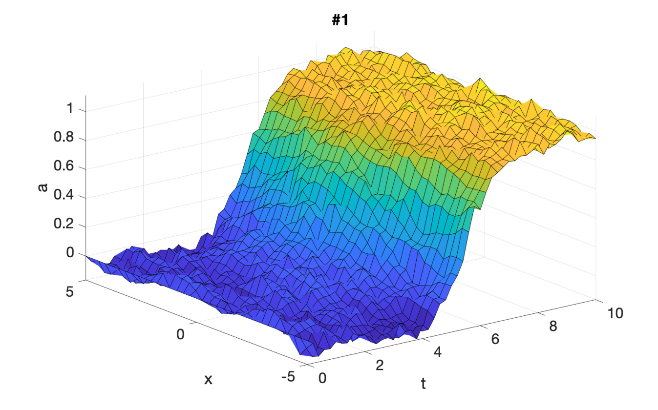
5 Transverse lattice
1 SPDE spatial lattice
Stochastic fields in an SPDE are stored in a cell array that can include one or more real or complex arrays, . Here is the internal field index, is a dimensional spatial lattice index for d space-time dimensions, and is the ensemble index. For a cell array of multiple fields, .., these must each have either the same number of points or one point per dimension. When specifying the spatial lattice, one must define:
- dimensions
-
The dimensionality in time and space. The default is an SDE: .
- points
-
The number of integration points. The first cell default points is . This can have a cell index if there are multiple field cells, provided the indices are compatible for broadcasting, eg , to allow different dimensions to be input. After the first or base cell dimension, the default is the previous cell dimension, with ones in the higher dimensions unless a value is already present in the previous cell.
- steps
-
The number of intermediate steps per plotted point. The default is . This is the same for all cells, and can modify any space-time dimension.
- ranges
-
The integration ranges in each dimension. The default is . This is the same for all cells.
- origins
-
The origins of the space-time integration domains. By default, the origin is for the time coordinate and for the space coordinates ( is the variable) such that the spatial grid is symmetric around .
There is a restriction, which is that the first cell must have the maximum number of points in each dimension.
The spatial points in the n-th dimension are at , so the spacing for points is . For periodic boundaries, the boundaries where fields and derivatives are equal are at and . For other boundary types, the boundary values are defined at the first and last points.
2 Field indices
In the functions , and , the field and noise variables and have extended dimensionality compared to the -dimensional case, to index the transverse lattice. The indices are , where the:
- field
-
index corresponds to the field index for and the noise index for .
- intermediate
-
indices which are absent in the -dimensional case, correspond to the spatial grid and have the same structure. For example, in the case with dimensions = 3, indicating one time index and two spatial dimension, corresponds to the two space indices.
- last
-
index corresponds to the stochastic trajectory.
For storing space coordinates like , the first and last index are . Where Fourier transforms are used internally, the momentum arrays have zero momentum as the first index to follow standard discrete Fourier transform conventions. This is changed to a symmetric convention in all stored graphics data outputs that are functions of momentum space.
3 Integrals and averages
There are functions available in xSPDE for spatial grid averages and integrals, to handle the spatial grid. These are Ave and Int, which are used to calculate observables for plotting. They operate in parallel over the lattice dimensions, by taking a vector or scalar quantity, for example a single field component, and returning an average or a space integral. In each case the first argument is the field, the second argument is a vector defining the type of operation, and the last argument is the parameter structure. If there are two arguments, the operation vector is replaced by its default value.
Int(o, [dx, ] p)
Integrates over the spatial grid to allow calculation of global quantities. To take an integral over the spatial grid, use the xSPDE function Int with arguments (o, [dx, ] p).
This function takes a scalar or vector quantity o, and returns a trapezoidal space integral over selected dimensions with vector measure dx. If an integral is taken over dimension j. Dimensions are labelled from j = 1,2,3 … as in all xSPDE standards. Time integrals are ignored at present. To integrate over an entire lattice, set dx = p.dx, which is the default value if dx is omitted, otherwise set dx(j) = p.dx(j) for selected dimensions j.
If momentum-space integrals are needed, first use the transforms switch to make sure that the field is Fourier transformed before being averaged, and always input dk instead of dx.
Warning: if dk is omitted, xSPDE assumes that you want to use the default of dx! This will generate incorrect results for momentum integrals.
Ave(o, [av, ] p)
Spatial grid averages can be used to obtain stochastic results with reduced sampling errors if the overall grid is homogeneous. An average is carried out using the built in xSPDE function Ave() with arguments (o, [av, ] p).
This takes a vector or scalar field or observable, defined on the lattice, and returns an average over the spatial lattice. The input is a field a or observable o, and an optional averaging switch av. If , an average is taken over dimension j. Space dimensions are labelled from j = 2,3… as elsewhere. If the av vector is omitted, the average is taken over all space directions.
6 Boundary conditions
1 Transverse boundary types
Transverse boundary conditions must be given for all partial differential equations. Common transverse boundary types are of three types: Neumann (specified derivative), periodic, or Dirichlet (specified field). These are obtained using , which is specified for each cell , space dimension , field index and boundary .
If boundaries are omitted for any dimension the default is , which gives periodic boundaries in that dimension for all field indices, and permits the use of Fourier transforms and an interaction picture as described above.
The value of is a matrix whose column index is the field index, and whose row index (j) is given by for the lower and upper boundary type respectively.
Spatial derivatives or other functions linking different spatial points can be specified either in the functionals , or else in the function, provided the derivative terms are linear functions of the fields. Use of the function allows an interaction picture algorithm, with increased efficiency. The function is available with all boundary conditions, but works best in periodic cases.
The default boundary conditions are periodic. The implicit setting of this is that periodicity is enforced such that , which is the usual discrete Fourier transform requirement.
Otherwise, the differential equation boundaries are specified at , , using the cell-array input , which is defined per field cell, space dimension (), field index () and boundary . Here is the transverse dimension, not including time, which only has an initial condition.
In summary the available boundary types are:
- Neumann:
-
For specified derivative boundaries,
- Periodic:
-
For periodic boundaries,
- Dirichlet:
-
For specified field boundaries,
These are specified in a cell array: sets the lower boundary type in dimension d for the i-th field component, while gives the upper boundary type. Each space dimension, variable and boundary is set independently. In xSPDE, the equations are always initial value problems in time, so the time dimension boundary specification for is not included.
Example: boundary types in a 2-dimensional PDE
Suppose there is one field cell with two field indices, and mixed boundaries in space: Dirichlet for a lower boundary at , and and Neumann for an upper boundary at , for the first field , with the opposite combination in the second field component, , hence
p.boundaries{2} = [1,-1;-1,1];
The field cell index is , which can be omitted here.
2 Transverse boundary values
For non-vanishing, specified boundary conditions, the boundary values can be entered either using , if they are constant in time, \or else, if they are dynamical, the function is specified. This returns the boundary values used for the fields or derivatives in a particular cell and dimension as an array of dimension , where .
Here is the current field cell array, is the field index, and is the space index, where is the index of the dimension whose boundary values are specified. For this dimension, only two values are needed: for the lower and upper boundary values, which could either be field values or their derivatives. An ensemble index is also needed if the boundary values are stochastic.
Boundary values can be a function of both the fields () and internal variables like the current time (). These may have stochastic initial values at which are calculated only once. In such cases the boundary values must first be initialized, so the routine is first internally initialized with time , and with random Gaussian values in the input field . These are delta-correlated in space, i.e., with the same definition as “inrandoms”. The xSDPE program stores the returned values for the boundaries in an internal cell array, , for later use if required.
The default boundary value is zero, if not specified.
3 Example: boundaries in a 2-dimensional PDE
Suppose there are two fields, and we wish to set boundary values.
We take boundary values as Dirichlet for and Neumann for in field variable 1, and Neumann for and Dirichlet for in field variable 2. Suppose the boundary values are different from the default values of , , so that:
| (12) |
These are set in the following code:
p.boundfun = @mybfun p.boundaries{2} = [1,-1;-1,1]; ... function b = mybfun(a,~,~,p) % b = mybfun(a,c,d,p) calculates boundary values b(1,2,:) = a(1,end,:); b(2,1,:) = -a(2,end,:); b(1,1,:) = 1+0*a(1,end,:); b(2,2,:) = -1+0*a(1,end,:); end
4 Transverse plots
A number of plots at equally spaced points in time can be generated through. For example, adding the line below creates 3 time-sliced plots at :
p.transverse{1} = 3;
7 Output transforms
For graphical output, Fourier transforms involve a sum over the lattice points using a discrete Fourier transform at the lattice points , so that:
| (13) |
The momenta have an interval of
| (14) |
with values given for even n by:
| (15) |
and for odd n by:
| (16) |
Once Fourier transformed, the function can be used to take any further functions or combinations of Fourier transformed fields prior to averaging. Important points to keep in mind are as follows:
- •
Fourier transforms are specified for the k-th observe function independently of all other functions, by specifying .
- •
Here is a logical switch, set to if the dimension requires a Fourier transform, and to if there is no Fourier transform.
- •
The internal fields are available for use in making functions of momentum for use with observations.
- •
In propagation calculations, the momentum lattice values start with , following standard Matlab and FFT conventions.
- •
For storing and graphing, momentum lattice values are reordered to start with , following standard graphics and mathematical conventions.
8 Initial random fields
When , an initial Gaussian random field is generated with delta-correlations in -space. This corresponds to a variance of for a lattice volume of for three space dimensions, and similarly for other cases.
When , an initial random field is generated with delta-correlations in -space. This can be filtered with a user-specified filter function to give , then inverse Fourier transformed to give . Both random fields are passed to the function as an extended vector , for field initialization in space.
When , an initial field of uniform random numbers is generated for jump processes.
These can all be specified as cells of multiple random fields, and passed to the initial function in the order of [randoms,krandoms,urandoms].
For multiple fields, one may combine random fields of different dimensionality using different cell-array indices. The “missing” dimension has only one point. This has a corresponding reduced lattice volume of , if the third dimension has only a single point for this field. If all space dimensions are missing, then .
There is a user specified filter function available, to modify random fields , that are delta-correlated in momentum space using a filter function, ’rfilter’ so that , before being used. The corresponding correlations are:
| (17) |
On a lattice, we replace the Dirac continuous delta-function by a discrete Kronecker delta function scaled by an inverse volume element either in space () or momentum () . The xSPDE Fourier transforms are given by a symmetric Fourier transform, so that if we inverse Fourier-transform the space inrandoms, without filtering, then:
| (18) |
These have random initial values that are real and delta-correlated in space, so that:
| (19) |
The corresponding noises in position space are correlated according to:
| (20) |
Similarly, if we don’t conjugate the k-noise, then:
| (21) |
However, if we define , then we obtain complex noise that is only delta correlated when conjugated.
| (22) |
This is obtainable with the x-space noise as well, but the utility of the k-space noise is that it can be filtered to have nonlocal correlations in space if required.
9 Noise fields
During propagation in time, noises are Gaussian noise fields delta-correlated in space-time. They are calculated in an analogous way, except with an additional factor of because they are delta correlated in time. They have a variance of . Reduced dimension cells with volume have a noise variance .
There is a user specified scaling function available, to take random knoises in momentum space that are then scaled using a filter function, ’nfilter’ so that , before being used:
| (23) |
When , an initial field of uniform random numbers is generated for jump processes.
All noises can all be specified as cells of multiple noise fields, and are passed to the deriv function in the order of [noises,knoises,unoises].
Chapter 4 SPDE theory
This chapter describes the basics of stochastic partial differential equation (SPDE) theory, in order to explain the background to the numerical methods.
1 SPDE definitions
A stochastic partial differential equation or SPDE is defined in both time and one or more space dimensions . We suppose there are total space-time dimensions. The space-time coordinate is denoted as .
The stochastic partial differential equation solved is written in differential form as
| (1) |
Here, is a real or complex vector field, is a vector function of fields and space and a matrix function. The new feature is that terms can now include the operator , which is a differential term in a real space . The exact structure of these terms is important, and not all such equations have well-behaved solutions [48, 49].
In many common cases, the noise term is delta-correlated in time and space:
| (2) |
One can also have noise with a finite correlation length defined by a noise correlation function in space so that:
| (3) |
It is even possible to have noise with a finite correlation time. Currently, these are not directly treated in xSPDE, although user definitions of this are possible by adding a customized noise function.
Additionally, the initial field has a probability distribution. In most examples, we suppose that this initial random field distribution can be generated as a function of Gaussian distributed initial random fields , where:
| (4) |
However, it is also possible that the initial random fields are also not delta-correlated, so that
| (5) |
Both finite correlation length and delta-correlated noise and random terms can be used in xSPDE simulations, with finite correlation lengths defined through a Fourier transform method.
2 Boundary conditions
There are three types of boundaries that are commonly used. They are specified independently for each space dimension , field component and lower or upper location . Each has a specific boundary type. These are described with a numerical code , as:
- Dirichlet
-
(specified value, ): .
- Periodic
-
(): .
- Robin/Neumann
-
(specified derivative, ): .
The coordinates are locations where boundary conditions are enforced. There are five types of boundary combinations of these for each dimension and field variable. Note that the boundary type can change the error stability properties of an equation.
Periodic boundaries can’t be combined with other types, as this defines both boundaries:
- a)
-
periodic-periodic- P-P: "0,0"
- b)
-
Dirichlet-Dirichlet- D-D: "1,1"
- c)
-
Robin-Robin- R-R: "-1,-1"
- d)
-
Robin-Dirichlet- R-D: "-1,1"
- e)
-
Dirichlet-Robin- D-R: "1,-1"
Just as with the derivative term, each of these types can change with dimension and field component. Specified field or derivative values can be any user-defined functions of space, time, and field amplitude or simply have fixed values. Currently, all combinations of boundaries can be treated in xSPDE.
3 Spatial grid and boundaries
The location of the boundary at is important in solving (S)PDEs, especially if high accuracy is required, or if field values at the boundary are needed.
Suppose the spatial grid spacing is and the number of grid points in a particular dimension is , then the maximum range from the first to last computed point is:
| (6) |
Noting that , and this means that the space-time points for an origin vector are at:
| (7) |
There are two slightly different spatial boundary locations used in xSPDE, depending on the type of boundary conditions specified, as follows:
1 Periodic boundary
For the default case of a periodic boundary, the logical boundary location is arbitrary. The indices are arranged as though on a circle from . It is useful to suppose the boundary is simultaneously at and at . Neither upper or lower logical ’boundary’ is at a grid point. The effective range of the domain is , due to this displaced boundary.
Only the values at points are computed, and one must regard the point where the periodicity is enforced as interpolating between the last and first point.
2 Non-periodic boundary
For the case of a non-periodic boundary, including Dirichlet, Robin and Neumann boundary conditions, the indices are in a line from . The lower and upper lower boundaries are at and at . In some PDE methods the logical boundaries are outside the grid boundaries, but that is not the case here. Unlike the periodic case, boundaries are enforced at the first and last point.
This is different to what is found in most trigonometric transform software, but this approach allows for a unified treatment of multiple types of algorithm. For finite difference derivatives at the boundaries, this leads to the usual result that the central difference approximation to the second derivative is of first order (in ) at the boundaries, while it is of second order elsewhere.
With spectral methods, the derivative boundaries are obtained with a combination of an interaction picture transform and additional polynomial terms. For simplicity, only linear, even order space derivatives are included in the linear propagator for the interaction picture (see 5), which means that other space derivatives must be included using finite differences.
4 Multidimensional walk
The simplest example of an SPDE is the multidimensional Wiener process:
| (8) |
This has a solution that is identical in appearance to an SDE:
| (9) |
Just as for an SDE, this means that the initial mean value does not change in time:
| (10) |
Since there are no spatial derivatives here, boundary values are not important. One can regard this as having periodic boundaries, which by the xSPDE conventions means that no boundary conditions are enforced - since periodic boundaries do not alter computed values when there are no derivatives.
1 Variance solution
The noise correlation is non-vanishing from Eq (2), so the variance must increase with time:
| (11) |
Integrating the temporal delta function gives unity. The spatial delta-function is replaced by in a discretized lattice calculation at points with cell volume , which means that the second moment and the variance both increase linearly with time:
| (12) |
The probability on the lattice for observing lattice field values follows an elementary diffusion equation:
| (13) |
which is an example of Eq (27). From this equation and using Eq (29), the first two corresponding moment equations in this case are
| (14) |
These differential equations are satisfied by the solutions obtained directly from the stochastic equations, but as one can see, the coupling between the lattice points provides more interesting behavior. This requires derivative terms such as Laplacians.
5 Interaction picture
To treat Laplacians, spectral or interaction-picture methods can be very efficient, with much lower errors and much faster run-times. This is because they do not have the stability problems of finite difference methods when treating higher-order derivatives, which allows much larger time-steps to be used.
To explain the interaction picture algorithm, SPDEs often contain terms which are linear in the field variables , including derivative operators acting on . This can be treated exactly using an interaction picture, which leads to dramatically reduced time-step errors and higher stability [50, 30], by using a spectral method to compute derivatives. These methods are also very useful in non-stochastic PDEs.
In summary, the interaction picture provides a means to solve for linear space-derivative terms in the propagation in an efficient way. This is based on introducing local variables for the field variables . It is convenient for the purposes of describing such interaction picture methods to introduce an abbreviated notation as:
| (15) |
Hence, we can write the differential equation as:
| (16) |
Here should include the highest order derivatives, as these have the largest eigenvalues, but lower-order derivative terms may occur in the other terms.
1 Linear propagator
Next, we define a linear propagator. This is given formally by:
| (17) |
where , is the interaction picture origin, and the notation includes setting boundary values. Transforming the field to an interaction picture is achieved on defining:
| (18) |
As a result, the equation of motion is:
| (19) |
This allows an SPDE to be treated with transformations using Fourier or discrete sine/cosine transforms. Our implementation uses a diagonal linear operator L without space-dependence. The linear operator can have any derivative in the periodic case, but only even order derivatives in the Dirichlet and Neumann case.
As well as the linear term, derivatives and nonlinear functions that are not tractable with spectral methods can appear in the residual term , where they are treated using finite difference techniques. As a result, while the interaction picture does not handle all possible derivative terms, it also does not restrict them from being used elsewhere in the equations.
Other methods exist in the literature. Improved convergence properties are obtained for some problems in a spectral picture using an exact solution of a linear part of the drift term [51, 52], or stochastic noise terms [53], as well as the Laplacian terms. The xSPDE code has user-definable functions that can be adapted to include these.
6 Fourier transforms
It is often useful to transform a field to implement the interaction picture, or to extract nonlocal correlation properties in space. The Fourier transforms or spectrum definitions used in xSPDE are given by the symmetric Fourier transform definition:
| (20) |
The inverse Fourier transform is the function:
| (21) |
In simulations, this is not combined with any time (or space) averaging as in the temporal Fourier transforms. The reason for this is that the interaction picture transformations must be invertible, which is the case for a point-based discrete Fourier transform.
1 Normalization
During propagation, we define temporary internal fields , that are normalized using FFT conventions:
| (22) |
Otherwise, for graphical and output averages, we define Fourier transforms using physics and mathematics conventions:
| (23) |
Note that this rescaling is consistent, because
| (24) |
7 Trigonometric transforms
Taking the interaction picture approach, we now consider other types of boundary conditions, which we initially assume here are either a zero field (Dirichlet) or a zero derivative (Neumann). We will only treat cases of even order derivatives, which do not change the trigonometric function. Any odd order derivatives are taken to be included in the finite difference () term.
1 Zero boundary cases
In the spectral transform method in one space dimension, with zero boundaries, one uses a trigonometric function, to expand as:
| (25) |
The discrete inverse transform allows evaluation at sample points , in order to satisfy the boundary conditions:
| (26) |
The trigonometrical function is defined such that:
| (27) |
The propagated equation is exactly soluble for the sampled points, since for each component
| (28) |
Hence,
| (29) |
This is an exact solution, provided the initial condition has the given expansion. This of course is usually an approximation itself, which should be checked by changing the grid. There are no other approximations made on the transverse derivative. Provided the values are the same, this propagator is identical for all types of trigonometric and Fourier transforms.
As explained in (2), there are five boundary combinations that are possible in each dimension and field component. Each has a corresponding xSPDE boundary type and spectral integrator. Each boundary type is specified to depend on the space dimension and the field component, as well as having boundary values depending on time and any field value.
Currently, all can be treated in xSPDE using finite differences, and each type of boundary also has a spectral method that preserves the boundary requirement. In principle one can define the trigonometric transforms to correspond to whole symmetries whose boundary is at a grid point, as used in xSPDE, or half symmetries which are half-way between two grid points.
All spectral methods used in xSPDE make use of boundaries at a grid point, in order to compute the relevant terms, which means that there is greater compatibility with the finite difference methods, when the boundaries are at the grid points. Differential equations can also have first order terms, which currently require using either finite differences or periodic boundaries.
It is possible to compute first-order derivatives with spectral methods, but these turn sine transforms into cosine transforms. This is not compatible with trigonometric interaction picture transformations used in XSPDE. As a result, any odd-order derivative terms must be computed using finite differences in all cases , except for the periodic case, where either method can be used.
In summary, spectral transforms can all be implemented using fast FTT, discrete sine (DST) or cosine (DCT) transforms. The spectral method used is specific to the boundary type. The definitions used here correspond to the standard definitions [54, 55], except for one-based indexing, normalization, and extra points at the boundaries, explained below.
2 Finite boundary values
For the case of finite boundaries, a combination of trigonometric and polynomial functions are used to expand the fields, so that:
| (30) |
Here, the functions are inhomogeneous polynomial terms specified to satisfy the non-vanishing boundary conditions such that:
| (31) |
while the trigonometric expansion simply has to satisfy the equation with zero boundaries.
8 Transforms and boundaries
For Dirichlet or Neumann/Robin boundaries, the following expansion can be employed in each dimension. We only describe one space dimension for simplicity with:
| (32) |
where are chosen to satisfy the initial and boundary conditions. Boundaries are taken, for the purposes of explanation, as being from to . This is not the case in the actual code, which can treat arbitrary boundary locations due to the use of the optional origins input to change the origin.
Unlike fast Fourier transform (FFT) definitions, there are multiple distinct trigonometric transforms . These are generally labeled DST-(n) and DCT-(n), where . They correspond to distinct boundary combinations, as explained below.
Suppose there are computational grid-points. For the spatial grid (1-based), this corresponds to , with , so we have and , as elsewhere in the manual.
In carrying out a discrete transform on points, with standard trigonometric transform definitions of , there are less transform grid points required if some boundary values are defined due to Dirichlet boundaries, hence . This is because xSPDE stores the full computational range, , with boundary values.
Sometimes one may wish to refer to the corresponding periodic Fourier transform size, . This is , except for DST-I , when it is .
An unnormalized inverse gives the original array multiplied by , where is the periodic size, so our definitions include a normalization of . Here , the number of points in the standard DST/DCT definitions, differs from both the xSPDE computation grid size that includes both boundaries, and also from the periodic size, which always includes one (periodic) boundary.
Our notation is based on standard discrete sine and cosine transform definitions. Here we use based indices throughout. For all coordinates, including these examples of discrete Fourier transforms, with an origin at and an integration range of , we define:
| (33) |
If we regard the transforms as having arguments of form , the momentum spacings given below are such that:
| (34) |
The internal momentum definitions used in the propagator calculations are therefore different to those used in external graphs and in periodic boundary cases.
The following lists the trigonometric transforms required to obtain the transform from , and vice-versa, for the four non-periodic boundary types in each dimension and field index.
1 D-D case: Discrete map (DST-I)
Let , and . The discrete representation of is:
Forward transform: DST-I
| (35) |
Inverse transform: DST-I (36)
The forward transform does not require the values at the end-points of and , which are set to zero in this case. This is implicit in the sine expansion, since (n. Second derivatives are proportional to .
2 R-R case: Discrete map (DCT-I)
Let , and . The discrete representation of is:
Forward transform: DCT-I
| (37) |
Inverse transform: DCT-I
| (38) |
The forward transform requires the values at the end-points of and , which are not zero in this case. It is equal (up to a factor) to a discrete Fourier transform of real numbers with even symmetry about and . As a result, the equivalent discrete derivatives at both the end-points are zero. Second derivatives are proportional to .
3 D-R case: Discrete map (DST-II/III)
Let , and . The discrete representation of is:
Forward transform: DST-III
| (39) |
Inverse transform: DST-II
| (40) |
The forward transform does not require the value at , which is zero in this case. This is implicit in the sine expansion, since (n. This transform implies a boundary condition that is odd around , and even around . Second derivatives are proportional to .
4 R-D case Discrete map (DCT-II/III)
Take . The discrete representation of is:
Forward transform: DCT-III
| (41) |
Inverse transform: DCT-II
| (42) |
The forward transform does not require the value at , which is zero in this case. This transform implies a boundary condition that is even around , and odd around . Second derivatives are proportional to .
9 Frequency or momentum grid
The frequency or momentum grid spacing is defined for all output graphs and periodic Fourier transforms as
| (43) |
The internal momentum grid spacing used can differ from this, depending on the transforms used in the interaction picture. As explained above in Section (8), the internal momenta for trigonometric transforms are:
| (44) |
This is because the xSPDE algorithms allow the use of a sequence of interaction pictures. Each successive interaction picture is referenced to , for the n-th step starting at , so . It is also possible to solve stochastic partial differential equations in xSPDE using explicit derivatives, but this is less efficient.
A discrete Fourier transform (DFT) using a fast Fourier transform method is employed for the interaction picture (IP) transforms used with periodic boundaries. This is normalized differently to the graphed Fourier transforms, but the difference is not computationally significant. However, the used internally changes with the precise type of trigonometric transform used in other cases.
In one dimension, the DFT is usually defined by a sum over indices starting with zero, rather than the Matlab convention of one. Hence, if :
| (45) |
For periodic boundaries, the IP Fourier transform can be written in terms of an FFT as
| (46) |
The inverse FFT Fourier transforms divide by the correct factors of to ensure invertibility. Due to the periodicity of the exponential function, negative momenta are obtained if we consider an ordered lattice such that:
| (47) |
This Fourier transform is then multiplied by the appropriate factor to propagate in the interaction picture, then an inverse Fourier transform is applied. While it is not scaled for interaction picture transforms, an additional scaling factor is applied to obtain transformed fields in any averages for output plots.
In other words, in the averages
| (48) |
where the indexing change indicates that graphed momenta are stored from negative to positive values. For plotted frequency spectra a positive sign is used in the frequency exponent of the transform to frequency space, to agree with common physics conventions.
10 Derivatives
1 Spectral derivatives
For spectral derivatives in the interaction picture, we define to obtain a derivative. To explain, one integrates by parts:
| (49) |
This means, for example, that to calculate a one dimensional space derivative in a Fourier interaction picture routine, one uses:
| (50) |
Here Dx is an array of momenta in cyclic order in dimension as defined above, suitable for an FFT calculation. The imaginary is not needed to give the correct sign, as it is included in the derivative array. In two dimensions, a full two-dimensional Laplacian is:
| (51) |
Then, on inverting the transform
| (52) |
2 Finite difference derivatives
For calculating derivatives using finite differences, the following central differencing method is used, away from the boundaries:
| (53) |
This raises the question of how to calculate derivatives at the boundary, for example at the lower boundary , where is not known, and similarly at the upper boundary. The answer depends on the boundary type [56], and is obtained by extending the boundary to additional points and that are assumed to extend the boundary condition:
Periodic:
| (54) |
Dirichlet: specified:
| (55) |
Robin/Neumann: specified:
| (56) |
In all cases the boundary value is evaluated as part of the derivative evaluation, so it can be a nonlinear function of .
Chapter 5 SPDE examples
1 Gaussian diffraction
Free diffraction and absorption of a Gaussian wave-function in space dimensions, is given by the partial differential equation (PDE):
| (1) |
The corresponding stochastic partial differential equation (SPDE) includes additional noise, so that:
| (2) |
The xSPDE spectral definition in space is:
| (3) |
Together with the initial condition that , this has an exact solution for the diffracted intensity with , in either ordinary space or momentum space:
| (4) |
Exercises
- •
Simulate Gaussian diffraction in three dimensions using an xSPDE function
- •
Check your results against the exact solution
- •
The example below stores data in a standard Matlab file.
function [e] = Gaussian() p.dimensions = 4; p.name = ’Gaussian diffraction’; p.initial = @(v,p) exp(-0.5*(p.x.^2+p.y.^2+p.z.^2)); p.linear = @(p) 1i*0.05*(p.Dx.^2+p.Dy.^2+p.Dz.^2); p.observe = @(a,p) a.*conj(a); p.olabels = ’|a(t,x)|^2’; p.file = ’Gaussian.mat’; p.images = 4; e = xsim(p); xgraph(p.file); end
- •
Add an additive complex noise of ) to the Gaussian differential equation, then replot with an average over samples.
- •
Work out the exact solution and repeat the comparisons.
Note that for this, you’ll need to add:
2 Stochastic Ginzburg-Landau equation
Including two space dimensions, or space-time dimensions of , an example of a SPDE is the stochastic Ginzburg-Landau equation. This describes symmetry breaking. The system develops a spontaneous phase which varies spatially as well. The model is used to describe lasers, magnetism, superconductivity, superfluidity and particle physics:
| (5) |
where
| (6) |
The following new ideas are introduced for this problem:
- 1.
is the space-time dimension.
- 2.
The ’dot’ notation used for parallel operations over lattices.
- 3.
is the linear operator - a Laplacian in these cases.
- 4.
produces movie-style images at discrete time slices.
- 5.
indicates a derivative operation, .
- 6.
is the default xSPDE coordinate range in space.
Exercises
- 1.
Solve the stochastic G-L equation for and .
- 2.
Change to a real diffusion so that .
In the first case, you should get the output graphed in Fig (1) .
clear; p.name = ’Extended laser gain equation’; p.noises = 2; p.dimensions = 3; p.steps = 10; p.linear = @(p) 1i*0.01*(p.Dx.^2+p.Dy.^2); p.observe = @(a,~) abs(a).^2; p.images = 6; p.olabels = ’|a|^2’; p.deriv = @(a,w,~) (1-abs(a(1,:).^2)).*a(1,:)+0.001*(w(1,:)+1i*w(2,:)); xspde(p)
Here the notation means that the operation is repeated over all values of the subsequent indices, which are the two spatial lattice indices in this case.
3 NLS soliton
The famous nonlinear Schrödinger equation (NLSE) is:
| (7) |
Together with the initial condition that , this has a soliton [57], an exact solution that doesn’t change in time:
| (8) |
The Fourier transform at is simply:
| (9) |
Exercises
- •
Solve the NLSE for a soliton using a function instead of a script, then include an additive complex noise of ) to the differential equation, and plot again with an average over samples.
4 Planar noise
The next example is growth of thermal noise of a two-component complex field in a plane, given by the equation
| (10) |
where is a delta-correlated complex noise vector field:
| (11) |
with the initial condition that the initial noise is delta-correlated in position space
| (12) |
where:
| (13) |
This has an exact solution for the noise intensity in either ordinary space or momentum space:
| (14) |
Here, the noise is delta-correlated, and , are the cartesian space and momentum space lattice cell volumes, respectively. Suppose that is the total number of spatial points, and there are points in the x(y)-direction, so then:
| (15) | |||||
In the simulations, two planar noise fields are propagated, one using delta-correlated noise, the other with noise transformed to momentum space to allow filtering. This allows use of finite correlation lengths when needed, by including a frequency filter function that is used to multiply the noise in Fourier-space. The Fourier-space noise variance is the square of the filter function.
The parameter indicates how many noise fields are generated, while indicates how many of these are spatially correlated, via Fourier transform, filter and inverse Fourier transform. These appear as additional noise cells. The filtered noises have a finite correlation length in general, but in this example are delta-correlated.
Exercises
- •
Solve the planar noise growth equation
function [e] = PlanarExample() p.name = ’Planar noise growth’; p.dimensions = 3; p.fields = 2; p.ranges = [1,5,5]; p.steps = 2; p.noises = 2; p.knoises = 2; p.inrandoms = 2; p.krandoms = 2; p.ensembles = [10,4,4]; p.initial = @Initial; p.deriv = @Da; p.linear = @(p) 0.5*1i*(p.Dx.^2+p.Dy.^2); p.observe = @(a,p) a(1,:).*conj(a(1,:)); p.olabels = ’<|a_1(x)|^2>’; p.compare = @(p) (1+p.t)/p.dv; p.images = 4; e = xspde(p); end function a0 = Initial(u,v,~) a0(1,:,:) = (u(1,:,:)+1i*u(2,:,:))/sqrt(2); a0(2,:,:) = (v(1,:,:)+1i*v(2,:,:))/sqrt(2); end function da = Da(~,w,z,~) da(1,:) = (w(1,:)+1i*w(2,:))/sqrt(2); da(2,:) = (z(1,:)+1i*z(2,:))/sqrt(2); end
- •
Add a decay rate of to the differential equation, then plot again
- •
Add growth and nonlinear saturation terms
5 Gross-Pitaevskii equation
The next example is a stochastic Gross-Pitaevskii (GP) equation [58] in two dimensions,
| (16) |
where is a correlated complex noise vector field:
| (17) |
with the initial condition that the initial random field and the noise are both filtered in momentum space
| (18) |
where:
| (19) |
We add a Gaussian filter in momentum space for both the initial random field and noise so that, if is a delta-correlated noise in momentum space:
| (20) |
This allows use of finite correlation lengths when needed, by including a frequency filter function that is used to multiply the noise in Fourier-space. The Fourier-space noise variance is the square of the filter function.
The first noise index, , indicates how many noise fields are generated that are delta-correlated in , while indicates how many of these are spatially correlated, via Fourier transform, filter and inverse Fourier transform. These appear to the user as additional noises, so the total is . The filtered noises have a finite correlation length.
Exercises
- •
Solve the stochastic GP equation (16), with a noise coefficient of , , and a stored output data file.
function [e] = GPE() p.name = ’GPE’; p.dimensions = 3; p.points = [101,64,64]; p.ranges = [1,20,20]; p.noises = 0; p.knoises = 2; p.inrandoms = 0; p.krandoms = 2; p.rfilter = @(w,p) w.*exp(-p.kx.^2-p.ky.^2); p.nfilter = @(v,p) v.*exp(-p.kx.^2-p.ky.^2); b = @(xi) .1*(xi(1,:,:)+1i*xi(2,:,:)); p.initial = @(u,v,p) (p.x+1i*p.y)./(1+10*(p.x.^2 +p.y.^2))+b(v); V = @(p) 0.01*(p.x.^2 + p.y.^2)-0.001*1i*(p.x.^2 +p.y.^2).^2; p.deriv = @(a,v,w,p) -1i*a.*(V(p)+conj(a).*a)+b(w); p.linear = @(p) 0.5*1i*(p.Dx.^2+p.Dy.^2); p.observe{1} = @(a,p) a.*conj(a); p.images = {2}; p.imagetype = {2}; p.olabels = {’|a|^2’}; p.file = ’GPE.mat’; e = xsim(p); xgraph(p.file,p); end
6 Characteristic equation
The next example is the characteristic equation for a traveling wave at constant velocity [59]. It is included to illustrate what happens at periodic boundaries, when Fourier-transform methods are used for propagation. There are a number of methods known to prevent this effect, including addition of absorbers - called apodization - at the boundaries. The equation is:
| (21) |
Together with the initial condition that , this has an exact solution that propagates at a constant velocity:
| (22) |
The time evolution at is simply:
| (23) |
Exercises
- •
Solve the characteristic equation given above, noting the effects of periodic boundaries.
function [e] = Characteristic() p.name = ’Characteristic’; p.dimensions = 2; p.initial = @(v,p) sech(2.*(p.x+2.5)); p.deriv = @(a,z,p) 0*a; p.linear = @(p) -p.Dx; p.olabels = {’a_1(x)’}; p.compare = @(p) sech(2.*(p.t-2.5)); e = xspde(p); end
- •
Recalculate with the opposite velocity, and a new exact solution.
7 Nonlinear Anderson localization
A random potential prevents normal wave-packet spreading in quantum-mechanics. This is Anderson localization [60]: a famous property of quantum mechanics in a random potential. A typical experimental method is to confine an ultra-cold Bose-Einstein condensate (BEC) in a trap, then release the BEC in a random external potential produced by a laser [61]. The expansion rate of the BEC is reduced by the Anderson localization due to the random potential. Physically, the observable quantity is the particle density , but there is a complication, which is that there are nonlinearities from atomic scattering [62].
This can be treated either using a Schrödinger equation with a random potential, at low density, or using the Gross-Pitaevskii (GP) equation to include atom-atom interactions at the mean field level. In this example of a problem where strong localization occurs, the general equations are:
| (24) |
In calculations, it is best to use a dimensionless form by rescaling coordinates and fields. A simple way to simulate this with xSPDE is to treat as a scaled field and to assume the random potential field as caused by interactions with second random field . This has the advantage that it is similar to the actual experiment and allows one to treat time-dependent potentials as well, if desired.
With the rescaling, this simplifies to:
| (25) |
A convenient initial condition is to use:
| (26) |
Exercise
- •
Solve Schrödinger’s equation without a random potential, to observe expansion.
- •
Include a random potential , to observe localization.
- •
Experiment with nonlinear terms and higher dimensions.
The GP equation is a mean field approximation; this is still not a full solution of the many-body problem! Also, the experiments are more complicated than this, and actually observe the momentum distribution.
8 Nonlinear Schrödinger equation with Neumann boundary conditions
This solves a (1+1)-dimensional PSDE with an initial condition of and
| (27) |
The solution is subject to Neumann boundary conditions with boundary values at zero
| (28) |
The equation is a deterministic nonlinear Schrödinger equation, which applies to nonlinear optics, Bose-Einstein condensates and plasma physics. The observables are and .
Notes
- •
The boundary conditions are specified with p.boundaries{2}, which is the x-dimension.
- •
The integration differential does not have to be entered, as this is the default.
- •
Three transverse graphs were specified, but they aren’t reproduced here.
- •
As there is only one field, which is the default, this does not need to be given.
- •
Since there is no noise, the default integration method was RK4.
function [e] = SolitonDerivN() p.dimensions = 2; p.points = [101,101]; p.ranges = [10,15]; p.initial = @(v,p) sech(p.x); p.observe{1} = @(a,p) a.*conj(a); p.observe{2} = @(a,p) Int(abs(D1(a,2,p)).^2,p); p.olabels = {’|a|^2’,’\int |da/dx|^2 dx’}; p.name = ’NLS soliton:spectral method + Neumann’; p.boundaries{2} = [-1,-1]; p.transverse = {3}; p.deriv = @(a,~,p) 1i*a.*(conj(a).*a); p.linear = @(p) 0.5*1i*(p.Dx.^2-1); e = xspde(p); end

Bottom figure: Evolution of the integrated modulus squared of the gradient for an NLS soliton with Neumann boundaries, showing how the reflected fields at the boundaries change the result even though this is not readily visible above.
9 Planar noise growth
This solves a (1+2)-dimensional PSDE describing the growth of noise in a planar vector field with a diffraction term giving rise to noise dispersion. The equation is:
| (29) |
The initial conditions are that , where:
| (30) |
the noise correlations are that , where:
| (31) |
The solution has periodic boundary conditions. The noise correlations for the second field are specified in momentum space. As there are no filters, the noise terms are delta-correlated in both momentum () and in space (). The exact results for comparison within each field are similar in position and momentum space:
| (32) |
Here, is the area of a lattice cell in space or momentum space. This is for the parameters used. The correlations are proportional to , the number of points in the spatial lattice, which is for the spatial lattice used:
| (33) |
Notes
- •
All three types of ensemble are used
- •
The much lower sampling error after integration is evident in the graphs
- •
Spatially resolved graphs show larger sampling errors
- •
The integration method is mid-point, as it is stochastic.
- •
Two k-space noises are specified, but they aren’t filtered.
- •
Under these conditions, x-space and k-space noise are identical.
function [e] = Planar()
p.name = ’Planar noise growth’;
p.dimensions = 3;
p.fields = 2;
p.ranges = [1,5,5];
p.points = 10;
p.noises = 2;
p.knoises = 2;
p.inrandoms = 2;
p.krandoms = 2;
p.ensembles = [10,2,12];
p.initial = @Initial;
p.deriv = @D_planar;
p.linear = @(p) 1i*0.5*(p.Dx.^2+p.Dy.^2);
p.observe{1} = @(a,p) Int(a(1,:).*conj(a(1,:)),p);
p.observe{2} = @(a,p) Int(a(2,:).*conj(a(2,:)),p.dk,p);
p.observe{3} = @(a,p) real(Ave(a(1,:).*conj(a(2,:)),p));
p.observe{4} = @(a,p) a(2,:).*conj(a(2,:));
p.transforms = {[0,0,0],[0,1,1],[0,1,1]};
p.olabels{1} = ’<\int|
a_1(x)|^2 d^2x>
’;
p.olabels{2} = ’<\int|
a_2(k)|^2 d^2k>
’;
p.olabels{3} = ’<< a_1(k) a^*_2(k)>>’;
p.olabels{4} = ’< |a_2(x)|^2>’;
p.compare{1} = @(p) (1+p.t)*p.nspace;
p.compare{2} = @(p) (1+p.t)*p.nspace;
p.compare{3} = @(p) 0.0;
e = xspde(p);
end
function a0 = Initial(u,v,~)
a0(1,:) = (u(1,:)+1i*u(2,:))/sqrt(2);
a0(2,:) = (v(1,:)+1i*v(2,:))/sqrt(2);
end
function da = D_planar(~,u,w,~)
%%Derivatives
da(1,:) = (u(1,:)+1i*u(2,:))/sqrt(2);
da(2,:) = (w(1,:)+1i*w(2,:))/sqrt(2);
end


10 Gross-Pitaevskii equation with vortex formation
This solves a (1+2)-dimensional PDE called the Gross-Pitaevskii equation. In addition to the standard GPE terms, it includes the vortex forming term . There is just one ensemble member, to demonstrate how a single trajectory can be imaged. The equation is:
| (34) |
Here, is the normalized derivative and indicates the two-dimensional cross-product. The system is initialized as
| (35) |
Notes
- •
This is a deterministic partial differential equation case
- •
The intermediate steps used are necessary to reduce integration errors
- •
The trap potential is an inline function, and is not a parameter
- •
Normalization is used because otherwise particle number is not conserved
- •
The output includes transverse images to show how the vortices develop
- •
Different imagetypes are used to show different 3D features
function [e] = GPEvortex2D() p.name = ’GPEvortex2D’; p.dimensions = 3; p.fields = 1; p.points = [50,40,40]; p.ranges = [15,16,16]; p.steps = 15; g = 200; om = 0.6; L = @(a,p) 1i*(p.x.*D1(a,3,p)-p.y.*D1(a,2,p)); V = @(p) 0.35*(p.x.^2+p.y.^2); p.initial = @(v,p) 0.1*exp(-V(p)); rho = @(a) g*conj(a).*a; p.deriv = @normda; p.da1 = @(a,w,p) -a.*(V(p)+rho(a))+om*L(a,p); p.linear = @(p) 0.5*(p.Dx.^2+p.Dy.^2); p.observe{1} = @(a,p) a(1,:).*conj(a(1,:)); p.observe{2} = @(a,p) a(1,:).*conj(a(1,:)); p.images = {2,2}; p.imagetype = {1,2}; p.olabels = {’|a|^2’,’|a|^2’}; e = xspde(p); function b = normda(a,w,p) % b = NORMDA(a,z,p) is a normalized derivative % Takes a derivative and returns a normalized step b = a+p.da1(a,w,p)*p.dtr; norm = sqrt(Int(abs(b).^2,p.dx,p)); b = (b./norm-a)/p.dtr; end end

11 Heat equation with non-periodic boundaries
This example solves a (1+1)-dimensional PDE with an initial condition of and
| (36) |
The solution is subject to either periodic boundary conditions or Dirichlet and/or Neumann with boundary values of zero at so that or . Each component has different combinations of boundary types. Using spectral methods the solutions here are exact, up to round-off errors of order , and are also much faster than with finite differences, which is demonstrated in the example.
In all cases the grid range is from to and the time duration is from to . In the examples, the spectral propagation error is reduced by more than and the time is reduced by a factor of compared to the finite-difference methods. The periodic method has boundaries just outside the grid.
Dirichlet-Dirichlet
With , the exact solution has the form:
| (37) |
Suppose that
| (38) |
and
For this case:
| (39) |
Neumann-Neumann
With , the exact solution has the form:
| (40) |
Suppose that
| (41) |
For this case:
| (42) |
Dirichlet-Neumann
Here , the exact solution has the form:
| (43) |
Suppose that
| (44) |
For this case:
| (45) |
Neumann-Dirichlet
Here , the general solution has the form:
| (46) |
Suppose that
| (47) |
For this case:
| (48) |
Periodic
Here , where accounts for the periodic boundaries being outside the grid range, so the general solution has the form:
| (49) |
Suppose that
| (50) |
For this case:
| (51) |
Notes
- •
This is a deterministic partial differential equation, although noise can be added
- •
Different boundary conditions apply to each component
- •
Sequential integration is used, but the initial condition is just recycled.
- •
In p1, the intermediate steps are necessary to reduce finite-difference errors
function [e] = Boundaries() p.dimensions = 2; p.points = [51,51]; p.order = 0; p.verbose = 1; p.method = @MP; p.fields = 5; p.ranges = [4,pi]; p.origins = [0,0]; p.initial = @heat_in; p.observe = {@(a,p) a(1,:),@(a,p) a(2,:),@(a,p) a(3,:)... @(a,p) a(4,:),@(a,p) a(5,:)}; p.compare = {@heat_1,@heat_2,@heat_3,@heat_4,@heat_5}; p.diffplot = {1,1,1,1,1}; p.olabels = {’a, DD’,’a, NN’,’a, DN’,’a, ND’,’a, PP’}; p.name = ’Heat test, spectral’; p.boundaries{2}= [1,1;-1,-1;1,-1;-1,1;0,0]; p1 = p; p.linear = @(p) p.Dx.^2; p1.deriv = @(a,w,p) D2(a,2,p); p1.steps = 40; p1.transfer = @(~,~,p) heat_in(0,p); p1.name = ’Heat test, finite diffs’; e = xspde({p,p1}); end function a = heat_in(~,p) a(1,:) = 4*sin(p.x)+sin(2*p.x); a(2,:) = 5+4*cos(p.x)+cos(2*p.x); a(3,:) = 4*sin(p.x/2)+sin(3*p.x/2); a(4,:) = 4*cos(p.x/2)+cos(3*p.x/2); a(5,:) = 2+cos(2*p.x/1.02)+sin(4*p.x/1.02); end function o = heat_1(p) o = 4*sin(p.x).*exp(-p.t)+sin(2*p.x).*exp(-4*p.t); end function o = heat_2(p) o = 5+4*cos(p.x).*exp(-p.t)+cos(2*p.x).*exp(-4*p.t); end function o = heat_3(p) o = 4*sin(p.x/2).*exp(-p.t/4)+sin(3*p.x/ 2).*exp(-9*p.t/4); end function o = heat_4(p) o = 4*cos(p.x/2).*exp(-p.t/4)+cos(3*p.x/2).*exp(-9*p.t/4); end function o = heat_5(p) o = 2+cos(2*p.x/1.02).*exp(-4*p.t/1.02^2)+... sin(4*p.x/1.02).*exp(-16*p.t/1.02^2); end


12 Peregrine solitary wave with arbitrary boundary conditions
Peregrine solitary waves are models for isolated large ocean waves. They are modeled as solutions to a (1+1)-dimensional PDE,
| (52) |
The Peregrine solution on an infinite domain is:
| (53) |
In the example, this is solved using finite boundary conditions, with initial values and boundary values that correspond to the exact solution.
Notes
- •
The boundary conditions are specified with p.boundaries{2}, which is the x-dimension.
- •
Four different boundary conditions are specified for a four component field.
- •
Spectral methods are used for accuracy
- •
No noise is included in the example below, but it can be added
- •
The boundary values are time-dependent, and are specified with p.boundfun
- •
For improved stability, the integration method is the semi-implicit MP method.
Errors
The reported errors in this example are reduced using second order extrapolation, by specifying p.order =2. This gives the following RMS average errors for the output intensity, averaged over all four cases:
- •
Step=0.000621
- •
Diff=0.00019
The ’Step’ error is from subtracting the most accurate results from lower accuracy results. With extrapolation specified, the most accurate results are the extrapolated results. The less accurate ones are at half the specified time-step. This is averaged over all space-time points, and normalized by the maximum intensity of .
The ’Diff’ error is from comparing the most accurate results with the analytic solution. This demonstrates a typical case where the time-step error is an upper bound to the true error. The maximum error occurs at large times, and is greater than the RMS error by about in this case. All four boundary types used give similar results and errors.
function e = Peregrine() % e = Peregrine() tests xSPDE for a nonlinear Schrodinger equn. % Using NN,DD,DN,ND boundary values with a spectral method % Uses time dependent boundary values for a peregrine solution p.dimensions = 2; p.noises = 1; p.fields = 4; p.order = 2; p.ranges = [10,10]; p.origins = [-5,-5]; p.points = [51,161]; p.method = @MP; p.olabels = {’|a|^2 , DD’,’|a|^2 , NN’,’|a|^2 , DN’,’|a|^2 , ND’}; p.boundaries{2} = [1,1;-1,-1;1,-1;-1,1]; p.boundfun = @boundval; sol = @(p) abs(per(p.x,p.t).^2); p.initial = @(~,p) per(p.x,p.origins(1))+zeros(4,1,1); p.compare = {@(p) sol(p),@(p) sol(p),@(p) sol(p),@(p) sol(p)}; p.observe = {@(a,p) a(1,:),@(a,p) a(2,:),... @(a,p) a(3,:),@(a,p) a(4,:)}; p.output = {@(o,p) abs(o{1}).^2,@(o,p) abs(o{2}).^2,... @(o,p) abs(o{3}).^2,@(o,p) abs(o{4}).^2}; p.name = ’Peregrine solution’; p.steps = 20; p.deriv = @(a,w,p) 1i*a.*((conj(a).*a)); p.linear = @(p) 0.5*1i*p.Dx.^2; e = xspde(p); end function [p,varargout] = per(x,t) % Generates peregrine solutions with alpha = 1/2, beta = A0 = 1 p = exp(1i*t).*(4*(1+2*1i*t)./(1+4.*(t.^2+x.^2))-1); if nargout == 2 dp = -8*x.*exp(1i*t).*(4*(1+2*1i*t)./(1+4.*(t.^2+x.^2)).^2); varargout{1} = dp; end end function bound = boundval(~,~,~,p) % Generates nonzero, time dependent boundary values [p,dp] = per(p.origins(2),p.t); bound = {p,p;dp,-dp;p,-dp;dp,p}; end

Bottom figure: Peregrine solution with Neumann-Neumann boundaries at
Part 4 Quantum phase-space
Chapter 6 Phase-space toolbox
This chapter describes how to use the xSPDE numerical toolbox to solve network and quantum dynamical problems in phase-space. For theoretical background, see Chapter (7). For detailed examples, see Chapter (8).
1 Quantum phase-space
Initially developed in the first half of 20th century, phase-space representations of quantum mechanics have been extensively developed, and utilized to simulate large bosonic Hilbert spaces, as well as small ones. Multiple such methods exist, including the classical Wigner [63], Husimi Q and Glauber-Sudarshan [64, 65] P representations, as well as the non-classical positive-P [66] and gauge-P [67] methods. If the reader is unfamiliar with these methods, they are referred to the theory sections in Chapter 7 and the original literature to obtain further explanations of these methods.
These different approaches have areas of applicability that depend on the Hilbert space dimension, as explained below.
1 Phase-space methods
This is used for phase-space mappings. Details are:
- p.phase = 1
-
- for a normally-ordered P or positive-P representation.
- p.phase = 2
-
- for a symmetrically-ordered Wigner-representation.
- p.phase = 3
-
- for an anti-normally-ordered Q-representation.
2 Laser amplification noise
Laser quantum noise is commonly modeled [68, 69, 70] using SDEs in a normally ordered quantum phase-space representation. Consider a model for the quantum noise of a single mode laser as it turns on, near threshold:
| (1) |
where the noise is complex, , so that:
| (2) |
Here the coefficient describes the quantum noise of the laser, and is inversely proportional to the equilibrium photon number.
As an example, try the following:
- •
Solve for the case of ,
using xSPDE input is:
clear
p.noises = 2;
p.observe = @(a,p) abs(a).^2;
p.olabels = ’|a|^2’;
p.deriv = @(a,w,p) 0.25*a + 0.01*(w(1)+1i*w(2));
xspde(p);
This input script can either be copied into a new script, or simply pasted into the Command Window, noting that one should usually type clear first when starting new interactive simulations. Most lasers have many photons and hence much less noise than this. At this small gain, numerical errors are negligible, so the program reports only small RMS average errors:
- •
Errors: Step=0.000621 Samp=0 Diff=0 Chisq/k=0
For larger gain, error-bars will display on the graph. These are calculated from the difference between using steps of size and steps of size . They only appear if greater than a minimum relative size, typically of the graph size, which can be set by the user. Here the time-step errors are too small to be graphed, there is no sampling error because only one trajectory is requested, and there is neither difference nor error, since there are no comparisons specified.
Note that specifying p.phase = 1 is not required, even though the phase-space is normally-ordered, which is the default phase-space method. This is because there is no vacuum noise in this classical noise case, and only the simple Glauber-Sudarshan P-representation is needed. Non-classical states require a positive P-representation.
3 Input parameters
More complex input parameters are stored in a structure which is input to the program. This is a superset of the parameters already defined. In the definitions below, the structure name is omitted, but we use in the examples.
While the quantum monte-carlo and phase-space toolboxes have some common parameters, they are distinct toolboxes that correspond to different Hilbert space bases. One must choose one or the other by either setting or . The defaults used are given in the phasepreferences function.
Common parameters with the standard SDE and SPDE simulations include ensembles, noises, inrandoms, points, steps, ranges. All have default values, but other choices can be input to over-ride the default values.
1 Phase-space parameters
Phase-space simulations can be initiated with a set of parameters that generate a default initial function. This is suitable for network simulations with gaussian inputs of squeezed and thermalized states.
- dimension
-
is for the type of calculation. For network transformations, dimension = 0.
- sqz
-
is the initial squeezing parameter vector, , per mode.
- alpha
-
is the initial coherent amplitude vector per mode.
- matrix
-
is a matrix transformation function used to create network transformations.
- tr
-
is an amplitude transmission vector used to attenuate the initial state.
- thermal
-
is a thermal fraction vector used to initialize a thermalized squeezed state.
- initial
-
functions initialise the equations. If omitted, the initial conditions are defined using the parameters above.
4 Gaussian boson sampling outputs
If one is interested in computing output probabilities for Gaussian boson sampling (GBS) photonic quantum networks, observe functions are available for comparisons with either experimental data, or exactly known test cases.
As every experimental group treats its data differently, xSPDE4 does not attempt to provide universal code for extracting and binning experimental data. This will be provided in a seperate codepackage. Instead, xSPDE4 focuses on simulating such networks in phase-space.
If p.dimension=0, where the mode index can be large, the mode index is treated as a space index rather than a line index. This aids in graphical rendering with xGRAPH.
1 Observe functions
The main observe functions correspond to binned photon-counting probability
distributions and marginal moments of various operator observables.
A summary, and brief description of the current list is given below:
| Label | Return type | Description |
|---|---|---|
| x | vector | -quadrature per channel |
| x2 | vector | -quadrature squared per channel |
| p | vector | -quadrature per channel |
| p2 | vector | -quadrature squared per channel |
| pn | vector | Output photon number, , per channel |
| nm | vector | Output photon number correlation in sequence |
| k | vector | Clicks per channel |
| km | vector | Click correlation in sequence |
| km2 | vector | Click correlation over two channels |
| km3 | vector | Click correlation over three channels |
| kmsub | vector | Subset of click correlations per CO channels |
| k1 | vector | Binned click probability - single partition |
| n1 | vector | Binned photon number probability - single partition |
| kn | array | Binned click probability - -fold partition |
| nn | array | Binned photon number probability - -fold partition |
2 Compare functions
The compare function is used for testing and for experimental data. The comparisons may include error data. This generates comparison plots, as well as error totals that are converted into a - error estimate when there are statistical variances.
Standard compare functions given below are analogous to their observe counterparts above, with compare functions denoted by the c at the end of each label. Generally, such test cases are only applicable when the output is unchanged from the input apart from a transmission factor , and when the input is a thermalised or pure squeezed state. For photon-number resolving (PNR) detector comparisons, uniform squeezing parameters are required for the inputs.
Functions labeled with an asterisk can be used with Gaussian states
having a coherent component :
| Label | Return type | Description |
|---|---|---|
| xc | vector | -quadrature per channel |
| x2c | vector | -quadrature squared per channel |
| pc | vector | -quadrature per channel |
| p2c | vector | -quadrature squared per channel |
| ∗pnc | vector | Output photon number, , per channel |
| nmc | vector | Output photon number correlation in sequence |
| kc | vector | Clicks per channel |
| kmc | vector | Click correlation in sequence |
| km2c | vector | Click correlation over two channels |
| km3c | vector | Click correlation over three channels |
| kmsubc | vector | Subset of click correlations per CO channels |
| k1c | vector | Binned click probability - single partition |
| n1thc | vector | Thermal input photon number probability - single partition |
| n1lsc | vector | Pure squeezed input photon number probability - single partition |
| knc | array | Binned click probability - -fold partition |
| nnthc | array | Thermal input photon number probability - -fold partition |
5 Sampling methods in phase-space
Generating initial samples of a phase-space distribution is the first step of any phase-space simulation, be that dynamical or input-output, such as for GBS. In most cases, analytical forms of the initial samples exist, which are straightforard to implement numerically.
The section outlines the sampling methods used to simulate GBS input and output distributions in phase-space, and perform comparisons with either experimental data, or exact tests.
1 Input-output samples
Simulating dynamic and static quantum systems in phase-space follows the same, general procedure, at least initially. In dynamical applications, initial stochastic samples generated from some phase-space distribution. These can be from a default gaussian description of coherent, squeezed or thermal states, given by the alpha, sqz, thermal and tr parameters, or else from an initial function, which takes precedence over the gaussian parmeters.
To simulate quantum networks in phase-space, one must first generate initial stochastic samples. This is achieved using the -ordering scheme (see Subsection 5 for theory) as stochastic samples for any Gaussian input state in any representation are generated following:
| (3) |
where are real Gaussian noises and
| (4) |
are thermal squeezed state quadrature variances which are altered from the pure squeezed state definitions, (50) and (51).
For normally ordering, the input amplitudes are converted to outputs as
| (5) |
which follows from Eq.(39). However for non-normally ordered methods, additional vacuum noise arising from the reservoir modes must be included.
This is achieved using a hermitian decoherence matrix
| (6) |
with decomposition where is the matrix square root and is a diagonal, positive matrix. The output amplitudes when are then obtained as
| (7) |
where as these are a classical phase-space.
2 Grouped correlations computation: Threshold detectors
Grouped correlations, or grouped count probabilities (GCPs), are binned photon counting probability distributions that can be simulated in xSPDE4 for photon-counting set-ups using both photon-number resolving (PNR) or threshold detection. These are defined analytically in Section 10, where all the nessecary background theory is presented in Section 6.
These observables are readily simulated in phase-space using the positive-P representation. For threshold detectors, one replaces normally ordered projection operator Eq.(61) with the positive-P observable
| (8) |
where is the output photon number.
The summation over exponentially many patterns implemented by GCPs (see Eq.(77) is simulated using a multidimensional inverse discrete Fourier transform
| (9) |
where and .
The Fourier transform removes all patterns which don’t contain counts, in doing this the Fourier transform simulates all possible correlations generated in a network. This reduces an otherwise computationally complex task into a highly efficient and scalable one, allowing comparisons to be performed on experimental correlations of any order.
3 Grouped correlations computation: PNR detectors
To simulate GCPs of PNR detectors, we are interested in the total number of output photons contained in each subset defined in operator form
| (10) |
As was the case for threshold detectors, we replace this total number operator with the phase-space observable
| (11) |
such that the actual GCP computation is performed as
| (12) |
We note that this method allows one to avoid the multi-dimensional Fourier transform needed for the threshold detector distribution. The Fourier transform has the effect of introducing Fourier overheads which can slow down simulations of multi-dimensional distributions, especially for dimensions .
Chapter 7 Quantum phase-space theory
This chapter describes the background of quantum phase-space theory, including dynamical problems obtained by transforming the master equation into a second-order partial differential equation called the Fokker-Planck equation (FPE), as well as input-output problems such as GBS.
1 Phase-space representations
Phase-space representations are an alternative description of quantum mechanics where one maps operators and fields of various orderings to classical probability distributions on a phase-space. This alternative description was first introduced by Wigner [63], and has since burgeoned into a vast field with applications to quantum optics, atom-optics, quantum information, and many more.
In this section, we introduce the phase-space representations implemented in xSPDE4, although one is not restricted to these representations. The outputs in phase-space are continuous real or complex variables whose stochastic moments are equal to quantum expectation values, including probability distributions obtained from experimental data such as photon counting experiments.
This assumes that the parameters are precisely known, and do not have noise or fluctuations. Even then, some differences from sampling errors due to finite numbers of experimental and theoretical counts.
For clarity, throughout this chapter, hats like are used to indicate operators that do not commute with each other, as opposed to stochastic variables like that do commute. For any given operator ordering, it is always possible to find a probability distribution such that the expectation of an operator product equals the stochastic variable correlations [71].
1 Glauber-Sudarshan P-representation
The -mode Glauber-Sudarshan P-representation expands the density matrix as a sum of diagonal coherent state projectors
| (1) |
where is a multimode coherent state eigenvector with corresponding eigenvalues . Coherent states [64] are the right eigenstate of the annihilation operator, , and are the most commonly used basis state to define phase-space representations, although other bases are possible, such as quadratures.
For classical states such as coherent and thermal states, the P-distribution satisfies the mathematical requirements of a probability distribution: Real, positive, non-singular and normalizable with
| (2) |
The P-representation breaks down for certain quantum states, giving non-positive and singular distributions. This is due to the lack of off-diagonal coherent state amplitudes required to represent nonclassical superpositions.
2 Positive P-representation
Part of a family of generalized P-representations developed to extend the Glauber-Sudarshan P-representation to quantum states [66], the normally ordered positive P-representation always generates a non-singular and positive distribution for any quantum state. The trade-off is that it is non-unique, which can lead to growing sampling errors for nonlinear Hamiltonians.
In the positive P-representation, the density matrix is defined as an expansion over a multidimensional subspace of the complex plane:
| (3) |
where is the positive-P distribution over coherent state amplitudes satisfying the normalization condition
| (4) |
The projector
| (5) |
is responsible for the doubled classical phase-space dimension. This allows off-diagonal amplitudes to exist, such that are now independent, generating two pairs of complex amplitudes.
One can restrict the distribution to a classical phase-space with , in which case the diagonal P-representation is obtained as a special case of the positive P-representation via the substitution . As stated above, for non-classical states such as squeezed or Fock states, this will lead to the well known singular behavior of the distribution.
Moments of the positive-P distribution are equivalent to normally ordered operator moments
| (6) |
where denotes a quantum expectation value and is the positive-P average in the limit of an infinite ensemble of stochastic trajectories.
3 Wigner representation
Although the diagonal P-representation is unsuitable for simulating non-classical states, not all classical phase-space distributions suffer from the same limitations. The symmetrically ordered Wigner representation and anti-normally ordered Q-function both produce positive, well defined distributions for Gaussian quantum states such as squeezed states. Unfortunately, for non-Gaussian non-classical states such as Fock and Schrödinger cats states, the resulting Wigner distribution is negative, and hence not a probability distribution.
The negativity of the Wigner distribution for some states is why its commonly referred to as a quasi-probability, and for an -mode system is defined as the Fourier transform of the symmetrically ordered characteristic function such that
| (7) |
where Tr () is the matrix trace and is a complex vector. For hermitian operators such as the density operator, the Wigner distribution always exists as a real-valued function on phase-space. This isn’t the case for non-hermitian operators, in which case Wigner distribution becomes complex.
The Wigner representation is directly applicable to symmetrically ordered operator products. Symmetric ordering, denoted , is the average over all possible combinations of creation and annihilation operators, for example:
| (8) | ||||
| (9) |
Therefore, moments of the Wigner distribution correspond to symmetrically ordered operator moments
| (10) |
where is the Wigner ensemble average.
For applications to photon-counting experiments, the Wigner representation is suitable for simulating quadrature operators as measured by homodyne detectors, which are symmetrically ordered. The ordering requirement makes applications to normally-ordered detectors both cumbersome, as one must reorder all operators to normal order, for example:
| (11) |
as well as inaccurate. The additional term arises from the reordering, as the Wigner representation adds half a quantum of vacuum noise per mode, causing a rapid increase sampling errors. Hence, the Wigner representation is unsuitable for simulations of normally-ordered photon counting probabilities.
4 Q-function
The standard form of the anti-normally ordered, e.g. , -mode Q-function is
| (12) |
and, like the Wigner function, can be expressed as the Fourier transform of the anti-normally ordered characteristic function.
Unlike the Wigner distribution, the Q-function distribution is always positive for any classical or non-classical state but is only defined for anti-normally ordered operator products with moments being obtained as
| (13) |
where denotes a Q-distribution ensemble average.
Like the Wigner function, this ordering requirment means that for applications to normally-ordered photon counting experiments, or any normally-ordered measurement, operators must be reordered. This is readily illustrated using the standard bosonic commutation relations Eqs.(41), where anti-normal ordered expectation value is reordered to
| (14) |
Therefore, the Q-function adds an entire quantum of vacuum noise per mode, generating the largest increase in sampling errors of any phase-space representation when used to simulate a normally ordered measurement. This accumulation of vacuum noise for multimode linear photonic networks rapidly causes Q-function simulations to become inaccurate.
5 -ordering
The amount of vacuum noise added by each representation can be used to define the operator ordering parameter , where corresponds to normal ordering, symmetric ordering and anti-normal ordering.
From the ability to define a common ordering scheme arises the ability to define a -ordered phase-space distribution. Since the Wigner and Q-function distributions can be defined as convolutions of the positive P-representation, a -ordered representation is defined as:
| (15) |
Here, is a -ordered distribution, is the positive-P distribution and are used to denote the normal-ordered non-classical phase-space variables, whilst denote a classical phase-space which is valid for .
Operator moments for any ordering can now be obtained via
| (16) |
where, as above, is a -ordered ensemble average.
2 Dynamics in phase-space
The density matrix master equation is basic to quantum theory, particularly for open quantum systems, the theory of which will be treated in more detail in Chapter 10. The master equations of most interest in this chapter have the standard Lindblad form:
| (17) | ||||
Here, is the total super-operator for terms, is the reversible system Hamiltonian, are operators that couple the system to the dissipative reservoir, and is the decay rate. The dissipative operators can be further classified by type and mode index , including vector indices if needed.
Solving the master equation using orthogonal basis methods is impractical, as the master equation has a memory requirement that scales as for modes, where , and is the dimension of the Hilbert space of a single mode. As , the Hilbert space dimension grows exponentially, limiting orthogonal basis methods to small mode numbers as the memory and CPU time grows rapidly. Therefore, large quantum systems like linear photonic networks or quantum fields are inaccessible, apart from using various approximations like mean-field or tensor network methods. Although even tensor networks eventually succumb to computational limitations.
One possible way to treat such large quantum systems is via quantum phase-space expansions. These methods convert the master equation into a stochastic differential equation, which are often more scalable than other methods [72, 73]. There are trade-offs, and this often may require further approximations.
The advantage arises from the phase-space distribution being sampled using random sampling, where each sample in phase-space requires a polynomial amount of storage, typically growing linearly with the number of modes. From this sampling procedure, it is also usually relatively straightforward to estimate sampling errors.
This approach started when Schrödinger [74] pointed out that quantum oscillators can have classical equations. This was extended to other systems [63, 75, 64], especially including lasers and quantum optics [68, 70, 69, 2].
1 Operator mappings
To perform dynamical simulations of a quantum system requires first mapping the master equation into a second-order partial differential equation called a Fokker-Planck equation (FPE) (see Chapter 1 for a theoretical review of FPEs). To do this, one requires a mapping between operator products, such as , and partial derivatives of phase-space distributions, i.e. .
Using the -ordered notation, unified operator identities can be defined to perform this differential equation mapping as:
| (18) |
If the resulting differential equation obtained from this mapping has a second-order positive-definite form it is an FPE, which is equivalent to an SDE (see Chapter 1 for theoretical background on SDEs), or an SPDE for quantum fields [76]. The noise can be additive or multiplicative, depending on the problem. Although we have defined a unified mapping for any ordered phase-space representation, not all methods give stable FPE equations [67], such as the positive P-representation, which can suffer from boundary-term corrections [67, 77]. The Wigner representation meanwhile requires a truncation of larger than second-order derivatives if the Hamiltonian is nonlinear [78], hence simulations only approximate the system dynamics, although this can be accurate in some cases [78]. The FPE obtained from the Q-function on the other hand is no longer positive-definite, which is a requirement for FPEs.
The total noise includes internal quantum noise generated from the Hamiltonian term , as well as reservoir noise terms generated from the coupling to the reservoir operators, which is proportional to the damping rate . There is a similar behavior in classical systems, except that these correspond to a high-temperature limit, and in most cases only have external reservoir noise from thermal fluctuations.
3 Damped harmonic oscillator
As an example, take the driven quantum harmonic oscillator. This has the Hamiltonian
| (19) |
where is the driving amplitude, and the harmonic oscillator frequency. If damping is added, it obeys the master equation
| (20) |
where is the temperature reservoir occupation (see Chapter 10).
This leads to a random walk in a complex space [1, 2]:
| (21) |
where the noise is complex and . The correlations are
| (22) |
1 Wigner dynamics
In the undriven, zero temperature Wigner case with 1, , and in a rotating frame so that , using the mappings Eq.(18), the probability follows the Fokker-Planck equation:
| (23) |
which is an example of Eq.((27)). Ignoring terms that vanish or can be obtained from symmetry, the first corresponding moment equations in each of the real and imaginary directions are
| (24) |
The steady-state is therefore a Gaussian distribution with , and . One can use an initial condition of , with , in order to replicate the steady state, which is a Gaussian with and.
2 Internal spectrum
Neglecting any boundary terms, the equation in frequency space is:
| (25) |
For sufficiently long times, the solution in frequency space - where is the angular frequency - is therefore given by:
| (26) |
The expectation value of the noise spectrum, in the long time limit, is:
| (27) | |||||
This equation can also be used for some classical problems, which correspond to the high-temperature limit of .
4 Stochastic gauge expansion
In this approach, the density matrix is expanded as a weighted integral over coherent state projection operators:
| (28) |
Here, in the stochastic gauge method [67], , where are each -dimensional complex numbers, and is a real or complex weight. The operator basis is defined using un-normalized coherent states , so that:
| (29) |
There are standard identities available, namely:
| (30) |
The hermiticity of means that every has a conjugate of equal weight, so the integral is sampled in pairs and , corresponding to a sum over samples of the real part of :
| (31) |
Operator averages are obtained through defining a weighted average as the infinite ensemble limit of a sum of trajectories:
| (32) |
Here, for hermitian operators,
| (33) |
with the approximation of taking only a finite number of samples . For example, the quantum average particle number is obtained on taking a weighted average of :
| (34) |
Individual trajectory photon numbers can be negative, although their large- average is non-negative. These trajectories correspond to Schrodinger cat superpositions, causing mixtures of positive and negative ’effective’ photon numbers. Such behavior is impossible in the diagonal Glauber-Sudarshan representation, where for a probabilistic distribution, only classical photon statistics occur [79, 80].
5 Input-output spectra
The spectrum of an internal field variable is not the one that is usually measured. An important application of stochastic equations is therefore in calculating output, measured spectra of lasers, quantum optics, opto-mechanics and quantum circuits [70, 81]. These have the feature that the measured output spectrum may also include noise from reflected fields at the input/output ports. If the quantum noise term in the Heisenberg equations for a cavity operator is given by: then the corresponding operator input-output relations are .
In quantum phase-space for the case of the harmonic oscillator or similar systems, is the noise term in the Langevin equation. The output fields that are measured are given by:
| (35) |
Hence one must include in the spectrum both the internal mode variables and the noise terms themselves. Solving for the spectra, one obtains auxiliary fields with
| (36) | ||||
In summary, it is the output fields that are amplified and measured. Hence one must be able to compute the spectra of the output fields for experimental comparisons. These have the additional feature that they include the reservoir noise , evaluated at the same time as the field is evaluated, since the reservoir noise is the input here. In xSPDE these are called auxfields.
1 Steady-state result
Consider the example of the damped quantum harmonic oscillator in the Wigner representation case with , and . Over long time-scales, so that one is in the steady state, the solution for is that:
| (37) |
This gives the following expectation values:
| (38) |
These are the expectation values of the zero temperature quantum fluctuations in the input and output channels. This means that the harmonic oscillator in its ground state is in equilibrium with an external vacuum field reservoir, also in its ground state. However, the internal spectral correlations of the harmonic oscillator are modified by the coupling.
While this is a simple result, exactly the same general type of behavior occurs in more sophisticated cases. These may include many coupled modes with nonlinearities. Additional or auxiliary fields that depend both on noise terms and internal stochastic variables are required. The soluble case given above is a useful test case, and it is treated numerically later in the manual.
6 Linear photonic network theory
In some quantum systems, output observables are obtained not via dynamical processes, but after a simple linear transformation of a multi-mode density operator. In the case of linear photonic quantum computing networks such as GBS, the mode transformation is traditionally generated by a network of beam-splitters, phase shifters, and mirrors [82, 83], although other set-ups include fibre delay lines [84, 85].
These networks act as -mode interferometers which interfere input photon, generating large amounts of entanglement due to the exponential number of interference pathways available to photons. In the ideal lossless regime, the network itself is defined by an Haar random unitary matrix , such that output modes are linear combinations of each input mode:
| (39) |
where and are the input and output annihilation operators for modes , respectively.
Practically, photon loss in the network is commonplace, thus causing the matrix to be non-unitary. Therefore, lossy networks are denoted by the transmission matrix . These give a different transformation law, where:
| (40) |
Here, the operators are noise operators which are necessary to conserve the operator commutation relations
| (41) |
The noise operators are independent, commuting operators, who comprise inputs from the reservoirs that cause losses, where the reservoirs are all in a vacuum state.
The inclusion of the loss matrix conserves the unitarity of the network. Substituting Eq.(40) into Eq.(41) and and taking expectation values for a vacuum state input gives
| (42) |
Next, we can define a new matrix
| (43) |
This is hermitian, since , and so has a diagonal representation as , for some unitary matrix . We assume that the transmission matrix is lossy, so that is positive definite and is real, representing absorption rather than gain.
7 Quantum input states
The density operator transformed by linear network has input modes, where one can have or , in which case the remaining modes are vacuum inputs at unused ports. If each input mode is independent, is a product of input states.
Currently, xSPDE can only generate input squeezed states and thermal states as outlined below. Other inputs are possible, since the positive P-representation and Q-representation are complete, positive representations, and can be added through user customization.
For pure squeezed vacuum states, the input is defined as
| (44) |
where is a vector of squeezing parameters and
| (45) |
is the squeezed vacuum state with squeezing operator , which satisfies the unitarity condition . Here, we have assumed the squeezed state phase is zero.
1 Pure squeezed states
Pure squeezed states are the default type of squeezed state generated in xSPDE. Given each input mode is independent, one can use the well known single-mode squeezed state theory [86, 87], to derive the basic properties of pure squeezed states.
Using the relations
| (46) |
the mean input photon number per mode is defined as
| (47) |
while the mean input coherence per mode is
| (48) |
For pure squeezed states, the coherence and photon number are related via .
Squeezed states are minimum uncertainty states and are therefore defined entirely by their quadrature variances. From the quadrature operators
| (49) |
which obey the commutation relation , the normally ordered -quadrature variance is defined as
| (50) |
while the normally ordered -quadrature variance is
| (51) |
2 Thermal squeezed states
As stated above, xSPDE4 can currently simulate pure and thermalized squeezed states, as well as classical thermal state inputs into a photonic network. This is achieved using a model for thermal squeezed states which alters the multi-mode input coherence as , with being the thermalization component which is input to xSPDE as p.thermal, whilst keeping the input photon number unchanged. This allows one to interpolate between pure thermal, , and pure squeezed, , states.
Thermal states are classical states with fluctuations larger than the vacuum limit such that their quadrature variances are . In terms of Fock states, the thermal state density operator for the -th mode is the single-mode state
| (52) |
which gives the well known single-mode photon number distribution
| (53) |
Thermal states can be used to generate thermal squeezed states with initial occupation , which gives [88]:
| (54) |
In the thermalized case, the relationship between coherence and photon number is modified, since to eliminate one must use the relationship that
| (55) |
Therefore:
| (56) |
Using the above theory, thermalized squeezed states can also be used as a test for numerical simulations of photon counting observables, as one can define the threshold detector projection operators in terms of the photon number and coherence as explained below.
8 Photon counting
Although linear photonic networks are conceptually very simple, when employed as quantum computers they generate samples from an output distribution which corresponds to the -hard matrix permanent, Hafnian or Torontonian functions. Which type of matrix function is evalutated depends on the input states to the network, with Fock states corresponding to the permanent and squeezed states corresponding to either the Hafnian or Torontonian functions, where the difference between these distributions comes from the type of detector used.
Currently in xSPDE4, only Gaussian states are generated natively, hence we restrict our discussion here to Gaussian state photonic quantum computing networks such as GBS. When photon-number resolving (PNR) detectors are used, photon count patterns, which are our samples of the output distribution, correspond ot the Hafnian function, while the Torontonian requires threshold detectors that “click” for a photon detection event.
From standard photon counting theory, the projection operator for observing counts is denoted by [87]
| (57) |
where denotes normal ordering and is the output photon number and is the maximum observable count.
For PNR detectors, which can discriminate between photon numbers, each detector is defined by the above projector, with varying depending on experimental implementation. Output photon count patterns are denoted by the count vector , and the projection operator for a specific output pattern given as
| (58) |
The expectation value of this pattern projector corresponds to the Hafnian [89]
| (59) |
which is -hard to compute at large . Here, is the sub-matrix of formed from modes with detected counts and is a covariance matrix.
Threshold detectors saturate for more than one count at a detector. Therefore, outputs are binary with denoting a detection event, or click, even if multiple photons hit the same detector, and is no detection event. From Eq.(57), the click projection operator is obtained by summing over all counts such that
| (60) |
which gives the standard threshold detector projection operator
| (61) |
The projection operator for a count pattern output is then similarly defined as
| (62) |
where the expectation value corresponds to the Torontonian function [90]
| (63) |
where is the sub-matrix of with covariance matrix .
1 Exact output examples: Threshold detectors
For photon counting probabilities obtained through threshold detection, a variety of probabilities can be computed exactly.
Initially, we are interested in computing the probability of detecting no photons at the threshold detector output, i.e. . From Marian [88], the single-mode photon number probability is known exactly from the full distribution of a thermalized squeezed state, , such that
Substituting the thermal squeezed state modified photon number Eq.(54) the vacuum state detection event probability can be derived as
Hence, the click and no-click probabilities for thermalized squezed states can be computed exactly in the limit of an identity transmission matrix or in the case of a fully thermal state input with Haar random unitary matrix as:
| (64) |
2 Exact output examples: PNR detectors
For PNR detectors, the multi-mode photon counting distributions are known exactly for both pure squeezed states and thermal states. These exact distributions are only valid if one assumes each input state has equal squeezing parameters , which in turn causes the input mean photon number to be equal for each mode .
For thermal states, the single-mode photon counting distribution Eq.(53) is a geometric distribution, which becomes clear by defining the success probability as
| (65) |
such that
| (66) |
This single-mode theory can be extended for multiple thermal state inputs as the sum of a geometrically distributed random variable with success probability is the random variable
| (67) |
which is negative binomially distributed with and . The total photon number distribution is then defined as
| (68) |
where is the total, or binned, photon number. At large , the distribution is a Gaussian with mean and variance
| (69) |
For pure squeezed states transformed by a lossless unitary matrix, the probability of observing total photon counts from modes is [91, 92]:
| (70) |
This distribution is well known due to the distinct oscillations between even and odd photon count bins. Such oscillations arises due to the generation of squeezed photons in highly correlated pairs in a parametric down-conversion process. Therefore, only even numbers of photons are ever generated, as in clear from the squeezing operator in Eq.(45).
In the limit , the total photon counting distribution reduces to a Poisson distribution for the even counts [91]
although the full distribution is considered super-Poissonian, i.e. the variance is now larger than the mean. The lossless distribution can also be written in terms of success probabilities as
| (71) |
where is defined in Eq.(65).
For lossless linear networks, the total photon counting distribution is also known exactly and is defined as [84]
| (72) |
where is a uniform amplitude loss coffieicent, which is applied as and is related to intensity loss via , and is the Gauss hypergeometric function. The lossy distribution converges to the lossless distribution Eq.(71) when as .
When identical thermal or pure squeezed states are input into a optical linear, one can use the above exact distributions to compare phase-space simulated grouped count probabilities, which are explained below.
9 Intensity correlations
We now explain two types of measurable correlations: Glauber intensity correlations [64] and grouped correlations [93, 94], also referred to as a grouped count probabilities (GCPs).
Intensity correlation simulations can only be performed on photon number operator observables. Therefore, although they are valid for determining photon number probabilities in click experiments, they correspond directly to PNR detector outputs. Meanwhile GCPs are valid for both threshold and PNR detectors.
Glauber’s -th order intensity correlation is defined as [64]
| (73) |
where is the correlation order. Multi-mode Glauber correlations determine the probability of detecting photons at modes.
The normal ordering requirement causes all creation operators to the right and all annihilation operators to the left. For example, the second-order correlation
| (74) |
corresponds to detecting one photon at , and one at .
Upon reordering, one obtains
| (75) |
The first term describes non-local correlations, which is the interference of photons between modes (or practically, detectors), while the second term describes the photon intensity at each mode (or detector), which are termed local correlations.
If the mean number of photons is small, such that a detector will only ever observe one photon, the intensity correlation becomes a coincidence count
| (76) |
as we assume photons do not interfere at detectors, removing non-local correlations.
10 Grouped correlations
Grouped count probabilities (GCPs) are another observable correlation implemented in the Quantum phase-space toolbox in xSPDE4.
For threshold detectors, GCPs are defined as [93]
| (77) |
while for PNR detectors, GCPs are similiarly defined as [94]
| (78) |
For both detector type, is the observed -dimensional grouped count and is a vector of disjoint subsets of modes. Each grouped count is obtained by summing over binary patterns . Therefore, grouped counts contain bins, with each bin corresponding to the total number of clicks in each pattern. In one-dimension, GCPs are the probability of observing counts in any pattern with and . This observable is called total counts.
Descriptions on how these GCPs are simulated in phase-space are given in Section 5.
1 Multi-dimensional binning
For larger dimensions, each grouped count sums over detector outputs for a subset of modes only such that . The modes in each subset are denoted in the vector . For example, in two-dimensions one has subsets which contain modes
| (79) |
The output GCP is then a joint probability of observing and grouped counts with total bins.
The implied segregation of output modes in the two-dimensional example above is that will always contain the first modes, the next modes, and so on for larger dimensions. However, there is no practical restriction on the output modes each subset can contain.
Therefore, by randomly permuting each binary pattern we can change the output modes that are contained in each subset giving
| (80) |
possible ways of generating grouped counts without repeating a specific permutation.
For example, when and , including the standard division, there are different orderings of outputs modes with subsets
| (81) |
Each permutation generates a different correlation, where we assume the commutation of GCP probabilities with subsets .
This permutation only changes the multidimensional GCP simulations, as in the total count case all modes are contained in the same subset . This is also the case when simulating marginal probabilities, which are obtained by setting such that inputs are ignored.
Chapter 8 Phase-space examples
These examples show two ways to use xSPDE in quantum phase-space. One way is to define all the noises and ordering methods in the input files. Another way is to use the p.phase parameter, in which case the default initialization will set up a Gaussian state network input according to the parameters described in this chapter. Either method works equivalently, depending on the preference of the user.
Note that choosing p.dimension=0 corresponds to a network initialization, followed by a quantum measurement. For this case the output axes which correspond to different counting dimensions are treated as space dimensions. This allows better graphics for the outputs of large networks, where it is not practical to treat each different type of output as a separate line on a single graph.
1 Saturated laser noise
Consider the case where the laser saturates to a steady state:
| (1) |
To learn how to use the function inputs, try the following:
- •
Solve for the saturated laser case
You should get the output graph in Fig (1).
clear p.noises = 2; p.observe = @(a,p) abs(a).^2; p.olabels = ’|a|^2’; p.deriv = @(a,w,p) (1-abs(a)^2)*a+0.01*(w(1)+1i*w(2)); xspde(p);
2 Nonlinear quantum simulation
This example involves a full nonlinear quantum phase-space simulation using the positive-P representation described in Sec (7), in which the two variables are only conjugate in the mean. This allows quantum superpositions of coherent states to be represented, or in fact any state, including squeezed or entangled states in more general cases.
A simple example is the nonlinear driven quantum subharmonic generator - for example, an opto-mechanical, superconducting or nonlinear optical medium in a driven cavity [95, 96, 97, 98]. This is derived from the Hamiltonian for a resonant, coupled two-mode nonlinear interferometer, with driven externally at twice the frequency of :
| (2) |
After including losses in both modes in the positive P-representation, assuming zero temperature reservoirs, and adiabatically eliminating with , one has the following Ito equation:
| (3) |
Rescaling the fields so that , , where , then rescaling time by letting , defining , and using Eq (11) to transform from an Ito to a Stratonovich equation gives:
| (4) |
where are delta-correlated real Gaussian noises.
There is a bistable region, which leads to a discrete time symmetry breaking. The solution in the steady-state is
| (5) |
The integration manifold is the region of real , , such that , . There are two physically possible metastable values of the amplitudes. The physically observed quantity is the amplitude and number:
| (6) |
Parameters that show bistable behavior on reasonable time-scales of are , . To learn more, try the following:
- •
Simulate the nonlinear oscillator by creating a file, say,
- •
Can you observe quantum tunneling in the bistable regime?
- •
Do you see transient Schrödinger ‘cat states’ with a negative value?
A negative value of is evidence for a quantum superposition! For experimental comparisons, one would measure correlation functions and spectra. These calculations require long time scales, , to observe tunneling, and of order time steps per plotted time point, , to maintain good accuracy in the quantum simulations.
For lower damping and large nonlinearity, other methods should be used, as the stochastic equations can become unstable in this limit.
The model is a simplified version of more recent quantum technologies used to investigate Schrödinger cat formation in superconducting quantum circuits [99], and the CIM machine used to solve NP-hard optimization problems with photonic circuits [100, 101, 102], although there are greater complexities in both these cases.
Similar methods can also be used to investigate quantum and chemical non-equilibrium phase transitions [103], tunneling in open systems [104], quantum entanglement [105], Einstein-Podolsky-Rosen paradoxes [106, 107], Bell violations [108, 109], and many other problems treated in the literature [70, 2].
3 Quantum linear oscillator
This solves an SDE for a damped quantum harmonic oscillator in the (truncated) Wigner phase-space calculus. It is initialized as a vacuum state, corresponding to a complex Gaussian initial condition having . It is subject to vacuum noise, here realized by the auxiliary field . An output field is given through the input-output relations and is realized by the auxiliary field .
| (7) |
The computed spectral variances are compared with exact solutions and graphed, where:
| (8) |
Notes
- •
Demonstrates how to include defined fields
- •
There are steps per point, to give better accuracy due to finite steps
- •
The observe functions are all transformed, and include defined fields.
function e = Quantum() p.name = ’Quantum harmonic oscillator spectrum’; p.points = 160; p.steps = 4; p.ranges = 120; p.fields = 1; p.auxfields = 2; p.noises = 2; p.ensembles = [400,1,12]; p.initial = @(w,~) (w(1,:)+1i*w(2,:))/(2); p.a1 = @(w) (w(1,:)+1i*w(2,:))/2; p.deriv = @(a,w,~) -a(1,:)+sqrt(2)*p.a1(w); p.define = @(a,w,p) [p.a1(w);sqrt(2)*a(1,:)-p.a1(w)]; T = @(p) p.ranges(1); p.observe{1} = @(a,x,p) (2.*pi/T(p))*a(1,:).*conj(a(1,:)); p.observe{2} = @(a,x,p) (2.*pi/T(p))*x(1,:).*conj(x(1,:)); p.observe{3} = @(a,x,p) (2.*pi/T(p))*x(2,:).*conj(x(2,:)); p.transforms = {1,1,1}; p.olabels{1} = ’|a(\omega)|^2’; p.olabels{2} = ’|a_{in}(\omega)|^2’; p.olabels{3} = ’|a_{out}(\omega)|^2’; p.compare{1} = @(p) 1./(1+p.w.^2); p.compare{2} = @(p) 0.5; p.compare{3} = @(p) 0.5; e = xspde(p); end
4 Quantum network
This solves for a quantum network in the positive-P phase-space calculus. It is initialized with a thermalized multi-mode squeezed state together with a coherent component, giving Gaussian initial conditions. An output field is obtained after an identity network transformation for testing purposes.
The output is the mean per-channel photon count, compared to an exact prediction.
function e1 = phase_alphaGBS( ) p.dimensions = 0; p.phase = 1; %+P phase-space p.modes = 50; %matrix size m p.name = sprintf(’+P coherent, M=%d’,p.modes); p.tr = .5*ones(1,p.modes); %transmission I = ones(1,p.modes/5); %identity vector p.sqz = [I/2,I,1.5*I,2*I,0*I]; %nonuniform squeezing p.alpha = [I/4,2*I,4*I,I/2,I]; %nonuniform coherence p.thermal = 0.5*ones(1,p.modes); %thermal decoherence p.ensembles = [1000,10,1]; %ensmbles for averaging p.observe = @pn; p.compare = @nc; p.glabels = {{’ ’,’Mode j’}}; p.olabels = {’<n>’}; p.diffplot = {1}; e1 = xspde(p); end

Part 5 Quantum Monte-Carlo
Chapter 9 Monte-Carlo toolbox
This chapter describes how to use the xSPDE numerical toolbox to solve network and quantum dynamical problems in phase-space. For theoretical background, see Chapter (10). For extended examples, see (11).
1 Wave-functions and density matrices
The basic master equation treated here has the Markovian form:
| (1) |
where: . Here is for the type of damping operator, is a mode index, and is an optional second mode index.
The quantum toolbox in xSPDE has three methods for representing open quantum systems, which allow the treatment of Hilbert spaces of increasing dimensionality:
- 1.
Density matrices with sparse operators: p.quantum = 2, p.sparse = 1.
- 2.
Stochastic wave-functions with sparse operators: p.quantum = 1, p.sparse = 1.
- 3.
Stochastic wave-functions with functional operators: p.quantum = 1, p.sparse = 0.
There is a speed/memory tradeoff here. The lowest numbered methods are typically faster, but use more memory. In the second two cases, one can use either a method using functions for operators, or else a sparse matrix method, which requires the operators to be stored in memory. The wave-function equations describe decoherence through stochastic methods, so each of these two approaches can treat coupling to reservoirs, up to the limits of time and memory constraints.
When using sparse methods, the multimode index is packed into the first single index . This is automatic for density matrices, but it is optional for stochastic wave-function calculations, which can use either sparse or full vectors. While sparse methods are useful for storing operators, these require memory, which must be allocated when the matrices are generated. This can be minimized by only generated the operators that are needed, rather than all possible ones.
Less memory is required if the operators effect on the wave-function are calculated only when needed. This is a function call strategy, It is currently available for stochastic wave-function calculations only. It is slower than using sparse matrices, but it is more scalable. Currently, this approach is not available for density matrix equations.
2 Sparse matrix methods
The different approaches have areas of applicability that depend on the Hilbert space dimension. Suppose we use a stochastic method to solve a Lindblad master equation for linear decay with initial condition and , , for , . The script below uses a sparse operator method, and compares the solution with an exact result
The alternative functional operator method inputs are explained in Section 1.
clear; p.name = ’SSE linear decay, N=6’; p.ranges = 2; p.nmax = 7; p.sparse = 1; p.quantum = 1; p.a = mkbose(p); p.ensembles = [100,1,10]; p.gamma{1} = @(p) 0.25; p.compare{1} = @(p) 6*exp(-0.5*p.t); p.L{1} = @(~,p) p.a{1}; p.H = @(p) p.a{1}’*p.a{1}; p.diffplot = {1,1}; p.initial = @(~,p) [0,0,0,0,0,0,1]’; p.expect{1} = @(p) p.a{1}’*p.a{1}; p.olabels = {’\langle N \rangle’}; xspde(p);
With the sparse method, the function ’mkbose’ is used to create the operator matrix cell array ’p.a’, before it is used. These are only generated as needed. For large numbers of modes they can use a large amount of storage, even though they are sparse matrices. The use of p.L{1} indicates the first decay type is a linear loss, but there could be other dissipative processes as well.
The use of p.quantum=1 shows that it is a stochastic wave-function problem, while p.sparse=1 indicates the use of sparse matrices. Here, is the matrix version of the operator , and is the matrix version of the operator . The number operator is . To use the master equation method, set p.quantum =2 and remove the p.ensembles input.

1 Method versus memory requirements
Algorithms for either wave-functions or density matrices, are selected by choosing two parameters, quantum and sparse. If sparse is omitted, the default is .
- p.quantum = 1, p.sparse = 0
-
- this is used to treat a full wave-function, , Here, is a wave-function index index, while is an ensemble index for random ensembles, if used. Operators are treated as functions, so there are no operator matrices stored. This minimizes the overall memory requirement.
- p.quantum = 1, p.sparse = 1
-
- this is used to treat a packed wave-function, , Here, is a wave-function index index, which is a packed version of the vector index , while is an ensemble index for random ensembles. Operators are treated as sparse matrices, so these must be stored. This increases the overall memory usage but is somewhat faster.
- p.quantum = 2, p.sparse = 1
-
- this is used to treat a packed density matrix, , Here, and are density matrix indices, which are packed version of the vector index . Operators are treated as sparse matrices. Due to the storage requirements of a density matrix, this uses the most memory, and is the fastest. There is no vector ensemble here.
3 Input parameters
Input parameters are stored in a structure which is input to the xSPDE program. This is a superset of the parameters already defined. In the definitions below, the structure name is omitted. but we normally use in the examples. For example, to specify a quantum wave-function method, one would use , as explained already. The input parameters can be chosen not just in terms of the problem itself, but also to suit the computational hardware that is available.
Not that while the toolbox and toolbox share common parameters listed below, but they are distinct toolboxes, and one must choose to use either one or the other by setting or .
1 Common parameters
- modes
-
gives the number of modes, hence defines a 3 mode quantum system,. This can be given implicitly through nmax.
- ensembles(1)
-
gives a vector of trajectories, ensembles(1). This is fast, but increases memory use. It is not used for density matrices.
- ensembles(2)
-
gives the number of series repeats for stochastic ensembles. It is always available, but slower.
- ensembles(3)
-
gives the number of parallel repeats for stochastic ensembles. It is useful for multicore processors with fast memory.
- jump
-
selects either a stochastic differential equation (jump = 0), the default, or a stochastic jump equation (jump = 1).
- noises
-
noise dimensions, set automatically for the built-in quantum methods.
- points
-
The number of integration points in time for data outputs. The default setting is .
- steps
-
The integration steps used per time-step, used to reduce time-step errors. The default is .
- ranges
-
The total integration range in time. The default setting is.
- initial
-
The initial state is given by a function . This returns a column vector of size or , for wave-functions, or else of size for density matrix calculations. The default is the state with the first level occupied.
- inrandoms
-
are initial random number dimensions. They specify the first argument of the function as a real Gaussian noise vector with unit variance and length inrandoms. These are used for an initially decoherent, randomized wave-function.
The internal variable fields is used to specify the dimension of the integrated variables, and is automatically set.
2 Quantum parameters
- quantum
-
is the type of problem: for a wave-function, for a density matrix.
- sparse
-
indicates sparseness: if , sparse matrices are used to store operators. The default is .
- nmax
-
is the Hilbert dimension per mode. If this is a vector, the dimension can be varied.
- mk…
-
is a make function to generate sparse operators where required, eg, mkbose.
- operator:
-
If sparse = 0, an operator is a function with inputs of the mode index (or indices), and the wave-function . Operators acting on multiple modes may have two or more indices. The function returns a wave-function .
- sparse_operator:
-
When sparse = 1, operators are sparse matrices. This is faster, but uses more memory.
- Hamiltonian:
-
the function returns a wave-function , if sparse = 0. Otherwise, if sparse = 1, it is an operator function that returns a sparse matrix.
The following defaults are used to simplify input:
- •
If modes is not specified, it is equal to the length of nmax.
- •
If modes and nmax are not specified the default is a single qubit: modes=1 , nmax=2.
- •
If the nmax vector is shorter than modes, the last value of nmax is repeated as necessary.
4 Dissipative parameters
In order to explain the terminology for dissipative input, the following list is useful. There are some differences that depend on whether one uses sparse matrices or functional operators. In the list below, is the channel index for the dissipative operators. One channel index can generate any number of mode operators of the same type.
- L{n}:
-
this is a cell array of dissipative functions. The first argument is the mode index, , or a vector of two indices, , and the last argument p is the parameter structure.
- @(k,p)
-
is used for sparse operators, and returns a sparse matrix .
- @(k,psi)
-
is used for operator functions, returning .
- Conjugate operators:
-
for functions, a conjugate is returned if the index or indices is negative.
- gamma{n}(p):
-
This is a cell array of functions for every type of damping process. Cell array indices are used to distinguish different dissipative processes. These return a vector or matrix of damping rates for each type of Lindblad operator. The resulting vector indices give the mode (or modes, if the operator acts on more than one mode).
- alpha{n}(k):
-
This is a cell array of noise amplitude vectors or matrices for each type of damping process with real noises. If alpha is zero, which is the default, a complex noise is used.
- measure:
-
This gives the number of measured channel operators.
Note that:
- •
Operators may have one or two mode indices.
- •
Functional operators are slower than sparse operators for small Hilbert spaces.
- •
Only the required index combinations are accessed by the Lindblad functions, reducing storage.
5 Functional operators
These are linear functions that act on the quantum wave-function. New ones can readily be added. They reduce memory requirements, which is an advantage for large Hilbert spaces, where storing even sparse operators can require large quantities of memory.
The xSPDE code includes internal functions for bosonic and spin operators. The predefined operators also return auxiliary quantities used in dissipative equations if required, as they have variable input and output lists.
1 Bosonic operators
| Label | Inputs | Output(s) |
|---|---|---|
| a | ||
| a2 | ||
| n |
Operators have scalar or vector indices. For a complete description, see (2).
2 Qubit and Pauli spin operators
The following set of operators are used for spin chain evolution.
| Label | Inputs | Output(s) |
|---|---|---|
| sx | ||
| sy | ||
| sz | ||
| sx2 | ||
| sy2 | ||
| sz2 |
3 Qubit gate operators
The following operators can be used to implement quantum logic gates, in addition to the standard Pauli operators. These assume qubit or two-state qubit logic in each mode.
| Label | Inputs | Output(s) |
|---|---|---|
| cx | Controlled Not | |
| ha | Hadamard | |
| p8 | ||
| ph | Phase |
6 Sparse operators
The xSPDE code includes internal functions to generate operators. These are either sparse or full. Sparse operators are generated if needed requiring a mk function call to create the required index combinations, before they are used.
1 Sparse bosonic operators: mkbose
These are a cell array of annihilation operators, generated using mkbose.
| Label | Indices | Meaning |
|---|---|---|
| a | ||
| a’ |
- p.a = mkbose((list,) p)
-
Returns a cell array of annihilation operators defined either at all modes, if there is no list, or at the listed mode locations. Here list is a vector of integers, p is the parameter structure.
7 Observe, expect, output and compare
There are four types of possible outputs. The observe and compare functions are computed during the time-evolution, so that the entire wave-function doesn’t need to be stored in time, reducing the storage needs. Additional functional transformations for either can be used as well, called output functions. Finally, a compare function allows comparison plots.
- observe
-
is a cell array of any stochastic function. xSPDE expects a (named or anonymous) function that takes two parameters, namely the wave-function or density matrix , and the input structure . The function return a real or complex matrix of dimension , where indexes a vector observable. xSPDE then averages over the second index, to calculate the observable. This allows an average of any type.
- expect
-
is a cell array of operators defining a quantum expectation value. For full matrices, expect is a (named or anonymous) function that takes two inputs, the wave-function and the structure . For sparse matrices, the expect function returns a matrix. xSPDE internally averages over both the quantum and stochastic degrees of freedom to calculate the observable.
To plot the mean number in mode , using:
a) the number operator with sparse operators:p.expect{1} = @(p) p.a{1}’*p.a{1};
b) the number operator , with function calls:p.expect{1} = @(psi,p) n(1,psi);
- output
-
All observe and expect results are stored. Transformations of both can be introduced. These may include multiple averages and/or different times. These are called the output functions. Default outputs pass through observe and expect results with no change. Defined outputs, like p.output{1}, replace the defaults, or add new outputs. Graphed data uses the outputs, which include sampling errors if ensembles are used, and step-size errors if checks is turned on.
- compare
-
Comparison functions can be used to obtain comparison graphs and differences.
The output numbering that is used is the same for all four types of function. This can lead to overwriting, with the precedence that output>expect>observe. To prevent overwriting, use different cell-indices. Compare functions are plotted independently, as an extra line on an existing graph, so they don’t overwrite, and can be compared with any of output, expect, observe.
8 SSE derivative
9 Solving with the MCWF method
At each time step in the numerical simulation with the MCWF method, the jump probability is first calculated. This is carried out by computing the jump probability per unit time of each jump operator in the master equation, which is given by
| (2) |
The calculated jump rate is then compared with a uniform, randomly generated number between zero and . If , the state then undergoes the given jump. As , a jump in any given step become increasingly rare.
After this, the state vector evolves according to the non-hermitian Hamiltonian in Eq. (27) as follows:
| (3) |
This differential equation is solved by a midpoint or Runge-Kutta algorithm, or others available. These steps are repeated till the final time step, and they constitute a single trajectory. Many trajectories are taken to compute the expectation values for the observables of interest.
For error-checking, fine step results are checked against a coarse step with a noise given by , so that the coarse jump occurs if a jump takes place in either fine step. This allows errors due to step-size to be accurately estimated by comparing the fine and coarse step-size results, just as with continuous noise.
The MCWF algorithm described above is carried out simply by setting . No further inputs from the user are required. All other parameters are input in exactly the same way as in the SSE numerical simulation. Projective normalization of wavefunction equations is automatic for the standard methods of xSPDE. Mathematical details are given in Section (4).
Chapter 10 Quantum Monte-Carlo theory
This chapter describes the quantum theory used in xSPDE, to explain the background to the open system methods available.
1 Master equations
The master equation [69, 2] is a standard tool for solving Markovian open quantum system dynamics:
| (1) | ||||
| (2) |
Here, is the total super-operator for terms, is the reversible system Hamiltonian, are operators that couple the system to the dissipative reservoir, and is the decay rate. The dissipative operators can be further classified by type and mode index , including vector indices if needed.
Provide that is normalized, the expectation values of observables are given by:
| (3) |
The definitions used here mean that for the case of linear damping with , the rate is the amplitude decay rate. This abstract notation does not include the effects of finite temperatures, which are explained below.
The rate is written explicitly here. This is useful for xSPDE inputs, which use standard dimensionless operators. Alternative approaches include combining the rate with the operator [110], implying Others use a rate constant , i.e., the number decay rate. Some combine this with the operator, defining , giving a fourth operator convention.
Including finite temperature reservoir occupation numbers explicitly, the quantum master equation with damping rates is
| (4) |
where is a zero temperature damping rate for reservoir couplings to the operator , is the finite temperature reservoir occupation. In the numerical toolbox, the finite-temperature reservoirs are included explicitly as a separate Lindblad term.
1 Bosonic Hilbert spaces
The operators available in xSPDE include multimode bosonic operators . For these, typical damping operators are:
| Damping operator () | Physical interpretation | |
|---|---|---|
| Linear amplitude loss (units ) | ||
| Linear amplitude gain (units ) | ||
| Phase decay rate gain (units ) | ||
| nonlinear amplitude loss (units ). |
2 Qubit Hilbert spaces
Additionally, xSPDE includes finite Hilbert spaces, focusing on or qubit cases. Operators available are: , together with quantum logic gates: hadamard, controlled-not, phase and . These can be combined to give a complete set of logic gates, allowing a simulation of quantum computers.
Using the master-equation toolbox, one can also include decoherence and loss. As usual, this is limited by exponential growth in the Hilbert space dimension, but the stochastic Schrödinger equation and related methods improve memory efficiency compared to the full density matrix.
2 Stochastic Schrödinger equation (SSE)
While master equations can be solved directly, they grow in size quadratically with Hilbert space dimension. An alternative to reduce memory size is to use quantum Monte Carlo methods, which although still restricted to small mode numbers, can reduce memory requirements substantially.
A stochastic Schrödinger equation (SSE) is an equation with noise terms used to solve a dissipative master equation by random sampling, and was originally developed for applications in quantum foundations [111, 112, 110]. It has the advantage over a master equation that for large numbers of modes it uses less storage. This requires complex numbers for the storage of an mode quantum system, compared to for the master equation, where for an -level local Hilbert space. This is exponentially large, but the memory required is less than with a density matrix equation, doubling the number of modes that are accessible. The drawback is that many parallel trajectories must be averaged in order to give a low final sampling error.
An SSE can also be regarded in certain cases as providing a direct simulation of the measurement process, which means that the information recorded in a simulation is similar to the information measured in a quantum experiment. This requires a suitable choice of the method, sometimes called an “unraveling” and the stochastic integration algorithm. Different unravellings mean different measurements and different convergence rates.
There are many versions of the SSE, which use different normalization, different random noises or different types of stochastic calculus. Noises can be real or complex, and either continuous or with discrete jumps. These are different “unravellings”, and correspond physically to distinct measurement devices and outcomes. They also have different sampling errors.
Compared to phase-space expansions, the SSE method has the problem that storage requirements are exponential in the system size, although it may have lower sampling errors for high nonlinearities. This limits mode numbers to , depending on the size of the Hilbert space per mode and the computational resources. The approach is most useful for small mode numbers, especially for large nonlinearities.
1 Normalized Ito SSE
A widely used form of the continuous noise, normalized SSE is as follows [110], in the Ito calculus:
| (5) |
where , and
| (6) |
A more general form of the normalized SSE [113] in the Ito calculus is:
| (7) |
where we require that , and
| (8) |
One can also include a unitary transformation, which we set to a delta function for simplicity. When there is one noise per decay channel, then , where is arbitrary. If there are two noises, then one can choose , and , giving a complex noise SDE, with , as above.
This can be written for , and , as:
3 Stratonovich SSE
To obtain standard calculus for an SSE, one must transform to the Stratonovich equation. This form of stochastic calculus allows integration algorithms that often give lower errors [28]. There are also higher order methods for Ito equations, but these have greatly increased complexity. Here we derive the Stratonovich correction [39, 1], which is obtained with so that .
For complex noise as in Eq (6), the Stratonovich drift is given by:
| (9) |
On taking matrix elements in an orthogonal basis, and defining:
| (10) |
one has:
| (11) | ||||
On differentiating one therefore obtains:
| (12) |
The Stratonovich correction is given by:
| (13) |
In summary, the complex Ito SSE can be transformed to a nonlinear Stratonovich stochastic differential equation which locally preserves normalization for zero step-size [114]. This is called the quantum state diffusion model:
| (14) |
where:
| (15) |
Here, and the equation uses Stratonovich calculus. This preserves the norm of the wave-function. Suppose the Stratonovich form has a dissipative term , where
| (16) |
Since it is a Stratonovich equation, one can use ordinary calculus rules. Only dissipative terms can change the norm, and:
| (17) |
For Ito equations, the trajectories have a norm error that grows with time. While there are projective methods to prevent this, the result has higher step-size errors [36].To obtain observables, one must use the “double” expectation indicating a quantum and stochastic mean, where the wave-functions are normalized, and have all the same weight:
| (18) |
Integrating this equation is best carried out with a projection at each time-step to prevent the normalization changing, as derived elsewhere [36]. This is implemented automatically within xSPDE.
1 Real noise Stratonovich equation
For the real noise case, the correction term is:
| (19) |
where . Taking and the conjugate correction is given above and is independent of . The first term is obtained from differentiation of the noise matrix:
| (20) |
hence one obtains that:
| (21) |
The additional correction is as follows:
| (22) |
Written in operator/wave-function terminology, the real correction is
| (23) |
Combining both terms, and defining , one obtains a result known in the literature [115] for the case ;
| (24) |
As with the complex noise case, this is explicitly norm-preserving since the dissipative terms have zero quantum mean values for every noise realization. This generic result reduces to the complex case if one sets and .
4 Monte Carlo wave-function method
The Monte Carlo or quantum jump method is another approach to solve a master equation. The master equation treated here has the form given in Eq (1).
1 Integer noise
A jump SSE is obtained by using an Ito stochastic differential equation with real noise, in the form:
| (25) |
where the real integer noise has correlations of:
| (26) |
In any interval , is unity with probability , and zero otherwise.
To generate integer noise, one first obtains a random real number where . From this, one can choose if .
2 MCWF method
In the MCWF method, state vectors evolve according to an effective Hamiltonian,
| (27) |
punctuated by quantum jumps
| (28) |
where is one of the possible operators in the master equation. At each step in time, the system will either evolve according to the non-Hermitian Hamiltonian Eq. (27) or undergo a jump operation, depending on the jump probability .
A sequence of quantum jumps or photo-counts giving total counts is obtained. For times when there is no jump,
| (29) |
Jumps occur at random times given by choosing random numbers such that , where determines the jump probability for the process.
The jump changes counts so that . Afterwards, one resets after an infinitesimal time so that
| (30) |
The MCWF algorithm is presented in the numerical section.
3 Monte-Carlo master equations
Monte Carlo master equation theory [116, 117, 118, 119, 120, 121] implements the Copenhagen model for measurement as a sequential wave-function projections. It treats dissipative evolution whose average behavior is given by a master equation, where if there is one decay channel per mode :
| (31) |
An equivalent sequence of quantum jumps or photo-counts giving total counts is described by a conditional density matrix equation, which is a nonlinear Ito discrete SDE in the form:
| (32) |
where the effective Hamiltonian is non-hermitian:
and the real integer noise has correlations of:
| (33) |
In any interval , is unity with probability , and zero otherwise. This is not a standard Lindblad form due to the nonlinear terms, but it conserves probabilities, and has an average behavior that corresponds to the full master equation.
Jumps occur at times given as above by choosing random numbers in such that if
| (34) |
The Ito density matrix equation can be integrated by integrating the deterministic part over a small time interval, then deciding whether or not to jump. A jump changes detector counts so . One must correspondingly project after an infinitesimal time to give the new density matrix, given by the discontinuous jump , where
| (35) |
5 Examples
We now consider examples of linear and nonlinear dissipative operators.
1 Linear master equation
The standard case of linear losses in quantum optics, gives:
| (36) |
The corresponding master equation is;
| (37) |
This leads to a linear decay in amplitude and occupation number:
| (38) |
The effect of the operator on the state expansion is
| (39) |
Therefore for a number state expansion of the density operator:
| (40) |
also, for the conjugate,
| (41) |
2 Linear stochastic equation
This is the simplest case:
| (42) |
Taking matrix elements, one obtains:
3 Normalized, nonlinear stochastic equation
Taking matrix elements,
| (43) |
4 Nonlinear absorber
The next case of nonlinear two-photon losses in quantum optics, gives:
where we recall that:
5 Master equation
The quantum expectations in a pure state are given by:
The diagonal master equation in a number state basis is therefore:
This equation is generated automatically using the master equation quantum method in the numerical toolbox.
Chapter 11 Quantum examples
1 Linear decay, complex SSE
This solves a standard Lindblad master equation for linear decay with initial condition and , ; for , :
Function operator method
function [e] = SSElin %Uses an SSE to solve for a linear decay p.name = ’SSE linear decay, N=6 initial photons’; p.N = 6; p.nmax = p.N+1; p.ranges = 2; p.quantum = 1; p.ensembles = [100, 10]; p.gamma{1} = @(p) 0.25; p.H = @(psi,p) n(1,psi); p.compare = @(p) p.N*exp(-0.5*p.t); p.L{1} = @a; p.diffplot = 1; p.initial = @(w,psi) [0,0,0,0,0,0,1]’; p.expect = @(psi,p) n(1,psi); p.olabels = {’\langle N \rangle’}; e = xspde(p); end
With the function method, the function ’mkbose’ is not required. Instead, the effect of the operators is obtained through a function call to the handle ’@a’ . For large numbers of modes this method uses a reduced amount of memory as there is no stored matrix involved in this case.
One cannot simply write p.H=@n here, because the Hamiltonian is a function of the wave-function and the parameters p, while the number operator is a function of the mode number and the wave-function. For Lindblad operators, these arguments are inserted automatically.
The flag p.diffplot =1 is used by the graphics code to create a plot of the difference between the comparison solution and the simulation.
Note that one can determine the relative size of the sampling errors and step-size errors from the difference plot, although these are also printed out.

2 Time-dependent decay, real SSE
This solves a Lindblad master equation for linear time-dependent decay with two modes. and real noises, corresponding to homodyne detection. The initial condition is and , for .
The decay rates are:
As above, the sparse and functional methods give identical results, but the sparse method is faster. For comparison purposes, the following results are expected:
Sparse operator method
function e = SSElin2spr %Uses a sparse SSE to solve for a linear two-mode decay p.name = ’SSE sparse real, N = 3,6’; p.N = 3; p.Om = 1; p.noises = 4; p.ranges = 2; p.nmax = [p.N+1,2*p.N+1]; p.a = mkbose(p); p.quantum = 1; p.sparse = 1; p.ensembles = [100,1,10]; p.theta{1} = [1,1]; p.gamma{1} = @(p) [0.5,1]*p.t; p.L{1} = @(m,p) p.a{m}; p.H = @(p) p.Om*(p.a{1}’*p.a{1}+p.a{2}’*p.a{2}); p.initial = @(~,p) kron([0,0,0,1],[0,0,0,0,0,0,1])’; p.expect{1} = @(p) p.a{1}’*p.a{1}; p.expect{2} = @(p) p.a{2}’*p.a{2}; p.compare{1} = @(p) p.N*exp(-p.t.^2/2); p.compare{2} = @(p) 2*p.N*exp(-p.t.^2); p.diffplot = {1,1}; p.olabels = {’ <n_1 > ’,’< n_2 > ’}; e = xspde(p); end
The use of p.quantum=1 shows that it is a stochastic wave-function problem, while p.sparse=1 indicates sparse matrices, and p.theta = {[1,1]} specifies that all channels have real noises. To use the master equation method, set p.quantum =2 and remove the p.ensembles and p.theta inputs.
Function operator method
function e = SSElin2r %Uses a non-sparse SSE to solve for a linear two-mode decay p.name = ’SSE, N = 3,6’; p.N = 3; p.Om = 1; p.ranges = 2; p.nmax = [p.N+1,2*p.N+1]; p.quantum = 1; p.ensembles = [100, 10]; p.gamma{1} = @(p)[0.5,1]*p.t; p.theta{1} = [1,1]; p.L{1} = @a; p.H = @(psi,p) p.Om*(n(1,psi)+n(2,psi)); p.initial = @(~,p) kron([0,0,0,1]’,[0,0,0,0,0,0,1]); p.expect{1} = @(psi,p) n(1,psi); p.expect{2} = @(psi,p) n(2,psi); p.compare{1} = @(p) p.N*exp(-p.t.^2/2); p.compare{2} = @(p) 2*p.N*exp(-p.t.^2); p.olabels = {’n_1’,’n_2’}; e = xspde(p); end
With the function method, the function ’mkbose’ is not required. Instead, the effect of the operators is obtained through a function call to the handles ’@a’ and ’@a2’ . For large numbers of modes this method uses a reduced amount of memory as there is no stored matrix involved in this case.


3 Nonlinear decay, real SSE
This solves a Lindblad master equation for nonlinear decay with two modes and two decay channels. The initial condition is and , , for .
The decay rates are:
The function uses the midpoint algorithm with the SSE derivative, and has real noise terms. The sparse and functional methods give identical results, but the sparse method is faster.
Sparse operator method
function e = SSEnonlin2spr %Uses a real sparse SSE to solve for nonlinear two-mode decay p.name = ’Real sparse SSE, M=2, N=3,6’; p.nmax = [4,7]; p.steps = 8; p.a = mkbose(p); p.a2 = mkbose(1:2,2,p); p.ensembles = [10,10,10]; p.quantum = 1; p.sparse = 1; p.gamma = {@(p)[0.01,0.01],@(p)[.5,.1]}; p.theta = {[1,1],[1,1]}; p.L = {@(m,p) p.a{m},@(m,p) p.a2{m}}; p.initial = @(~,p) kron([0,0,0,1],[0,0,0,0,0,0,1])’; p.expect{1} = @(p) p.a{1}’*p.a{1}; p.expect{2} = @(p) p.a{2}’*p.a{2}; p.olabels = {’n_1’,’n_2’}; e = xspde(p); end
With the sparse method, the function ’mkbose’ is used twice to create the operator matrix cell array ’p.a’, and ’p.a2’ before they are used.
The use of p.quantum=1 shows that it is a stochastic wavefunction problem, p.sparse=1 indicates sparse matrices, and p.theta = {[1,1],[1,1]} specifies that all channels have real noises.
Function operator method
function e = SSEnonlin2r %Uses an SSE to solve for a linear two-mode decay p.name = ’Real nonlinear SSE, 2-modes, N = 3,6’; p.nmax = [4,7]; p.steps = 8; p.ensembles = [10,10,10]; p.quantum = 1; p.gamma = {@(p)[0.01,0.01],@(p) [.5,.1]}; p.L = {@a,@a2}; p.theta = {[1,1],[1,1]}; p.H = @(psi,p) (n(1,psi)+n(2,psi)); p.initial = @(~,p) kron([0,0,0,1]’,[0,0,0,0,0,0,1]); p.expect{1} = @(psi,p) n(1,psi); p.expect{2} = @(psi,p) n(2,psi); p.olabels = {’n_1’,’n_2’}; e = xspde(p); end
With the function method, the function ’mkbose’ is not required. Instead, the effect of the operators is obtained through a function call to the handles ’@a’ and ’@a2’ . For large numbers of modes this method uses a reduced amount of memory as there is no stored matrix involved in this case.


Part 6 Methods, API and Examples
Chapter 12 Stochastic methods
This chapter describes the integration methods available, and how to add custom algorithms.
1 Introduction to algorithms
Stochastic, partial and ordinary differential equations are central
to numerical mathematics. Ordinary differential equations have been
known in some form ever since calculus was invented. There are an
extraordinary number of algorithms used to solve these equations.
This chapter provides an overview of the included algorithms.
xSPDE has six built-in choices of algorithm, with defaults. All built-in
methods have an interaction picture and can be used with any space
dimension, including , which is an ordinary stochastic
equation. All can be used with stochastic or with non-stochastic equations,
and with order extrapolation.
For stochastic equations, the Euler method requires an Ito form of
stochastic equation, the implicit Euler method requires an implicit
Ito form, while the others should be used with the Stratonovich form
of calculus. Each is chosen to be able to use an interaction picture
to take care of exactly soluble linear terms.
The default methods will solve most DE, SDE, PDE and SPDE problems reliably, but other ones can be included if needed.
1 Standard methods
The standard xSIM algorithms given below are available for ODEs, PDEs, SDEs and SPDEs. More advanced algorithms for specialized cases are described in section 12.
For stochastic differential equations, which are non-differentiable, the usual rules of calculus do not apply because stochastic noise is non-differentiable. It has fluctuations proportional to , for noise defined on a lattice with temporal cell-size and spatial cell-size . Hence, the usual differentiability and smoothness properties required to give high-order convergence for standard Runge-Kutta methods are simply not present. Instead, xSPDE has a built-in extrapolation to zero step-size for high-order stochastic convergence.
Many more complex higher order algorithms for stochastic integration exist but are not included in the current xSPDE distribution, and users are encouraged to contribute their favorite methods.
We note here that there are multiple error sources possible. SDE/SPDE errors are often dominated by the sampling error, not discretization. In addition, all convergence theorems only apply to the limit of zero step-size. One may be very far from this regime in a given practical calculation. Analytic error estimates also have pre-factors which are hard to calculate. However, xSPDE can numerically estimate both the discretization and sampling error for any given average observable.
2 Advanced methods
Three more advanced method libraries are included here, namely weighted, projected and forward-backward stochastic differential equations. If you have a favorite algorithm that is not included, user-defined algorithms and libraries can be added. The existing methods are listed below, and the corresponding .m-files can be used as a model.
Define the routine, for example ”myalgorithm.m”, set , then adjust the input value of ipsteps and order if these need be changed to a new value. The interaction-picture transform, prop, can also be changed if the built-in choice is not sufficient.The xSPDE algorithms available currently treat
- •
ordinary (and partial) differential equations
- •
stochastic differential equations
- •
stochastic partial differential equations
- •
weighted stochastic differential equations
- •
projected stochastic differential equations,
- •
forward-backward stochastic differential equations
Some of the more advanced features of the libraries require additional input parameters. In particular:
- backfields
-
is used for forward-backward stochastic equations, describing backward time components. These are described in the Forward-backward section. Note that fields is still used, and it gives the total number of forward+backward fields.
- auxfields
-
gives the number of auxiliary fields. These have a functional definition (defines) that includes both a field and noise variable, as needed for spectral observables. Cell index numbers greater than the maximum field cells access the auxiliary fields in the observe function.
2 General differential form
The general equation treated is given in differential form as
| (1) |
It is convenient for the purposes of describing interaction picture methods, to introduce an abbreviated notation as:
| (2) |
Hence, we can rewrite the differential equation in the form:
| (3) |
1 Linear propagator
Next, we define a linear propagator. This is given formally by:
| (4) |
Typically, but not necessarily, this is evaluated in Fourier space, where it is a diagonal term in the momentum vector conjugate to the transverse space coordinate. It involves a Fourier transform, multiplication by a function of momentum, and an inverse Fourier transform. For simplicity, the stochastic noise is assumed constant throughout the interval . The reader is referred to the literature for more details.
It is simple to add your own algorithm if you prefer a different one. Note that if they use an interaction picture, then ipsteps must be given explicitly to specify the interaction picture duration, where ipsteps gives the number of sequential propagator steps in time required for the method.
3 Standard methods
The standard methods are listed below. All of these can be used with any equation: ODE, SDE, PDE or SPDE, either with or without a linear interaction picture term. The basic equation used here is:
1 Euler: Ito-Euler
This is an explicit Ito-Euler method using an interaction picture. While traditional, it is not generally recommended. If it is used, very small step-sizes will generally be necessary to reduce errors to a usable level. This is because it is is only convergent to first order deterministically and tends to have large errors.
It is designed for use with an Ito form of stochastic equation. It requires one IP transform per step (). Choosing the origin of the interaction picture at , one has , so:
To get the next time point at , one calculates:
| (5) |
2 Implicit: implicit Ito-Euler
This is a fully implicit Ito-Euler method using an interaction picture. It is more robust, though slower, than the explicit form. If it is used, very small step-sizes will generally be necessary to reduce errors to a usable level.
This is because it is is only convergent to first order, and therefore tends to have large errors. It is designed for use with an implicit Ito form of stochastic equation. Note that this implies double the usual Stratonovich correction!
It requires one IP transform per step (). Choosing the origin of the interaction picture at , one has , so:
Starting from time , to get the next time point at , one calculates, using iteration to get the implicit result of the next time-point:
| (6) |
Here the result of is obtained after a fixed number of iterations of .
3 MP: Midpoint
This is a semi-implicit midpoint method using an interaction picture. It gives good results for stochastic and stochastic partial differential equations. It is convergent to second order in time for deterministic equations and for stochastic equations with commuting noise. It is strongly convergent and robust. It requires two half-length IP transforms per step ().
To get the next time point, one calculates a midpoint derivative iteratively at time to get the next time point at , to give an estimated midpoint field , usually with four iterations. The number of iterations can be changed:
| (7) |
This is the default method for stochastic cases.
4 MPadapt: adaptive midpoint
This is an implicit midpoint method using an interaction picture, together with an adaptive technique for integrating highly nonlinear equations. At low amplitudes it is identical to the standard midpoint method. For amplitudes above a critical value, p.adapt, the amplitude is inverted and propagated using the differential equation for its inverse.
Initially a switch is set to for low amplitudes, and for high amplitudes. To get the next time point, one calculates a midpoint derivative iteratively at time to get the next time point at , to give an estimated midpoint field , as above, but with the derivative modified to give the derivative of :
| (8) |
5 RK2: second order Runge-Kutta
This is a second order Runge-Kutta method using an interaction picture. It is convergent to second order in time for non-stochastic equations, and for stochastic equations with additive noise, but otherwise it is first order. It often has higher errors than midpoint methods. It requires two IP transforms per step, but each is a full time-step long (). The basic RK2 method is defined by:
Including the interaction picture transforms, based at , one calculates:
| (9) |
6 RK4: fourth order Runge-Kutta
This is a fourth order Runge-Kutta method using an interaction picture. It is convergent to fourth order in time for non-stochastic equations, but for stochastic equations it can be more slowly convergent than the midpoint method. It requires four half-length IP transforms per step (ipsteps = 2). To get the next time point, one calculates four derivatives sequentially:
| (10) |
This might seem the obvious choice, having the highest order. However, it can converge at a range of apparent rates, depending on the relative importance of stochastic and non-stochastic terms. Due to its use of differentiability, it may converge more slowly than the midpoint method with stochastic terms present. It is the default for ODE and PDE cases.
4 Weighted library
In some types of stochastic equation, there is a weight associated with each trajectory, which is used to weight the probability of the trajectory [122]. This type of equation is sometimes found when dealing with quantum trajectories [120, 121] and feedback [123].
The equations still have the standard form of Eq (1), with an extra weight equation, Eq (6). However, the results for mean values are weighted by a term , so that:
| (11) |
This reduces to the standard expression of Eq (5) in the case that . To simulate these equations automatically, the weight exponent is integrated as the last field in the vector , which must have at least two components. A nonzero threshold weight, , must be entered to allow calculation of breeding.
With these changes, averages in each vector ensemble are calculated using Eq (11). Before each plotted step in the calculation, a breeding calculation is carried out. There are of these in total. During breeding, any weight such that is removed.
The most probable trajectory is then duplicated to replace the low-weight trajectory. Both exponential weights are halved, so the total weight of the remaining trajectories is unchanged. If they are complex, weights such that are removed, and the real weight of the bred trajectory is reduced, which removes any low-weight trajectories that don’t contribute. When used, the internal variable p.breedw is set to allow the fraction of trajectories that are bred per step to be monitored. For weighted SPDEs, the spatial weights are summed over space points to obtain .
1 Example
The following example shows how weights are implemented.
function [e] = Weightcheck() p.name = ’Weightcheck’; p.ensembles = [10000,10,1]; p.fields = 2; p.points = 6; p.order = 2; p.thresholdw = 0.1; p.diffplot = 1; p.initial = @(w,p) [1+w(1,:);0*w(2,:)]; p.deriv = @(a,z,p) [-a(1,:)+ z(1,:);-a(2,:)+... z(2,:)]; p.observe{1} = @(a,p) a(1,:); p.observe{2} = @(a,p) p.breedw; p.compare{1} = @(p) exp(-p.t); p.olabels{1} = ’<a>’; p.olabels{2} = ’<fractional breeds per step>’; e = xcheck(2,p); end
This algorithm converges with second-order accuracy for this exercise, due to the structure of the equation. The example also demonstrates how to use the xcheck function instead of xspde, to check convergence.
5 Projection library
When numerically integrating projected SDEs or SPDEs, it is also useful to have a normal projection available. This is used to normally project to the nearest point on the manifold, to eliminate constraint errors. These are solved using functions collected in a projection library, to provide the specialized methods that are needed for this purpose.
The projection library has three predefined algorithms,
- •
Enproj,
- •
MPproj,
- •
MPnproj.
Here the capital E stands for Euler, MP for midpoint. All use tangential projection. The letter n=normal indicates if an additional normal projection is used. In all cases, if it is present, a normal projection is used last. The recommended type is MPnproj, due to its much lower errors.
Tangential and normal projections are needed to define the geometry of any sub-manifold. These are input by setting the variable project equal to a function handle that defines the projection. These can be user provided if required. There are three different predefined manifold geometry types, which need different inputs, given below.
1 Calling the project function
The calling arguments for the project function are: (d,a,n,(c,)p), where d is a vector to be tangentially projected at location a, a is the current (near)-manifold field or cell array, n is an option switch, and p is the parameter structure. This can be used for a field a, without the cell index c, or for a cell array of fields, including the cell index c.
The options available in any project implementation are defined as:
- •
n = 0 returns the tangent vector for testing
- •
n = 1 returns the tangential projection of d at a
- •
n = 2 returns the normal projection of a, where d is not used
- •
n = 4 returns the constraint function at a for testing
The projections defined in an xSPDE project function can be of any type. Arbitrary dimension reduction and manifold geometry is possible. Currently in the examples, dimensionality is reduced by 1, and normal projections use fixed point iterations, defined by iterations.
2 The predefined manifold geometries
The current manifolds, by setting p.project = @Quadproj …, are as follows:
- 1.
Quadratic - Quadproj - needs: qcproj defined by
- 2.
Polynomial - Polproj - needs: vcproj defined by
- 3.
Catenoid - Catproj - uses fixed coefficients defined by
Any other manifold can be used by replacing these predefined manifolds with an appropriate project function.
Chapter 13 Errors
This chapter describes the estimation and control of integration errors.
1 Time-step discretization errors
To check convergence, xSPDE default settings will repeat the calculations twice for checking time-steps, and many times more in stochastic cases to estimate sampling errors. Since the checks make xSPDE slower, they can be turned off, but then there are no error-estimate. Whatever the application, error-estimates useful, and generally should be used.
If the errors are too large relative to the application, you should decrease the time-steps or increase the number of samples. Which is needed depends on the type of error.
Errors caused by the finite time-domain step-size are checked automatically, since is the default option. If is used, there is no time-domain error check.
Errors due to a finite step-size are estimated by running a check simulation with half the initial step-size and the same random sequence, extrapolating to zero step-size if is specified. The program returns an error bound as the difference of the two most accurate results. Any 2D output graph plots error-bars if was specified, provided they are large enough to plot.
RMS output error summaries are also reported in the text outputs. Even more error information is available if p.verbose=1 is specified. Individual time-step error bounds, are given in the output data, and the plots give .
Error-bars below a minimum relative size compared to the vertical range of the plot, specified by the graphics variable , are not plotted. The default for this is . All error bars are calculated individually for each type of data average. Minbar is a cell array that can can be set for each type of average or graph. If the cell argument is omitted, it applies globally. Error estimates are also given for functional transforms of averages.
If the errors are too large, one can either increase the points, which gives more plotted points and lower errors, or increase the steps, which reduces the step size without changing the data resolution. The default algorithm and extrapolation order can also be changed. Error bars on graphs can be removed by setting or increasing .
Discretization errors caused by the finite spatial lattice are not currently checked in the xSIM code. They must be checked by comparing results with different transverse lattice ranges and step-size. Similarly, errors from discrete probability bin sizes are not checked.
If computed, the discretization error is included in the graphical data outputs for all observables. It is accessed by setting the last index for the output data equal 2. The raw discretization error is generally a very cautious estimate, and may overestimate the errors. This estimate can be improved using extrapolation, explained next.
1 Extrapolation
xSPDE can use extrapolation to improve convergence, which requires input of the method order. If this is non-zero, and checks are set to 1 to allow successive integration with different step-sizes, the output of all data graphed will be extrapolated by assuming the method has the specified order. To implement extrapolation and obtain a less conservative mean and error-bar result, set . Note that this value is user-defined.
Although convergence rates are somewhat problem-dependent, all xSPDE methods will return their theoretical convergence order for deterministic and stochastic calculations respectively. To extrapolate using these theoretical orders, specify , which gives the method order. The deterministic order is used if there is one ensemble.
Extrapolation is valuable for improving the accuracy of a differential equation solver. It is valid for small time-steps. Suppose an algorithm has a correct solution , but returns a numerical result with an error order . For small step-size, integration results with step-size have an error of order , that is:
| (1) |
Hence, from two results at different values of differing by a factor of , one would obtain
| (2) |
The true result, extrapolated to the small-step size limit, is obtained by giving more weight to the fine step-size result, while subtracting from this a correction due to the coarse step-size calculation, to cancel the leading error term:
| (3) |
Thus, if we define a factor as
| (4) |
the true results are obtained from extrapolation to zero step-size as:
| (5) |
The built-in algorithms have an order as ordinary differential equation integrators of 1, 1, 2, 2, 2, 4 respectively and will converge to this order at small step-sizes. Weak first order convergence is always obtainable for these single noise-step SDE methods [31]. Second order weak convergence is obtained in some cases with RK4 algorithms.
Higher order convergence for the raw data is not guaranteed for the built-in SDE algorithms. The algorithms used do not always converge to the standard ODE order when used for stochastic equations. Hence extrapolation to higher than first order should be used with caution in stochastic calculations, unless more complex methods are used [29].
2 Extrapolated error-bars
If extrapolation is used, the error bar half-size is the difference of the best raw estimate and the extrapolation. Extrapolated results are usually inside those given by the error-bars, however, note that:
- •
extrapolation with too high an order may under-estimate error bars
- •
extrapolation with too low an order reduces the accuracy
A conservative order estimate of order = 1 can be used for all SDE and SPDE cases, although there are higher order methods available. This gives an extrapolated weak order of for stochastic cases. One can set order = 0 to remove the default, or use a higher order if preferred, although, as explained above, it requires some caution. For an ODE or PDE the usual deterministic order should be used. For the default RK4 deterministic method, order = 4. All orders are improved by one with extrapolation.
High-order convergence without extrapolation can also be obtained, either in special cases using the xSPDE methods, or by adding user-specified techniques. The xSPDE libraries can be readily extended by the user to include these, through defining a modified method function appropriately.
2 Statistical errors
Sampling error estimation in xSIM uses three different techniques.
- •
xSIM uses sub-ensemble averaging, requiring high-level ensembles.
- •
For probability estimates, a Poissonian sampling error is used, based on counts.
- •
If there is a comparison probability, this is used for sampling error estimates.
This procedure leads to reliable sampling error estimates, and makes efficient use of the vector instruction sets used by Matlab. Ensembles are specified in three levels. The first, ensembles(1), is called the number of samples for brevity. All computed quantities returned by the observe functions are first averaged over the samples, which are calculated efficiently using a parallel vector of trajectories. By the central limit theorem, these low-level sample averages are distributed as a normal distribution at large sample number.
Next, the sample averages are averaged again over the two higher level ensembles, if specified. This time, the variance is accumulated. The variance of these distributions is used to estimate a standard deviation in the mean, since each computed quantity is now a normally distributed result. This method is applied to all the observables. The two lines generated represent , where is the observe function output, and is the standard deviation in the mean.
Here, ensembles(2) specifies ensembles computed in series. The highest level ensemble, ensembles(3), is used for parallel simulations. This is faster for a multiple core CPU or when the codes are run in a supercomputing environment, which requires the Matlab parallel toolbox. Either type of high-level ensemble, or both together, can be used to calculate sampling errors.
If or , which allows xSPDE to calculate sampling errors, it will plot upper and lower limits of one standard deviation. If the sampling errors are too large, try increasing , which increases the trajectories in a single thread. An alternative is to increase , which is slower, but is only limited by the compute time, or else to increase , which gives higher level parallelization.
Each is limited in different ways: the first by memory, the second by time, the third by the number of cores. Sampling error control helps ensures accuracy.
1 Sampling error
Quantitative sampling error estimation in xSPDE uses sub-ensemble averaging. Ensembles are specified in three levels, using vector, serial and parallel methods, respectively. The vector ensemble length, p.ensembles(1), is called the number of samples for brevity. All quantities returned by the observe functions are averaged over the samples, which are calculated efficiently using a vector of trajectories.
By the central limit theorem, the sample averages are distributed as a normal distribution at large sample number. Next, the sample averages are averaged over the two higher level ensembles, if specified. The variance of this data is used to estimate a standard deviation in the mean, since each is normally distributed.
The next level, p.ensembles(2), is for serial calculations of ensembles. The highest level ensemble, p.ensembles(3), is used for parallel simulations. This requires the Matlab parallel toolbox. Either type of high-level ensemble, or both together, can be used to calculate sampling errors.
Note that one standard deviation is not a strong bound; errors are expected to exceed this value in of observed measurements. Another point to remember is that stochastic errors are often correlated, so that a group of points may all have similar errors due to statistical sampling.
The statistical error due to finite samples of trajectories is called the sampling error. The RMS value of the relative sampling error for each computed function, normalized by the maximum modulus of the observable, is printed out after each xSPDE simulation. If the expected comparison value is zero, the absolute value is given.
Averages over stochastic ensembles are the specialty of xSPDE, which requires specification of the ensemble size. A hierarchy of ensemble specifications in three levels allows maximum resource utilization, so that:
The local ensemble, , gives within-thread parallelism, allowing vector instruction use for single-core efficiency. The serial ensemble, , gives the number of independent sub-ensembles of trajectories calculated serially.
The parallel ensemble, , gives multi-core parallelism, and requires the Matlab parallel toolbox. This improves speed when there are multiple cores. One should optimally put equal to the available number of CPU cores.
The total number of stochastic trajectories or samples is
Either or are required if sampling error-bars are to be calculated, owing to the sub-ensemble averaging method used in xSPDE to calculate sampling errors accurately.
Two lines are graphed for an upper and lower standard deviation departure from the mean. This is only plotted if the total number of serial or parallel ensembles is greater than one, preferably at least 10–20 to give reliable estimates. The sampling error is reasonably accurate, but may underestimate errors for observe function results that have highly non-Gaussian trajectory distributions, especially with asymmetries. These estimates are available for all observables in any dimension. The two lines generated in the graphs represent , where is the mean output, and is the computed standard deviation in the mean.
2 Comparisons: compare
Every observe function can be accompanied by a comparison function, with a function handle . This generates a vector of analytic solutions or experimental data-points which is compared to the average of the stochastic results. Results are plotted as additional lines on the two-dimensional graphical outputs, and a summary of comparison differences is printed.
A cell array of functions is used to obtain comparison results. These are calculated from the user-specified compare{n}(p) handle where the function argument is the parameter structure p, giving a extra dashed line on the two-dimensional graphs. Other graphics options are available as well. These optional comparisons can be input in all dimensions. When there are error estimates, a chi-squared test is carried out to determine if the difference is within the expected step-size and sampling error bars. If the comparison has errors, for example from experimental data, the chi-squared test will include the experimental errors.
3 Convergence: xcheck
The convergence checker, xcheck(checks,p), is designed for use where there are analytic results available for comparisons. This will automatically run xSIM a total of checks times, increasing the initial steps by 2 after each run, to reduce the step-size by 2. It then runs xGRAPH to display the most accurate result. It prints the time-step, the maximum difference with an input compare and the estimated errors found at the relevant point.
Exercise
- •
Simulate the Kubo oscillator using the file, , with xcheck.
function [e] = Kubocheck() p.name = ’Kubo with convergence checks’; p.ensembles = [1000,10]; p.initial = @(w,p) 1; p.range = 2; p.deriv = @(a,xi,p) 1i*xi.*a; p.observe{1} = @(a,p) real(a(1,:)); p.observe{2} = @(a,p) a(1,:).*conj(a(1,:)); p.olabels = {’<a> ’,’< a^2> ’}; p.xlabels = {’\tau’}; p.compare{1} = @(p) exp(-p.t/2); p.compare{2} = @(p) 1; e = xcheck(2,p); end
3 Chi-squared estimates
Chi-squared error estimates are reported in cases that have statistical sampling errors and comparison functions. These allow estimates of goodness of fit for probabilities. For independent points graphed or measured, if is an observable with measured mean and statistical fluctuations one has that:
| (6) |
Here is an estimated variance. Provided that and , one should obtain the expected result of . The exact distribution is known in special cases, but this requires that all data is independent and has a Gaussian distribution, which is not the case for stochastic trajectories.
Because of the lack of independence from point to point, these error sums are not identical to Pearson’s original definition of , and therefore should be used with caution. Nevertheless, the definition provides a way of evaluating goodness of fit that is useful.
The value of is obtained by including all known statistical error sources, so
| (7) |
where:
- 1.
If higher ensembles are used, the estimated includes numerical sampling errors.
- 2.
If comparisons have known statistical errors, these are included as well.
1 Probability comparisons
Comparisons of trajectory probabilities and analytic probabilities do not always result in perfect agreement. This is because the limitations of memory and simulation time mean that trajectories have to be binned, which leads to an additional discretization error. Note that xSPDE approximates the comparison analytic probability of a bin by the central bin value of the probability, which is the simplest procedure.
To explain this, comparisons of probabilities ought to use the average probability density over the bin, which is different from the central value. Suppose one has a comparison distribution . Using Simpson’s rule, the average analytic probability density integrated over a bin size is approximately:
| (8) | ||||
This is equivalent to a cubic polynomial fit. It can be used to improve the analytic binning comparisons. It is especially important for multi-dimensional comparisons. It results in distinct terms for two dimensions. This correction should be inserted manually in the comparison functions.
2 Scaling of errors
Because chi-squared probability tests are sensitive, it helps to understand how they scale with bin-size. With total samples, the estimated probability in a bin with probability density and sampled counts of is given by for a bin with area , where:
| (9) |
The Poissonian variance of the counts in the bin is . The expected probability variance is therefore
| (10) |
Let , the analytic or expected count number. The expected probability density variance at a point is therefore
| (11) |
Here is the analytic or comparison probability density, and is the expected analytic variance. The variable, that follows the Pearson distribution, is defined as follows:
| (12) |
Here, is obtained by integrating over the -th probability bin. It can be estimated by using the central value, , although cubic interpolation is more precise.
This could lead to a fixed error in the analytic probability density , so , possibly localized to some fraction of bins which may change with the bin size. Suppose, for simplicity, that is due to an integration error in integrating the exact distribution or any other error in the ’exact’ distribution, and it does not change with changes to the bin area .
From the definition of , if the generated samples have negligible step-size errors:
| (13) |
For simplicity, if we consider the large sample limit with uniform probabilities,
| (14) |
Increasing the bin area will increase above its usual value of 1 by an amount proportional to . This is simply because smaller bins have less intrinsic accuracy, due to a larger sampling error. As a result, it is often preferable to use more accurate probability estimates with larger bins having more counts, since these are much more sensitive to effects like this.
Often, simulated and comparison graphs may appear identical visually, but even if they have small errors they may still be very significant. Such comparison binning errors can be reduced by using cubic spline interpolations, as explained above.
4 Error outputs
There are six types of data outputs: data, step errors, sampling errors, comparisons, comparison systematic errors, and comparison random errors. Summaries of this will appear in the printed outputs, with greater details if p.verbose>0 is chosen. Step errors and sampling errors, as well as comparison data are stored in the output data arrays.
1 Numerical error outputs
The last data index is used to obtain errors and comparisons in data outputs. To obtain comparison data, a comparison function is defined for each output function. This can include, for example, experimental data, experimental errors or exact analytic comparisons where they are available.
- 1.
Means are in data, except if scatters>1, which gives individual trajectories.
- 2.
If checks>0, all the step errors are in data.
- 3.
If the sampling errors are in data.
- 4.
Comparison values from compare functions are in data.
- 5.
Comparison systematic errors can be included in data.
- 6.
Comparison statistical errors can be included in data.
2 Graphical error outputs
These are explained in detail in the xGRAPH reference section.
- 1.
Mean values or trajectories are graphed as separate data lines.
- 2.
Step errors generate graph error bars
- 3.
Sampling errors are graphed as parallel solid lines
- 4.
Dashed lines indicate comparison values from compare functions.
- 5.
Comparison systematic errors give additional error bars
- 6.
Comparison statistical errors can be included as parallel lines
Because multiple errors can generate very complex graphs, there is additional control of error bar generation, explained in the xGRAPH reference section. One can also obtain difference graphs with comparisons, which allow errors to be examined more closely, and error bars can be combined in different ways.
Graphics data is only available for two-dimensional graphs, and is subject to selection using the axes inputs.
3 Printed error outputs
Printed error summaries are generated for each data output if p.verbose > 0. The defaults are root mean square (RMS) and maximum errors, all normalized. Normalization is by the modulus of the largest data value in a given output data set, including all lines. If available, the largest comparison values is used. If it is zero or p.relerr = 0, then no normalization is carried out.
After computing RMS values for each output dataset, again including all lines and grid-points, a second RMS average is taken over all the outputs, weighting each total equally, and including all functions and sequence datasets where there are nonzero errors. Data with no errors, below a tolerance of , are not included in the mean RMS total errors for each category.
There is a final RMS average taken over the step, sampling and comparison totals. This ignores categories with no errors. This printout occurs even with verbose = 0, to allow a rapid comparison in case there are unexpected errors, which might require a new simulation with more steps or random trajectories.
Printed errors are summarized in three main categories
- 1.
Discretization or step errors
- 2.
Sampling errors
- 3.
Comparison or difference errors
Comparison data may not be available over an entire lattice. If this is the case, the axes point selections can be used to restrict the relevant datas points used for these comparisons. This also applies to the goodness of fit and error-vector outputs, since they make use of comparison data where it is available.
4 Goodness of fit ()
The statistics are obtained by normalizing the comparison squared differences by the sum of squares of all the data and comparison errors at that point. These are summed over every data point with relevant data, and the number of relevant data points, , is stored. The ratio of should be order 1 for statistical errors.
These are summarized for each functional data output type, as well as giving rise to an error total.
5 Error vector output
When used as a function call in batch mode, the first type of data returned by xSIM is a six-component error vector. This can be used for summarizing error data in a batch job, to determine if a specified error-threshold is reached, to allow an iterative increase in the number of time-steps or trajectories.
The error-vector components are all RMS averages:
- 1.
Total error overall, including step, discretization and comparisons
- 2.
Total step-size error
- 3.
Total sampling error
- 4.
Total comparison error
- 5.
Total goodness of fit
- 6.
Simulation elapsed time
6 Error summaries
There are six types of data outputs: data, errors, comparisons and comparison errors. Summaries will appear in the printed outputs, depending on the verbosity setting. Step errors and sampling errors, as well as comparison data are stored in output data arrays. These are also available graphically in two-dimensional graphs.
Chapter 14 Simulation parameters and extensibility
This chapter gives a reference guide to the xSPDE simulation parameters and functions.
1 Overview
Simulations carried out by xSPDE are performed by xSIM, then graphed by xGRAPH. Input parameters come from an input sequence of parameter structures, while output is saved in a data array, and optionally in data files. During the simulation, global averages are calculated for time-step and sampling errors, together with comparisons. When completed, timing and errors are printed.
1 Output data storage and batch jobs
An xSPDE session can either run simulations interactively, described in section II, or else using a function file called a project file. In either case, the Matlab path must include the xSPDE folder. For generating graphs automatically, the script input or project function should end with the combined function xspde.
Alternatively, it can be useful to divide xSPDE into its simulation function, xSIM, and its graphics function, xGRAPH, to allow graphs to be made at a later time from the simulation. In this case the function runs the simulation, and makes the graphs. The two-stage option is better for running batch jobs which you can graph at a later time.
2 Batch input template
To create a data file, you must enter the filename when running the simulation, using the input. A typical xSPDE project function of this type, where all the data is stored is as follows:
function e = project.m p.[label1] = [parameter1]; p.[label2] = ...; p.file = ’[myfile].mat’ [e,~,p] = xsim(p); xgraph(p.file); end
Alternatively, for an interactive session one can use the commands:
... [e,data,p] = xsim(p); xgraph(data,p); ...
This is specially useful if one wishes to have direct access to the data and graphics options, with possible multiple trials. When preparing a project file using the editor, click on the Run arrow above the editor window to run the job.
A batch job workflow is as follows:
- •
Create the metadata , including a file name, eg, p.file=’myfile.mat’.
- •
Change the Matlab directory path to your preferred directory.
- •
Run the simulation with [e,data, p] = xsim(p), or just xsim(p).
- •
Run xgraph(p.file), and the data will be graphed.
- •
Alternatively, xgraph(p.file,p) allows you to change the inputs in the structure .
- •
Graph outputs can be stored using the p.saveeps=1 and/or p.savefig=1 options.
You can use either Matlab (.mat) or standard HDF5 (.h5) file-types for data storage. If raw data is generated it will be stored too, but the files can be large. For stored graphics files the options are encapsulated postscript (.eps) files or Matlab graphics (.fig) files, obtained using the graphics input switches p.saveeps and/or p.savefig.
2 Input, output and logic
To explain xSPDE in full detail,
- •
Simulation parameters are stored in the input list.
- •
This describes a sequence of parameter structures, so that input=p1,p2,….
- •
Each structure p1,p2,… generates an output which is the input of the next.
- •
The main simulation function is called using xsim(input).
- •
The RMS errors and integration time are returned in the error vector
- •
Parameters including defaults are returned in the output cell array.
- •
Averages are recorded sequentially in the data cell array.
- •
Raw trajectory data is optionally stored in the raw cell array.
The sequence input defines a sequence of individual simulations, with parameters that specify the simulation functions and give the equations and observables. If there is only one simulation, just one data structure is needed, without a cell array. In addition, xSPDE can generates graphs with its own graphics program, xGRAPH.
1 Applications
The parameters that xSIM uses are divided into applications for ease of use. Almost all parameters have default values. The SDE parameters are common to all applications, but the default values may be changed in more specialized cases. Defaults are defined through preference functions that are included in each application folder. Parameters are shared between the applications where this is meaningful.
Current application folders are as follows:
- SDE
-
Stochastic differential equation data and methods
- SPDE
-
Partial differential equation extensions and grids.
- PROJECTIONS
-
This is the projective library, used to solve projected SDE/SPDEs
- QUANTUM
-
Stochastic Schrödinger and master equations, including logic gates
All applications use a common definition of cell arrays of integration variables, and cell arrays of output averages. In all cases, a single variable, vector or array can be used instead of a multicomponent cell array. All data outputs are xGRAPH compatible, except for raw trajectory outputs that need to be further processed if graphs are needed.
2 User functions
The xSIM input objects include parameters and functions, with an extensible architecture. All xSIM functions are modular and replaceable. This is as easy as just defining a new function handle to replace the default value.
There are two types of functions:
- •
User functions define equations, and have default values. The defaults are usually obtained by adding ’x’ in front of the name. In the case of method, the default depends on the problem.
- •
Helper functions usually start with ’x’. In some cases these are defaults for user functions. They are like the reserved functions in C, Python, Matlab or Julia.
- •
All arguments in square brackets are optional, but may be needed only in specific cases.
- •
The last argument, p, is the parameter structure.
For example, to define your own integration function, include in the xSPDE/xSIM input the line:
p.method = @Mystep;
Next, include anywhere on your Matlab path the function definition, for example:
function a = Mystep(a,w,p) % a = Mystep(a,w,p) propagates a step my way. .. a = ...; end
3 xSIM Parameters
Simulation parameters are stored in a parameter structure which is passed to the program. Constants can be included, but must not be reserved names. Names starting with a capital letter like ’A…’ - except the reserved ’D’ for derivatives - are always available. Globals are incompatible with the Matlab parallel toolbox. Graphics data is stored for the graphics program to use.
Standard inputs have default values, which are user-modifiable through the xpreferences function. Defaults can be checked by including the input . All the inputs are part of a structure passed to xSPDE. If a cell array of multiple structures are input, these are executed in sequence, with the output of the first simulation passed to the second, then the third, and so on.
Library functions inputs do not have defaults, as these are subject to change.
| Label | Default value | Description |
|---|---|---|
| version | ’xSIM4.xx’ | Current version number |
| name | ” | Simulation name |
| dimensions | Space-time dimensions | |
| fields | Stochastic field dimensions (or cell) | |
| backfields | Number of backward fields | |
| auxfields | Auxiliary field dimensions | |
| ranges | Range of coordinates in [t,x,y,z,..] | |
| origins | [0,..] | Origin of coordinates in [t,x,y,z,..] |
| points | [51,… | Output lattice points in [t,x,y,z,..] |
| noises | fields | Number of noise fields (or cell) |
| knoises | 0 | Filtered noise fields (or cell) |
| unoises | 0 | Uniform noise fields (or cell) |
| inrandoms | noises | Initial random fields (or cell) |
| krandoms | noises | Filtered initial randoms (or cell) |
| urandoms | noises | Uniform initial randoms (or cell) |
| ensembles | [1, 1, 1] | Size of [vector, serial, parallel] ensembles |
| steps | 1 | Integration steps per output point |
| iterations | 4 | Maximum implicit or midpoint iterations |
| order | 1 | Extrapolation order: depends on the method |
| checks | [1,0,0..] | Check errors for time and space grids: 0 or 1 |
| seed | 0 | Seed for random number generator |
| file | ” | File-name: ’f.mat’ = Matlab, ’f.h5’ = HDF5 |
| boundaries{n} | Boundary: ’-1,0,1’=Neum, periodic, Dirichlet boundary. | |
| binranges{n} | {0,0,…} | Observable binning ranges for probabilities |
| cutoff | Global lower data cutoff for chi-squared estimates | |
| cutoffs{n} | Lower data cutoff for chi-squared estimates | |
| mincount | 0 | Lower count cutoff for chi-squared estimates |
| averages | 1:max(observe) | Optional list of computed observe functions |
| ipsteps | 2 | IP transforms per time-step: depends on the method |
| numberaxis | 0 | If 1, forces use of numerical axis labels |
| verbose | 0 | 0 for brief, 1 for informative, 2 for full output |
| - | User specified static parameters | |
| transforms | {[0 0 0 0],..} | Fourier transforms in [t,x,y,z,..] per observable |
| ftransforms | {[0 0 0 0],..} | Fourier transforms in [t,x,y,z,..] per function |
| rawdata | 0 | Raw data switch: 1 for raw output |
| scatters | {0,..} | Specify to obtain scatter plots, not averages |
| octave | 0 | Force octave syntax: 1 for octave |
| thresholdw | Threshold for weighted simulation breeding | |
| qcproj | - | Quadratic projection coefficients |
| vcproj | - | Vector projection coefficients |
Detailed descriptions are as follows:
1 auxfields{c}
- Default:
-
0
These are real or complex auxiliary fields stored at each lattice point, specified using define. They are useful for input/output spectral calculations, and can be functions of the noise. Like fields, there can be several of these, defined in a cell array.
- Examples:
-
p.auxfields = 2 ,p.auxfields = {1,2}
2 averages
- Default:
-
1:maximum_observable
This optional input gives a vector of average indices to calculate. Default value is all the observe functions. This is used to suppress unwanted outputs, for example, while testing an input script.
- Examples:
-
p.averages = [2,3,4];
3 axes{n}
- Default:
-
{0,0,0,..}
Gives the axis points used for comparisons in the -th output function, in each dimension. For each function, the axes can be individually specified in each dimension. Each entry value is a vector range for a particular dimension, for =1,…p.dimensions. Thus, 5 gives the fifth point only in that dimension, and an input 1:4:41 plots every fourth point. Zero or negative values are shorthand: -1 generates a default point at the midpoint, -2 the endpoint, and 0 is the default value that gives the vector for the every axis point. This data is also used to control graphics outputs. It can be input separately for each graph if required. If there are extra space points using the p.steps input, then the spatial points are expanded internally, and axes is used to select the output points. If desired, this can be changed, but the larger number of space points should be taken into account.
- Example:
-
p.axes{4} = {1:2:10,0,0,-1}
4 backfields{c}
- Default:
-
0
The optional input backfields is the number of backward-time stochastic fields that are integrated, as part of the overall vector of integrated fields components. Requires a forward-backward method like MPfb.
- Example:
-
p.backfields = 2
5 binranges{n}
- Default:
-
{}
Nested cell array, , that defines the probability plotted for observable . If null or zero, the mean of the observable is calculated as usual. The second cell index, , corresponds to the line index returned by the corresponding -th observe function. When nonzero, the probability of the -th observable is calculated and plotted according to the specified vector of axis points. This sets extra dimensions in the data, depending on the range of values, with , being the start and end of each of the bins used to accumulate probabilities. The bin is centered at . In this version of xSPDE, each bin must have the same width for an observable and line number. The output is the average probability density versus the (vector) value of the observable. Hence extra output dimensions are added to the generated probability data.
- Example:
-
p.binranges{n}{1} = {-5:0.1:5,-2:0.1:2}
6 boundaries{c,d}
- Default:
-
[0, 0]
Cell array for type of spatial boundary conditions used, set for each dimension and field component independently, and used in the equation solutions. The cell index is , indicating the dimension. The boundary conditions are defined as a matrix. The first index is the field index i and the second index the boundary j, with for the lower and for the upper boundary. The options are .
- •
The default option, or 0, is periodic.
- •
If -1, Robin/Neumann boundaries are used, with derivatives set to prescribed values.
- •
If 1, Dirichlet boundaries are used, with fields set to prescribed values.
In the current code, only default boundaries are available using spectral (linear) methods. Using arbitrary non-periodic boundaries requires the use of finite difference derivatives, without the option of an interaction picture derivative. In such general cases, arbitrary boundary values are set by boundfun(a,d,p). If the cell index is omitted, the first cell is used.
- Example:
-
p.boundaries{d} = [-1,1;0,0;1,-1]
7 C…
The starting letter C is reserved to store user-specified constants and parameters. It is passed to user functions and can be any data. All inputs — including C data — are copied into the stored data files via the lattice structure p, to give a permanent record of simulation parameter values along with the output data.
Most other capital letters are available, unless reserved for specific method functions.
- Example:
-
p.Constant = 2*pi
8 checks
- Default:
-
1
This defines if a repeat integration is carried out for error-checking purposes. If p.checks = 0, there is one integration, with no checking at smaller time-steps. For error checking, set p.checks = 1, which repeats the calculation at half the time-step — but with identical noise — to obtain error bars. This is the default value, taking three times longer overall, but with increased accuracy and error-estimates.
Also see the order parameter, below.
- Example:
-
p.checks = 0
9 dimensions
- Default:
-
1
This is the space-time dimension for an SPDE. If omitted, dimensions=1, giving an SDE. It is arbitrary apart from the obvious memory requirements at large dimensionality.
- Example:
-
p.dimensions = 4
10 ensembles
- Default:
-
[1, 1, 1]
Number of independent stochastic trajectories simulated. This has three levels to maximize efficiency. The first is within-thread parallelism, allowing vector instructions. The second gives a number of independent trajectories calculated serially. The third gives multi-core parallelism and requires the Matlab parallel toolbox. Either p.ensembles(2) or p.ensembles(3) are required to obtain sampling error-bars. The total number of stochastic trajectories or samples is . The second and third ensembles cannot be changed during a sequence of simulations.
- Example:
-
p.ensembles = [1000,100,10]
11 fields
- Default:
-
1
These are real or complex variables stored at each lattice point that are the independent variables for integration. The fields are vectors or arrays that can have any number of components or dimensions. The fields input is the number of real or complex components initialized by the initial function and integrated using the deriv derivative. One array can be used, or cell arrays of multiple named fields. See the specific method for details.
- Example:
-
p.fields = {2,[3,3]}
12 file
- Default:
-
’ ’
Matlab or HDF5 file name for output data. Includes all data and parameter values, including raw trajectories if . If not needed just omit this. A Matlab filename should end in .mat, while an HDF5 file requires the filename to end in .h5. For a sequence of inputs, the filename should be given in the first structure of the sequence, and the entire sequence is stored. This cannot be changed for successive parts of the overall sequence.
- Example:
-
p.file = ’file-name’
13 ftransforms{n}
- Default:
-
transforms{n}
Cell array defining the Fourier transform switches for output n. There is one ftransform vector per output function. The n-th flag indicates a Fourier transform if it is set to one, and none if set to zero. The default value is the observe transform switch. If there are more functions than observe handles, the additional transform switches default to zero.
This is used to identify which outputs are from an initially transformed observe average, so they can be graphed with the correct axis labels. This is only needed if there are multiple outputs generated from one transformed observe average. Otherwise, the default is completely adequate.
- Example:
-
p.ftransforms{n} = [1,0,0,1]
14 inrandoms{n}
- Default:
-
noises
This defines the initial random Gaussian fields generated per lattice point in coordinate and momentum space. Set to zero () for no random fields. Random fields are delta-correlated in x-space. This can be a scalar, vector or an array. It can optionally be a cell array of multiple vectors. The maximum number of inrandom cells equals the number of field cells plus auxiliary field cells.
- Example:
-
p.inrandoms = 2
15 ipsteps
- Default:
-
1 for Euler, Implicit and RK2; 2 for MP, MPadapt and RK4; 0 otherwise
This specifies the number of interaction picture time-steps needed in an integration time-step. Default values are specified in method. Can always be changed for custom integration methods. This must be initialized if a non-standard integration method is used that requires an interaction picture, and the relevant data isn’t returned by method.
- Example:
-
p.ipsteps = 1
16 iterations
- Default:
-
4
For iterative algorithms like the implicit midpoint method, the iteration count is set here, typically around 3-4. Will increase the integration accuracy if set higher, but it may be better to increase steps if this is needed. With non-iterated algorithms, this input is not used. Also used to specify the iterations in projection methods.
- Example:
-
p.iterations = 3
17 knoises
- Default:
-
[ ]
This gives the number of Gaussian noises generated per lattice point in momentum space. This allows use of finite correlation lengths, by including a frequency filter function that is used to modify the noise in Fourier-space. The Fourier-space random variance is defined by the filter function. This takes the noises in Fourier space and returns a filtered version, which is inverse Fourier transformed before use. Filtered noises have a finite correlation length. This can be a scalar, vector or an array. It can optionally be a cell array of multiple vectors. The maximum number of cells is the number of field cells plus auxiliary cells. Omitted if it is not input, or null.
- Example:
-
p.knoises = [2,4].
18 krandoms
- Default:
-
[ ]
This gives the number of initial random Gaussian fields generated per lattice point in momentum space. The fields are delta-correlated in momentum space, with a variance modified by the filter function. This takes initial random fields in Fourier space and returns a filtered version, which is inverse Fourier transformed before use. This can be a scalar, vector or an array. It can optionally be a cell array of multiple vectors. The maximum number of cells equals the number of field cells plus auxiliary field cells. The filtered random inputs have a finite correlation length.
- Example:
-
p.krandoms = 2
19 name
- Default:
-
’ ’
Name used to label simulation, usually corresponding to the equation or problem solved. This can be removed from graphs using headers equal to a single blank space when running xgraph.
- Example:
-
p.name = ’your project name’
20 noises
- Default:
-
[ ], or p.fields if no other noises are specified
This gives the number of Gaussian noises generated per lattice point, in coordinate and momentum space, respectively. Set to zero () for no noises. Noises are delta-correlated in x-space. This can be a scalar, vector or an array. It can optionally be a cell array of multiple vectors. The maximum number of cells equals the number of field cells plus auxiliary field cells.
- Example:
-
p.noises = {2,4}.
21 order
- Default:
-
0
This is the extrapolation order, which is only used if . The program uses the estimated convergence order to extrapolate to zero step-size, with reduced errors. If p.order = 0, no extrapolation is used, which is the most conservative input. The specific default order returned by the method can be used if one specifies p.order = -1.
The extrapolation order cannot be changed during a sequence. The default deterministic orders of the six preset methods used without stochastic ensembles are:
- 1
-
for Euler and Implicit;
- 2
-
for RK2, MP and MPadapt;
- 4
-
for RK4.
- Example:
-
p.order = 0
22 origins
- Default:
-
[0, -p.ranges/2]
This displaces the graph origin for each simulation to a user-defined value. If omitted, all initial times in a sequence are zero, and the space origin is set to -p.ranges/2 to give results that are symmetric about the origin. As an example, for the x-dimension, the problem is solved on an interval of , with a default origin of , so that There is no cell index used.
- Example:
-
p.origins = [0,-20,-20]
23 points{n}
- Default:
-
[51, 35, …, 35]
The rectangular lattice of points plotted for each dimension and field cell , are defined by a vector giving the number of points in each dimension. The default values are given as a guide for initial calculations. Large, high dimensional lattices take more time to integrate. Increasing points improves graphics resolution and gives better accuracy in each relevant dimension as well, but requires more memory.
Cells for 1 can be reduced to singleton dimensions to treat boundary fields, but the smallest space-steps used in the integrations are defined relative to points{1}. Speed when using spectral methods is improved when the lattice points are a product of small prime factors. In order to discretize the problem, the lattice points are fitted into the range so that , ie:
| (1) |
- Example:
-
p.points = [30,40,40]
24 ranges
- Default:
-
[10, 10, …]
Each lattice dimension has a coordinate range. The default value is 10 in each dimension. In the temporal graphs, the first coordinate is plotted over . All other coordinates are plotted over . The starting value in any dimension can be changed using the origins variable. This is not a cell array, since the ranges are the same for all field cells (see: points).
- Example:
-
p.ranges = [1, 10]
25 rawdata
- Default:
-
0
Flag for storing raw trajectory data. If this flag is turned on, raw trajectories are stored in memory. The raw data is returned in function calls and also written to a file on completion, if a file-name is included.
- Example:
-
p.rawdata = 1
26 relerr
- Default:
-
1
Flag for normalizing the error data. If p.relerr = 1 then all errors are normalized either by the maximum output value, or else by the maximum comparison value, if there is one. If p.relerr = 0 then the absolute error values are output, without normalization.
- Example:
-
p.relerr = 0
27 rmserr
- Default:
-
1
Flag for averaging the error data. If p.rmserr = 1 then all errors are calculate as RMS averages over the space and time grid of the output values. If p.rmserr = 0 , then the error outputs are the maximum values, not the space-time averages.
- Example:
-
p.rmserr = 0
28 scatters{n}
- Default:
-
0
Cell array that defines the number of scatter trajectories plotted for observable . If absent or zero, the mean of the observable is calculated as usual. If nonzero, a set of observables that correspond to independent stochastic fields are accumulated, with no averaging. This cannot be combined with probabilities or with parallel ensembles. There must be at least s trajectories in ensembles(1), otherwise the number of stored trajectories is reduced.
- Example:
-
p.scatters{n} = 20
29 seed
- Default:
-
0
Random noise generation seed, for obtaining reproducible noise sequences. Set to unique and distinct values for the different parallel ensembles. Used if or .
- Example:
-
p.seed = 42
30 steps
- Default:
-
1
Number of internal steps per plotted point. The total number of integration time-steps in a simulation is therefore p.steps(p.points(1)-1). Thus, steps can be increased to improve the accuracy, but gives no change in graphics resolution. Increasing the steps will give a lower time-discretization error. If this is a vector, then the number of internal space points is also increased, with each dimension changed independently, otherwise only the time-step is changed.
- Example:
-
p.steps = [1, 2, …]
31 transforms{n}
- Default:
-
[0,0,..]
Cell array defining the Fourier transforms used for an observable n. There is one transform vector per observable. The -th flag indicates a Fourier transform on the -th axis if set to one, starting with the time axis. The default value is zero, indicating no transform. The normalization of the Fourier transform is such that the value in momentum space corresponds to the integral over space with a factor of in each transformed dimension. The Fourier transform that is graphed has as the central value. The default is no Fourier transform. Must be set for any functional transform of a Fourier observable, to give the correct graph axes.
- Example:
-
p.transforms{n} = [1,0,0,1]
32 unoises
- Default:
-
[ ]
This gives the number of uniform noises generated per lattice point, in coordinate space. This can be a scalar, vector or an array. It can optionally be a cell array of multiple vectors. The maximum number of cells equals the number of field cells plus auxiliary field cells. Omitted if it is not input, or null.
- Example:
-
p.unoises = [2,4].
33 urandoms{n}
- Default:
-
[ ]
This gives the number of initial uniform random fields generated per lattice point. The fields are uncorrelated in ordinary space. This can be a scalar, vector or an array. It can also be a cell array of multiple vectors. The maximum number of cells equals the number of field cells plus auxiliary field cells. Omitted if it is not input, or null.
- Example:
-
p.urandoms = {1,2}
34 verbose
- Default:
-
0
Print flag for output information while running xSIM. Print options are:
- •
Brief if verbose = 0: Additionally prints the final, total integration errors
- •
Informative if verbose = 1: Also prints the individual function RMS errors and progress indicators
- •
Full if verbose = 2: Prints everything, including the internal parameter structure data.
In summary, if verbose = 0, most output is suppressed except the final data, while verbose = 1 displays a progress report, and verbose = 2 additionally generates a readable summary of the parameter input as a record.
- Example:
-
p.verbose = 2
35 version
- Default:
-
’xSIM4’
Sets the current version number of the simulation program. There is no need to input this except for project documentation for a customized version.
- Example:
-
p.version = ’current version name’
36 User-defined functions.
These functions define the stochastic problem. The three most important
ones are given in boldface. These are generated automatically by the
quantum application, to simplify the user inputs and interface. Their
calling arguments, and purpose, are:
| Label | Arguments | Purpose |
|---|---|---|
| initial{n} | Functions to initialize fields | |
| deriv{n} | Total stochastic derivatives | |
| observe{n} | Observable functions | |
| derivA{n} | Drift derivative term | |
| derivB{n} | Noise derivative term | |
| linear {n} | Linear derivative function | |
| transfer {n} | Transfer inside a sequence | |
| method | Algorithm defining a time-step* | |
| output{n} | Output function | |
| compare{n} | Function for differences and | |
| define {n} | Defines an auxiliary field value | |
| boundfun | Boundary function | |
| project | Defines projections |
∗In all cases except for method, the calling variables are a list of field and noise arrays. The method function inputs cell arrays of fields and noises, and a parameter structure. It outputs a field cell array.
If cell arrays have more than one member, then , where are the fields and are the noises. The cell array of deriv, initial, or transfer functions must be as large as the cell array of integrated fields.
37 Integrals and derivatives
For details of the internal integration and differentiation functions
that can be used in deriv, observe and define see section 7
and sections 12 and 12. All
xSPDE internal functions are capitalized. Note that D1, D2 use finite
differences, DS uses spectral methods. These require a cell index
to specify the boundary conditions. The functions are:
| Label | Arguments | Purpose |
|---|---|---|
| Ave | Averages over a spatial lattice | |
| D1 | First derivative | |
| D2 | Second derivative | |
| DS | Spectral derivative, n-th order | |
| Int | Integrates over space or momentum |
- •
For derivatives, is the dimension, the cell, the first index values.
- •
Defaults are , , and all indices.
- •
For , one can integrate either with respect to or , in either ordinary space or momentum space, by changing the second argument passed to .
- •
For integration in momentum space, fields that are passed to are only transformed if the observe function is used with Fourier transforms selected using transforms.
- •
For integrating functions like function{n} with transforms, the transform flags transforms{n} should be used both for the function and any observe averages used, to ensure correct graphical output. Data is always transformed before averaging.
38 Extensible functions
Extensible functions define the numerical methods used. They use a similar pattern of (fields..,noises.., parameters). For generality, these all pass and return cell arrays of fields and noises.
They all have defaults, and needn’t be input in user code when the default available is used. Any compatible user function can be employed instead. If required, use the following syntax:
.
The system default values don’t usually have to be changed unless required. Label Standard Value Arguments Purpose method Algorithm defining a time-step grid @xgrid Grid calculator for the lattice prop @xprop Interaction picture propagator propfactor @xpropfactor Propagator array calculation randomgen @xrandom Initial random generator noisegen @xnoise Noise generator
39 SDE methods table
For details of the internal methods available, see section 7 and sections 12 and 12. All xSIM internal method functions are capitalized. Currently only the MP method is available for jump processes as well as SDEs.
They are:
| Label | Arguments | Purpose |
|---|---|---|
| *Euler | Euler algorithm | |
| MP | Midpoint algorithm | |
| MPadapt | Midpoint adaptive algorithm | |
| RK2 | Runge-Kutta (2) algorithm | |
| RK4 | Runge-Kutta (4) algorithm | |
| **Implicit | Implicit or time-reversed |
All standard methods can use the xprop interaction picture propagator, which also projects onto boundaries. They can all normalize quantum wave-functions and density matrices if , and can treat vectors, arrays and cells. The MP and RK methods are intended for Stratonovich equations.The ’*’ methods are for Ito equations, while ’**’ methods are for time-reversed Ito equations.
In general, the input and output,’a’ is a cell array of fields. The fields themselves can be scalars, vectors or tensors. These can have definitions that include spatial indices. However, there also are special cases:
- •
Field tensors can’t be integrated in space as well as time, although this will change in future.
- •
A weak, second order Ito method, RKWP21 is available for scalar ODEs, and extensions are planned.
- •
Currently, quantum fields and non-quantum fields can’t be mixed, but this will be extended.
40 Projection methods
More advanced methods are also available:
| Label | Arguments | Purpose |
|---|---|---|
| Catproj | Catenoid projector | |
| Quadproj | General quadratic projector | |
| Polproj | Diagonal polynomial projector | |
| Enproj | Euler normal projection method | |
| MPproj | Midpoint projection method | |
| MPnproj | Midpoint normal projection method |
- •
Projection algorithms with a ’proj’ suffix require a project function.
- •
The method functions take cell inputs and outputs.
- •
The projectors with 4 arguments take individual arrays as inputs and outputs.
- •
If the cell index c is added, the projector field input a must be a cell array
4 xSIM exported data
The following table show how xSPDE output data is stored, which helps customize and extend the code. There are several different types of arrays used. Averages are generated from the observe functions, p.observe. These are modified, if required, by user functions p.output, and exported as graphics data. The exported data has additional sequence and check indices.
The internal averages and the exported graphics data are as follows:
| Label | Indices | Description |
|---|---|---|
| av | Internal averages | |
| d | Graph data |
Here:
- •
is the sequence index
- •
is the graph index
- •
is the graphics line index
- •
is the time index
- •
is the space-time index
- •
is the check index
1 Check index uses
There are multiple uses for the last index, c. It can be omitted if needed. If present, it stores data for errors and comparisons. This is indicated by the input parameter field , which is the index of the largest error field. If there are no parameters, or there is no error or comparison index. The standard value that xSIM outputs is
When the check index present, the index values are defined as follows:
-
for the average of the n-th output function
-
for the time-step error,
-
for the sampling error.
-
for (optional) comparisons
-
for (optional) systematic comparison errors
-
for (optional) statistical comparison errors
If xGRAPH is used with data from an other source, with no simulation error fields, but with comparisons, then one simply puts , or if there is just one input error field .
2 Comparisons
For every type of observation in xSIM, the observe function can be accompanied by a comparison function, compare(p). This generates a vector of analytic solutions or experimental data which is compared to the stochastic results. Results are plotted as additional lines on the two-dimensional graphical outputs, and comparison differences can be graphed in any dimension.
Comparisons are possible for either moments or probabilities, and can be input in any number of dimensions. When there are error estimates, a chi-squared test is carried out to determine if the difference is within the expected step-size and sampling error bars. If the comparison has errors, for example from experimental data, the chi-squared test will include the experimental errors.
Comparison data can be added to the graphics files from any source. It must match the corresponding space-time lattice or probability bins that are in the graphed data. Note that the compare functions are specified during the simulation. The graphics code does not generate comparison data, as it is dedicated to graphics, not to generating data.
5 QUANTUM and PHASE parameters
1 Quantum parameters
The QUANTUM parameters are identical to the xSIM parameters, with additional functions and methods. Currently only one cell-array index is available.
There are three switchable options that can be chosen:
| Label | Value | Purpose |
|---|---|---|
| quantum | Use wave-functions (1), or density matrices (2) | |
| sparse | Use functional (0) or sparse (1) operators | |
| jump | Use continuous (0) or jump (1) methods |
Wave-functions are stored in a packed, one-dimensional form with sparse operators, in a packed, two-dimensional form with density matrices, and in a multidimensional array with functional operators. Sparse operators usually give faster results, but require greater overall memory storage for larger Hilbert spaces.
For operators with two mode indices, the second mode index can be omitted if identical to the first. Hermitian conjugate operators are returned if the mode index is negative.
2 Bosonic operator table
| Label | Inputs | Output(s) |
|---|---|---|
| a | ||
| a2 | ||
| n |
3 Qubit and Pauli spin operators
| Label | Inputs | Output(s) |
|---|---|---|
| sx | ||
| sy | ||
| sz | ||
| sx2 | ||
| sy2 | ||
| sz2 |
4 Quantum logic gate operators
| Label | Inputs | Output(s) |
|---|---|---|
| ha | ||
| ph | ||
| p8 | ||
| cx |
5 PHASE parameters
The PHASE parameters are identical to the xSIM parameters, with additional functions and methods. Currently only one cell-array index is available.
There are three switchable phase-space options that can be chosen. The other parameters define types of Gaussian inputs, and measurements.
| Label | Value | Purpose |
|---|---|---|
| phase | Use +P, Wigner or Q ordering | |
| sqz | vector | Squeezing vector |
| alpha | complex vector | Coherent input amplitude |
| matrix | complex matrix function | Returns transmission matrix |
| tr | vector | Amplitude transmission vector |
| thermal | vector | Thermal fraction of input |
6 User function reference
The following user-defined function inputs define the differential equation that is solved. They are specified in an xSPDE/xSIM input file using p.(fun) = @(Myfun). They can be inline or externally defined functions. Externally defined functions must be in the same file as the input parameters, or on the execution path.
1 boundfun(a, c, d, p)
- Default:
-
xboundfun()
The boundary function boundfun(a,c,d,p) is called for specified boundary conditions for field cell in the -th dimension. This returns the boundary values used for the fields or their first derivatives in space dimension , as an array indexed as in the standard way. Here is the field index, are the space indices, and is the ensemble index.
Only two values are needed for , which is the index of the dimension whose boundary values are specified. These are , for the lower and upper boundary values, which are either field values or derivatives. Boundary values may be constant or a function of the fields and space-time .
If boundary values have stochastic values which are calculated only once, they must be initialized. To allow for this, boundfun(a,c,d,p) is initially called with time , and with the input field a set to random values from randomgen, which are independent of those that initialize the field at .
They are reproducible for different cycles, to allow noise-independent error-checking. The initial results for the boundaries are stored in an array boundval{c,d} for later use by boundfun.
The default boundary value is zero, or equal to boundval if it is specified initially. It is automatically set by the default boundary function xboundfun(a,c,d,p).
2 compare{n}(p)
- Default:
-
compare{n}= []
This is for comparisons to experimental or analytic data. The output is an array with dimensions. The first dimension is the line index, the next dimensions are time and space, while the last index is an error index. This can have up to two additional entries for systematic and/or statistical error bars in the comparison data, from analytic or experimental results. Error-bars are optional if not available.
3 define(a{:},w{:}, p)
- Default:
-
xdefine()
Calculates a list of auxiliary fields, which are combinations of fields and noises. They can be accessed in observe functions as part of the input cell list, after the propagating fields. These are used in spectral calculations to access the noise fields, which are needed in quantum input-output calculations. The default, xdefine(), sets the auxiliary fields to zero.
4 deriv(a{:},w{:},p)
- Default:
-
deriv()= 0
This defines the stochastic time derivative, given the current field cells , delta-correlated noise terms w, and parameters . It is defined explicitly in (15). This is the right-hand-side of (1) or (1), without the linear term if it is specified separately. In the case of multiple cell calculations, this user defined function must return a full list of all propagating derivative terms in the form of [da{1}, da{2},..].
5 firstfb(a0,nc,p)
- Default:
-
xfirstfb()
Returns the zero-th order field estimates in a forward-backward iteration. Here is the time-step check index. This is needed because the number of time-points to be initialized depends on . The default function is xfirstfb, which sets each field in either direction equal to its initial value at the time boundaries, given by . Other estimates may give faster convergence.
6 grid(p)
- default
-
xgrid
Calculates the spatial grid for specialized purposes like non-uniform grids. The default, xgrid, returns a homogeneous rectangular grid in both ordinary and momentum space, as part of the parameter structure p. Grids are removed from stored data.
7 initial{c}(rv, p)
- Default:
-
xinitial()
This is used to initialize each field cell integration in time. It is a user-defined function which can involve random numbers for an initial probability distribution. This creates a stochastic field on the spatial lattice. The returned first dimension is p.fields(1). The initial Gaussian random field variable, rv, has unit variance if dimension is 1 or else is delta-correlated in space, with variance for space-time dimensions. If inrandoms is given in the input parameter structure, rv has a first dimension of inrandoms(1) + inrandoms(2). If not specified, the default for inrandoms is noises. The default function is xinitial, which sets fields to zero. The function can be either a cell array of initial functions, or a single function if there is just one cell.
8 linear{c}(p)
- Default:
-
xlinear()
A cell array of user-defined linear response functions. It is a vector for an SDE or ODE. For an SPDE or PDE, it includes transverse derivatives in space, returning linear coefficients in FFT/DST/DCT space, which are assumed diagonal in the field index. These are functions of differential terms Dx, Dy, Dz, which correspond to , , , respectively. Each component has a dimension the same as the coordinate lattice. For axes that are numbered, use D{2}, D{3} etc. The default, xlinear, sets L to zero. The function can be either a cell array of linear functions, or a single function if there is just one cell.
9 method(a, w, p)
- Default:
-
@MP (stochastic); @RK4 (deterministic)
Gives the integration method for the field cell array a, noise cell array w, parameters p. It returns the new field cell array. It uses the current reduced step in time p.dtr and current time p.t. This function can be set to any of the predefined stochastic integration routines provided with xSPDE, described in the Algorithms section. User-written functions can also be used. The default deterministic method, RK4, is a fourth-order interaction picture Runge-Kutta. The default stochastic method, MP, is an interaction picture midpoint integrator which is used if is not [1,1,1].
10 nfilter{n} (w,p)
- Default:
-
xnfilter()
Returns the momentum-space filter function for the propagation noise terms in momentum-space. Each component has an array dimension the same as the random noises in momentum space, that is, the return dimension is [knoises{n}, d.lattice].
11 noisegen(p)
- Default:
-
xnoisegen(p)
Generates arrays of noise terms for each point in time. The default, xnoisegen() returns noises Gaussian real noises that are delta-correlated in time and space, and knoises Gaussian real noises that are delta-correlated in time and momentum space, unless nfilter is used to modify momentum space correlations.
12 observe{n}(a…, p)
- Default:
-
xobserve{1}=@(a,p) a
Cell array of function handles that take the current field(s) and returns an observable o. Note the braces for cell arrays! One can input these as p.observe{n} = @(a,p) o(a,p). An omitted function less than the maximum index is replaced by the default. This is all the real field amplitudes in the first cell, with tensor fields and field arrays reshaped into vectors.
13 output{n}(o,p)
- Default:
-
@(o,p) o{n}
This is a user-defined cell array of output functions of the observe results after averaging over ensembles(1), possibly involving combinations of several observed averages. The input to the n-th output function is the cell array of all averages, and the output is the data for the n-th graph. This function is compatible with all error estimates. The default values generate all the observe averages that are in the data.
The output data format of the output functions is an array with dimensions. The first dimension is the line index, the next dimensions are time and space.
The xSIM program augments the outputs with columns of errors and comparison data, if available, before graphing.
14 prop(a, p)
- Default:
-
xprop()
Returns the fields propagated for one step in the interaction picture, given an initial field a, using the propagator array. The time-step used in propagator depends on the input time-step, the error-checking and the algorithm. The default, xprop, takes a Fourier transform of , multiplies by propfactor to propagate in time, then takes an inverse Fourier transform.
15 propfactor(nc, p)
- Default:
-
xpropfactor()
Returns the interaction picture propagator used by the prop function. The time propagated is a fraction of the current integration time-step, dt. It is equal to of the integration time-step. It uses data from the function to calculate this.
16 randomgen(p)
- Default:
-
xrandom()
Generates a cell array of initial random fields v to initialize the fields simulated. The default, , returns Gaussian real fields that have inrandoms{n}(1) components delta-correlated in space, with inrandoms{n}(2) delta-correlated in momentum space. The default uses a user-defined cell array, rfilter{n}, of filter functions, to modify correlations in momentum space, if specified.
17 rfilter{n}(w, p)
- Default:
-
xrfilter()
Returns the momentum-space filter function for the momentum-space random terms. Each component has an array dimension the same as the input random fields in momentum space, that is, the return dimension of cell is [inrandoms{n}(2),… nlattice].
18 transfer{c}(a0{:},v{:},p)
- Default:
-
xtransfer()
This function initializes sequential simulations, where the previous field a0 can be used as an input to the next stage in the integration sequence. The default, xtransfer(), takes each output, a0{c} of the previous simulation to initialize the field . Otherwise, this function is identical to initial().
7 System function reference
The following xSIM predefined system functions are available to define the differential equations and averages. They all start with a capital letter. Algorithms are documented in section 12. Fields can be differentiated or integrated only in space, observables in space or time.
1 Ave(o[, av ], p)
This function takes a field or observable and returns an average over one or more dimensions. The input includes an optional averaging switch av. If , an average is taken over dimension j. If the av vector is omitted, the average is taken over all space directions.
2 Bin(o[, dx ], p)
The function takes a field o and returns probabilities on space axes that are defined by a vector dx. This allows binning of position probabilities if the observable is a mean position that is plotted on an axis. If j is the first index with , the binning is taken over dimension j. The results returned are the probability of o in the bin, normalized by . If the input array is Fourier transformed, by using the transforms attribute in the observe function, then one must set for transformed dimensions j. If the dx vector is omitted, or a scalar dx is used, the binning is over the first space direction.
3 D1(a[, d,c,ind], p)
Takes a scalar or vector field a and returns a derivative in dimension d using central finite differences. Set d = 2 for an x-derivative, d = 3 for a y-derivative, etc. The default value is . The cell index is the index of the cell that is differentiated, which is needed when there is more than one cell with different boundary types. An index list can be included to take a derivative of one component or a specified list. If omitted, derivatives of all components are returned.
Boundary values are stored in p.boundval, and are needed for Neumann/Robin boundaries. Hence, in multi-cell computations, if is from a cell index , the cell index must be included to identify which boundary value to use. If there are Neumann/Robin boundaries, the entire field a must be input unless all boundary values are the same.
For other types of boundaries, the cell index is not needed, and D1 can differentiate a single field component without having to identify the component. The method is of second order in the space step. It is used in the deriv, observe and output functions, with automatic compensation for the presence/absence of a time index.
For Dirichlet boundaries, the derivatives are ambiguous at the boundaries, and a periodic derivative is returned. This is not needed for time-evolution, as the boundary value overrides it.
4 D2(a[, d,c,ind], p)
This takes a scalar or vector field a and returns the second derivative in dimension d using central finite differences. Other properties are the same as D1(). The method is of second order in the space step, except at a Neumann/Robin boundary, where the boundary result is of first order.
5 DS(a[,order,d,c,ind], p)
This takes a scalar or vector field a and returns the spectral derivative of a given order in dimension d. Other properties are the same as D1(). The method uses Fourier, sine or cosine transforms to compute derivatives on an equally spaced grid, depending on the boundary conditions used. For Fourier transforms, with periodic boundaries, any integer order can be used. With non-periodic boundaries, only even orders are available, and use is restricted to the midpoint (MP) method.
6 Int(o[, dx, bounds,c], p)
This function takes any vector or scalar field or observable and returns a space integral over selected dimensions with vector measure dx. If , dimension j is integrated. Time integrals are only possible for observables. Space dimensions are labelled from j = 2,3,…dimensions. To integrate over the lattice, set dx = p.dx, otherwise set dx(j) = p.dx(j) for integrated dimensions and dx(j) = 0 for non-integrated dimensions.
If the input array is Fourier transformed by using the p.transforms attribute, one must set dx(j) = p.dk(j) for transformed dimensions j, to get correct results. If the dx vector is omitted, the integral is over all available space dimensions, assuming no Fourier transforms.
The optional input bounds is an array of size [p.dimensions,2], which specifies lower and upper integration bounds in each direction. This is only available if dx or dk is input. If omitted, integration is over the whole domain. The optional input switch is used to indicate that the input should be reshaped to the implicit shape of cell c.
8 Internal parameters
Knowing the details of array indexing inside xSPDE isn’t usually necessary. Yet it becomes important if you want to write your own functions to extend xSPDE, interface xSPDE with other functions, or read and write xSPDE data files with external programs. It also helps to understand how the program works.
1 Array tables
There are two main internal xSPDE arrays:, fields labelled and output data labelled . The fields contain stochastic variables, the data contains the averaged outputs and errors estimates.
Important array and index definitions are:
| Label | Indices | Description |
|---|---|---|
| Stochastic field array | ||
| v | Initial random variable array | |
| w | Noise field array | |
| r{2},k{2}…. | Numbered space/momentum coordinates | |
| x,y,z,kx,ky,kz | Labelled space/momentum coordinates | |
| Cell array of all observed averages | ||
| Cell array of output data with checks | ||
| Raw trajectories | ||
| Vector of lattice sizes | ||
| Vector of ensemble sizes |
Here:
- •
is the sequence index
- •
is the field internal index
- •
is the space index
- •
is the first ensemble index
- •
is the check index for errors and comparisons
- •
is the random or noise index
- •
is the space-time index
- •
is the cell index of a computational field or noise
- •
is the cell index of an observe and/or output function
- •
is the line index of an output
- •
is the high-level ensemble index (combines indices)
When fields are passed to observe or to raw outputs, the defined auxiliary fields are included as well. Apart from the internal field dimension(s), the common dimensionality for internal arrays used in computations is . The number of points in can be changed depending on the cell index, for different integrated fields.
2 Simulation data in xSIM
In xSIM, the space-time dimension is unlimited. xGRAPH can plot up to three chosen axes. All fields are stored in cell arrays that contain real or complex numerical arrays. Average results are stored are stored in cell arrays of real numerical arrays, usually of rank , although this can change in special cases like the plot of a probability, which requires extra axes.
The array index ordering in xSPDE integrated fields is , where:
- •
The internal cell index labels distinct integrated variables.
- •
The internal field index , is a field index or indices, not including auxiliary fields
- •
The next indices are , which is a space index with no time index.
- •
The last is an ensemble index , to store low-level parallel trajectories.
The array index ordering in graphical averaged data is where:
- •
The first index is a line index .
- •
The next indices are , for time and space.
- •
The last is a check index , for comparisons and errors.
Stored data uses heterogenous cell arrays to package numerical arrays with additional high level indices. The first cell index is the sequence index, . Inside each sequence, data cell arrays have a graph index . This distinguishes the different averages generated for output graphs and data. Raw data has cell indices for the sequence, time-step and high level ensembles.
In summary, the xSPDE internal arrays are as follows:
- •
Field arrays - these have a field index, a space index and low-level ensemble index .
- •
Auxiliary arrays - these are appended to the field cells for raw data and observables.
- •
Random and noise arrays - these are initial random fields or noise fields. The first index may have a different range to the field index.
- •
Coordinate arrays - these contain the coordinates at grid-points, with labels , and . Numeric labels are used for , where . The same sizes are used for:
- –
momentum coordinates (alternatively )
- –
spectral derivative arrays (alternatively ) .
- –
- •
Raw data arrays - these are cell arrays of generated trajectories, including integrated and defined field values. They are optional, as they use large amounts of memory. These are saved in cell arrays with indices for the sequence, for the time-step error-check and for high level ensemble index. The cell indices are:
- –
for the sequence number,
- –
for the error-checking step used: first fine, then coarse in each dimension checked.
- –
for a high level parallel and serial ensemble index.
- –
- •
Observe arrays - these are generated in xSIM by the observe functions, then used to store generated average data at all time points. The cell index is the observe index, which indexes overs the observe functions.The internal index is a line index generated by an observe function.
- •
Data arrays - these store the final results. The indices may be Fourier indices if transforms are specified, and may include extra axes for probabilities.
Check indices are used for error estimates and comparisons, where for the average, for the total step error, and for the sampling error. The total step error is a composite of all step errors that are checked.
If there is comparison data, it uses up to , to allow for any error bars. The output data uses cell indices for the sequence index, and for the data index. This has a default of the index of the observe function.
If this data is modified by an xSIM output function, the data index equals the relevant output function index.
3 Internal parameter table
The internal parameter structures in xSPDE are available to the user if required. Internally, all xSPDE parameters are stored in the parameter structures passed to functions. This includes the data given above from the input structures. In addition, it includes the computed parameters given below, which includes internal array dimensions.
When accessing these in a function, prefix them by the structure label, usually in the examples, eg, . Where the space points change with the cell, the labels below refer to properties of the first cell index. Fields, noises and random fields have a cell index when stored internally, but are passed to user functions as arrays, in order of the index. Spatial cell volumes are reduced if there are multiple spatial steps for increased spatial resolution.
Data in space is stored in two alternative lattices, each having their own axis vectors. The propagation grid is used while propagating, and is compatible with numerical FFT conventions where the first index value is . The graphics grid is centered around , and is used for graphics and data storage, following scientific conventions.
For more than four total dimensions, the spatial grid, momentum grid and derivative grid notation of , and is changed to use numerical labels that correspond to the dimension numbers, i.e., , , .
Numeric dimension labeling can also be used even for lower dimensionality if preferred.
| Label | Type | Typical value | Description |
|---|---|---|---|
| array | - | Space-time grid of | |
| array | - | Frequency-momentum grid of | |
| array | - | Derivative grid of | |
| array | - | Space-time grid of | |
| array | - | Graphics momentum grid of | |
| array | - | Derivative grid of | |
| dx | vector | [0.2,..] | Steps in |
| dk | vector | [0.61,….] | Steps in |
| dt | double | 0.2000 | Output time-step |
| dtr | double | 0.1000 | Computational time-step |
| v | real | 1 | Spatial lattice volume |
| kv | real | 1 | Momentum lattice volume |
| dv | real | 1 | Spatial cell volume |
| dkv | real | 1 | Momentum cell volume |
| xc{d} | cells of vectors | [-5,… 5] | Coordinate axes in |
| kc{d} | cells of vectors | [-5,..5] | Momentum axes in |
| nspace | integer | 35 | Number of spatial lattice points |
| inrandoms | vector | {2} | Initial random fields per cell |
| krandoms | vector | {2} | Initial random fields in kspace per cell |
| noises | vector | {2} | Number of noise fields per cell |
| knoises | vector | {2} | Noise fields in kspace per cell |
9 Examples, testing and structure
Additional examples are given in the Examples folder distributed with xSPDE. These can all be run using Batchtest.m, which has a typical runtime of , and runs different case studies. This shows your distribution is intact. All the graphs produced are deleted. It lists the different examples available, some of which are given below.
The batch testing code will run each different example sequentially. It prints the RMS relative errors for the step-size, sampling and difference error, as well as the total RMS error combining all three, the chi-square error normalized by the number of points, and the timing. The geometric mean of the RMS total errors is computed as a benchmark.
As Matlab random noise is reproducible with a fixed seed, this geometric mean error is fixed. The total is printed to more than six decimals for verification, and an error is indicated if it varies by a factor of more than . Due to different random noise algorithms used in some Octave versions, the Octave error may vary by up to .
1 xSPDE structure
The control program, , calls the xsim integration and xgraph graphics functions successively
For convergence checking, a useful alternative to xspde which repeats the calculation checks times while halving the time-step each time, and reports the resulting errors for averaged observables, is:
- •
xcheck (checks,p)
2 xSIM
The integration function, , generates all data. It first carries out elementary checks in xpreferences and constructs the grid of lattice points in xlattice. Then it generates the nested ensembles in xensemble, and integrates each subensemble using xpath. The output data is written to files, if required, in xwrite.
Chapter 15 Graphics parameters
This chapter gives a reference guide to the xGRAPH parameters and functions.
1 xGRAPH overview
The graphics function provided is a general purpose multidimensional batch graphics code, xGRAPH, which is automatically called by xSPDE when xSIM is finished. The results are graphed and output if required. Alternatively, xGRAPH can be replaced by another graphics code, or it can be used to process the data generated by the xSIM function at a later time.
The xgraph function call syntax is:
- •
xgraph (data [,input])
This takes simulation data and input cell arrays, then plots graphs. The data should have as many cells as there are input cells, for sequences.
If data = ’filename.h5’ or ’filename.mat’, the specified file is read both for input and data. Here .h5 indicates an HDF5 file, and .mat indicates a Matlab file.
When the data input is a filename, parameters in the file can be replaced by new input parameters that are specified. Any stored input in the file is then overwritten when graphs are generated. This allows graphs of data to be modified retrospectively, if the simulation takes too long to be run again in a reasonable timeframe.
1 Parameter and data structures
This is a batch graphics function, intended to process quantities of graphics data, input as a cell array of multi-dimensional data. Theoretical and/or experimental data is passed to the graphics program, including the complete data cell array and a cell array of graphics parameters for plotting each graph.
To explain xGRAPH in full detail,
- •
Data to be graphed are recorded sequentially in a cell array, with data={d1,d2,…}.
- •
Graphics parameters including defaults are given in the input cell array.
- •
This describes a sequence of graph parameters, so that input={p1,p2,…}.
- •
For a one member sequence, a dataset and parameter structure can be used on its own.
- •
Each dataset and parameter structure describes a set of graphs.
The data input to xGRAPH can either come from a file, or from data generated directly with xSIM. The main graphics data is a nested cell array. It contains several numerical graphics arrays. Each defines one independent set of averaged data, the observed data averages, stored in a cell array indexed as . To graph these also requires a corresponding cell array of structures of graphics parameters.
The output is unlimited, apart from memory limits. The program also generates error comparisons and chi-squared values if required. The data structure for input is as follows:
- 1.
The input data is a cell array of datasets, which can be collapsed to a single dataset
- 2.
The parameters are also a cell array of parameter structures, which can be collapsed to one structure
- 3.
The dataset is a cell array of multidimensional graphs, each with arbitrary dimensionality.
- 4.
The first or line index of each graph array allows multiple lines, with different line-styles
- 5.
The last or check index of each graph array is optionally used for error and comparison fields.
- 6.
Each graph array can generate multiple graphic plots, as defined by the parameters.
2 Parameter table
The complete cell array of the simulation data is passed to the xGRAPH program, along with graphics parameters for each observable, to create an extended graphics data structure. Graphics parameters have default values which are user-modifiable by editing the xgpreferences function.
Some input parameters are global parameters for all graphs. However, most xGRAPH parameters are cell arrays indexed by graph index. These graphics parameters are individually set for each output that is plotted, using the cell index in a curly bracket. If present they replace the global parameters like labels.
If a graph index is omitted, and the parameter is not a nested array, the program will use the same value for all graphs. The axes, glabels, legends, lines, logs, and xfunctions of each graph are nested cell arrays, as there can be any number of lines and axis dimensions. In the case of the logs switch, the observable axis is treated as an extra dimension.
The plotted result can be an arbitrary function of the generated average data, by using the optional input gfunction. If this is omitted, the generated average data that is input is plotted.
Comparisons are plotted if present in the input data indexed by the last or check index , with , where is the usual maximum value.
A table of the graphics parameters is given below.
| Label | Default value | Description |
|---|---|---|
| axes{n} | {0,..} | Points plotted for each axis |
| chisqplot{n} | 0 | Chi-square plot options |
| cutoff | 1.e-12 | Global lower cutoff for chi-squares |
| cutoffs{n} | cutoff | Probability cutoff for n-th graph |
| diffplot{n} | 0 | Comparison difference plot options |
| errors | 0 | Index of last error field in data |
| esample{n} | 1 | Size and type of sampling error-bar |
| font{n} | 18 | Font size for graph labels |
| gfunction{n} | @(d,~) d{n} | Functions of graphics data |
| glabels{n} | {’t’ ,’x’ ,’y’ ,’z’} | Graph-specific axis labels |
| graphs | Vector of all the required graphs | |
| gsqplot{n} | 0 | G-square (likelihood) plot options |
| headers{n} | ” | Graph headers |
| images{n} | 0 | Number of movie images |
| imagetype{n} | 0 | Type of 3D image |
| klabels | {’\omega’ ,’k_x’ ,’k_y’ ,’k_z’…} | Global transformed axis labels |
| legends{n} | {’label1’,..} | Legends for multi-line graphs |
| limits{n} | {[lc1,uc1],[lc2,uc2]} | Axis limits, first lower then upper |
| linestyle{n} | {’-’,..} | Line styles for multiline 2D graphs |
| linewidth{n} | 0.5 | Line width for 2D graphs (in points) |
| logs{n} | {0,..} | Axis logarithmic switch: linear, log |
| minbar{n} | 0.01 | Minimum relative error-bar |
| mincount | 10 | Global counts for chi-square cutoffs |
| name | ” | Global graph header |
| olabels{n} | ’a_1’ | Observable labels |
| pdimension{n} | 3 | Maximum plot dimensions |
| saveeps | 0 | Switch, set to 1 to save eps files |
| savefig | 0 | Switch, set to 1 to save figure files |
| scale{n} | 1 | Scaling: Counts/ probability density |
| transverse{n} | 0 | Number of transverse plots |
| xfunctions{n} | {@(t,~) t,@(x,~) x,..} | Axis transformations |
| verbose | 0 | 0 for brief, 1 for informative, 2 for full output |
| xlabels | {’t’ ,’x’ ,’y’ ,’z’…} | Global axis labels |
| octave | 0 | 0 for Matlab, 1 for octave environment |
- •
Up to 6 types of input data can occur, including errors and comparisons, indexed by the last index. The original mean data always has c =1. If there are no errors or comparisons, one graph is plotted for each dimensional reduction.
- •
The input data has up to two error bars (I and II), and optional comparisons also with up to two error bars.
- •
Type I errors labeled have standard vertical error bars. Type II errors labeled , which are usually standard deviation errors from sampling, have two solid lines.
- •
If esample = -1, both error bars are combined and the RMS errors are plotted as a single error bar.
- •
If , differences are plotted as unnormalized (), or normalized () by the total RMS errors. If , raw comparison data is plotted.
- •
When differences are plotted, the total comparison errors are treated as type I error bars, while total simulation errors are treated as type II errors with parallel lines in the graphs, in order to distinguish them.
A detailed description of each parameter is listed in Sec (3).
1 Example
A simple example of data and input parameters, but without errors or comparisons is as follows
p.name = ’Sine and cosine functions’; p.olabels = {’sine(m_1\pi/100)’,’cosine(m_1\pi/100)’}; data = {sin([1:100*pi]/100),cos([1:100*pi]/100)}; xgraph(data,p);
Note that in this case the default setting of p.errors=0 is used, with no check index used in the data arrays, because these are simple graphs without error-bars or comparisons.
2 xGRAPH data arrays
The data input to xGRAPH can come from a file, or from data generated directly from any compatible program.
The data is stored in a cell array with structure:
Each member of the outer cell array data{s} defines a number of related sets of graphical data, all described by common parameters input{s}. Comparisons and errors are plotted if there are errors and comparison data in the input, indexed by c. This generates comparison plots, as well as error totals and - squared error estimate when there are statistical variances available.
An individual member of data{s}{n} is a multidimensional array, called a graph in the xSPDE User’s guide. For each graph, multiple different plots with different dimensionality can be obtained from the dataset data{s}{n}, either through projections and slices or by generating additional data defined with graphics functions. Either or both alternatives are available.
Note that:
- •
If a sequence has one member, the outer cell array can be omitted.
- •
In this simplified case, if there is only one graph array, the inner cell array can be omitted.
The graphics data for a single dataset is held in a multidimensional real array, where:
- •
is the index for lines in the graph. Even for one line, the first dimension is retained.
- •
is the array index in each dimension, where .
- •
Averages in momentum space have the momentum origin as the central index.
- •
If integrals or spatial averages are used, the corresponding dimension has one index .
- •
With probabilities, extra dimensions are added to to store the bin indices.
- •
c indexes error-checks and comparisons. If not present, omit p.errors and the last dimension.
- •
If , the extra fields are comparison inputs, where is the largest data index.
When the optional comparison fields are used, an input parameter is required to indicate the maximum error index, to distinguish data from comparisons. Parameter structures from xSIM have set to allow for both sampling errors and discretization errors. If this is omitted, the default is , which implies that there is no error or comparison data
If , the last index can have larger values with , for comparisons. The special case of is used if the data has no error bars, but there are comparisons in the data. Larger indices are used to index the comparison data, which can also have two types of errors. The largest usable last index is .
It is possible to directly plot the raw data using xGRAPH. One can even combine the raw data with a graphics parameter input. But since the raw data has no error estimates - it is raw data - one must set , since the xsim output parameters have a normal setting of . This will give a single trajectory.
However, the raw data from a simulation typically includes many trajectories if . One must select particular trajectory datasets from the raw cell array, to plot just one.
3 Input parameters and defaults
A sequence of graph parameters is obtained from inputs in a cell array, as input = {in1, in2, …}. The input parameters of each simulation in the sequence are specified in a Matlab structure. The inputs are numbers, vectors, strings, functions and cell arrays. All metadata has preferred values, so only changes from the preferences need to be input. The resulting data is stored internally as a sequence of structures in a cell array, to describe the simulation sequence.
The graphics parameters are also stored in the cell array input as a sequence of structures p. This only need to be input when the graphs are generated and can be changed at a later time to alter the graphics output. A sequence of simulations is graphed from input specifications.
If there is one simulation, just one structure can be input, without the sequence braces. The standard way to input each parameter value is:
The standard way to input a function handle is:
The inputs are scalar or vector parameters or function handles. Quantities relating to graphed averages are cell arrays, indexed by the graph number. The available inputs, with their default values in brackets, are given below.
Simulation metadata, including default values that were used in a particular simulation, can be included in the input data files. This is done in both the .mat and the .h5 output files generated by xSIM, so the entire graphics input can be reconstructed or changed.
Parameters can be numbers, vectors, strings or cell arrays. Conventions that are used are that:
- •
All input parameters have default values
- •
Vector inputs of numbers are enclosed in square brackets, […].
- •
Cell arrays of strings, functions or vectors are enclosed in curly brackets.
- •
Vector or cell array inputs with only one member don’t require brackets.
- •
Incomplete parameter inputs are completed with the last used default value.
- •
Function definitions can be handles pointing elsewhere, or defined inline.
If any inputs are omitted, there are default values which are set by the internal function xgpreferences. The defaults can be changed by editing xgpreferences.
In the following descriptions, graphs is the total number of graphed variables of all types. The space coordinate, image, image-type and transverse data can be omitted if there is no spatial lattice, that is, if the dimension variable is set to one.
For uniformity, the graphics parameters that reference an individual data object are cell arrays. These are indexed over the graph number using braces {}. If a different type of input is used, like a scalar or matrix, xSPDE will attempt to convert the type to a cell array.
Axis labels are cell arrays, indexed over dimension. The graph number used to index these cell arrays refers to the data object. In each case there can be multiple generated plots, depending on the graphics input.
4 Cascaded plots
The xGRAPH function generates a default range of graphs, but this can be modified to suit the user. In the simplest case of one dimension, one graph dataset will generate a single plot. For higher dimensions, a cascade of plots is generated to allow visualization, starting from 3D movies, then 3D static plots and finally 2D slices. These can also be user modified.
Note that for all probabilities, the plot dimension is increased by the bin range dimensionality.
5 Plot dimensions
The pdimension input sets the maximum plotted dimensions. For example, means that only plots vs are output for the first function plotted. Default values are used for the non-plotted dimensions, unless there are axes specified, as indicated below.
The graphs cascade down from higher to lower dimensions, generating different types of graphs. Each type of graph is generated once for each function index.
6 Plot axes
The graphics axes that are used for plotting and the points plotted are defined using the optional axes input parameters, where indicates the n-th specified graph or set of generated graph data.
If there are no axes inputs, or the axes inputs are zero - for example, - only the lowest dimensions are plotted, up to 3. If either the data or axes inputs project one point in a given dimension, - for example, , this dimension is suppressed in the plots, which reduces the effective dimension of the data - in this case to two dimensions.
Examples:
- •
- For function 1, plot all the first dimensional points; higher dimensions get defaults.
- •
- For function 2, plot the maximum value of (the default) and all higher-dimensional x-points.
- •
- For function 3, plot every 4-th point at point 32, point 64
- •
- For function 4, plot every point , every 4-th point, and all -points.
Points labelled indicates a default ‘typical’ point, which is the midpoint. If one uses , this is the last point.
Lower dimensions are replaced by corresponding higher dimensions if there are dimensions or axes that are suppressed. Slices can be taken at any desired point, not just the midpoint. The notation of , is used to modify the starting, interval, and finishing points for complete control on the plot points.
The graphics results depend on the resulting effective dimension, which is equal to the actual input data dimension unless there is an axes suppression, described above. Since the plot has to include a data axis, the plot itself will usually have an extra data axis.
One can plot only three axes directly using standard graphics tools. The strategy to deal with the higher effective dimensionality is as follows. For simplicity, “time” is used to label the first effective dimension, although in fact any first dimension is possible:
- dimensions = 1
-
For one lattice dimension, a 2D plot of observable vs t is plotted, with data at each lattice point in time. Exact results, error bars and sampling error bounds are included if available.
- dimensions = 2
-
For two lattice dimensions, a 3D image of observable vs x,t is plotted. A movie of distinct 2D graphic plots is also possible. Otherwise, a slice through is used tp reduce the lattice dimension to .
- dimensions = 3
-
For three lattice dimensions, if , a movie of distinct 3D graphic images of observables are plotted as slices versus the first plot dimension. Otherwise, a slice through the chosen point, is used at the highest dimension to reduce the lattice dimension to .
- dimensions = 4,5..
-
For higher lattice dimensions, a slice through a chosen point, or the default midpoint is used to reduce the lattice dimension to .
As explained above, in addition to graphs versus the xGRAPH function can generate images (3D) and transverse (2D) plots at specified points, up to a maximum given by the number of points specified. The number of these can be individually specified for each graph number. The images available are specified as imagetype, giving:
- 1.
3D perspective plots (Matlab surf - the default)
- 2.
2D filled color plots (Matlab contourf )
- 3.
contour plots (Matlab contour )
- 4.
pseudo-color plots (Matlab pcolor )
Error bars, sampling errors and multiple lines for comparisons are only graphed for 2D plots. Error-bars are not plotted when they are below a user-specified size, with a default of of the maximum range, to improve graphics quality. Higher dimensional graphs do not output error-bar data, but they are still recorded in the data files.
7 Probabilities and parametric plots
Probability data can be input and plotted like any other data. It is typically generated from simulation programs using the data for binning. It is plotted like any other graph, with any dimension, except that the total dimension is extended by the number of variables or lines in the observe function.
8 Chi-squared plots
In addition the program can make a plot, which is a plot of the comparison with a comparison probability density against space and/or time. This allows a test of the simulated data against a known target probability distribution, provided that the following input data conditions are satisfied:
- •
The input data dimension exceeds the p.dimensions parameter,
- •
The switch p.chisqplot is set to or 2, and
- •
The input data includes comparison function data.
The plots, depending on are:
- 1.
a plot of and , where is the number of valid data points,
- 2.
a plot of and , which should have a unit variance.
Here, for one point in space and time, with bins, counts per bin and expected counts:
| (1) |
The number is the number of valid counts, with . This is partly determined from the requirement that the probability count data per bin is greater than the parameter. The default is set to give a number of samples . The program prints a summary that sums over of all the data.
The parameter gives the number of counts per bin at unit probability density. This is needed to set the scale of the results, ie, , where is the probability density that is compared and plotted in the simulation data. Note that a uniform bin size is assumed here, to give a uniform scaling.
9 Comparisons with variances
It can be useful to compare two probability distributions with different variances. For one point in space and time, with bins, probability density and expected probability density,
| (2) |
In this case, and are the sampling errors in the simulation data and comparison data, so that built-in error fields in the data are used to work out the results. This option is chosen if , and the cutoff for the data is then specified so that . The default value is the global cutoff, , which has a default of .
This output only has a distribution with if all the points are independent. The measured includes all the space-time points above the cutoff value. This can be less than unity when comparing an expected exact result with a computed SDE solution where data is often correlated. At the other extreme, if the cutoff is too low, the data may not be reliable, and one can obtain too large a value.
10 Maximum likelihood
It is also possible to plot the or maximum likelihood plot of the data, which is an alternative means to compare distributions, where
| (3) |
The expected values are automatically scaled so that with the same minimum count cutoff that is used for the data. The result is similar to the results. It is obtained if p.gsqplot is set to or 2 and requires for the input that It is sometimes regarded as a preferred method for comparisons.
11 Parametric plots
Any input dataset can be converted to a parametric plot, where a second data input is plotted along the horizontal axis instead of the time coordinate. It is also possible to substitute a second data input for the x-axis data if a parametric plot in space is required instead. This allows visualization of how one type of data changes as a function of a second type of data input.
The two datasets that are plotted must have the same number of lines, that is, the first index range should be the same, in order that multiple lines can be compared. This is achieved where required using the p.scatters input in the simulation code. The details of the parametric plot are specified using the input:
| (4) |
Here is the graph number which is plotted, and must correspond to an input dataset. The number is the graph number of the observable that is plotted on the horizontal axis, ignoring functional transformations. The second number is the axis number where the parametric value is substituted, which can be the time (axis 1) or the x-coordinate (axis 2), if present.
In all cases the vertical axis is used to plot the original data. The specified horizontal axis is used for the parametric variable. Only vertical error-bars are available. An example is given in xAMPLES/SDE_1/SHO, which is a noise-driven harmonic oscillator, with several lines plotted of vs y.
3 xGRAPH Parameter reference
1 axes{n}
- Default:
-
{0,0,0,..}
Gives the axis points plotted for the -th plotted function, in each dimension. Each entry value is a vector range for a particular plot and dimension. Thus, p = 5 gives the fifth point only, and a vector input p = 1:4:41 plots every fourth point. Single points generate graphics projections, allowing the other dimensions to be plotted. Zero or negative values are shorthand. For example, p = -1 generates a default point at the midpoint, p = -2 the endpoint, and p = 0 is the default value that gives the vector for the every axis point. For each graph type, i.e. n=1,..graphs the axes can be individually specified in each dimension, d=1,..dimensions. If more than three axes are specified to be vectors, only the first three are used, and others are set to default values in the plots.
- Example:
-
p.axes{4} = {1:2:10,0,0,-1}
2 diffplot{n}
- Default:
-
0
Differences are plotted as a comparison dashed line on plots as a default. Otherwise, a separate difference plot is obtained which is unnormalized (diffplot = 1), or normalized (diffplot = 2) by the total RMS errors. If diffplot = 3, the comparison data is plotted directly as an additional graph.
- Example:
-
p.diffplot{3} = 2
3 errors
- Default:
-
0
Indicates if the last index in the graphics input data arrays is used for error-bars and/or comparisons. Should be set to zero if there is no error or comparison data. If non-zero, this will give the highest last index used for errors. The standard xsim output sets automatically. As a special case, is used to indicate that there is comparison data but no error data.
If , the data indexed up to p.errors gives the data, then a maximum of two types of error bars. Up to three further index values, up to , are available to index all comparison data and its error fields. The maximum last index value used is .
- Example:
-
p.errors = 2
4 esample{n}
- Default:
-
1
This sets the type and size of sampling errors that are plotted. If esample = 0, no sampling error lines are plotted, just the mean. If , sampling errors are included in the error-bars. If , separate upper and lower sampling error lines are plotted. In both cases, the magnitude of esample sets the number of standard deviations used.
- Example:
-
p.esample{3} = -1
5 font{n}
- Default:
-
18
This sets the default font sizes for the graph labels, indexed by graph. This can be changed per graph.
- Example:
-
p.font{4}=18
6 functions
- Default:
-
number of functional transformations
This gives the maximum number of output graph functions and is available to restrict graphical output. The default is the length of the cell array of input data. Normally, the default will be used.
- Example:
-
p.functions = 10
7 glabels{n}
- Default:
-
xlabels or klabels
Graph-dependent labels for the independent variable labels. This is a nested cell array with first dimension of graphs and second dimension of dimensions. This is used to replace the global values of xlabels or klabels if the axis labels change from graph to graph, for example, if the coordinates have a functional transform. These can be set for an individual coordinate on one graph if needed.
- Example:
-
p.glabels{4}{2} = ’x^2’
8 graphs
- Default:
-
observables to plot
This gives the observables to plot. The default is a vector of indices from one to the length of the cell array of observe functions. Normally not initialized, as the default is used. Mostly used to reduce graphical output on a long file.
- Example:
-
p.graphs = 10
9 gtransforms{n}
- Default:
-
[0,0,…]
This switch specifies the Fourier transformed graphs and axes for graphics labeling. Automatically equal to ftransforms if from an earlier xSIM input, but can be changed. If altered for a given graph, all the axis Fourier switches should be reset. This is ignored if there is no dimensions setting to indicate space dimensions.
- Example:
-
p.gtransforms{1} = [0,0,1]
10 headers{n}
- Default:
-
”
This is a string variable giving the graph headers for each type of function plotted. The default value is an empty string. Otherwise, the header string that is input is used. Either is combined with the simulation name and a graph number to identify the graph. This is used to include simulation headers to identify graphs in simulation outputs. Graph headers may not be needed in a final published result. For this, either edit the graph, or use a space to make plot headers blank: p.headers{n} = ’ ’, or p.name = ’ ’ .
- Example:
-
p.headers{n} = ’my_graph_header’
11 images{n}
- Default:
-
0
This is the number of 3D, transverse o-x-y images plotted as discrete time slices. Only valid if the input data dimension is greater than 2. If present, the coordinates not plotted are set to their central value when plotting the transverse images. This input should have a value from zero up to a maximum value of the number of plotted points. It has a vector length equal to graphs.
- Example:
-
p.images{4} = 5
12 imagetype{n}
- Default:
-
1
This is the type of transverse o-x-y movie images plotted. It has a vector length equal to graphs.
- •
imagetype = 1 gives a perspective surface plot
- •
imagetype = 2, gives a 2D plot with colors
- •
imagetype = 3 gives a contour plot with 10 equally spaced contours
- •
imagetype = 4 gives a pseudo-color map
- Example:
-
p.imagetype{n} = 1, 2, 3, 4
13 klabels
- Default:
-
{’\omega’, ’k_x’, ’k_y’, ’k_z’}“ or “{’k_1’, ’k_2’, ’k_3’, ’k_4’,…}
Labels for the graph axis Fourier transform labels, vector length of dimensions. The numerical labeling default is used when the “p.numberaxis“ option is set. Note, these are typeset in Latex mathematics mode! When changing from the default values, all the required new labels must be set.
- Example:
-
p.klabels= {’\Omega’, ’K_x’, ’K_y’,}
14 legends{n}
- Default:
-
{”,”}
Graph-dependent legends, specified as a nested cell array of strings for each line.
- Example:
-
p.legends{n} = {labels(1), …, labels(lines)}
15 limits{n}
- Default:
-
{0,0,0,0; …}
Graph-dependent limits specified as a cell array with dimension graphs. Each entry is a cell array of graph limits indexed by the dimension, starting from for the time dimension. The limits are vectors, indexed as 1,2 for the lower and upper plot limits. This is useful if the limits required change from graph to graph. If an automatic limit is required for either the upper or lower limit, it is set to inf.
An invalid, scalar or empty limit vector, like [0,0] or or [] is ignored, and an automatic graph limit is used.
- Example:
-
p.limits{n} = {[t1,t2],[x1,x2],[y1,y2] …,}
16 linestyle{n}
- Default:
-
{’-k’,’–k’,’:k’,’-.k’,’-ok’,’–ok’,’:ok’,’-.ok’,’-+k’,’–+k’}
Line types for each line in every two-dimensional graph plotted. If a given line on a two-dimensional line is to be removed completely, set the relevant line-style to zero. For example, to remove the first line from graph 3, set p.linestyle{3} ={0}. This is useful when generating and changing graphics output from a saved data file. The linestyle uses Matlab terminology. It allows setting the line pattern, marker symbols and color for every line. The default lines are black (’k’), but any other color can be used instead.
The specifiers must be chosen from the list below, eg, ’-ok’, although the marker can be omitted if not required.
- •
Line patterns: ’-’ (solid), ’–’ (dashed), ’:’ (dotted) ,’-.’ (dash-dot)
- •
Marker symbols: ’+’,’o’,’*’,’.’,’x’,’s’,’d’,’^’,’v’,’>’,’<’,’p’
- •
Colors: ’r’,’g’,’b’,’c’,’m’,’y’,’k’,’w’
- Example:
-
p.linestyle{4} = {’-k’,’–ok’,’:g’,’-.b’,}
17 linewidth{n}
- Default:
-
0.5
Line width for plotted lines in two-dimensional graphs. For example, to make the lines wider in graph 3, set p.linewidth{3} =1. This is useful for changing graphics output appearance if the default lines are too thin.
- Example:
-
p.linewidth{n} = 1
18 minbar{n}
- Default:
-
{0.01, …}
This is the minimum relative error-bar that is plotted. Set to a large value to suppress unwanted error-bars, although its best not to ignore the error-bar information! This can be changed per graph.
- Example:
-
p.minbar{n} = 0
19 name
- Default:
-
”
Name used to label simulation graphs, usually corresponding to the equation or problem solved. This can be removed from individual graphs by using headers{n} equal to a single blank space. The default is a null string. To remove all headers globally, set name equal to a single blank space: name = ’ ’.
- Example:
-
p.name = ’Wiener process simulation’
20 olabels{n}
- Default:
-
’a’
Cell array of labels for the graph axis observables and functions. These are text labels that are used on the graph axes. The default value is ’a_1’ if the default observable is used, otherwise it is blank. This is overwritten by any subsequent label input when the graphics program is run:
- Example:
-
p.olabels{4} = ’v’
21 parametric{n}
- Default:
-
[0,0]
Cell array that defines parametric plots, for each graph number. The first number is the graph number of the alternative observable plotted on the horizontal axis. The second number is the axis number where the parametric value is substituted, which can be the time (axis 1) or the x-coordinate (axis 2), if present.
If both are zero, the plot against an independent space-time coordinate is calculated as usual. If nonzero, a parametric plot is made for two-dimensional plots. In all cases the vertical axis is used to plot the original data. The specified horizontal axis is used for the parametric variable. Only vertical error-bars are available. Can be usefully combined with scatters{n} to plot individual trajectories, but the number of scatters should be the same in each of the two graphs that are parametrically plotted against each other.
- Example:
-
p.parametric{n} = [p1,p2] >= 0
22 pdimension{n}
- Default:
-
3
This is the maximum plotted space-time dimension for each plotted quantity. The purpose is eliminate unwanted graphs. For example, it is useful to reduce the maximum dimension when averaging in space. Higher dimensional graphs are not needed, as the data is duplicated. Averaging can be useful for checking conservation laws, or for averaging over homogeneous data to reduce sampling errors. All graphs are suppressed if it is set to zero. Any three dimensions can be chosen to be plotted, using the axes parameter to suppress the unwanted data points in other dimensions.
- Example:
-
p.pdimension{4} = 2
23 saveeps
- Default:
-
0
If set to , all plots are saved to the current folder as .eps files, numbered consecutively. It is best to use the close all command first to remove unwanted displayed xFIGURES, before running xgraph with this option.
- Example:
-
p.saveeps =1
24 savefig
- Default:
-
0
If set to , all plots are saved to the current folder as .fig files, numbered consecutively. It is best to use the close all command first to remove unwanted displayed xFIGURES, before running xgraph with this option.
- Example:
-
p.savefig =1
25 transverse{n}
- Default:
-
0
This is the number of 2D transverse images plotted as discrete time slices. Only valid if dimensions is greater than 2. If present, the -coordinates are set to their central values when plotting transverse images. Each element can be from 0 up to the number of plotted time-points. The cell array has a vector length equal to graphs.
- Example:
-
p.transverse{n}= 6
26 verbose
- Default:
-
0
Print flag for output information while running xGRAPH. Print options are:
- •
Minimal if verbose = -1: Prints just the start-up time and hard error messages
- •
Brief if verbose = 0: Additionally prints the final, total chi-squared errors where present
- •
Informative if verbose = 1: Also prints the graph progress indicators
- •
Full if verbose = 2: Prints everything including the internal parameter structure data.
In summary, if verbose = 0, most output is suppressed except the final data, verbose = 1 displays a progress report, and verbose = 2 additionally generates a readable summary of the graphics parameter input.
- Example:
-
p.verbose = 0
27 xlabels
- Default:
-
{’t’, ’x’, ’y’, ’z’} or {’x_1’, ’x_2’, ’x_3’, ’x_4’,…}
Global labels for the independent variable labels, vector length equal to dimensions. The numerical labeling default is used when the numberaxis option is true. These are typeset in Latex mathematics mode. When changing from the default values, all the required new labels must be set.
- Example:
-
p.xlabels = {’tau’}
28 gfunction{n} (d,p)
This is a cell array of graphics function handles. Use when a graph is needed that is a functional transformation of the observed averages. The default value generates the n-th graph data array directly from the n-th input data. The input is the data cell array for all the graphs in the current sequence number with their graph parameters x, and the output is the n-th data array that is plotted.
An arbitrary number of functions of these observables can be plotted, including vector observables. The input to graphics functions is the observed data averages or functions of averages in a given sequence, each stored in a cell array . If there are more graphics functions than input data cells, this generate additional data for plotting.
29 xfunctions{n} {nd} (ax,p)
This is a nested cell array of axis transformations. Use when a graph is needed with an axis that is a function of the original axes. The input is the original axis coordinates, and the output is the new coordinate set. The default value generates the input axes. Called as xfunctions{n}{nd}(ax,p) for the n-th graph and axis direction dir, where ax is a vector of coordinates for that axis.There is one graphics function for each separate graph dimension or axis. The default value is the coordinate vector stored in the input parameter structure p, or else the relevant index if xk{nd} is omitted.
4 xGRAPH structure
The graphics function, , plots the simulation data. The general structure is:
Most graphics functions simply work, but two important functions are listed below for reference.
1 xgraph(data,input)
The xgraph function graphs multidimensional data files.
- •
Input: graphics data cells data, input parameter cells input.
- •
Output: graphs, displayed and/or stored as eps or fig files.
- •
If no numeric data present, reads data from a file named data.
- •
If data is present but without any input parameters it plots using default parameters.
- •
First data dimension is the line index, last dimension are the error-bars and comparisons
- •
Needs: xread, xmakecell, xgpreferences, xmultiplot
2 xgpreferences (input,oldinput)
The xgpreferences function sets default values for graphics inputs.
- •
Input: input cell array and optionally previous inputs from a datafile, oldinput.
- •
Note that each cell array is a sequence of graphics parameter structures
- •
Output: the updated plus default graphics parameters
- •
Called by: xgraph
- •
Needs: xprefer, xcprefer
Acknowledgements
We would like to thank the users whose feedback was invaluable, including Rodney Polkinghorne, Simon Kiesewetter, Bogdan Opanchuk, King Ng, Jesse van Rhijn and Thomas Rodriguez. This work was funded through the Australian Research Council Discovery Project scheme under Grants DP180102470 and DP190101480. The authors also wish to thank NTT Research and the Templeton Foundation for their financial and technical support.
References
- [1] C. W. Gardiner, Stochastic Methods: A Handbook for the Natural and Social Sciences, Springer-Verlag, Berlin, Heidelberg, ISBN 978-3-540-70712-7 (2009).
- [2] P. D. Drummond and M. Hillery, The Quantum Theory of Nonlinear Optics, Cambridge University Press, ISBN 9780511783616, 10.1017/CBO9780511783616 (2014).
- [3] P. Langevin, Sur la théorie du mouvement brownien, C. R. Acad. Sci. (Paris) 146, 530 (1908).
- [4] I. Karatzas and S. Shreve, Brownian motion and stochastic calculus, Springer, 2nd edn., ISBN 978-0-387-97655-6, 10.1007/978-1-4612-0949-2 (1991).
- [5] P. Glasserman, Monte Carlo Methods in Financial Engineering, Springer, reprint edn., ISBN 978-0-387-00451-8, 10.1007/978-0-387-21617-1 (2010).
- [6] B. Opanchuk, R. Polkinghorne, O. Fialko, J. Brand and P. D. Drummond, Quantum simulations of the early universe, Annalen der Physik 525(10-11), 866 (2013), 10.1002/andp.201300113.
- [7] K. L. Ng, R. Polkinghorne, B. Opanchuk and P. D. Drummond, Phase-space representations of thermal bose–einstein condensates, Journal of Physics A Mathematical General 52(3) (2019), 10.1088/1751-8121/aaeeb1.
- [8] V. Ramesh, K. Peters and S. Rodriguez, Arcsine laws of light, arXiv preprint arXiv:2208.07432 (2022).
- [9] K. Peters and S. Rodriguez, Limit cycles and chaos induced by a nonlinearity with memory, The European Physical Journal Special Topics 231(3), 247 (2022), 10.1140/epjs/s11734-021-00407-3.
- [10] R. Y. Teh, S. Kiesewetter, M. D. Reid and P. D. Drummond, Simulation of an optomechanical quantum memory in the nonlinear regime, Phys. Rev. A 96, 013854 (2017), 10.1103/PhysRevA.96.013854.
- [11] R. Y. Teh, Quantum correlations in mesoscopic systems, Ph.D. thesis, Swinburne University of Technology (2018).
- [12] S. Kiesewetter and P. D. Drummond, Phase-space simulations of feedback coherent ising machines, Optics Letters 47(3), 649 (2022), 10.1364/ol.434114.
- [13] R. Teh, S. Kiesewetter, P. D. Drummond and M. Reid, Creation, storage, and retrieval of an optomechanical cat state, Physical Review A 98(6), 063814 (2018), 10.1103/physreva.98.063814.
- [14] K. Dechoum, L. Rosales-Zárate and P. D. Drummond, Critical fluctuations in an optical parametric oscillator: when light behaves like magnetism, JOSA B 33(5), 871 (2016), 10.1364/josab.33.000871.
- [15] P. D. Drummond and B. Opanchuk, Truncated wigner dynamics and conservation laws, Physical Review A 96(4), 043616 (2017), 10.1103/physreva.96.043616.
- [16] B. Opanchuk and P. D. Drummond, One-dimensional bose gas dynamics: Breather relaxation, Phys. Rev. A 96, 053628 (2017), 10.1103/PhysRevA.96.053628.
- [17] P. Drummond, Higher-order stochastic differential equations and the positive wigner function, Physical Review A 96(6), 062104 (2017), 10.1103/physreva.96.062104.
- [18] K. L. Ng, B. Opanchuk, M. Thenabadu, M. Reid and P. D. Drummond, Fate of the false vacuum: Finite temperature, entropy, and topological phase in quantum simulations of the early universe, PRX Quantum 2(1), 010350 (2021), 10.1103/prxquantum.2.010350.
- [19] R. R. Joseph, J. van Rhijn and P. D. Drummond, A hybrid projection algorithm for stochastic differential equations on manifolds, arXiv preprint arXiv:2112.03391 (2021).
- [20] P. D. Drummond, Time evolution with symmetric stochastic action, Physical Review Research 3(1), 013240 (2021), 10.1103/physrevresearch.3.013240.
- [21] P. D. Drummond and B. Opanchuk, Initial states for quantum field simulations in phase space, Physical Review Research 2(3), 033304 (2020), 10.1103/physrevresearch.2.033304.
- [22] K. L. Ng, B. Opanchuk, M. D. Reid and P. D. Drummond, Nonlocal pair correlations in a higher-order bose gas soliton, Physical review letters 122(20), 203604 (2019), 10.1103/physrevlett.122.203604.
- [23] J. Busink, P. Ackermans, K. Cognee and S. Rodriguez, Stochastic light in a cavity: A brownian particle in a scalar potential?, arXiv preprint arXiv:2107.01414 (2021).
- [24] K. Peters, Z. Geng, K. Malmir, J. Smith and S. Rodriguez, Extremely broadband stochastic resonance of light and enhanced energy harvesting enabled by memory effects in the nonlinear response, Physical Review Letters 126(21), 213901 (2021), 10.1103/physrevlett.126.213901.
- [25] K. J. Peters and S. R. Rodriguez, Exceptional precision of a nonlinear optical sensor at a square-root singularity, Physical Review Letters 129(1), 013901 (2022), 10.1364/np.2022.nptu4f.3.
- [26] S. Kiesewetter, R. Polkinghorne, B. Opanchuk and P. D. Drummond, xspde: Extensible software for stochastic equations, SoftwareX 5, 12 (2016), 10.1016/j.softx.2016.02.001.
- [27] S. Kiesewetter, R. R. Joseph and P. D. Drummond, xspde3: Extensible software for stochastic ordinary and partial differential equations, SciPost Physics Codebases p. 017 (2023).
- [28] P. D. Drummond and I. K. Mortimer, Computer simulations of multiplicative stochastic differential equations, J. Comput. Phys. 93, 144 (1991), 10.1016/0021-9991(90)90131-j.
- [29] P. E. Kloeden and E. Platen, Numerical Solution of Stochastic Differential Equations, Springer-Verlag, Berlin, 10.5194/gmd-2016-45-rc1 (1992).
- [30] M. J. Werner and P. D. Drummond, Robust algorithms for solving stochastic partial differential equations, J. Comput. Phys. 132, 312 (1997), 10.1006/jcph.1996.5638.
- [31] K. Burrage, P. Burrage, D. J. Higham, P. E. Kloeden and E. Platen, Comment on “numerical methods for stochastic differential equations”, Physical Review E 74(6), 068701 (2006), 10.1103/physreve.74.068701.
- [32] J. W. Eaton, Gnu octave and reproducible research, Journal of Process Control 22(8), 1433 (2012), 10.1016/j.jprocont.2012.04.006.
- [33] G. Collecutt and P. D. Drummond, xmds: extensible multi-dimensional simulator, Computer physics Communications 142(1-3), 219 (2001), 10.1016/s0010-4655(01)00309-5.
- [34] G. R. Dennis, J. J. Hope and M. T. Johnsson, Xmds2: Fast, scalable simulation of coupled stochastic partial differential equations, Computer Physics Communications 184(1), 201 (2013), 10.1016/j.cpc.2012.08.016.
- [35] J. W. Cooley and J. W. Tukey, An algorithm for the machine calculation of complex fourier series, Mathematics of computation 19(90), 297 (1965), 10.2307/2003354.
- [36] R. R. Joseph, J. van Rhijn and P. D. Drummond, Midpoint projection algorithm for stochastic differential equations on manifolds, Physical Review E 107(5) (2023), 10.1103/physreve.107.055307.
- [37] N. Wiener, Generalized harmonic analysis, Acta mathematica 55(1), 117 (1930), 10.1007/bf02546511.
- [38] K. Itô and H. P. McKean, Diffusion processes and their sample paths: Reprint of the 1974 edition, Springer Science & Business Media, 10.1007/978-3-642-62025-6 (1996).
- [39] R. L. Stratonovich, On the theory of non-equilibrium random processes, Soviet Physics JETP 11(3) (1960).
- [40] N. G. Van Kampen, Stochastic Processes in Physics and Chemistry, North Holland, 3rd edn., ISBN 978-0444529657 (2007).
- [41] F. C. Klebaner, Introduction to stochastic calculus with applications, World Scientific Publishing Company, 978-1848168329 (2012).
- [42] L. Arnold, Stochastic differential equations: theory and applications, Folens Publishers, reprint edn., 10.1002/zamm.19770570413 (1992).
- [43] R. Graham, Path integral formulation of general diffusion processes, Zeitschrift für Physik B Condensed Matter 26(3), 281 (1977), 10.1007/BF01312935.
- [44] P. D. Drummond, Forward, backward, and weighted stochastic bridges, Phys. Rev. E 96, 042123 (2017), 10.1103/PhysRevE.96.042123.
- [45] D. J. Higham and P. E. Kloeden, Numerical methods for nonlinear stochastic differential equations with jumps, Numerische Mathematik 101(1), 101 (2005).
- [46] H. Risken, The Fokker-Planck Equation, Springer-Verlag, Berlin, 2nd edn., 10.1007/978-3-642-61544-3 (1996).
- [47] F. Black, The pricing of commodity contracts, Journal of Financial Economics 3(1), 167 (1976), https://doi.org/10.1016/0304-405X(76)90024-6.
- [48] H. Quastel, Jand Spohn, The one-dimensional kpz equation and its universality class, Journal of Statistical Physics 160(4), 965 (2015), https://doi.org/10.1007/s10955-015-1250-9.
- [49] C.-H. Lam and F. G. Shin, Improved discretization of the kardar-parisi-zhang equation, Physical Review E 58(5), 5592 (1998), 10.1103/PhysRevE.58.5592.
- [50] P. D. Drummond and A. D. Hardman, Simulation of Quantum Effects in Raman-Active Waveguides, Europhys. Lett. 21, 279 (1993), 10.1209/0295-5075/21/3/005.
- [51] W. Bao and J. Shen, A fourth-order time-splitting laguerre–hermite pseudospectral method for bose–einstein condensates, SIAM Journal on Scientific Computing 26(6), 2010 (2005), 10.1137/030601211.
- [52] P. B. Blakie and M. J. Davis, Projected gross-pitaevskii equation for harmonically confined bose gases at finite temperature, Phys. Rev. A 72, 063608 (2005), 10.1103/PhysRevA.72.063608.
- [53] A. Jentzen and P. E. Kloeden, The numerical approximation of stochastic partial differential equations, Milan Journal of Mathematics 77, 205 (2009), https://doi.org/10.1007/s00032-009-0100-0.
- [54] M. Frigo and S. G. Johnson, FFTW: An adaptive software architecture for the FFT, In Proc. 1998 IEEE Intl. Conf. Acoustics Speech and Signal Processing, vol. 3, pp. 1381–1384. IEEE, 10.1109/ICASSP.1998.681704 (1998).
- [55] M. Frigo and S. G. Johnson, The design and implementation of FFTW3, Proceedings of the IEEE 93(2), 216 (2005), 10.1109/JPROC.2004.840301, Special issue on “Program Generation, Optimization, and Platform Adaptation”.
- [56] J. Crank and P. Nicolson, A practical method for numerical evaluation of solutions of partial differential equations of the heat-conduction type, In Mathematical proceedings of the Cambridge philosophical society, vol. 43, pp. 50–67. Cambridge University Press, 10.1017/S0305004100023197 (1947).
- [57] A. Scott, F. Chu and D. McLaughlin, The soliton: A new concept in applied science, Proceedings of the IEEE 61(10), 1443 (1973), 10.1109/proc.1973.9296.
- [58] C. W. Gardiner and M. J. Davis, The stochastic gross–pitaevskii equation: II, Journal of Physics B: Atomic, Molecular and Optical Physics 36(23), 4731 (2003), 10.1088/0953-4075/36/23/010.
- [59] R. Courant and D. Hilbert, Methods of mathematical physics: partial differential equations, vol. 2, John Wiley & Sons, ISBN 978-0471504399 (2008).
- [60] P. W. Anderson, Absence of diffusion in certain random lattices, Physical Review 109(5), 1492 (1958), 10.1103/PhysRev.109.1492.
- [61] J. Billy, V. Josse, Z. Zuo, A. Bernard, B. Hambrecht, P. Lugan, D. Clément, L. Sanchez-Palencia, P. Bouyer and A. Aspect, Direct observation of anderson localization of matter waves in a controlled disorder, Nature 453(7197), 891 (2008), 10.1038/nature07000.
- [62] A. S. Pikovsky, Destruction of anderson localization by a weak nonlinearity, Physical Review Letters 100(9) (2008), 10.1103/PhysRevLett.100.094101.
- [63] E. Wigner, On the Quantum Correction For Thermodynamic Equilibrium, Phys. Rev. 40, 749 (1932), 10.1103/PhysRev.40.749.
- [64] R. J. Glauber, Coherent and incoherent states of the radiation field, Phys. Rev. 131, 2766 (1963), 10.1103/PhysRev.131.2766.
- [65] E. C. G. Sudarshan, Equivalence of Semiclassical and Quantum Mechanical Descriptions of Statistical Light Beams, Phys. Rev. Lett. 10, 277 (1963).
- [66] P. D. Drummond and C. W. Gardiner, Generalised P-representations in quantum optics, J. Phys. A 13, 2353 (1980), 10.1088/0305-4470/13/7/018.
- [67] P. P. Deuar and P. D. Drummond, Gauge P representations for quantum-dynamical problems: Removal of boundary terms, Phys. Rev. A 66(3), 033812 (2002), 10.1103/PhysRevA.66.033812.
- [68] W. H. Louisell, Quantum statistical properties of radiation, Wiley, New York, ISBN 978-0471523659 (1973).
- [69] H. J. Carmichael, Statistical methods in quantum optics 1. Master Equations and Fokker-Planck Equations., Springer, Berlin, ISBN 978-3-540-54882-9, https://doi.org/10.1007/978-3-662-03875-8 (2002).
- [70] C. W. Gardiner and P. Zoller, Quantum noise: a handbook of Markovian and non-Markovian quantum stochastic methods with applications to quantum optics, Springer Science & Business Media, ISBN 978-3-540-22301-6 (2004).
- [71] P. A. M. Dirac, On the analogy between classical and quantum mechanics, Rev. Mod. Phys. 17, 195 (1945), 10.1103/RevModPhys.17.195.
- [72] B. Opanchuk, L. Rosales-Zárate, R. Y. Teh, B. J. Dalton, A. Sidorov, P. D. Drummond and M. D. Reid, Mesoscopic two-mode entangled and steerable states of 40 000 atoms in a Bose-Einstein-condensate interferometer, Phys. Rev. A 100, 060102 (2019), 10.1103/PhysRevA.100.060102.
- [73] B. Opanchuk, L. Rosales-Zárate, M. D. Reid and P. D. Drummond, Robustness of quantum fourier transform interferometry, Optics letters 44(2), 343 (2019), 10.1364/OL.44.000343.
- [74] E. Schrödinger, The constant crossover of micro-to macro mechanics, Naturwissenschaften 14, 664 (1926).
- [75] J. E. Moyal, Quantum mechanics as a statistical theory, Mathematical Proceedings of the Cambridge Philosophical Society 45(01), 99 (1949), 10.1017/S0305004100000487.
- [76] S. J. Carter, P. D. Drummond, M. D. Reid and R. M. Shelby, Squeezing of quantum solitons, Phys. Rev. Lett. 58, 1841 (1987), 10.1103/PhysRevLett.58.1841.
- [77] A. Gilchrist, C. W. Gardiner and P. D. Drummond, Positive P-representation: Application and validity, Phys. Rev. A 55, 3014 (1997).
- [78] M. J. Steel, M. K. Olsen, L. I. Plimak, P. D. Drummond, S. M. Tan, M. J. Collett, D. F. Walls and R. Graham, Dynamical quantum noise in trapped bose-einstein condensates, Phys. Rev. A 58, 4824 (1998), 10.1103/PhysRevA.58.4824.
- [79] U. M. Titulaer and R. J. Glauber, Correlation functions for coherent fields, Phys. Rev. 140, B676 (1965), 10.1103/PhysRev.140.B676.
- [80] M. D. Reid and D. F. Walls, Violations of classical inequalities in quantum optics, Phys. Rev. A 34(2), 1260 (1986).
- [81] S. Kiesewetter, Q. Y. He, P. D. Drummond and M. D. Reid, Scalable quantum simulation of pulsed entanglement and einstein-podolsky-rosen steering in optomechanics, Phys. Rev. A 90, 043805 (2014), 10.1103/PhysRevA.90.043805.
- [82] H.-S. Zhong, H. Wang, Y.-H. Deng, M.-C. Chen, L.-C. Peng, Y.-H. Luo, J. Qin, D. Wu, X. Ding, Y. Hu et al., Quantum computational advantage using photons, Science 370(6523), 1460 (2020).
- [83] Y.-H. Deng, Y.-C. Gu, H.-L. Liu, S.-Q. Gong, H. Su, Z.-J. Zhang, H.-Y. Tang, M.-H. Jia, J.-M. Xu, M.-C. Chen, J. Qin, L.-C. Peng et al., Gaussian boson sampling with pseudo-photon-number-resolving detectors and quantum computational advantage, Phys. Rev. Lett. 131, 150601 (2023), 10.1103/PhysRevLett.131.150601.
- [84] A. Deshpande, A. Mehta, T. Vincent, N. Quesada, M. Hinsche, M. Ioannou, L. Madsen, J. Lavoie, H. Qi, J. Eisert, D. Hangleiter, B. Fefferman et al., Quantum computational advantage via high-dimensional Gaussian boson sampling, Sci. Adv. 8(1), eabi7894 (2022), 10.1126/sciadv.abi7894.
- [85] L. S. Madsen, F. Laudenbach, M. F. Askarani, F. Rortais, T. Vincent, J. F. F. Bulmer, F. M. Miatto, L. Neuhaus, L. G. Helt, M. J. Collins, A. E. Lita, T. Gerrits et al., Quantum computational advantage with a programmable photonic processor, Nature 606(7912), 75 (2022), 10.1038/s41586-022-04725-x.
- [86] R. Loudon, The Quantum Theory of Light, Oxford Science Publications. Clarendon Press, Oxford, 2nd ed. edn., ISBN 978-0-19-851155-7 (1983).
- [87] D. Walls and G. Milburn, Quantum Optics, Springer (2008).
- [88] P. Marian, Higher-order squeezing and photon statistics for squeezed thermal states, Physical Review A 45(3), 2044 (1992).
- [89] C. S. Hamilton, R. Kruse, L. Sansoni, S. Barkhofen, C. Silberhorn and I. Jex, Gaussian boson sampling, Phys. Rev. Lett. 119, 170501 (2017), 10.1103/PhysRevLett.119.170501.
- [90] N. Quesada, J. M. Arrazola and N. Killoran, Gaussian boson sampling using threshold detectors, Physical Review A 98(6), 062322 (2018).
- [91] C. Zhu and C. M. Caves, Photocount distributions for continuous-wave squeezed light, Phys. Rev. A 42(11), 6794 (1990), 10.1103/PhysRevA.42.6794.
- [92] J. Huang and P. Kumar, Photon-counting statistics of multimode squeezed light, Phys. Rev. A 40(3), 1670 (1989), 10.1103/PhysRevA.40.1670.
- [93] P. D. Drummond, B. Opanchuk, A. Dellios and M. D. Reid, Simulating complex networks in phase space: Gaussian boson sampling, Phys. Rev. A 105(1), 012427 (2022), 10.1103/PhysRevA.105.012427.
- [94] A. S. Dellios, M. D. Reid and P. D. Drummond, Validation tests of gaussian boson samplers with photon-number resolving detectors, arXiv preprint arXiv:2411.11228 (2024).
- [95] P. Drummond, K. McNeil and D. Walls, Non-equilibrium transitions in sub/second harmonic generation, J. Mod. Opt. 28(2), 211 (1981), 10.1080/713820226.
- [96] F.-X. Sun, Schrödinger cat states and steady states in subharmonic generation with kerr nonlinearities, Physical Review A 100(3) (2019), 10.1103/PhysRevA.100.033827.
- [97] F.-X. Sun, Q. He, Q. Gong, R. Y. Teh, M. D. Reid and P. D. Drummond, Discrete time symmetry breaking in quantum circuits: exact solutions and tunneling, New Journal of Physics 21(9), 093035 (2019), 10.1088/1367-2630/ab3f5e.
- [98] L. A. Lugiato, C. Oldano, C. Fabre, E. Giacobino and R. J. Horowicz, Bistability, self-pulsing and chaos in optical parametric oscillators, Il Nuovo Cimento D 10(8), 959 (1988), 10.1007/bf02450197.
- [99] Z. Leghtas, S. Touzard, I. M. Pop, A. Kou, B. Vlastakis, A. Petrenko, K. M. Sliwa, A. Narla, S. Shankar, M. J. Hatridge, M. Reagor, L. Frunzio et al., Confining the state of light to a quantum manifold by engineered two-photon loss, Science 347(6224), 853 (2015), 10.1126/science.aaa2085.
- [100] A. Marandi, Z. Wang, K. Takata, R. L. Byer and Y. Yamamoto, Network of time-multiplexed optical parametric oscillators as a coherent ising machine, Nature Photonics 8(12), 937 (2014), 10.1038/nphoton.2014.249.
- [101] P. L. McMahon, A. Marandi, Y. Haribara, R. Hamerly, C. Langrock, S. Tamate, T. Inagaki, H. Takesue, S. Utsunomiya, K. Aihara, R. L. Byer, M. M. Fejer et al., A fully programmable 100-spin coherent ising machine with all-to-all connections, Science 354(6312), 614 (2016), 10.1126/science.aah5178.
- [102] T. Inagaki, Y. Haribara, K. Igarashi, T. Sonobe, S. Tamate, T. Honjo, A. Marandi, P. L. McMahon, T. Umeki, K. Enbutsu, O. Tadanaga, H. Takenouchi et al., A coherent ising machine for 2000-node optimization problems, Science 354(6312), 603 (2016), 10.1126/science.aah4243.
- [103] P. D. Drummond, Quasiprobability methods for nonlinear chemical and optical systems, Physical Review A 24(2), 914 (1981), 10.1103/PhysRevA.24.914.
- [104] P. Kinsler, Critical fluctuations in the quantum parametric oscillator, Physical Review A 52(1), 783 (1995), 10.1103/PhysRevA.52.783.
- [105] S. Kiesewetter, Pulsed entanglement of two optomechanical oscillators and furry’s hypothesis, Physical Review Letters 119(2) (2017), 10.1103/PhysRevLett.119.023601.
- [106] M. D. Reid, Demonstration of the einstein-podolsky-rosen paradox using nondegenerate parametric amplification, Physical Review A 40(2), 913 (1989), 10.1103/PhysRevA.40.913.
- [107] M. D. Reid, Correlations in nondegenerate parametric oscillation: Squeezing in the presence of phase diffusion, Physical Review A 40(8), 4493 (1989), 10.1103/PhysRevA.40.4493.
- [108] L. Rosales-Zárate, Probabilistic quantum phase-space simulation of bell violations and their dynamical evolution, Physical Review A 90(2) (2014), 10.1103/PhysRevA.90.022109.
- [109] M. D. Reid, Quantum probabilistic sampling of multipartite 60-qubit bell-inequality violations, Physical Review A 90(1) (2014), 10.1103/PhysRevA.90.012111.
- [110] N. Gisin and I. C. Percival, The quantum-state diffusion model applied to open systems, Journal of Physics A: Mathematical and General 25(21), 5677 (1992).
- [111] P. Pearle, Toward explaining why events occur, International Journal of Theoretical Physics 18, 489 (1979).
- [112] G. C. Ghirardi, A. Rimini and T. Weber, Unified dynamics for microscopic and macroscopic systems, Physical Review D 34, 470 (1986), 10.1103/PhysRevD.34.470.
- [113] M. Rigo, F. Mota-Furtado and P. O’Mahony, Continuous stochastic schrödinger equations and localization, Journal of Physics A: Mathematical and General 30(21), 7557 (1997).
- [114] L. Diósi, Models for universal reduction of macroscopic quantum fluctuations, Physical Review A 40(3), 1165 (1989).
- [115] J. Gambetta and H. M. Wiseman, Non-markovian stochastic schrödinger equations: Generalization to real-valued noise using quantum-measurement theory, Phys. Rev. A 66, 012108 (2002), 10.1103/PhysRevA.66.012108.
- [116] B. Mollow, Pure-state analysis of resonant light scattering: Radiative damping, saturation, and multiphoton effects, Physical Review A 12(5), 1919 (1975).
- [117] P. Zoller, M. Marte and D. F. Walls, Quantum jumps in atomic systems, Phys. Rev. A 35, 198 (1987), 10.1103/PhysRevA.35.198.
- [118] K. Mølmer, Y. Castin and J. Dalibard, Monte carlo wave-function method in quantum optics, JOSA B 10(3), 524 (1993).
- [119] C. W. Gardiner, A. S. Parkins and P. Zoller, Wave-function quantum stochastic differential equations and quantum-jump simulation methods, Phys. Rev. A 46, 4363 (1992), 10.1103/PhysRevA.46.4363.
- [120] J. Dalibard, Wave-function approach to dissipative processes in quantum optics, Physical Review Letters 68(5), 580 (1992), 10.1103/PhysRevLett.68.580.
- [121] H. J. Carmichael, Quantum trajectory theory for cascaded open systems, Physical Review Letters 70(15), 2273 (1993), 10.1103/PhysRevLett.70.2273.
- [122] S. Kiesewetter, Coherent ising machine with quantum feedback: The total and conditional master equation methods, Physical Review A 106(2) (2022), 10.1103/PhysRevA.106.022409.
- [123] M. R. Hush, S. S. Szigeti, A. R. R. Carvalho and J. J. Hope, Controlling spontaneous-emission noise in measurement-based feedback cooling of a bose–einstein condensate, New Journal of Physics 15(11), 113060 (2013), 10.1088/1367-2630/15/11/113060.