A regular black hole as the final state of evolution of a singular black hole

Let us begin with the metric with a spherical symmetry,

$$\mathrm{d}s^{2}=-f(r)\mathrm{d}t^{2}+f^{-1}(r)\mathrm{d}r^{2}+r^{2}\left(\mathrm{d}\theta^{2}+\sin^{2}\theta\mathrm{d}\varphi^{2}\right),$$

(1)

where the shape function reads

$$f(r)=1-\frac{2M\sigma(r)}{r}.$$

(2)

Traditionally, the Kretschmann scalar $K\coloneqq R^{\mu\nu\alpha\beta}R_{\mu\nu\alpha\beta}$, Ricci scalar $R\coloneqq g^{\mu\nu}R_{\mu\nu}$, and contraction of two Ricci tensors $R_{2}\coloneqq R^{\mu\nu}R_{\mu\nu}$ are applied to check [14, 13] the regularity of BHs. These three invariants are connected by a syzegy [49] (also known as Ricci decomposition) as follows,

$$C=K-2R_{2}+\frac{1}{3}R^{2},$$

(3)

where $C\coloneqq C^{\mu\nu\alpha\beta}C_{\mu\nu\alpha\beta}$ is contraction of two Weyl tensors. Alternatively, $R_{2}$ and $K$ can be replaced [7] by $S$ and $C$, where $S$ is defined by $S:=S_{\mu\nu}S^{\mu\nu}$ and $S_{\mu\nu}$ by $S_{\mu\nu}:=R_{\mu\nu}-\frac{1}{4}g_{\mu\nu}R$.

Fourteen independent curvature invariants can be established [50] based on the Riemann curvature in the 4-dimensional spacetime, while a complete set of curvature invariants includes seventeen elements which are called Zakhary-Mcintosh (ZM) invariants [49, 51, 52, 53]. Therefore, it is natural to wonder whether the set of three invariants $\{K,R_{2},R\}$ or $\{C,S,R\}$ can represent the finiteness of all curvature invariants. If not, what elements should be included in the minimum set in order to determine an RBH? To answer this question for the metric Eq. (1), we calculate the seventeen invariants, where six of them vanish. The non-vanishing eleven invariants can be separated into three groups.

1. 1.

   Ricci type constructed by Ricci tensors:

   	$$\mathcal{I}_{5}:=R=2\left(\mathcal{A}_{1}+\mathcal{A}_{2}\right),$$		(4a)
   	$$\mathcal{I}_{6}:=R_{2}=2\left(\mathcal{A}_{1}^{2}+\mathcal{A}_{2}^{2}\right),$$		(4b)
   	$$\mathcal{I}_{7}\coloneqq R_{\mu}^{\;\;\nu}R_{\nu}^{\;\;\alpha}R_{\alpha}^{\;\;\mu}=2\left(\mathcal{A}_{1}^{3}+\mathcal{A}_{2}^{3}\right),$$		(4c)
   	$$\mathcal{I}_{8}\coloneqq R_{\mu}^{\;\;\nu}R_{\nu}^{\;\;\alpha}R_{\alpha}^{\;\;\beta}R_{\beta}^{\;\;\mu}=2\left(\mathcal{A}_{1}^{4}+\mathcal{A}_{2}^{4}\right);$$		(4d)

2. 2.

   Weyl type constructed by Weyl tensors:

   	$$\mathcal{I}_{1}\coloneqq C^{\mu\nu}_{\hskip 8.19447pt\alpha\beta}C^{\alpha\beta}_{\hskip 8.19447pt\mu\nu}=\frac{4}{3}\mathcal{A}_{3}^{2},$$		(5a)
   	$$\mathcal{I}_{3}\coloneqq C^{\mu\nu}_{\hskip 8.19447pt\alpha\beta}C^{\alpha\beta}_{\hskip 8.19447pt\rho\sigma}C^{\rho\sigma}_{\hskip 8.19447pt\mu\nu}=\frac{4}{9}\mathcal{A}_{3}^{3};$$		(5b)

3. 3.

   Mixed type constructed by both Ricci and Weyl tensors:

   	$$\mathcal{I}_{9}\coloneqq C_{\mu\alpha\beta\nu}R^{\alpha\beta}R^{\nu\mu}=-\frac{2}{3}\mathcal{A}_{3}(\mathcal{A}_{2}-\mathcal{A}_{1})^{2},$$		(6a)
   	$$\mathcal{I}_{11}\coloneqq R^{\mu\nu}R^{\alpha\beta}\left(C_{\rho\mu\nu}^{\hskip 8.19447pt\;\sigma}C_{\sigma\alpha\beta}^{\hskip 8.19447pt\;\rho}-C_{\rho\mu\nu}^{*\hskip 8.19447pt\sigma}C_{\sigma\alpha\beta}^{*\hskip 8.19447pt\rho}\right)=\frac{4}{9}\mathcal{A}_{3}^{2}(\mathcal{A}_{2}-\mathcal{A}_{1})^{2},$$		(6b)
   	$$\mathcal{I}_{13}\coloneqq R^{\mu\rho}R_{\rho}^{\;\;\alpha}R^{\nu\sigma}R_{\sigma}^{\;\beta}C_{\mu\nu\alpha\beta}=\frac{2}{3}\mathcal{A}_{3}(\mathcal{A}_{2}-2\mathcal{A}_{1})^{2},$$		(6c)
   	$$\mathcal{I}_{15}\coloneqq\frac{1}{16}R^{\mu\nu}R^{\alpha\beta}\left(C_{\rho\mu\nu\sigma}C_{\;\;\alpha\beta}^{\rho\hskip 8.19447pt\sigma}+C^{*}_{\rho\mu\nu\sigma}C_{\hskip 8.19447pt\alpha\beta}^{*\rho\hskip 8.19447pt\sigma}\right)=\frac{1}{36}\mathcal{A}_{3}^{2}(\mathcal{A}_{2}-\mathcal{A}_{1})^{2},$$		(6d)
   	$$\begin{split}\mathcal{I}_{16}&\coloneqq-\frac{1}{32}R^{\alpha\beta}R^{\mu\nu}\Big(C_{\rho\sigma\gamma\zeta}C^{\rho\hskip 8.19447pt\zeta}_{\;\;\alpha\beta}C^{\sigma\hskip 8.19447pt\zeta}_{\;\;\mu\nu}+C_{\rho\sigma\gamma\zeta}C^{*\rho\hskip 8.19447pt\zeta}_{\;\;\;\;\alpha\beta}C^{\sigma\hskip 8.19447pt\zeta}_{\;\;\;\;\mu\nu}\\ &\qquad\qquad\qquad-C^{*}_{\rho\sigma\gamma\zeta}C^{*\rho\hskip 8.19447pt\zeta}_{\;\;\;\;\alpha\beta}C^{\sigma\hskip 8.19447pt\zeta}_{\;\;\mu\nu}+C^{*}_{\rho\sigma\gamma\zeta}C^{\rho\hskip 8.19447pt\zeta}_{\;\;\alpha\beta}C^{*\sigma\hskip 8.19447pt\zeta}_{\;\;\;\;\mu\nu}\Big)\\ &=\frac{1}{108}\mathcal{A}_{3}^{3}(\mathcal{A}_{2}-\mathcal{A}_{1})^{2},\end{split}$$		(6e)

where we have defined

$$\mathcal{A}_{1}:=\frac{2M\sigma^{\prime}}{r^{2}},\qquad\mathcal{A}_{2}:=\frac{M\sigma^{\prime\prime}}{r},\qquad\mathcal{A}_{3}:=-2\mathcal{A}_{1}+\mathcal{A}_{2}+\frac{6M\sigma}{r^{3}}.$$

(7)

The three quantities $\mathcal{A}_{1}$, $\mathcal{A}_{2}$ and $\mathcal{A}_{3}$ in Eq. (7) determine the finiteness of all non-vanishing invariants. Furthermore, $\mathcal{I}_{6}$, as a specific representation, is necessary to determine if a BH is regular when $\sigma(r)$ is not a constant. The reason is that the squares of $\mathcal{A}_{1}$ and $\mathcal{A}_{2}$ in $\mathcal{I}_{6}$ guarantee that no divergence terms appear. For more general cases, we can combine another invariant, for instance, $\mathcal{I}_{1}$ with $\mathcal{I}_{6}$. Since $\mathcal{A}_{1}$ and $\mathcal{A}_{2}$ are finite, $\mathcal{A}_{3}$ is also finite if $6M\sigma/r^{3}$ is finite. In summary, $\mathcal{I}_{1}$ and $\mathcal{I}_{6}$, as representatives, can fully determine the regularity of the BHs with the spherical symmetry and one shape function. We note that the number of elements in the complete set of spherically symmetric BHs is less than that of rotating RBHs [54].

A similar result can be obtained if the Kretschmann scalar $K\coloneqq R^{\mu\nu\alpha\beta}R_{\mu\nu\alpha\beta}$ instead of $\mathcal{I}_{1}$ is considered. We rewrite $K$ in terms of $\mathcal{A}_{i}$, $i=1,2,3$,

$$K=\frac{4}{3}\left[2\left(\mathcal{A}_{1}^{2}-\mathcal{A}_{1}\mathcal{A}_{2}+\mathcal{A}_{2}^{2}\right)+\mathcal{A}_{3}^{2}\right].$$

(8)

If $\mathcal{I}_{6}$ is finite, the regularity can be determined fully by $K$, i.e., $\{K,R_{2}\}$ is a complete set to determine whether a spherically symmetric BH with one shape function is regular.

Furthermore, the requirement of a BH being regular at center $r=0$ can be obtained

$$\sigma(r)\sim O(r^{n}),\quad n\geq 3.$$

(9)

In other words, $\sigma(r)$ approaches zero not slower than $r^{3}$. Alternatively, a BH is regular at the center if we have

$$\lim_{r\to 0}\sigma(r)/r^{3}=\text{const}.<\infty.$$

(10)

This behavior of $\sigma$ around $r=0$ will help us to construct the RBHs in the next section.

In order to determine the condition that guarantees the geodesics being complete at $r=0$,¹¹ 1 A geodesic is complete if its affine parameter can extend [48] to infinity. we start with the effective Lagrangian of null/timelike geodesics [55],

$$2\mathscr{L}=g_{\mu\nu}\frac{\mathrm{d}x^{\mu}}{\mathrm{~d}\tau}\frac{\mathrm{d}x^{\nu}}{\mathrm{~d}\tau},$$

(11)

where $\tau$ is an affine parameter along a geodesic. For the spacetime given by metric Eq. (1), the Lagrangian reads

$$\mathscr{L}=\frac{1}{2}\left[-f(r)\dot{t}^{2}+\frac{\dot{r}^{2}}{f(r)}+r^{2}\dot{\theta}^{2}+\left(r^{2}\sin^{2}\theta\right)\dot{\varphi}^{2}\right],$$

(12)

which does not depend on $t$ and $\varphi$ explicitly, i.e., $t$ and $\varphi$ are cyclic coordinates. Thus, the canonical momenta conjugate to $t$ and $\varphi$ are conserved quantities,

$$p_{t}=-\frac{\partial\mathscr{L}}{\partial\dot{t}}=f(r)\dot{t}=E,\qquad p_{\varphi}=\frac{\partial\mathscr{L}}{\partial\dot{\varphi}}=\left(r^{2}\sin^{2}\theta\right)\dot{\varphi}=L,$$

(13)

where $E$ and $L$ are the total energy and total angular momentum, respectively. To simplify the following discussion, we just concentrate on the motions on an equatorial plane, $\theta=\uppi/2$, and set the initial angular momentum to be zero, $L=0$.

Next, we introduce the Painlevé–Gullstrand time [56],

$$\mathrm{d}t=\mathrm{d}t_{*}-\frac{\sqrt{1-f(r)}}{f(r)}\mathrm{d}r,$$

(14)

and recast the Lagrangian Eq. (12),

$$\mathscr{L}_{*}=\frac{1}{2}\left[-f(r)\dot{t}_{*}^{2}+2\sqrt{1-\frac{f(r)}{E^{2}}}\dot{r}\dot{t}_{*}+\frac{\dot{r}^{2}}{E^{2}}\right].$$

(15)

Moreover, the definition of the Painlevé–Gullstrand time provides

$$\dot{t}_{*}=\frac{\dot{r}}{f(r)}\sqrt{1-\frac{f(r)}{E^{2}}}+\frac{E}{f(r)},$$

(16)

where we have replaced $\dot{t}$ by $E$ via Eq. (13). Thus, we can obtain the equation of radial motion by using Eqs. (15) and (16) together with $2\mathscr{L}_{*}=k$,

$$\frac{\mathrm{d}r}{\mathrm{d}t_{*}}=\frac{f(r)\sqrt{1+\frac{kf(r)}{E^{2}}}}{\sqrt{1-\frac{f(r)}{E^{2}}}\sqrt{1+\frac{kf(r)}{E^{2}}}-1},$$

(17)

where $k=0,-1$ corresponds to null and timelike geodesics, respectively, and we consider only the ingoing motion.

For timelike geodesics with $k=-1$, if we suppose that the test particle starts with $\mathrm{d}r/\mathrm{d}t_{*}=0$, i.e., $E=1$, Eq. (17) can be reduced [57] to

$$\frac{\mathrm{d}r}{\mathrm{d}t_{*}}=-\sqrt{\frac{2M\sigma(r)}{r}},$$

(18)

then the Painlevé–Gullstrand time can be calculated

$$t_{*}=-\int_{\infty}^{0}\mathrm{d}r\sqrt{\frac{r}{2M\sigma(r)}},$$

(19)

which is divergent at $r=0$ if $\sigma$ has the same asymptotic behavior around $r=0$ as Eq. (9). In other words, the timelike geodesics are complete at $r=0$ if $\sigma\sim O(r^{n})$ with $n\geq 3$, which is consistent with the requirement of finite curvatures.

For null geodesics with $k=0$, the initial velocity should be $\mathrm{d}r/\mathrm{d}r_{*}=-1$ at infinity, which also corresponds to $E=1$. Thus, Eq. (17) becomes

$$\frac{\mathrm{d}r}{\mathrm{d}t_{*}}=-1-\sqrt{\frac{2M\sigma(r)}{r}}.$$

(20)

The Painlevé–Gullstrand time of null geodesics is divergent if $\sigma\sim 1$ as $r\to\infty$, which also meets the requirement of asymptotic flatness, i.e.

$$t_{*}=-\int_{\infty}^{0}\frac{\mathrm{d}r}{1+\sqrt{\frac{2M\sigma(r)}{r}}}\sim-\int_{\infty}^{0}\frac{\mathrm{d}r}{1+\sqrt{\frac{2M}{r}}}\to-\infty.$$

(21)

The null geodesics are complete for a massless test particle starting at infinity. However, this cannot provide any constraints to $\sigma(r)$ in the vicinity of a BH center. In summary, we have proved that the finiteness of curvature invariants and the completeness of geodesics are equivalent for the spherically symmetric BHs with one shape function.

We suppose that the action is of the following form,

$$I=\int\mathrm{d}^{4}x\sqrt{-g}\;F(R)+I_{M},$$

(28)

where $I_{M}$ represents the action of the matter sources that will be determined below. The equation of motion with respect to metric reads [60]

$$M_{\mu\nu}\coloneqq F^{\prime}(R)R_{\mu\nu}-\frac{1}{2}F(R)g_{\mu\nu}-\left[\nabla_{\mu}\nabla_{\nu}-g_{\mu\nu}\square\right]F^{\prime}(R)=-T_{\mu\nu},$$

(29)

where we have defined

$$T_{\mu\nu}=\frac{1}{\sqrt{-g}}\frac{\delta I_{M}}{\delta g^{\mu\nu}},$$

(30)

which leads to a minus sign in the right hand side of Eq. (29)

Now we analyze the algebraic structure of $M_{\mu\nu}$ in order to establish the action of matter sources. Since the metric Eq. (1) is spherically symmetric and has one shape function Eq. (22), the Ricci tensor $R_{\mu\nu}$ has the algebraic structure $[(1,1)(11)]$, so does $F^{\prime}(R)R_{\mu\nu}$. Here we adopt the Segré notation [61, 62], where symbol 1 corresponds to one component of Ricci tensors, all components in parentheses are equal, and a comma separates timelike and spacelike components. The remaining part of $M_{\mu\nu}$ is of $[1,1(11)]$ because the structure of $g_{\mu\nu}$ is $[1,1(11)]$ and $R$ depends only on radial coordinate $r$. As a result, the algebraic structure of $M_{\mu\nu}$ is $[1,1(11)]$. Therefore, the energy-momentum tensor $T_{\mu\nu}$ must have the same structure, otherwise, the equation of motion Eq. (29) would not be satisfied.

Let us turn to the structure of the energy-momentum tensor of nonlinear electrodynamics. It is $[(1,1)(11)]$, such that it can generate spherically symmetric RBHs with one shape function. However, only nonlinear electrodynamics is not enough [8] for its energy-momentum tensor to have the same algebraic structure as $M_{\mu\nu}$. To achieve our purpose, we introduce a scalar field following the method of Ref. [18] because the energy-momentum tensor of a scalar field has the algebraic structure $[1(11,1)]$.

The combination of nonlinear electromagnetic and scalar fields provides the algebraic structure $[1,1(11)]$. Thus, we write down the action for the matter source,

$$I_{M}=\int\mathrm{d}^{4}x\sqrt{-g}\left[2W(\phi)\partial^{\mu}\phi\partial_{\mu}\phi-2V(\phi)-\mathcal{L}(\mathcal{F})\right],$$

(31)

where $V(\phi)$ is potential of scalar fields and $\mathcal{F}=F_{\mu\nu}F^{\mu\nu}$ is contraction of strength tensors. The introduction of $W(\phi)$ is to guarantee that the kinetic term $\partial^{\mu}\phi\partial_{\mu}\phi$ is positive definite, but this also leads to a redundant degree of freedom. It seems a disadvantage but actually provides more possibilities for us to construct reasonable scalar fields.

The energy-momentum tensor of the scalar field reads

$$T_{\mu\nu}[\phi]=2W(\phi)\partial_{\mu}\phi\partial_{\nu}\phi-g_{\mu\nu}\left[W(\phi)\partial^{\alpha}\phi\partial_{\alpha}\phi-V(\phi)\right].$$

(32)

After substituting the metric Eq. (1) into the above equation, we obtain

$$T_{\mu}^{\nu}[\phi]=f(r)W(r)\phi^{\prime 2}\diag\{-1,1,-1,-1\}+\delta_{\mu}^{\nu}V(r),$$

(33)

which has the structure $[1(11,1)]$. The energy-momentum tensor of nonlinear electrodynamics takes the form,

$$T_{\mu\nu}[A]=-2\mathcal{L}_{\mathcal{F}}F_{\mu\alpha}F_{\nu}^{\;\;\alpha}+\frac{1}{2}g_{\mu\nu}\mathcal{L}(\mathcal{F}),$$

(34)

where $\mathcal{L}_{\mathcal{F}}$ denotes the derivative of $\mathcal{L}$ with respect to $\mathcal{F}$. The explicit form of $T^{\nu}_{\mu}[A]$ is

$$T^{\nu}_{\mu}[A]=\frac{1}{2}\diag\left\{\mathcal{L},\mathcal{L},\mathcal{L}-\frac{4Q^{2}}{r^{4}}\mathcal{L}_{\mathcal{F}},\mathcal{L}-\frac{4Q^{2}}{r^{4}}\mathcal{L}_{\mathcal{F}},\right\},$$

(35)

where the contraction of strength tensors reads

$$\mathcal{F}=2Q^{2}/r^{4},$$

(36)

and $Q$ is magnetic charge [14, 18]. The algebraic structure of $T^{\nu}_{\mu}[A]$ is $[(1,1)(11)]$, therefore the combination of two matters $T_{\mu}^{\nu}[\phi]+T^{\nu}_{\mu}[A]$ has $[1,1(11)]$ as we expected.

To give $T_{\mu}^{\nu}[\phi]+T^{\nu}_{\mu}[A]$ explicitly, we suppose that $F(R)$ has the same form with the Starobinsky inflation model [63],

$$F(R)=R+\alpha R^{2},$$

(37)

but with parameter $\alpha$ that will be determined via the formula of entropy below. Then, we solve $\mathcal{L}$, $V$, and $W\phi^{\prime 2}$ as functions of radial coordinate $r$ by substituting Eqs. (22), (32), (34) and (37) into Eq. (29), see App. B for the derivations and results.²² 2 By further considering Eq. (36), we give $\mathcal{L(\mathcal{F})}$. In addition, we can separate $W$ from $W\phi^{\prime 2}$ by using the ansatz Eq. (51). See App. B for the details. We verify that the following Klein-Gordon equation holds automatically,

$$\frac{\partial W}{\partial\phi}\partial_{\mu}\phi\partial^{\mu}\phi+2W(\phi)\Box\phi+\frac{\partial V}{\partial\phi}=0,$$

(38)

or

$$2W\left[\left(rf^{\prime}+2f\right)\phi^{\prime}+rf\phi^{\prime\prime}\right]+rfW^{\prime}\phi^{\prime}+\frac{rV^{\prime}}{\phi^{\prime}}=0,$$

(39)

when the metric Eq. (1) with the shape function Eq. (22), together with the relevant $\mathcal{L}$, $V$, $W$ and $\phi$, is substituted into it, which means that the metric Eq. (1) with the shape function Eq. (22) is indeed the solution of $F(R)$ gravity with the matter source described by Eqs. (28) and (31). We then draw $\mathcal{L}$, $V$, and $W\phi^{\prime 2}$ in the density plots of full two-dimensional parameter space, $\{r,Q\}$, see Fig. 2.

We make two comments. The first is that $\mathcal{L}$, $V$ and $W\phi^{\prime 2}$ may change their signs along the $r$-axis. This signifies that it is appropriate and necessary to introduce $W$, otherwise a negative $\phi^{\prime 2}$, $\phi^{\prime 2}<0$, would lead to a contradiction. The second comment is that these solutions may diverge at the BH center. To exhibit this divergent nature clearly, we plot the solutions with specific values of $Q$ in Figs. 3 and 4, where $\mathcal{L}$, $V$ and $W\phi^{\prime 2}$ are divergent at $r=0$ for a singular state but approach finite values for a regular state.

We further list the asymptotic behaviors of $\mathcal{L}$, $V$, and $W\phi^{\prime 2}$ for both singular and regular states in order to illustrate the properties of the two states clearly.

We consider a singular state at first. As $r\to\infty$, we have

$$\mathcal{L}\sim\mathcal{L}_{0}-\frac{40\uppi\alpha\left(-7\delta^{2}+18Q^{3}-7\delta Q\right)}{3\sqrt{3}Q^{8}}-\frac{2\delta}{r^{4}}+O\left(r^{-5}\right),$$

(40)

where $\mathcal{L}_{0}$ is an integration constant which can be fixed by $\mathcal{L}\to 0$ as $r$ approaches infinity [64],

$$\mathcal{L}_{0}=\frac{40\uppi\alpha\left(-7\delta^{2}+18Q^{3}-7\delta Q\right)}{3\sqrt{3}Q^{8}}.$$

(41)

Correspondingly, we obtain

$$V\sim\frac{126\alpha Q^{3}}{r^{8}}+O\left(r^{-9}\right),$$

(42)

and

$$W\phi^{\prime 2}\sim-\frac{252\alpha Q^{3}}{r^{8}}+O\left(r^{-9}\right).$$

(43)

As $r\to 0$, we have

$$\mathcal{L}\sim\frac{16\alpha\delta}{Q^{3}r^{3}}+\frac{12\alpha\delta^{2}}{Q^{6}r^{2}}+\frac{4\left(24\alpha+Q^{3}\right)\delta}{Q^{6}r}+O\left(r^{0}\right),$$

(44)

$$V\sim\frac{4\alpha\delta}{Q^{3}r^{3}}-\frac{18\alpha\delta^{2}}{Q^{6}r^{2}}-\frac{60\alpha\delta}{Q^{6}r}+O\left(r^{0}\right),$$

(45)

$$W\phi^{\prime 2}\sim\frac{12\alpha\delta}{Q^{3}r^{3}}-\frac{60\alpha\delta}{Q^{6}}-\frac{252\alpha r}{Q^{6}}+O\left(r^{2}\right),$$

(46)

which are divergent at $r=0$ in the form of $r^{-3}$.

Now we turn to the asymptotic behaviors of a regular state. As $r\to\infty$, we derive

$$\mathcal{L}\sim\frac{6Q_{\rm ext}^{3}}{r^{6}}+O\left(r^{-8}\right),$$

(47)

which is different from Eq. (40) when compared with the Lagrangian of a singular state. But the asymptotic behaviors of $V$ and $W\phi^{\prime 2}$ remain unchanged when compared with those of a singular state, see Eqs. (42) and (43), just with the replacement of $Q$ by $Q_{\rm ext}$. On the other hand, as $r\to 0$, the obvious differences emerge between singular and regular states, i.e., $\mathcal{L}$, $V$ and $W\phi^{\prime 2}$ do not diverge any longer for a regular state,

$$\mathcal{L}\sim\frac{10\alpha\left(32\sqrt{3}\uppi Q_{\rm ext}+9\right)}{3Q_{\rm ext}^{6}}+\frac{6}{Q_{\rm ext}^{3}}+O\left(r^{1}\right),$$

(48)

$$V\sim-\frac{5\alpha\left(32\sqrt{3}\uppi Q_{\rm ext}+9\right)}{3Q_{\rm ext}^{6}}+O\left(r^{1}\right),$$

(49)

$$W\phi^{\prime 2}\sim-\frac{252\alpha r}{Q_{\rm ext}^{6}}+O\left(r^{2}\right).$$

(50)

In order to determine $W$ and $\phi$ separately, we introduce the following ansatz for a scalar field,

$$\left[\phi^{\prime}(r)\right]^{2}=\frac{\delta+r^{2}}{r^{2}\left(r^{3}+Q^{3}\right)^{4/3}}.$$

(51)

Thus, $W$ and $\phi^{\prime 2}$ can be separated as shown in Fig. 5, where $\phi^{\prime 2}$ is positive definite although it diverges in a certain region of the parameter space, $\{r,Q\}$, see Fig. 5(b).

Furthermore, we provide the numeric solution of $\phi$ in Fig. 6.

We note that $\phi$ is a monotone decreasing function of radial coordinate $r$ and vanishes as $r$ approaches infinity. Moreover, $\phi$ diverges at the BH center except for $Q=Q_{\rm ext}$, i.e., when the BH stays at its regular state, the scalar field is bounded,

$$\max\{\phi(r,Q_{\rm ext})\}\approx 3.3386.$$

(52)

The dependence of $V$ and $W$ on $\phi$ is exhibited in Fig. 7.

It is worth emphasizing that $V$ and $W$ will end up in the extreme value of $\phi$, see Eq. (52), when the BH is in its regular state (orange curves in Fig. 7). Further, we note that $W(\phi)$ vanishes at $\phi_{\rm max}\approx 3.3386$. This implies $W\phi^{\prime 2}=0$ at the BH center. In other words, the scalar field does not have kinetic energy at $r=0$ when the BH is in its regular state.

It is known that RBHs can bypass [5, 65] the Penrose singularity theorem because they violate the strong energy condition (SEC). In addition, the other energy conditions, like the null energy condition (NEC), the weak energy condition (WEC), and the dominant energy condition (DEC), are applied to examine the pathological behaviors of spacetime, see, e.g., Ref. [66] and the references within. Therefore, the energy conditions play an important role in the study of RBHs [67, 58, 68, 69].

In the current subsection, we investigate the energy conditions in our model Eq. (22) from two aspects: One is the effective energy conditions of spacetime and the other aspect is the energy conditions of each matter source.

Given a diagonalized energy-momentum tensor, $T^{\nu}_{\mu}=\diag\{-\rho_{0},p_{1},p_{2},p_{3}\}$, the energy conditions can be expressed in terms of the diagonal components of $T^{\nu}_{\mu}$ as follows:

$$\begin{split}\text{NEC:}&\quad\rho_{0}+p_{i}\geq 0,\\ \text{WEC:}&\quad\rho_{0}\geq 0\bigcap\rho_{0}+p_{i}\geq 0,\\ \text{SEC:}&\quad\rho_{0}+\sum_{i=1}^{3}p_{i}\geq 0\bigcap\rho_{0}+p_{i}\geq 0,\\ \text{DEC:}&\quad\rho_{0}\geq 0\bigcap\rho_{0}-\left|p_{i}\right|\geq 0,\end{split}$$

(53)

where $i=1,2,3$.

For the matter sources Eq. (31), we define the energy densities and pressures of scalar and monopole fields, respectively, using our conventions in Sec. 4.1,

	$$\rho_{0}[\phi]=T^{0}_{0}[\phi],\qquad p_{i}[\phi]=-T^{i}_{i}[\phi],$$		(54a)
	$$\rho_{0}[A]=T^{0}_{0}[A],\qquad p_{i}[A]=-T^{i}_{i}[A].$$		(54b)

Thus, the effective energy density and pressure of spacetime in $F(R)$ gravity can be introduced directly by the contributions of scalar field Eq. (54a) and monopole field Eq. (54b),

$$\rho_{0}[M]=T^{0}_{0}[\phi]+T^{0}_{0}[A],\qquad p_{i}[M]=-T^{i}_{i}[\phi]-T^{i}_{i}[A],$$

(55)

where $M$ within a square bracket denotes the matter consisting of $\phi$ and $A$. The effective energy conditions of spacetime are shown in Fig. 8, where we use the blue area to mark the validity of energy conditions and the orange curve to mark the horizon, $f(r_{\rm H},Q)=0$.

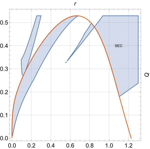
We note that the effective energy conditions of spacetime are badly damaged, especially the DEC. In addition, the NEC, the WEC, and the SEC are disrupted outside the horizon when $Q$ becomes small. To figure out which ingredient of matter is responsible for such damage, we draw the energy conditions associated with the scalar and monopole fields in Figs. 9 and 10, respectively.

It can be seen that the DEC of scalar and monopole fields is destroyed outside the horizon, whereas the NEC, WEC, and SEC are damaged outside the horizon by the monopole field when the charge is small. In addition, Fig. 8(c) demonstrates that the SEC is broken near $r=0$ even in the singular state, and such a violation is caused by the scalar field, which can be deduced when we compare Fig. 9(c) with Fig. 10(c). As a result, it is not possible to give the reason for the existence of singularity just from the point of view of energy conditions. Perhaps we need to start with the complete theory of geodesic convergence and then analyze Raychaudhuri’s equation [42].

We write down the equation of a massless scalar field [77, 78, 79],

$$\frac{1}{\sqrt{-g}}\partial_{\mu}\left(\sqrt{-g}g^{\mu\nu}\partial_{\nu}\Phi\right)=0.$$

(56)

To separate the variables, we take the ansatz,

$$\Phi=\frac{\Psi(r)}{r}Y_{l}^{m}(\theta,\phi)\mathrm{e}^{-\mathrm{i}\omega t},$$

(57)

and then obtain the equation satisfied by the radial component,

$$\frac{\mathrm{d}^{2}\Psi}{\mathrm{d}r_{*}^{2}}+\omega^{2}\Psi=V_{\rm eff}(r)\Psi,$$

(58)

where $\displaystyle r_{*}\coloneqq\int\mathrm{d}r/f(r)$ denotes the tortoise coordinate and the effective potential reads

$$V_{\rm eff}(r)=f(r)\left[\frac{l(l+1)}{r^{2}}+\frac{f^{\prime}(r)}{r}\right].$$

(59)

Substituting the shape function Eq. (22) into the above equation, we plot the effective potential for three $Q$ values in Fig. 11, where Fig. 11(a) is for $V(r)$ and Fig. 11(b) for $V(r_{*})$.

The shape of the effective potential implies that we are dealing with a scattering problem. The so-called quasinormal modes are defined as the solution of Eq. (58) satisfying the particular boundary conditions,

$$\Psi\sim\mathrm{e}^{\pm\mathrm{i}\omega r_{*}},\qquad r_{*}\to\pm\infty.$$

(60)

To compute the QNFs, we use the 13th-order WKB approach improved by the Padé approximation [70, 71].

For a specific value of $l=6$, we compute the QNFs with different values of $Q$. The relation is shown in Fig. 12, where we find the curves that fit the data best via the polynomials of $Q$.

The linear relation of the real part of the QNFs with charge is obvious in Fig. 12(a), where the fit line is of the form,

$$y=c_{1}x+c_{0},$$

(61)

with $c_{1}\approx 0.8989$ and $c_{0}\approx 2.1675$. However, the imaginary part shows the nonlinear relation with respect to the charge,

$$y=c_{4}x^{4}+c_{3}x^{3}+c_{2}x^{2}+c_{1}x+c_{0},$$

(62)

where the fit coefficients take the values as follows:

$$c_{0}\approx 0.1798,\quad c_{1}\approx 0.0594,\quad c_{2}\approx-0.2010,\quad c_{3}\approx 0.6202,\quad c_{4}\approx-1.0660.$$

(63)

Fig. 13 depicts the relationship between $\Re(\omega)$ and $-\Im(\omega)$ with more values of charge $Q\in[0,Q_{\rm ext}]$ and multipole number $l\in[1,10]$, where the frequencies with the same multipole number $l$ are joined into a curve. Meanwhile, all curves have a similar shape: One global minimum is located at $Q_{\rm ext}$ and one global maximum at a critical value $Q_{\rm C}$.

We calculate these critical values $Q_{\rm C}$ for a varying multipole number $l\in[1,10]$ and their corresponding QNFs, see Tab. 1.

The data circled by the red boxes in Tab. 1 show a possible phenomenon that $Q_{\rm C}$ and $-\Im(\omega)$ converge to constants in the eikonal limit ($l\gg 1$).

To provide an analytic result for the QNFs, we apply the light ring/QNMs correspondence [72], according to which the QNFs can be cast in the following form,

$$\omega=\Omega_{c}\,l-\mathrm{i}\left(n+\frac{1}{2}\right)|\lambda_{c}|,$$

(64)

where $\Omega_{c}$ denotes the angular velocity of a test scalar particle moving along an unstable null geodesic and $\lambda_{c}$ is the Lyapunov exponent. The applicability of this correspondence is limited, as evidenced by the case of the Einstein-Lovelock theory [80]. Furthermore, if the magnetic field’s influence on photon spheres is disregarded in our model, the correspondence is valid. However, if the magnetic field’s influence on photon spheres is considered, the correspondence is invalid, as in the cases discussed in Refs. [39, 81]. Note that the subscript $c$ means that the angular velocity and Lyapunov exponent are calculated at the radius of a circular null geodesic, $r_{c}$, determined by

$$2f_{c}=r_{c}f^{\prime}_{c},$$

(65)

where $f_{c}:=f(r_{c})$ and a prime means the derivative with respect to $r$. Thus we have [73]

$$\Omega_{c}^{2}=\frac{f_{c}}{r_{c}^{2}},\qquad\lambda_{c}^{2}=\frac{f_{c}}{2r_{c}^{2}}\left(2f_{c}-r_{c}^{2}f^{\prime\prime}_{c}\right).$$

(66)

For the shape function Eq. (22), we obtain the equation of a photon sphere,

$$Q^{3}r_{c}\left(Q-Q_{\rm{ext}}\right)^{2}+4r_{c}^{4}\left(Q-Q_{\rm{ext}}\right)^{2}-2\left(r_{c}^{3}+Q^{3}\right)^{2}+3r_{c}^{5}=0,$$

(67)

the angular velocity,

	$$\Omega_{c}^{2}=\frac{-r_{c}\left(Q-Q_{\rm ext}\right){}^{2}+r_{c}^{3}-r_{c}^{2}+Q^{3}}{r_{c}^{2}\left(r_{c}^{3}+Q^{3}\right)},$$		(68a)
and the Lyapunov exponent,
	$$\begin{split}\lambda_{c}^{2}r_{c}^{2}\left(r_{c}^{3}+Q^{3}\right)^{4}=&\left[-r_{c}\left(Q-Q_{\rm{ext}}\right){}^{2}+r_{c}^{3}-r_{c}^{2}+Q^{3}\right]\\ &\times\Big[-Q^{6}r_{c}\left(Q-Q_{\rm{ext}}\right)^{2}-8Q^{3}r_{c}^{4}\left(Q-Q_{\rm{ext}}\right)^{2}\\ &\;\;\;\;\;\;+2r_{c}^{7}\left(Q-Q_{\rm{ext}}\right)^{2}+3Q^{6}r_{c}^{3}+3Q^{3}r_{c}^{6}-9Q^{3}r_{c}^{5}+r_{c}^{9}+Q^{9}\Big],\end{split}$$		(68b)

respectively. The dependencies of $\Omega_{c}$ and $\lambda_{c}$ on $Q$ are shown in Fig. 14.

References

- [1] I. Dymnikova, “Vacuum nonsingular black hole,” Gen. Rel. Grav. 24 (1992) 235–242.
- [2] A. Bogojevic and D. Stojkovic, “A Nonsingular black hole,” Phys. Rev. D 61 (2000) 084011, arXiv:gr-qc/9804070.
- [3] S. A. Hayward, “Formation and evaporation of regular black holes,” Phys. Rev. Lett. 96 (2006) 031103, arXiv:gr-qc/0506126.
- [4] K. A. Bronnikov, V. N. Melnikov, and H. Dehnen, “Regular black holes and black universes,” Gen. Rel. Grav. 39 (2007) 973–987, arXiv:gr-qc/0611022.
- [5] S. Ansoldi, “Spherical black holes with regular center: A Review of existing models including a recent realization with Gaussian sources,” in Conference on Black Holes and Naked Singularities. 2, 2008. arXiv:0802.0330 [gr-qc].
- [6] P. Nicolini, “Noncommutative Black Holes, The Final Appeal To Quantum Gravity: A Review,” Int. J. Mod. Phys. A 24 (2009) 1229–1308, arXiv:0807.1939 [hep-th].
- [7] V. P. Frolov, “Notes on nonsingular models of black holes,” Phys. Rev. D 94 no. 10, (2016) 104056, arXiv:1609.01758 [gr-qc].
- [8] W. Berej, J. Matyjasek, D. Tryniecki, and M. Woronowicz, “Regular black holes in quadratic gravity,” Gen. Rel. Grav. 38 (2006) 885–906, arXiv:hep-th/0606185.
- [9] K. A. Bronnikov and J. C. Fabris, “Regular phantom black holes,” Phys. Rev. Lett. 96 (2006) 251101, arXiv:gr-qc/0511109.
- [10] E. Ayon-Beato and A. Garcia, “Regular black hole in general relativity coupled to nonlinear electrodynamics,” Phys. Rev. Lett. 80 (1998) 5056–5059, arXiv:gr-qc/9911046.
- [11] K. A. Bronnikov, “Regular magnetic black holes and monopoles from nonlinear electrodynamics,” Phys. Rev. D 63 (2001) 044005, arXiv:gr-qc/0006014.
- [12] E. Ayon-Beato and A. Garcia, “Four parametric regular black hole solution,” Gen. Rel. Grav. 37 (2005) 635, arXiv:hep-th/0403229.
- [13] L. Balart and E. C. Vagenas, “Regular black holes with a nonlinear electrodynamics source,” Phys. Rev. D 90 no. 12, (2014) 124045, arXiv:1408.0306 [gr-qc].
- [14] Z.-Y. Fan and X. Wang, “Construction of Regular Black Holes in General Relativity,” Phys. Rev. D 94 no. 12, (2016) 124027, arXiv:1610.02636 [gr-qc].
- [15] B. Toshmatov, Z. Stuchlík, and B. Ahmedov, “Comment on “Construction of regular black holes in general relativity”,” Phys. Rev. D 98 no. 2, (2018) 028501, arXiv:1807.09502 [gr-qc].
- [16] J. Vrba, A. Abdujabbarov, A. Tursunov, B. Ahmedov, and Z. Stuchlík, “Particle motion around generic black holes coupled to non-linear electrodynamics,” Eur. Phys. J. C 79 no. 9, (2019) 778, arXiv:1909.12026 [gr-qc].
- [17] J. Vrba, A. Abdujabbarov, M. Kološ, B. Ahmedov, Z. Stuchlík, and J. Rayimbaev, “Charged and magnetized particles motion in the field of generic singular black holes governed by general relativity coupled to nonlinear electrodynamics,” Phys. Rev. D 101 no. 12, (2020) 124039.
- [18] K. A. Bronnikov and R. K. Walia, “Field sources for Simpson-Visser spacetimes,” Phys. Rev. D 105 no. 4, (2022) 044039, arXiv:2112.13198 [gr-qc].
- [19] E. Greenwood and D. Stojkovic, “Quantum gravitational collapse: Non-singularity and non-locality,” JHEP 06 (2008) 042, arXiv:0802.4087 [gr-qc].
- [20] J. E. Wang, E. Greenwood, and D. Stojkovic, “Schrodinger formalism, black hole horizons and singularity behavior,” Phys. Rev. D 80 (2009) 124027, arXiv:0906.3250 [hep-th].
- [21] L. Modesto, “Super-renormalizable Quantum Gravity,” Phys. Rev. D 86 (2012) 044005, arXiv:1107.2403 [hep-th].
- [22] A. Saini and D. Stojkovic, “Nonlocal (but also nonsingular) physics at the last stages of gravitational collapse,” Phys. Rev. D 89 no. 4, (2014) 044003, arXiv:1401.6182 [gr-qc].
- [23] A. Ashtekar, J. Olmedo, and P. Singh, “Regular black holes from Loop Quantum Gravity,” arXiv:2301.01309 [gr-qc].
- [24] A. Bonanno and M. Reuter, “Renormalization group improved black hole space-times,” Phys. Rev. D 62 (2000) 043008, arXiv:hep-th/0002196.
- [25] M. A. Markov, “Limiting density of matter as a universal law of nature,” JETP Letters 36 (1982) 266. http://jetpletters.ru/ps/1334/article_20160.pdf.
- [26] R. Carballo-Rubio, F. Di Filippo, S. Liberati, and M. Visser, “Geodesically complete black holes,” Phys. Rev. D 101 (2020) 084047, arXiv:1911.11200 [gr-qc].
- [27] R. Carballo-Rubio, F. Di Filippo, S. Liberati, and M. Visser, “Geodesically complete black holes in Lorentz-violating gravity,” JHEP 02 (2022) 122, arXiv:2111.03113 [gr-qc].
- [28] R. P. Geroch, “What is a singularity in general relativity?,” Annals Phys. 48 (1968) 526–540.
- [29] G. J. Olmo, D. Rubiera-Garcia, and A. Sanchez-Puente, “Geodesic completeness in a wormhole spacetime with horizons,” Phys. Rev. D 92 no. 4, (2015) 044047, arXiv:1508.03272 [hep-th].
- [30] R. M. Wald, General Relativity. Chicago Univ. Pr., Chicago, USA, 1984.
- [31] S. M. Carroll, Spacetime and Geometry. Cambridge University Press, 7, 2019.
- [32] T. Zhou and L. Modesto, “Geodesic incompleteness of some popular regular black holes,” Phys. Rev. D 107 no. 4, (2023) 044016, arXiv:2208.02557 [gr-qc].
- [33] K. A. Bronnikov, R. A. Konoplya, and A. Zhidenko, “Instabilities of wormholes and regular black holes supported by a phantom scalar field,” Phys. Rev. D 86 (2012) 024028, arXiv:1205.2224 [gr-qc].
- [34] S. Fernando and J. Correa, “Quasinormal Modes of Bardeen Black Hole: Scalar Perturbations,” Phys. Rev. D 86 (2012) 064039, arXiv:1208.5442 [gr-qc].
- [35] A. Flachi and J. P. S. Lemos, “Quasinormal modes of regular black holes,” Phys. Rev. D 87 no. 2, (2013) 024034, arXiv:1211.6212 [gr-qc].
- [36] B. Toshmatov, A. Abdujabbarov, Z. Stuchlík, and B. Ahmedov, “Quasinormal modes of test fields around regular black holes,” Phys. Rev. D 91 no. 8, (2015) 083008, arXiv:1503.05737 [gr-qc].
- [37] A. Abdujabbarov, M. Amir, B. Ahmedov, and S. G. Ghosh, “Shadow of rotating regular black holes,” Phys. Rev. D 93 no. 10, (2016) 104004, arXiv:1604.03809 [gr-qc].
- [38] R. Kumar, S. G. Ghosh, and A. Wang, “Shadow cast and deflection of light by charged rotating regular black holes,” Phys. Rev. D 100 no. 12, (2019) 124024, arXiv:1912.05154 [gr-qc].
- [39] Z. Stuchlík and J. Schee, “Shadow of the regular Bardeen black holes and comparison of the motion of photons and neutrinos,” Eur. Phys. J. C 79 no. 1, (2019) 44.
- [40] C. Liu, T. Zhu, Q. Wu, K. Jusufi, M. Jamil, M. Azreg-Aïnou, and A. Wang, “Shadow and quasinormal modes of a rotating loop quantum black hole,” Phys. Rev. D 101 no. 8, (2020) 084001, arXiv:2003.00477 [gr-qc]. [Erratum: Phys.Rev.D 103, 089902 (2021)].
- [41] Y. S. Myung, Y.-W. Kim, and Y.-J. Park, “Thermodynamics of regular black hole,” Gen. Rel. Grav. 41 (2009) 1051–1067, arXiv:0708.3145 [gr-qc].
- [42] C. Lan and Y.-G. Miao, “Gliner vacuum, self-consistent theory of Ruppeiner geometry for regular black holes,” Eur. Phys. J. C 82 no. 12, (2022) 1152, arXiv:2103.14413 [gr-qc].
- [43] R. A. Konoplya, A. F. Zinhailo, J. Kunz, Z. Stuchlik, and A. Zhidenko, “Quasinormal ringing of regular black holes in asymptotically safe gravity: the importance of overtones,” JCAP 10 (2022) 091, arXiv:2206.14714 [gr-qc].
- [44] S. Vagnozzi et al., “Horizon-scale tests of gravity theories and fundamental physics from the Event Horizon Telescope image of Sagittarius A∗,” arXiv:2205.07787 [gr-qc].
- [45] R. A. Konoplya, Z. Stuchlik, A. Zhidenko, and A. F. Zinhailo, “Quasinormal modes of renormalization group improved Dymnikova regular black holes,” arXiv:2303.01987 [gr-qc].
- [46] V. P. Frolov, M. A. Markov, and V. F. Mukhanov, “Black Holes as Possible Sources of Closed and Semiclosed Worlds,” Phys. Rev. D 41 (1990) 383.
- [47] V. P. Frolov and A. Zelnikov, “Spherically symmetric black holes in the limiting curvature theory of gravity,” Phys. Rev. D 105 no. 2, (2022) 024041, arXiv:2111.12846 [gr-qc].
- [48] S. W. Hawking and G. F. R. Ellis, The Large Scale Structure of Space-Time. Cambridge Monographs on Mathematical Physics. Cambridge University Press, 2, 2011.
- [49] E. Zakhary and C. B. G. Mcintosh, “A complete set of riemann invariants,” General Relativity and Gravitation 29 (1997) 539–581.
- [50] S. Weinberg, Gravitation and Cosmology: Principles and Applications of the General Theory of Relativity. John Wiley and Sons, New York, 1972.
- [51] V. Pravda, A. Pravdova, A. Coley, and R. Milson, “All space-times with vanishing curvature invariants,” Class. Quant. Grav. 19 (2002) 6213–6236, arXiv:gr-qc/0209024.
- [52] G. V. Kraniotis, “Curvature Invariants for accelerating Kerr-Newman black holes in (anti-)de Sitter spacetime,” Class. Quant. Grav. 39 (2022) 145002, arXiv:2112.01235 [gr-qc].
- [53] J. Overduin, M. Coplan, K. Wilcomb, and R. C. Henry, “Curvature invariants for charged and rotating black holes,” Universe 6 no. 2, (2020) 22.
- [54] R. Torres and F. Fayos, “On regular rotating black holes,” Gen. Rel. Grav. 49 no. 1, (2017) 2, arXiv:1611.03654 [gr-qc].
- [55] S. Chandrasekhar, The mathematical theory of black holes. Oxford university press, 1985.
- [56] K. Martel and E. Poisson, “Regular coordinate systems for Schwarzschild and other spherical spacetimes,” Am. J. Phys. 69 no. 4, (Apr., 2001) 476–480, arXiv:gr-qc/0001069 [gr-qc].
- [57] G.-R. Liang and W.-B. Liu, “Geodesics in generalized painlevé-gullstrand coordinates and tunneling process from a schwarzschild black hole,” Int. J. Theor. Phys. 54 (2015) 3397–3401.
- [58] A. Simpson and M. Visser, “Black-bounce to traversable wormhole,” JCAP 02 (2019) 042, arXiv:1812.07114 [gr-qc].
- [59] M. S. Churilova and Z. Stuchlik, “Ringing of the regular black-hole/wormhole transition,” Class. Quant. Grav. 37 no. 7, (2020) 075014, arXiv:1911.11823 [gr-qc].
- [60] T. P. Sotiriou and V. Faraoni, “f(R) Theories Of Gravity,” Rev. Mod. Phys. 82 (2010) 451–497, arXiv:0805.1726 [gr-qc].
- [61] I. V. Dolgachev, Classical Algebraic Geometry: A Modern View. Cambridge University Press, 2012.
- [62] H. Stephani, D. Kramer, M. A. H. MacCallum, C. Hoenselaers, and E. Herlt, Exact solutions of Einstein’s field equations. Cambridge Monographs on Mathematical Physics. Cambridge Univ. Press, Cambridge, 2003.
- [63] A. A. Starobinsky, “A New Type of Isotropic Cosmological Models Without Singularity,” Phys. Lett. B 91 (1980) 99–102.
- [64] K. A. Bronnikov, “Comment on “Construction of regular black holes in general relativity”,” Phys. Rev. D 96 no. 12, (2017) 128501, arXiv:1712.04342 [gr-qc].
- [65] O. B. Zaslavskii, “Regular black holes and energy conditions,” Phys. Lett. B 688 (2010) 278–280, arXiv:1004.2362 [gr-qc].
- [66] H. Maeda, “Quest for realistic non-singular black-hole geometries: regular-center type,” JHEP 11 (2022) 108, arXiv:2107.04791 [gr-qc].
- [67] B. Toshmatov, C. Bambi, B. Ahmedov, A. Abdujabbarov, and Z. Stuchlík, “Energy conditions of non-singular black hole spacetimes in conformal gravity,” Eur. Phys. J. C 77 no. 8, (2017) 542, arXiv:1702.06855 [gr-qc].
- [68] C. Lan, Y.-G. Miao, and Y.-X. Zang, “Acoustic regular black hole in fluid and its similarity and diversity to a conformally related black hole,” Eur. Phys. J. C 82 no. 3, (2022) 231, arXiv:2109.13556 [gr-qc].
- [69] C. Lan, Y.-G. Miao, and Y.-X. Zang, “Regular black holes with improved energy conditions and their analogues in fluids*,” Chin. Phys. C 47 no. 5, (2023) 052001, arXiv:2206.08694 [gr-qc].
- [70] J. Matyjasek and M. Opala, “Quasinormal modes of black holes. The improved semianalytic approach,” Phys. Rev. D 96 no. 2, (2017) 024011, arXiv:1704.00361 [gr-qc].
- [71] R. A. Konoplya, A. Zhidenko, and A. F. Zinhailo, “Higher order WKB formula for quasinormal modes and grey-body factors: recipes for quick and accurate calculations,” Class. Quant. Grav. 36 (2019) 155002, arXiv:1904.10333 [gr-qc].
- [72] V. Cardoso, A. S. Miranda, E. Berti, H. Witek, and V. T. Zanchin, “Geodesic stability, Lyapunov exponents and quasinormal modes,” Phys. Rev. D 79 no. 6, (2009) 064016, arXiv:0812.1806 [hep-th].
- [73] S.-W. Wei and Y.-X. Liu, “Null Geodesics, Quasinormal Modes, and Thermodynamic Phase Transition for Charged Black Holes in Asymptotically Flat and dS Spacetimes,” Chin. Phys. C 44 no. 11, (2020) 115103, arXiv:1909.11911 [gr-qc].
- [74] L. Motl and A. Neitzke, “Asymptotic black hole quasinormal frequencies,” Adv. Theor. Math. Phys. 7 no. 2, (Jan., 2003) 307–330, arXiv:hep-th/0301173 [hep-th].
- [75] J. Natario and R. Schiappa, “On the classification of asymptotic quasinormal frequencies for d-dimensional black holes and quantum gravity,” Adv. Theor. Math. Phys. 8 no. 6, (2004) 1001–1131, arXiv:hep-th/0411267.
- [76] C. Lan and Y.-F. Wang, “Singularities of regular black holes and the monodromy method for asymptotic quasinormal modes,” Chin. Phys. C 47 no. 2, (2023) 025103, arXiv:2205.05935 [gr-qc].
- [77] K. D. Kokkotas and B. G. Schmidt, “Quasinormal modes of stars and black holes,” Living Rev. Rel. 2 (1999) 2, arXiv:gr-qc/9909058.
- [78] E. Berti, V. Cardoso, and A. O. Starinets, “Quasinormal modes of black holes and black branes,” Class. Quant. Grav. 26 (2009) 163001, arXiv:0905.2975 [gr-qc].
- [79] R. A. Konoplya and A. Zhidenko, “Quasinormal modes of black holes: From astrophysics to string theory,” Rev. Mod. Phys. 83 (2011) 793–836, arXiv:1102.4014 [gr-qc].
- [80] R. A. Konoplya and Z. Stuchlík, “Are eikonal quasinormal modes linked to the unstable circular null geodesics?,” Phys. Lett. B 771 (2017) 597–602, arXiv:1705.05928 [gr-qc].
- [81] B. Toshmatov, Z. Stuchlík, B. Ahmedov, and D. Malafarina, “Relaxations of perturbations of spacetimes in general relativity coupled to nonlinear electrodynamics,” Phys. Rev. D 99 no. 6, (2019) 064043, arXiv:1903.03778 [gr-qc].
- [82] I. R. Shafarevich, Basic Algebraic Geometry 1. Springer Berlin Heidelberg, 2013. https://doi.org/10.1007%2F978-3-642-37956-7.
- [83] R. M. Wald, “Black hole entropy is the Noether charge,” Phys. Rev. D 48 no. 8, (1993) R3427–R3431, arXiv:gr-qc/9307038.
- [84] G. W. Gibbons and S. W. Hawking, “Action Integrals and Partition Functions in Quantum Gravity,” Phys. Rev. D 15 (1977) 2752–2756.
- [85] T. Jacobson, G. Kang, and R. C. Myers, “On black hole entropy,” Phys. Rev. D 49 (1994) 6587–6598, arXiv:gr-qc/9312023.
- [86] P. C. W. Davies, “Thermodynamics of Black Holes,” Proc. Roy. Soc. Lond. A 353 (1977) 499–521.
- [87] C. Lan, Y.-G. Miao, and H. Yang, “Quasinormal modes and phase transitions of regular black holes,” Nucl. Phys. B 971 (2021) 115539, arXiv:2008.04609 [gr-qc].
- [88] S. A. H. Mansoori and B. Mirza, “Correspondence of phase transition points and singularities of thermodynamic geometry of black holes,” Eur. Phys. J. C 74 no. 99, (2014) 2681, arXiv:1308.1543 [gr-qc].
- [89] H. Quevedo and M. N. Quevedo, “Unified representation of homogeneous and quasi-homogenous systems in geometrothermodynamics,” Phys. Lett. B 838 (2023) 137678.
- [90] S. H. Hendi, S. Panahiyan, B. Eslam Panah, and M. Momennia, “A new approach toward geometrical concept of black hole thermodynamics,” Eur. Phys. J. C 75 no. 10, (2015) 507, arXiv:1506.08092 [gr-qc].
- [91] S.-W. Wei, Y.-X. Liu, and R. B. Mann, “Repulsive Interactions and Universal Properties of Charged Anti–de Sitter Black Hole Microstructures,” Phys. Rev. Lett. 123 no. 7, (2019) 071103, arXiv:1906.10840 [gr-qc].
- [92] S.-W. Wei, Y.-X. Liu, and R. B. Mann, “Ruppeiner Geometry, Phase Transitions, and the Microstructure of Charged AdS Black Holes,” Phys. Rev. D 100 no. 12, (2019) 124033, arXiv:1909.03887 [gr-qc].
- [93] G. Ruppeiner, “Riemannian geometry in thermodynamic fluctuation theory,” Rev. Mod. Phys. 67 (1995) 605–659. [Erratum: Rev.Mod.Phys. 68, 313–313 (1996)].
- [94] H. Quevedo, “Geometrothermodynamics,” J. Math. Phys. 48 (2007) 013506, arXiv:physics/0604164.
- [95] H. Quevedo, “Geometrothermodynamics of black holes,” Gen. Rel. Grav. 40 (2008) 971–984, arXiv:0704.3102 [gr-qc].
- [96] R. Tharanath, J. Suresh, and V. C. Kuriakose, “Phase transitions and Geometrothermodynamics of Regular black holes,” Gen. Rel. Grav. 47 no. 4, (2015) 46, arXiv:1406.3916 [gr-qc].
- [97] R. Ghosh, M. Rahman, and A. K. Mishra, “Regularized stable Kerr black hole: cosmic censorships, shadow and quasi-normal modes,” Eur. Phys. J. C 83 no. 1, (2023) 91, arXiv:2209.12291 [gr-qc].
- [98] H. Yang and Y.-G. Miao, “Superradiance of massive scalar particles around rotating regular black holes*,” Chin. Phys. C 47 no. 7, (2023) 075101, arXiv:2211.15130 [gr-qc].
- [99] M. Azreg-Aïnou, “Generating rotating regular black hole solutions without complexification,” Phys. Rev. D 90 no. 6, (2014) 064041, arXiv:1405.2569 [gr-qc].
- [100] M. Azreg-Aïnou, “From static to rotating to conformal static solutions: Rotating imperfect fluid wormholes with(out) electric or magnetic field,” Eur. Phys. J. C 74 no. 5, (2014) 2865, arXiv:1401.4292 [gr-qc].