Tunability of Andreev levels in a spin-active Ising Superconductor/Half Metal Josephson junction
Abstract
We study the Andreev levels, supercurrent and tunnelling conductance in a clean Ising superconductor (ISC)/half metal (HM)/Ising superconductor (ISC) Josephson junction with spin-active interfaces using Bogoliubov-de Gennes equations. We theoretically demonstrate the effect of spin mixing, spin flipping processes and spin-orbit coupling (SOC) of the ISC on Andreev Bound States (ABS) spectra, current phase relation (CPR) and tunnelling conductance in transparent and opaque barrier limit. We witness an additional splitting of the Andreev levels due to SOC of the ISC and transition for different barrier magnetic moments. Also, different - junctions can be achieved by tuning the strength of the barrier magnetic moment and spin mismatch angle. Moreover, a possible transition can also be achieved for SOC stronger than the chemical potential of the ISC using suitable control parameters. The interplay of spin mixing and spin flipping processes with SOC can also host Majorana modes in the proposed system. The tunnelling conductance is found to be dependent on the spin mismatch angle. Also, a finite sub-gap conductance is observed, which indicates different probabilities of Andreev reflected electrons and holes in the presence of SOC. Furthermore, anomalous Andreev levels are observed for different HM length scales signifying its role in the tunability of the - phase Josephson junction.
pacs
74.45.+c, 85.75.-d, 74.90.+n, 75.76.+jI Introduction
The exhibition of superconductivity and magnetism in the same domain leads to several engrossing phenomena saxena; aoki; pfleiderer; ginsburg; zutic; buzdin; acharjee1; hirai; andreev. In general spin-singlet superconductivity has a detrimental effect with a strong magnetic field andreev; ginsburg; hirai. Nevertheless, the discovery of long-range superconductivity in two-dimensional monolayer transition-metal dichalcogenides (TMD) like MoS2, NbSe2, TaS2, WSe2 etc., open up a new dimension in superconducting spintronics barrera; idzuchi; jalouli; taguchi; scharf; tang; lu; saito; xi; dvir; costanzo; sohn; li; hamil; ai. Monolayer TMD - superconductors lack in-plane mirror symmetry, resulting in strong antisymmetric spin-orbit coupling (SOC). So, they admit both spin-singlet and spin-triplet components of the superconducting wave function. Moreover, due to the lack of inversion symmetry and strong SOC, the electrons near the and -valleys witness a strong Zeeman field more enormous than the Pauli limit, leading to long-range superconductivity lu; saito; xi; dvir; costanzo; sohn; li; hamil; ai; zhu2; xiao2; kormanyos; cappelluti. It is to be noted that the Andreev reflection process is significantly suppressed in conventional HMS heterostructure andreev; ginsburg; hirai. However, half metal (HM)Ising Superconductor (ISC) junctions can offer spin-triplet Andreev reflection due to the formation of equal spin Cooper pairs when the alignment of the HM magnetic moments is parallel to the plane of HMISC junction zhou; lv; cheng. Furthermore, spin-triplet pairing will lead to nontrivial topological superconductivity supporting Majorana edge states zhou.
Thus, the magnetic heterostructure and Josephson junctions (JJ) have widely been explored theoretically and experimentally huy; flouquet; nandi; banerjee; acharjee2; acharjee3. Efforts have been made to realize the coexistence of and states in the junction region and to fabricate a tunable - phase JJ, which can be used as a quantum phase battery strambini. Moreover, different phases can be utilized to fabricate quantum qubit devices and cryogenic memories for next-generation quantum computing based on the currently available semiconductor technology ioffe; ioffe2; hilgenkamp; madden. A - phase JJ can offer a constant phase bias in open circuit configuration resulting in the current phase relation (CPR), buzdin2. However, the closed superconducting loop will induce an anomalous Josephson current, . It is to be noted that or - phase JJ can be easily engineered if the time-reversal symmetry () is broken strambini. However, in the absence of both time reversal () and inversion symmetries (), a finite phase shift in the CPR will be induced. Since, lateral hybrid arrangements break the inversion symmetry, they possess strong SOC. Thus lateral junctions with ISC or topological insulators are the promising candidate to engineer Josephson junction szombati; assouline; mayer.
The JJs with spin-active interfaces or magnetic impurities can offer spin-sensitive Andreev reflection, supporting unconventional long-range spin-triplet correlations keizer1; khaire; linder1; eschrig; acharjee4. The long-range spin-triplet superconducting correlation in such JJs is mainly due to the combination of spin mixing and spin-flip scattering processes eschrig2; galaktionov; eschrig; acharjee4; millis; hubler; kalenkov. Experimentally, magnetic JJ with spin-active interfaces can be possibly realized by placing a thin magnetic layer at the interface. The barrier spin moments in such JJ are still uncontrollable as it is its inherent property. However, a well engineered spin-active interface can host and control the barrier spin moments through non-equilibrium spin injection process at the interface ouassou; zwierzycki; jeon; bobkova. Supercurrent control and anomalous conductivities have been explored in superconductor-ferromagnetic geometries jeon. Due to a spin-active barrier moment, the transmission profile of up-spin and down-spin electrons at the interface are significantly different and can be controlled through the spin-mixing angle. Moreover, the impact of spin-flip scattering on Josephson supercurrent and CPR has also been studied in a spin active SHMS JJ galaktionov; kalenkov; millis. Very recently, the switch effect has been explored in ISCFM JJs cheng. The transport properties of ISCHM hybrids and JJs have also been explored theoretically dai. However, from the best of our knowledge, the Ising Superconductor/half metallic heterostructure with spin active interfaces is yet to be explored. So, in this work, we consider an ISCHMISC JJ with spin-active interfaces. The present work is focusses on understanding the superconducting spin-triplet correlations and the interplay between spin-dependent barrier moment, SOC of the ISC concerning (i) Andreev levels, (ii) Majorana modes and (iii) Josephson supercurrent.
The paper’s organization is as follows: Section II defines the Bogoliubov de-Gennes Hamiltonian and discusses a theoretical formulation of the proposed geometry. The Andreev Bound States (ABS) and the supercurrent of the proposed system are studied in Section III. In Section IV, the results of our work are discussed. A brief note on realization of the proposed experimental setup and concluding remarks of our work is presented in Section V.
II Formulation
We consider a half-metallic (HM) ferromagnet sandwiched between two Ising Superconductors (ISC) as shown in Fig. 1(a). The ISCHMISC Josephson junction is supposed to satisfy the condition , where L is the length of the HM, and is the superconducting coherence length. The magnetization of the bulk HM is directed along the z direction, and the ISCHM interface is spin active. So, the barrier magnetic moments constitute a spin-dependent potential defined as , where, is the intrinsic spin independent barrier potential. The parameter characterize the effective ratio of barrier magnetic and non-magnetic moments, and the angles and represents the polar and the azimuthal angular components of the magnetic barrier moment made with the bulk moment of the HM.
Using Nambu basis, the Bogoliubov de-Gennes (BdG) equation of the system can be written as , where BdG Hamiltonian can be defined as acharjee4; cheng
| (1) |
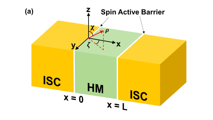

where is the single particle Hamiltonian which in the presence of the two valleys ( and ) of ISC can be written as tang
| (2) |
where is the wave vectors of the electron corresponding to the valley , are the chemical potentials of the respective layers and is the valley index for . The schematic energy band of the ISC is displayed in Fig. 1(b). The up and down spin subbands split into constituents due to the SOC of the ISC. It is to be noted that the spin-up band has higher energy than spin-down bands at valley, while an opposite characteristic is observed for valley. The parameter characterize the strength of spin-orbit coupling of ISC while is the barrier potential at ISCHM interfaces and can be defined as acharjee4; kalenkov
| (3) |
The term in Eq. (1) represents the exchange field of the system and can be defined as
| (4) |
where, the parameter, represent the magnetization of the bulk HM and = () are the Pauli’s spin matrices. Since the spin polarization of the bulk HM is completely along the z-direction, we can write .
The superconducting pair potential for the left and right ISC appearing in Eq. (1) can be defined as tang
| (5) |
where is the superconducting gap magnitude and correspond to the superconducting phase of the left (right) ISC. So, the phase difference of the left and right ISC can be written as . The wave function in the ISC regions can be obtained by considering and solving the BdG equation. Using plane wave assumption and diagonalizing the Hamiltonian from Eq.(1), the wave function in the left ISC can be defined as cheng
| (6) |
Similarly, the wave function of the right ISC can also be defined as
| (7) |
where we define, , , and . Here, () are the reflection coefficients for up (down) spin electrons while () are the reflection coefficients for the up (down) spin holes in left ISC region. () are the transmission coefficients for up(down) spin electrons while () are the transmission coefficients for the up(down) spin holes in right ISC region. gives the momenta of the electron (hole) in ISC. The momenta of the electron and the holes under the Andreev approximation can be defined as
| (8) |
where and , respectively, are the chemical potential and the strength of SOC in the ISC region. We also have considered for our analysis. The quasiparticle amplitudes and appearing in Eq.(8) are defined as
| (9) | |||
| (10) |
In a similar way, the wave function in the half-metallic region is linder1; acharjee4
| (11) |
where , , , are the scattering coefficients for electron and hole in the half-metallic region with corresponding to the wave function respectively. The quasi-particle momenta in this region are given by
| (12) |
where, is the chemical potential of the HM and (, , ) are the components of barrier magnetic moments. The schematic energy band of the HM is displayed in Fig. 1(c). The spin-up and spin-down subbands split into constituents due to the strong Zeeman field of the HM. The wave functions must satisfy the conditions:
| (13) | ||||
| (14) | ||||
| (15) | ||||
| (16) |
where, is a 44 identity matrix. The matrix gives the sum of spin-independent and spin-dependent barrier potential and has the following form linder1; acharjee4
| (17) |
where, represents the spin independent barrier strength while and are the terms corresponds to spin dependent barrier potential.

III Bound State energy and Supercurrent
The Andreev levels of the ISCHMISC Josephson junction can be obtained by using the boundary conditions Eqs. (13)-(16). This indeed gives rise to a system of equations given by , where is a 1616 matrix carrying all the information regarding the bound state energies and . The bound state energies and the Andreev levels are obtained by using the condition . where, represent the determinent of the matrix. An extensive form of is presented in Appendix (22). It is to be noted that the Andreev levels satisfy the equality cheng. So, in our analysis, only the results of Andreev levels are displayed.
An expression for the normalized Josephson supercurrent can be obtained by using the standard expression linder1; acharjee4
| (18) |
where, and corresponds to the energies of the Andreev levels with . Here, is the angle of incidence of the incoming electron. We set, with represents the critical temperature of the ISC and . Moreover, to restrict our analysis to the interface, we consider the azimuthal angle for all our analyses. The supercurrent generally has dependence for large values of . So, we consider both low () and high () values of the barrier width. In our analysis, the spin mixing processes are achieved by considering and while spin mixing and spin flipping processes are obtained for and .


IV Andreev Bound States
IV.1 Andreev levels for a spin active barrier in absence of Spin-orbit coupling
Before we present the result of a spin-active ISCHMISC JJ, we have presented the Andreev energy levels in the absence of SOC which indeed represents a spin-active triplet SHMS JJ. We have considered different and values to understand the role of spin mixing and spin flipping on ABS spectra. In the absence of SOC, the Andreev levels are expressed by
| (19) |
where, we define , , and as
The Andreev energy levels from Eq. (19), are displayed in Fig. (2) for different barrier width (), barrier magnetic moment () and mismatch angle (). The ABS spectra are found to be degenerate for , which follows the results of a spin inactive conventional SFS JJ. A splitting of the two degenerate energy bands into four respective constituents is observed for , which arises solely due to the spin-mixing process in a spin-active barrier. However, the identical ABS spectra for different values indicate no impact of spin-flipping processes on Andreev levels. A signature of non-trivial Josephson phases and are observed as minimum energy for state in transparent () and intermediate () barrier width. However, the system favours the phase for an opaque barrier. The (, ) states are mostly located near - phase. However, as increase to , the (, ) - phases depart from , indicating the increase in the splitting of the Andreev levels. Moreover, in this configuration, the system resides in the phase for considered values, as seen from Figs. 2(b) and 2(c). As increases to , the two sets of Andreev levels depart further away from each other and tend to favour and phases. Thus for a fully magnetic and transparent barrier, one can observe and junctions. However, for a fully opaque barrier, the signature of junction is perceived from Fig. 2(d). Thus the results indicate the possibility of tunability via spin active barrier moment even in the absence of SOC. It is to be noted that the impact of spin flipping is absent for . Nevertheless, a possible Majorana mode can exist in a near-transparent barrier configuration due to the barrier spin moments tang.
IV.2 Andreev levels for a spin active barrier in presence of Spin-orbit coupling
In presence of SOC, the wave vectors , and are not identical. This mismatch can cause additional splitting of the Andreev energy bands. It is to be noted that an analytic expression for Andreev levels for is too challenging to obtain as both and has non-vanishing distinct values in this condition. So, we have used numerical simulation to present our result for . However, a possible analytic expression for a system with can still be obtained as vanishes in this condition. The Andreev energy levels for can be expressed as
| (20) |
where, we defined


Figs. 3(a) - 3(h) display the impact of barrier magnetic moment () and mismatch angle () on ABS spectra for transparent and opaque barrier configuration considering . The characteristics of the Andreev levels are similar with seen from Figs. 2(a) for transparent barrier configuration. The ABS bands are found to be degenerate in this case for as seen from Fig. 3(a). However, a splitting in ABS spectra is observed in Fig. 3(e) for opaque barrier configuration, which arises due to the inherent SOC of the ISC. With the rise in to , the degenerate Andreev bands split into eight constituents due to the combined effect of SOC and spin active barrier moment. It is to be noted that the and phases individually split into two different -states corresponding to the minima of the ABS spectra as indicated by Fig. 3(b). It is a consequence of different spin-flipping probabilities of the spin-up and spin-down electrons, which are unlocked due to SOC. So, it is possible to tune different states by considering suitable mismatch angles between the barrier and bulk moments. However, Andreev levels remain degenerate for , indicating equal spin flipping probability of up and down spin electrons. The Andreev bands split further with the increase in to . It is to be noted that there exists a possible phase shift for , indicating a possible junction. But a - phase JJ is observed for . Moreover, for a fully magnetic barrier, i.e., , the system prefers junction for all mismatch angles in both transparent and opaque barrier configurations, as seen from Figs. 3(d) and 3(h) respectively. Though splitting of the ABS bands is also observed with the increase in for , but a notable difference in ABS spectra is noticed for . In this case, the system prefers the phase for all choices of , as seen from Fig. 3(f). The splitting is further increased for ; in this condition, the system resides in state as seen from Fig. 3(g). Furthermore, the existence of -modes and the combined effect of barrier magnetic moment, mismatch angle and the SOC of the ISC can support Majorana mode acharjee4. So, it can be concluded that the tunability of junction can be achieved via SOC of ISC, magnetic barrier moment and spin mismatch angle.

IV.3 Current Phase Relation
The current phase relation (CPR) of ISCHMISC JJ are shown in Fig. 4 corresponding to the ABS spectra in Figs. 2 and 3. The Josephson supercurrents () are found to be similar to a conventional magnetic S/F/S junction in the absence of SOC linder1; acharjee4, as seen from Fig. 4(a). A signature of anomalous supercurrent is noted from Figs. 4(b)-4(d) for and . The system behaves like a -junction for and with . However, the characteristics of a -junction are still present for an opaque barrier (). The further increase in to restrict the system to reside only in -phase as indicated by Fig. 4(c). For a system with and , a phase shift of is noted. Though the system tends to behave like a junction, the signature of -state is still present for a system with barrier width and as seen from Fig. 4(d). So, it can be concluded that a -junction can be realized by choosing a suitable barrier width and barrier magnetic moment, even in the absence of SOC. Although the system is spin-active, the impact of is absent in the absence of SOC.
The plots in the middle and the bottom panel of Fig. 4 display the CPR for and , respectively. For a normal barrier with and , the supercurrent is found to be similar to , which is consistent with the ABS spectra in Fig. 3(a) and 3(e). However, the magnitude of decreases for due to the presence of component of the momenta. We observe the characteristics of a -junction for a system with , , and . As and phases of the ABS spectra differ for different mismatch angles [Fig. 3(b)], consequently different junctions are noted in the CPR. However, a - junction signature is observed for a system with . Moreover, the impact of mismatch angle is absent in this case, as seen from Fig. 4(f). For with , a transition from junction is noticed for mismatch angle . While for other mismatch angles, the system still prefers the - phases as indicated by Fig. 4(g). A possible junction is noticed for an opaque barrier (). The effect of the mismatch angle is suppressed, and a phase-shift of is noticed in for both and conditions indicated from Fig. 4(h). The effect of spin mismatch angle is enhanced for with . However, in the presence of spin magnetic moment with , the effect of spin-flipping is absent, resulting in a vanishing supercurrent. A signature of anomalous supercurrent is noticed in Figs. 4(j) - 4(l) for and , which is due to the presence of spin mixing and spin flipping processes for both transparent and opaque barrier conditions. Moreover, the presence of SOC and spin flipping enhances the tunability of -phase even in the opaque barrier. This indicates that ISCHM ISC-based JJ can be utilized to fabricate a tunable - junction more efficiently than the conventional JJs.
Fig. 5, display a comparative result of CPR between conventional spin-active SHMS JJ and a spin-active ISCHMISC JJ considering and . The impact of chemical potential () is shown in Figs. 5(a) and 5(b) considering while that of the length of the HM () is shown in Figs. 5(c) and 5(d) considering . For a system with , a possible - junction is observed while the system favours -phase for for and which is in accordance with the results of Ref[linder1. However, in case of with , the system tends to form - junction for . In case of opaque barrier (), a conventional spin-active JJ mostly reside in -phase while a spin-active ISCHMISC JJ favours -phase only for . In presence of SOC an anomalous -junction is observed for . Furthermore, apart from conventional - characteristics, additional spikes in CPR are observed for a spin-active ISCHMISC JJ in transparent barrier condition. It is due to the additional splitting of the bands solely by the inherent SOC leading to the mismatch of and vectors of ISC. It is noteworthy to mention that the system transits from to phase for both transparent and opaque conventional spin-active SHMS JJ as the is increased from to . However, a possible -junction is observed for all choices of in a spin-active ISCHMISC JJ.
IV.4 Andreev reflection and Tunnelling Conductance
The tunneling conductance in presence of SOC, spin mixing and spin flipping can be obtained by using the relation hashimoto; acharjee2; acharjee3; dai
| (21) |
where, and are the normal and Andreev reflection probabilities at the respective layers.


The tunnelling conductance of ISCHMISC JJ is shown in Fig. 6. The orientation () and phase () dependence of the conductance profile are displayed for and in Figs. 6(a) and 6(b) respectively considering , and . An asymmetric characteristic of the conductance spectra is observed for strong magnetic barriers in contrast to a low magnetic barrier due to the combined effect of SOC, spin mixing and spin flipping processes. It is to be noted that for a strong magnetic barrier, there exists a sudden dip in conductance profile in the region . The variation of conductance with energy () in terms of gap parameter () for spin mixing processes is shown in Fig. 7(c). At the same time, we consider a combined effect of spin mixing and spin flipping on conductance in Fig. 6 (d). We observe that the sharpness of the peak decreases with an increasing value of . Although the sub-gap conductance is zero for conventional SHMS JJ’s, a finite sub-gap conductance is observed in our proposed system. It is due to unequal probabilities of Andreev reflected electron and hole due to SOC. In the presence of spin-flipping processes with , the zero bias conductance peaks are found to be different for different mismatch angles. Moreover, the conductance peaks broaden and shift towards the low energy values with an increased mismatch angle, as shown in Fig. 6(d).

Fig. 7 displays the variation of gap energy as a function of and for spin mixing and spin-flipping processes. We observe a drastic change in the gap energy without spin flipping for weak and strong magnetic barriers. A signature of energy gap oscillation is observed with the change in . Though the system retains the characteristics of gap oscillation of a conventional JJ for but for , the oscillation maxima are found for , , and as seen from Figs. 7(a) and Fig. 7(b). In the presence of spin flipping, similar characteristics are seen for with , but a sharp splitting is seen at . It is to be noted for a strong magnetic barrier with , the oscillation maxima are observed at , which suggests no change in the superconducting phase. Moreover, energy gap maxima shrinks and arise in the vicinity of , , and as observed from Fig. 7(d).
The results of this work are also consistent with the results for the diffusive limit. It is primarily due to the following: (1) The states and thus the anomalous supercurrent originated due to symmetry of spin chirality and scattering from the spin active interfaces. Since these two effects are inherent, they are independent of ballistic and diffusive limits. (2) Suppression of higher harmonics resulting in the sinusoidal nature of CPR for low and high barrier transparency. So, our results are close to adequate in diffusive limit. One may use Matsubara Green’s function methods pinon, and quasi-classical Eilenberger miyawaki equations to obtain the Andreev levels in diffusive limit. However, an analytic expression for ABS energies with all contributing parameters could be more complex and can be thus solved by numerical simulations. There may be some difference in the results in ballistic limits qualitatively. However, it is expected to have no drastic change overall.
V Conclusions and Proposed experimental realization
In this work, we have extensively studied the quantum transport, formation of Andreev levels and Josephson supercurrent in an ISCHMISC JJ. We have considered the effect of spin mixing, spin flipping and SOC of ISC on ABS spectra, CPR and tunnelling conductance in transparent and opaque barrier limits. Although a signature of splitting of the Andreev is noticed for spin mixing processes in the absence of SOC, the presence of SOC induces another splitting of the Andreev levels. Also, the transition can be achieved at a low barrier magnetic moment. This is due to the spin chirality and lack of inversion symmetry of the ISC. Moreover, the effect of spin flipping is also observed in the presence of SOC. This results in a tunable - phase JJ, which can be controlled via barrier magnetic moment, mismatch angle and SOC. Notably, the interplay of spin mixing and spin flipping processes with SOC can host Majorana modes in our proposed system. In summary, the fabrication problem of JJ’s involving half metals has been reduced via SOC of the ISC. Another important aspect of this work is that transition can be achieved even for an opaque barrier with suitable barrier moment and mismatch angle, which indicates the formation of possible junctions in diffusive limit also. A signature of splitting of the Andreev levels is observed for both single-band () as well as double-band (). However, for , the Andreev levels are degenerate. The unequal probabilities of Andreev reflected electrons and holes due to the presence of SOC give rise to finite sub-gap conductance. Moreover, the tunnelling conductance is found to be dependent on spin mixing and spin flipping processes. Furthermore, anomalous Andreev levels are observed for different HM length scales in the presence of spin mixing and spin flipping processes.
Our work also focuses on the applications of our junction in quantum phase batteries, quantum computing, next-generation memories and other quantum devices. ioffe; ioffe2; hilgenkamp; madden. The setup of our work, as shown in Fig. 1, can be easily realized in the laboratory. A similar structure without a spin-active barrier has already been reported cheng. Another work has also studied a spin-active barrier structure via spin injectionouassou. Recently, several experimental works indicate the possible fabrication of TMD-based ISC JJ hamil; ai; li; idzuchi; dvir; xiao2. So, the fabrication of a spin-active ISCHMISC JJ with TMDs as an ISC should not be difficult and can also be easily realized. Our work will readily help researchers experimentally design tunable phi junctions that can fabricate tunable phase batteries via spin injection without inter-facial magnetic inhomogeneity, enhancing the efficiency of next-generation quantum computing devices.
Appendix A Matrix for a spin-active ISCHMISC Josephson junction
References
- (1) V. L. Ginzburg, Sov. Phys. JETP 4, 153 (1957).
- (2) A. F. Andreev, Sov. Phys. JETP 19, 1228 (1964).
- (3) T. Hirai, et al. Phys. Rev. B 67, 174501 (2003).
- (4) S.S. Saxena et al., Nature 406, 587 (2005).
- (5) D. Aoki et al., Nature 413, 613 (2001).
- (6) C. Pfleiderer et al., Nature 412, 58 (2001).
- (7) A.I. Buzdin, Rev. Mod. Phys. 77, 935 (2005).
- (8) I. Zǔtić, J. Fabian and S. D. Sarma, Rev. Mod. Phys. 76, 323 (2004).
- (9) S. Acharjee and U. D. Goswami, J. Appl. Phys. 120, 263902 (2016).
- (10) B. Scharf et al. Phys. Rev. Lett. 199, 127403 (2017).
- (11) K. Taguchi, et al., Phys. Rev. B 98, 035435 (2018).
- (12) S. C. de la Barrera, et al., Nat. Commun. 9, 1427 (2018).
- (13) H. Idzuchi, et al., Nat. Commun. 12, 5332 (2021).
- (14) A. Jalouli, et al. J. Chem. Phys. 156, 134704 (2022).
- (15) G. Tang, et al., Phys. Rev. B 104, L241413 (2021).
- (16) J. M. Lu, et al., Science 350, 1353 (2015).
- (17) Y. Saito, et al., Nat. Phys. 12, 144 (2016).
- (18) X. Xi, et al., Nat. Phys. 12, 139 (2016).
- (19) T. Dvir, et al., Nat. Commun. 9, 598 (2018).
- (20) D. Costanzo, etal., Nat. Nanotechnol. 13, 483 (2018).
- (21) E. Sohn, et al. Nat. Mater. 17, 504 (2018).
- (22) J. Li, etal., Nat. Mater. 20, 181 (2021).
- (23) A. Hamill, et al., Nat. Phys. 17, 949 (2021).
- (24) L. Ai, et al., Nat. Commun. 12, 6580 (2021).
- (25) Z. Y. Zhu, Y. C. Cheng, and U. Schwingenschlog, Phys. Rev. B 84, 153402 (2011).
- (26) D. Xiao, et al. Phys. Rev. Lett. 108, 196802 (2012).
- (27) A. Kormanyos, et al., Phys. Rev. B 88, 045416 (2013).
- (28) E. Cappelluti, et al., Phys. Rev. B 88, 075409 (2013).
- (29) B. T. Zhou, et al., Phys. Rev. B 93, 180501(R) (2016).
- (30) P. Lv, et al., Phys. Rev. B 97, 144501 (2018).
- (31) Q. Cheng and Q. F. Sun, Phys. Rev. B 99, 184507 (2019).
- (32) N. T. Huy et al., Phy. Rev. Lett. 99, 067006 (2007).
- (33) J. Flouquet and A. Buzdin, Phys. World 15, 41 (2002).
- (34) S. Nandi et al., Phys. Rev. B. 89, 014512 (2014).
- (35) N. Banerjee, et al., Nat. Comm. 5, 4048 (2014).
- (36) S. Acharjee and U. D. Goswami, Supercond. Sci. Technol. 32, 085004 (2019).
- (37) S. Acharjee and U. D. Goswami, J. Magn. Magn. Mater. 495, 165844 (2020).
- (38) Y. X. Dai, Y. Mao and Q. F. Sun, Phys. Rev. B. 106, 184513 (2022).
- (39) E. Strambini, et al. Nat. Nanotechnol. 15, 656-660 (2020).
- (40) L. B. Ioffe, et al., Nature 398, 679-681 (1999).
- (41) L. B. Ioffe and M. V. Feigel’man, Phys. Rev. B 66, 2224503 (2002).
- (42) H. Hilgenkamp, J. Supercond. Nov. Magn. 34, 1621-1625 (2021).
- (43) A. E. Madden, et al., Supercond. Sci. Technol. 32, 015001 (2018).
- (44) A. Buzdin, Phys. Rev. Lett. 101, 107005 (2008).
- (45) D. B. Szombati, et al., Nat. Phys. 12, 568–572 (2016).
- (46) A. Assouline, et al., Nat. Commun. 10, 126 (2019).
- (47) W. Mayer et al., Nat. Commun. 11, 212 (2020).
- (48) R. S. Keizer, et al., Nature (London) 439, 825 (2006).
- (49) T. S. Khaire, et al., Phys. Rev. Lett. 104, 137002 (2010).
- (50) J. Linder and A. Sudbø, Phys. Rev. B 82, 020512(R) (2010).
- (51) S. Acharjee and U. D. Goswami, Physica E, 135, 114926 (2022).
- (52) M. Eschrig and T. Löfwander, Nat. Phys. 4, 138 (2008).
- (53) M. Eschrig, et al., Phys. Rev. Lett. 90, 137003 (2003).
- (54) A. V. Galaktionov, M. S. Kalenkov and A. D. Zaikin, Phys. Rev. B 77, 094520 (2008).
- (55) M. S. Kalenkov, A. V. Galaktionov and A. D. Zaikin, Phys. Rev. B 79, 014521 (2009).
- (56) A. Millis, D. Rainer, and J. A. Sauls, Phys. Rev. B 38, 4504 (1988).
- (57) F. Hübler, et al., Phys. Rev. Lett. 109, 087004 (2012).
- (58) M. Zwierzycki, et al., Phys. Rev. B 67, 092401 (2003).
- (59) J. A. Ouassou, J. W. A. Robinson and J. Linder, Sci. Rep. 9, 12731 (2019).
- (60) I. V. Bobkova and A. M. Bobkov, Phys. Rev. B 93, 024513 (2016).
- (61) K.-R. Jeon, et al., Nat. Mat. 17, 499 (2018).
- (62) T. Hashimoto, et al., Phys. Rev. B 96, 134508 (2017).
- (63) S. Pinon, V. Kaladzhyan and C. Bena, Phys. Rev. B 101, 205136 (2020).
- (64) N. Miyawaki and S. Higashitani, Phys. Rev. B 99, 134516 (2018).