New inflationary probes of axion dark matter

An axion is a pseudo-scalar field that has a discrete shift symmetry, $a\cong a+2\pi f_{a}$, with $f_{a}$ known as the decay constant. Despite its apparent simplicity, an axion could have a plethora of phenomenological and cosmological applications, ranging from solving the strong CP problem in the Standard Model (SM) of particle physics Peccei:1977hh; Peccei:1977ur; Weinberg:1977ma; Wilczek:1977pj, to serving as a classic cold dark matter (DM) candidate Preskill:1982cy; Dine:1982ah; Abbott:1982af. It could be realized naturally as a light pseudo-Nambu-Goldstone boson from the spontaneous breaking of a global Abelian symmetry, the Peccei-Quinn (PQ) symmetry, $U(1)_{\rm PQ}$, at the high energy scale $f_{a}$. Though the axion scenario was proposed more than 40 years ago Peccei:1977hh; Peccei:1977ur; Weinberg:1977ma; Wilczek:1977pj, it continues to serve as one of the most motivated feebly-coupled particles beyond the SM, generating growing theoretical and experimental studies. For some recent reviews on axions as well as discussions of future plans and open questions, see Sikivie:2006ni; Marsh:2015xka; DiLuzio:2020wdo; Adams:2022pbo; Agrawal:2022yvu; Asadi:2022njl.

A light axion, either a QCD axion or a general axion-like particle, could have a close interplay with the inflationary paradigm, one leading explanation for the origin of our observable universe Guth:1980zm; Starobinsky:1980te; Linde:1981mu; Albrecht:1982wi. In particular, if $U(1)_{\rm PQ}$ is spontaneously broken during inflation, the resulting massless axion would be present and undergoes random quantum fluctuations with an amplitude set by the inflationary Hubble scale, $H$ Steinhardt:1983ia; Seckel:1985tj; Lyth:1989pb; Turner:1990uz; Linde:1991km. These fluctuations, usually referred to as axion isocurvature perturbations, are independent of the primordial inflaton fluctuations. After inflation, they could be imprinted on the DM perturbations, once the axion becomes (part of) DM, while the inflaton perturbations are inherited by radiation, baryons and other DM components. Given the current non-observation of isocurvature modes in the cosmic microwave background (CMB) observations, there exists a strong constraint on the combination of the axion DM fraction and the size of the axion isocurvature perturbations Planck:2018jri. In the QCD axion scenario, the constraint is often interpreted as the “axion isocurvature problem”: inflationary QCD axion DM, if it is the leading component of DM, is incompatible with high-scale inflation (e.g., $f_{a}\sim 10^{11}$ GeV, which will make the relic abundance of QCD axion DM through the minimal misalignment mechanism match the observed DM abundance, requires the inflationary Hubble scale to be below $10^{7}$ GeV Planck:2018jri). In this paper, we will not intend to provide a new solution to this problem, remedying the relationship between the QCD axion DM and high-scale inflation. Instead, we take a different perspective and address the following question: given the existing constraint on the size of axion isocurvature perturbation, could there exist other non-trivial cosmological observables testing the existence of light axions during inflation?

To answer this question, we make use of the recent developments in cosmological collider physics and primordial standard clock models, which provide new opportunities for probing high energy physics during inflation.

During inflation, particles with masses around and below the Hubble scale are produced on-shell. It has been pointed out that these heavy spectator particles could generate non-analytical momentum dependence and angular dependence of the primordial non-Gaussianities (three- and higher-point correlators)  Chen:2009zp; Arkani-Hamed:2015bza, due to their quantum motions. Observations of primordial non-Gaussiantity (NG) could provide rich information about the mass and spin of the heavy particles. This program, by its analogy to the mass-spin measurements at terrestrial particle colliders, has been dubbed “cosmological collider” (CC) physics. It has attracted rapidly growing attention Chen:2009we; Chen:2009zp; Baumann:2011nk; Assassi:2012zq; Chen:2012ge; Sefusatti:2012ye; Norena:2012yi; Pi:2012gf; Noumi:2012vr; Gong:2013sma; Emami:2013lma; Arkani-Hamed:2015bza; Chen:2015lza; Dimastrogiovanni:2015pla; Kehagias:2015jha; Chen:2016nrs; Lee:2016vti; Meerburg:2016zdz; Chen:2016uwp; Chen:2016hrz; Chen:2017ryl; Kehagias:2017cym; An:2017hlx; An:2017rwo; Iyer:2017qzw; Kumar:2017ecc; Chen:2018sce; Chen:2018xck; Chua:2018dqh; Kumar:2018jxz; Wu:2018lmx; MoradinezhadDizgah:2018ssw; Saito:2018omt; Tong:2018tqf; Fan:2019udt; Alexander:2019vtb; Lu:2019tjj; Hook:2019zxa; Hook:2019vcn; Kumar:2019ebj; Wang:2019gbi; Liu:2019fag; Wang:2019gok; Wang:2020uic; Li:2020xwr; Wang:2020ioa; Fan:2020xgh; Kogai:2020vzz; Bodas:2020yho; Aoki:2020zbj; Arkani-Hamed:2018kmz; Baumann:2019oyu; Baumann:2020dch; Maru:2021ezc; Lu:2021gso; Lu:2021wxu; Wang:2021qez; Tong:2021wai; Pinol:2021aun; Cui:2021iie; Tong:2022cdz; Reece:2022soh; Pimentel:2022fsc; Qin:2022lva; Chen:2022vzh; Jazayeri:2022kjy; Ghosh:2022cny; Qin:2022fbv; Xianyu:2022jwk; Niu:2022quw; Niu:2022fki; Wang:2022eop; Aoki:2023tjm; Werth:2023pfl, given its tremendous potential to study new physics at a much higher energy scale, which could never be produced at a particle collider.

When sharp features are present in the inflaton trajectory (see Peiris:2003ff; Adams:2001vc; Bean:2008na; Mortonson:2009qv; Hazra:2010ve; Hazra:2014goa; Miranda:2014fwa; Braglia:2021sun; Braglia:2021rej; Braglia:2022ftm for motivations from CMB data analyses and see Chen:2010xka; Chluba:2015bqa; Slosar:2019gvt for reviews on primordial features), the energy scale of the cosmological collider can become even orders-of-magnitude higher. In the primordial standard clock models Chen:2011zf; Chen:2011tu; Chen:2012ja; Battefeld:2013xka; Gao:2013ota; Noumi:2013cfa; Saito:2012pd; Saito:2013aqa; Chen:2014joa; Chen:2014cwa; Huang:2016quc; Domenech:2018bnf; Braglia:2021ckn; Braglia:2021sun; Braglia:2021rej; Bodas:2022zca, the inflaton deviates from the attractor solution temporarily due to some sharp feature in the trajectory. The departure could trigger the oscillation of a massive spectator field with a mass $m\gg H$. As a consequence, in the primordial spectra (two- and higher-point correlators) of the density perturbations, this oscillation gives rise to a clock signal with the frequency sensitive to the background scale factor evolution $a(t)$ and the particle mass $m$ in Hubble unit, providing a way to probe these two kinds of information. The energy injected by the features can also excite quantum oscillations of heavy fields with masses $m\gg H$, again leaving their signatures in the primordial non-Gaussianities Chen:2022vzh.

In this article, we show that due to interactions between the inflaton and the PQ scalar field, whose phase becomes the axion after the breaking of $U(1)_{\rm PQ}$, there arises a whole suite of novel cosmological observables, that allow us to test the existence of the axion during inflation as well as its properties such as the associated PQ breaking scale during inflation. They include correlated clock signals in the curvature and isocurvature spectra; and large (correlated) CC NG signatures in the bispectra involving isocurvature modes with shapes and running that are unconstrained in data analyses so far. These bispectra include the mixed ones between curvature mode(s) and one or two isocurvature modes and pure isocurvature bispectra, with all three modes being the isocurvature ones. As far as we know, Ref. Lu:2021gso is the only paper that studied the CC signal in an inflationary axion model in the pure isocurvature channel. Early papers on axion isocurvature NG but not involving the production of heavy particles with $m\gtrsim H$ as in the CC physics include Kawasaki:2008sn; Hikage:2012be. In Lu:2021gso, to achieve a sizable CC signal in that model, the axion needs to have a non-zero classical rolling speed, or in other words, the axion needs to have a mass about the inflationary Hubble scale instead of being effectively massless during inflation. While this is plausible through model building, we will not pursue it in our paper. Instead, we explore a wider range of light inflationary axion models with various couplings and show that with either classical primordial features or chemical-potential type coupling, potentially observable new classical or quantum signals in either power spectra or bispectra could arise, in the parameter space consistent with current observations.

The paper is organized as follows. In Sec. 2, we will review the basics of axion DM isocurvature. In Sec. 3, we will provide a summary of the three models based on effective operators and their main signatures. In the following three sections, Sec. 4, 5 and 6, we present details of each model and relevant key computations. We conclude and point out some future directions in Sec. 7.

During inflation, if PQ symmetry is spontaneously broken, a massless axion, denoted by $a$ or equivalently $\theta=a/f_{I}$ with $f_{I}$ the PQ field’s vacuum expectation value (VEV) during inflation, is generated. The condition for symmetry breaking requires $f_{I}\gg H$, the Hubble scale during inflation. The amplitude of its fluctuation

$$\delta\theta=\theta-\langle\theta\rangle=\theta-\theta_{i}~,$$

(1)

with $\langle\theta\rangle=\theta_{i}$ being the initial misalignment angle, is set by the Gibbons-Hawing temperature Gibbons:1977mu:

$$~\sigma_{\theta}=\sqrt{(\delta\theta)^{2}}=\frac{H}{2\pi f_{I}}~.$$

(2)

This fluctuation could be independent of that of the inflaton and leads to the DM isocurvature perturbation once the axion becomes (part of) cold DM after inflation. The isocurvature fluctuation in DM $S_{d}$ and the contribution due to the axion component $S_{a}$ are defined by

$$S_{d}\equiv\frac{\delta\Omega_{d}}{\Omega_{d}}-\frac{3}{4}\frac{\delta\Omega_{\rm rad}}{\Omega_{\rm rad}}~,~S_{a}\equiv\frac{\delta\Omega_{a}}{\Omega_{a}}-\frac{3}{4}\frac{\delta\Omega_{\rm rad}}{\Omega_{\rm rad}}~,$$

(3)

where $\delta$ denotes fluctuation over the average value, while the subscript rad means photon radiation. The isocurvature fluctuation in DM due to the axion component is given by Hertzberg:2008wr; Dine:2017swf

	$\displaystyle S_{d}$	$\displaystyle=$	$\displaystyle\gamma S_{a}=\gamma\frac{\theta^{2}-\langle\theta^{2}\rangle}{\langle\theta^{2}\rangle}\approx\frac{2\gamma\delta\theta}{\theta_{i}}=\frac{2\gamma\delta a}{f_{I}\theta_{i}}~,$
	$\displaystyle\gamma$	$\displaystyle\equiv$	$\displaystyle\frac{\Omega_{a}}{\Omega_{d}}~,$
	$\displaystyle\Omega_{a}$	$\displaystyle\simeq$	$\displaystyle 0.27\times\theta_{i}^{2}\bigg(\frac{f_{a}}{10^{12}~\text{GeV}}\bigg)^{\frac{7}{6}}~,$		(4)

where assuming $\delta\theta\ll\theta_{i}$, we obtain the axion isocurvature amplitude $S_{a}\approx 2\delta\theta/\theta_{i}$. The dark matter isocurvature, $S_{d}$ is a product of $S_{a}$ and $\gamma$, the fraction of axion DM relic abundance $\Omega_{a}h^{2}$ among the total DM abundance $\Omega_{d}h^{2}$. Throughout the article, we work in the framework of single field inflation and assume that the axion isocurvature is the only source of DM isocurvature. We do not consider the more complicated multifield inflation scenario in which DM isocurvature could be generated during reheating of multiple inflatons Martin:2021frd. Consequently, the remaining part of DM are assumed to be generated from radiation and will not contribute to the DM isocurvature $S_{d}$. The expression for $\Omega_{a}$ in the last line, adapted from Dine:2017swf, is for QCD axion through the vanilla misalignment mechanism Preskill:1982cy; Dine:1982ah; Abbott:1982af. Note that $\Omega_{a}$ depends on $f_{a}$, the axion decay constant after inflation.¹¹ 1 Beyond the minimal misalignment mechanism, mechanisms such as early matter domination Lazarides:1990xp; Kawasaki:1995vt; Banks:1996ea; Giudice:2000ex; Grin:2007yg, thermal friction from gauge fields Berghaus:2019cls; Papageorgiou:2022prc; Choi:2022nlt, or dynamical PQ scale Allali:2022sfm; Allali:2022yvx could significantly alternate $\Omega_{a}$, which we will not explore further in the paper. Alternatively, an axion-like particle could also go through the misalignment mechanism and become DM. The axion-like particle’s mass is not fixed by the standard model QCD scale, introducing an extra free parameter when calculating its relic density. In all scenarios above, the corresponding decay constants could be significantly higher than in the vanilla case. Elaborate discussions for these possibilities will be left to future studies. As we will discuss in more detail, $f_{I}$ is not necessarily equal to $f_{a}$ in the presence of the PQ field coupling to the inflaton.

The isocurvature spectrum is then given by

$$P_{i}=A_{i}\left(\frac{k}{k_{0}}\right)^{1-n_{i}}~,$$

(5)

where the amplitude is given by

$$A_{i}=\left(\frac{\gamma H}{\pi f_{I}\theta_{i}}\right)^{2}~,$$

(6)

and $n_{i}$ is the isocurvature spectral index. The current CMB measurements constrain uncorrelated DM isocurvature to be Planck:2018jri

$$\beta\equiv\frac{A_{i}}{A_{s}}=\frac{1}{A_{s}}\left(\frac{\gamma H}{\pi f_{I}\theta_{i}}\right)^{2}<0.038~,$$

(7)

where $A_{s}\equiv H^{4}/((2\pi)^{2}\dot{\phi}_{0}^{2})\approx 2.1\times 10^{-9}$ is the curvature power spectrum amplitude Planck:2018jri. As we will show in the remaining sections, to get interesting signals in our models at the CMB scales, we focus on the parameter space with $\gamma\ll 1,\theta_{i}\sim 1$, and $f_{I}/H\sim{\cal O}(10-100)$.²² 2 A $\theta_{i}$ of $\mathcal{O}(1)$ is a natural expectation if the initial phase is random drawn from a uniform distribution between $(-\pi,\pi]$. The discussions can be extended to smaller $\theta_{i}$ values until $\theta_{i}$ becomes comparable to the tiny $\delta\theta$. A more precise expansion in Eq. (2) will be needed in this case. However, as long as $S_{a}$ is still related to $\delta a$, the isocurvature feature will still appear.

We consider the following PQ field model during inflation with the $(-,+,+,+)$ signature:

$\displaystyle{\cal L}=-\frac{(\partial_{\mu}\phi)^{2}}{2}-|\partial_{\mu}\chi|^{2}-V_{\phi}(\phi)-V_{\chi}(\chi)-V_{\rm add}~,~V_{\chi}(\chi)=\frac{\lambda}{2}\bigg(|\chi|^{2}-\frac{f_{a}^{2}}{2}\bigg)^{2}~,$

(8)

where $\phi$ is the inflaton with a potential $V_{\phi}(\phi)$, $\chi$ is the complex PQ scalar field with a potential $V_{\chi}(\chi)$, and $f_{a}$ is the axion decay constant or equivalently the VEV of the PQ scalar today. $V_{\rm add}$ includes the leading-order high-dimensional operators coupling the PQ field to the inflaton or other heavy spectator fields (e.g., we will consider some heavy fermions charged under $U(1)_{\rm PQ}$, $\psi$) during inflation, which could lead to different types of interesting spectrum or CC signals. We require these operators to respect the (approximate) shift symmetry of the inflaton and the PQ symmetry $U(1)_{\rm PQ}$. The operators and their corresponding cosmological signals in density perturbations are listed in Table 1.

In each model in Table 1, we have only one high-dimensional operator coupling the PQ field to the inflaton for simplicity. In principle, one could combine multiple operators in one model, which may lead to more complicated new CC signals. Note that $V_{\rm add}$ in model 1 is a dimension-6 operator, in contrast to the dimension-5 operators in the other two models. The reason for this slightly odd ordering is that model 1 could lead to a striking signal, the correlated clock signals in the curvature and isocurvature power spectra, which contain most information and could probably be most easily tested with future cosmological observations. Also, although more suppressed by the cutoff scale $\Lambda$, the amplitude of signal in model 1 is not necessarily more suppressed than that in model 2 due to different dependence on other parameters.

In all the models, we focus on the scenario in which the PQ symmetry is spontaneously broken so that $\chi$ acquires a VEV, $f_{I}$, during inflation. As we will show, $f_{I}$ could be shifted from $f_{a}$ in the presence of $V_{\rm add}$. Then $\chi$ could be parameterized as

$$\chi=\frac{f_{I}+\sigma}{\sqrt{2}}e^{ia/f_{I}}~,$$

(9)

where $\sigma$ is the heavy radial mode and the massless phase mode $a$ serves as the axion, which could become (part of) the cold DM after inflation. As will be discussed in the models, we expect that the radial mode mass, about the same size of $f_{I}$, is much above the inflationary Hubble scale.

The amplitude of cosmological production of heavy particles, which is $\sigma$ in our case, is proportional to $e^{-\pi m/H}$ with $m$ the mass of the heavy particle (see also Li:2019ves; Sou:2021juh). Thus the corresponding CC signal gets exponentially suppressed when $m\gg H$. This clearly challenges the power of CC probe to super-$H$ scale and the inflationary axion scenario. To overcome this difficulty, we consider two possible enhancement mechanisms which have already been proposed in the CC literature. The first one is to employ the primordial features, some shift-symmetry violating features along the inflaton trajectory in the inflationary landscape. These features could excite a heavy field with $m\gg H$ classically and quantum-mechanically, resulting in sizable signals in the power spectrum and non-Gaussianities Chen:2011zf; Chen:2022vzh. The other one is to use a chemical-potential type coupling $\partial_{\mu}\phi J^{\mu}$, with $J^{\mu}$ a current made of the heavy fields Chen:2018xck; Hook:2019zxa; Hook:2019vcn; Wang:2019gbi; Wang:2020ioa; Bodas:2020yho; Sou:2021juh. This coupling still preserves the inflaton shift symmetry but can introduce a new scale $\dot{\phi}_{0}/\Lambda\gg H$ when the inflaton is set to its homogeneous background value Chen:2018xck; Hook:2019zxa; Hook:2019vcn; Wang:2019gbi; Wang:2020ioa; Bodas:2020yho; Sou:2021juh. This new higher scale allows excitation and production of heavy particles, compensating the Boltzmann suppression with $e^{\pi\dot{\phi}_{0}/(\Lambda H)}$ and boosting the NG signals. In our model 1 and 2, we will rely on the primordial feature mechanism, while in model 3 we employ the chemical-potential coupling.

The Lagrangian of our first model is given by

	$\displaystyle{\cal L}_{1}$	$\displaystyle=-\frac{(\partial_{\mu}\phi)^{2}}{2}-|\partial_{\mu}\chi|^{2}-V_{\phi}(\phi)-V_{\chi}(\chi)-\frac{c}{\Lambda^{2}}(\partial\phi)^{2}|\chi|^{2}~,$
		$\displaystyle=-\frac{(\partial_{\mu}\phi)^{2}}{2}-\frac{(\partial_{\mu}\sigma)^{2}}{2}-\frac{1}{2}\left(1+\frac{\sigma}{f_{I}}\right)^{2}(\partial_{\mu}a)^{2}-V_{\phi}(\phi)-V_{\sigma}(\sigma)-\frac{c}{2\Lambda^{2}}(\partial_{\mu}\phi)^{2}\left(f_{I}+\sigma\right)^{2}~,$		(10)

where $c$ is a positive dimensionless coefficient and $\Lambda$ is the cutoff energy scale of the model.³³ 3 The $c$ coefficient could be negative as well. For a negative $c$, small $|c|$ will suppress the signals we will discuss in the rest of the paper, as the sizes of the signals are proportional to powers of $|c|$. Large $|c|$ could restore the PQ symmetry during inflation and no isocurvature mode will be generated Bao:2022hsg. We will not discuss these possibilities further. Throughout this work, we assume such model parameters to be constants independent of $\phi$ for simplicity. In the second line above, we use the parametrization in Eq. (9) after the PQ symmetry breaking, and $V_{\sigma}(\sigma)$ is given by

$$V_{\sigma}(\sigma)=\frac{\lambda}{8}\bigg(\left(f_{I}+\sigma\right)^{2}-f_{a}^{2}\bigg)^{2}~.$$

(11)

Note that in this model, the axion field does not couple directly to the inflaton. The VEV of the PQ field during inflation is given by

$$f_{I}^{2}=f_{a}^{2}+\frac{2c\dot{\phi}_{0}^{2}}{\lambda\Lambda^{2}}~,$$

(12)

where $\dot{\phi}_{0}$ is the homogeneous background of the inflaton (the standard attractor solution), satisfying

$$\dot{\phi}_{0}\approx-\frac{1}{3H}\frac{\partial V_{\phi}}{\partial\phi}=\sqrt{\frac{2}{3}\epsilon V_{\phi}}~.$$

(13)

The equation above assumes the slow-roll approximation with $\left|\ddot{\phi}\right|\ll\left|\frac{\partial V_{\phi}}{\partial\phi}\right|$, and the slow-roll parameter is $\epsilon=M_{\rm pl}^{2}(\partial_{\phi}V_{\phi}/V_{\phi})^{2}/2$ with $M_{\rm pl}\approx 2.4\times 10^{18}$ GeV the reduced Planck scale. In single field inflation, $\dot{\phi}_{0}\approx(60H)^{2}$, fixed by the amplitude of the density perturbations. The mass squared of the radial mode is

$$m_{\sigma,\rm eff}^{2}=\lambda f_{I}^{2}~.$$

(14)

For the model to be a valid effective field theory (EFT), we need to impose the following constraints following approaches in Kumar:2017ecc; Bao:2022hsg:

1. (a)

   The added inflaton-PQ field coupling in this model is just the leading one of a series $(\partial\phi)^{2n}|\chi|^{2}/\Lambda^{4n-2}$. Requiring this power expansion doesn’t spoil the EFT during inflation, we need to impose Creminelli:2003iq

   $\displaystyle\Lambda>\sqrt{\dot{\phi}_{0}}~.$

   (15)

2. (b)

   Naturalness constraint on the quantum correction to $\lambda$ from the inflaton loop with the cutoff $\sim\Lambda$:

   $\displaystyle c\lesssim 4\pi\sqrt{\lambda}~.$

   (16)

3. (c)

   Naturalness constraint on the quantum correction to $m_{\sigma,\rm eff}^{2}$ from the inflaton loop with the cutoff $\sim\Lambda$:

   $\displaystyle\frac{c\Lambda^{2}}{16\pi^{2}}\lesssim m_{\sigma,\rm eff}^{2}=\lambda f_{I}^{2}~.$

   (17)

4. (d)

   The high-dimensional operator only leads to a small correction to the inflaton kinetic term of $(\partial\phi)^{2}$:

   $\displaystyle q\equiv\frac{cf_{I}^{2}}{\Lambda^{2}}\ll 1~.$

   (18)

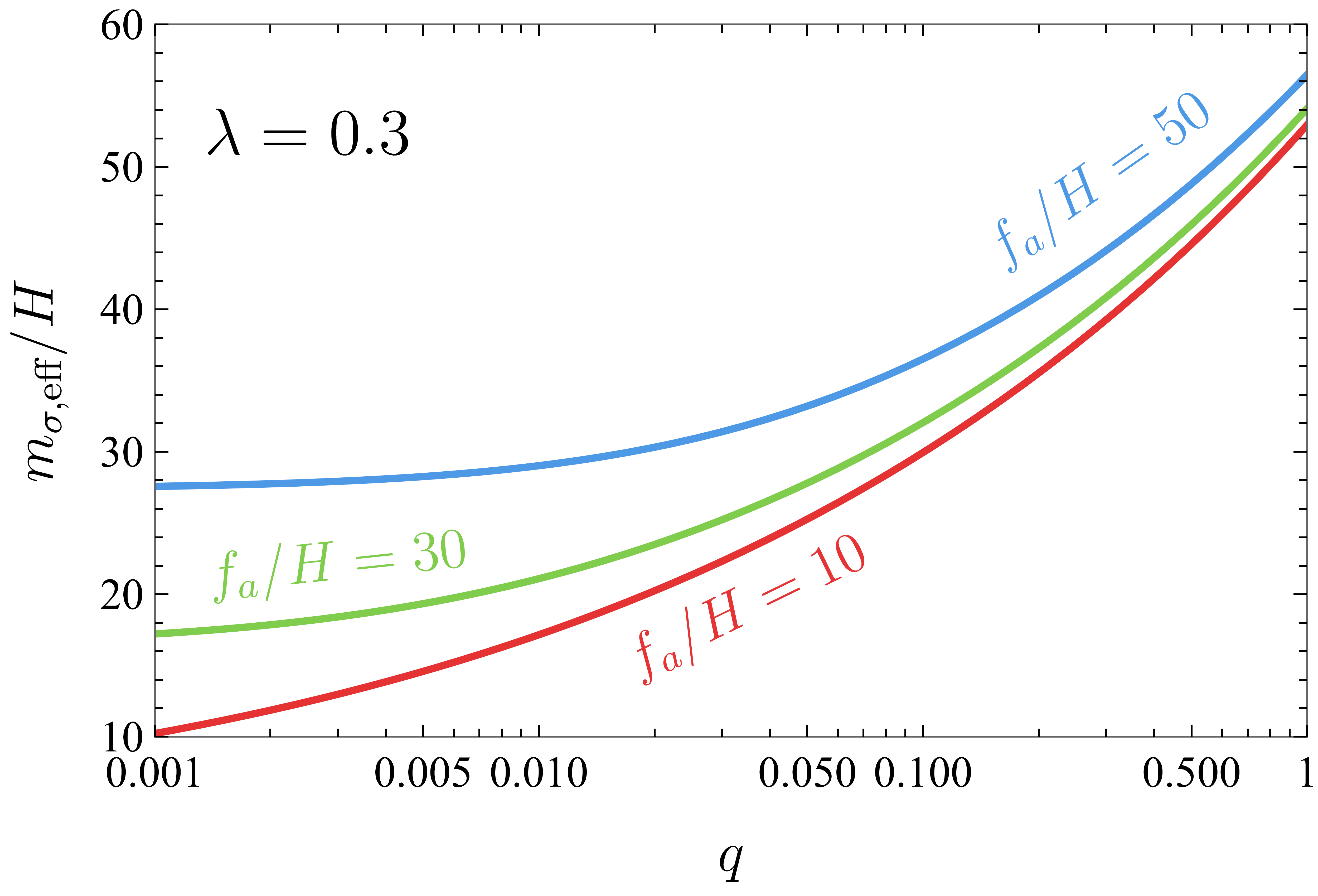
Eq. (12) and Eq. (14) allow us to solve $f_{I}/H$ and $m_{\sigma,\rm eff}/H$ as a function of $f_{a}/H,q$ and $\lambda$. For the natural value of $\lambda\sim 1$ and different choices of $f_{a}/H\subset{\cal O}(10)$, we show $m_{\sigma,\rm eff}/H$ as a function of $q$ in Fig. 1. One can see that when $q$ increases, the contribution to $m_{\sigma,\rm eff}/H$ from the inflaton-PQ field coupling dominates over that from the PQ-field potential, approaching an asymptotic value $(2\lambda)^{1/4}\sqrt{\dot{\phi}_{0}}/H$ at $q=1$. Smaller $\lambda$ allows for larger $f_{a}/H$ to achieve the same $m_{\sigma,\rm eff}/H$.

In all the models we consider, $m_{\sigma,\rm eff}=\sqrt{\lambda}f_{I}\gg H$ during inflation, the cosmological production of $\sigma$, and the induced CC signals will be exponentially suppressed by $\sim e^{-\pi m_{\sigma,\rm eff}/H}$, as mentioned in the summary of Sec. 3. To enhance the signals, we need to introduce some boosting mechanisms. In model 1 and 2, we will rely on the primordial feature mechanism in which the inflaton potential possesses a sharp feature and can be decomposed as

$$V_{\phi}=V_{\phi 0}+V_{\phi 1}~,~~|V_{\phi 1}|\ll|V_{\phi 0}|~,$$

(19)

where $V_{\phi 0}$ is the smooth potential responsible for the featureless attractor solution in Eq. (13), while the perturbation $V_{\phi 1}$ is a small sudden change of the potential localized in some regions of the field space. Then the classical background trajectories can be split into the featureless (with subscript $0$) and featured (with subscript $1$) components correspondingly:

$$\phi_{\rm bkg}(t)=\phi_{0}(t)+\phi_{1}(t)~,~~\sigma_{\rm bkg}(t)=\sigma_{0}(t)+\sigma_{1}(t)=\sigma_{1}(t)~,$$

(20)

where $\phi_{0}(t)$ is given in Eq. (13) and $\sigma_{0}(t)=0$. Note that since $a$ does not couple to the inflaton directly, $a_{\rm bkg}(t)$ is a constant.

There are many examples of sharp features. Such features can be easily envisioned when we embed the inflation models in a potential landscape when the universe is unstable. There are also motivations from CMB data analyses Peiris:2003ff; Adams:2001vc; Bean:2008na; Mortonson:2009qv; Hazra:2010ve; Hazra:2014goa; Miranda:2014fwa; Braglia:2021sun; Braglia:2021rej; Braglia:2022ftm. A sharp feature could naturally excite the classical oscillation of a massive field, such as the radial mode of the PQ field, which is otherwise hard to probe because its mass is much larger than the Hubble scale. In this paper, as a toy example, we consider $V_{\phi 1}$ to be a sharp step function:

$\displaystyle V_{\phi 1}(\phi)$

$\displaystyle=-bV_{\phi 0}\,\theta(\phi-\phi_{s})~,$

(21)

where $b\subset(0,1)$ is a dimensionless quantity; $\theta(\phi-\phi_{s})$ is the Heaviside $\theta$ function: it is one when $\phi>\phi_{s}$ and zero otherwise, which means that the perturbation potential is a small but sharp downward-step. Similar or other examples of sharp features with a more complicated form have been used to explain the CMB residual anomalies Peiris:2003ff; Adams:2001vc; Bean:2008na; Mortonson:2009qv; Hazra:2010ve; Hazra:2014goa; Miranda:2014fwa; Braglia:2021sun; Braglia:2021rej; Braglia:2022ftm. Here we just use this simplest form to illustrate the new clock and CC observables.

The time evolution of $\phi_{1}$ and $\sigma_{1}$ due to $V_{\phi 1}$ follow the equations of motion (EOMs) below:

		$\displaystyle\ddot{\phi}_{1}+3H\dot{\phi}_{1}+\left.\frac{\partial{V_{\phi 1}}(\phi)}{\partial\phi}\right|_{\phi=\phi_{0}}\simeq 0~,$		(22)
		$\displaystyle\ddot{\sigma}_{1}+3H\dot{\sigma}_{1}+\frac{cf_{I}}{\Lambda^{2}}\left(\dot{\phi}_{\rm bkg}^{2}-\dot{\phi}_{0}^{2}\right)+m_{\sigma;\rm eff}^{2}\sigma_{1}\simeq 0~$
	$\displaystyle\Rightarrow~$	$\displaystyle\ddot{\sigma}_{1}+3H\dot{\sigma}_{1}+\frac{cf_{I}}{\Lambda^{2}}\left(2\dot{\phi}_{0}\dot{\phi}_{1}\right)+m_{\sigma;\rm eff}^{2}\sigma_{1}\simeq 0~,$		(23)

where we approximate $\dot{\phi}_{\rm bkg}^{2}-\dot{\phi}_{0}^{2}\approx 2\dot{\phi}_{0}\dot{\phi}_{1}$. Given Eq. (21), the solutions are

	$\displaystyle\phi_{1}(t)$	$\displaystyle=\frac{bV_{\phi 0}}{3H\dot{\phi}_{0}}\left[1-e^{-3H(t-t_{s})}\right]\theta(t-t_{s})~,$		(24)
	$\displaystyle\sigma_{1}(t)$	$\displaystyle\simeq\frac{2c\,bV_{\phi 0}f_{I}}{\Lambda^{2}\,m^{2}_{\sigma,{\rm eff}}}\left\{e^{-\frac{3}{2}H(t-t_{s})}\cos\left[\mu_{\sigma}H(t-t_{s})\right]-e^{-3H(t-t_{s})}\right\}\theta(t-t_{s})~,$
	$\displaystyle\mu_{\sigma}$	$\displaystyle\equiv\sqrt{\frac{m^{2}_{\sigma,{\rm eff}}}{H^{2}}-\frac{9}{4}}~,$		(25)

where $t_{s}$ corresponds to the time when the inflaton passes through $\phi_{s}$ and we ignore higher-order terms suppressed by more powers of $m_{\sigma,{\rm eff}}/H\simeq\mu_{\sigma}$ in $\sigma_{1}(t)$. An illustration of this scenario is presented in Fig. 2. The inflaton velocity has a steep jump at $t=t_{s}$ with $(\dot{\phi}_{\rm bkg}^{2}-\dot{\phi}_{0}^{2})/\dot{\phi}_{0}^{2}|_{t=t_{s}}\approx{2bV_{\phi 0}}/{\dot{\phi}_{0}^{2}}$. This triggers oscillation in the radial mode $\sigma$ with an amplitude proportional to $c$ and suppressed by $m^{2}_{\sigma,{\rm eff}}$ or equivalently $\mu_{\sigma}^{2}$ when $\mu_{\sigma}\gg 1$.

References

- (1) R. D. Peccei and H. R. Quinn, CP Conservation in the Presence of Instantons, Phys. Rev. Lett. 38 (1977) 1440.
- (2) R. D. Peccei and H. R. Quinn, Constraints Imposed by CP Conservation in the Presence of Instantons, Phys. Rev. D 16 (1977) 1791.
- (3) S. Weinberg, A New Light Boson?, Phys. Rev. Lett. 40 (1978) 223.
- (4) F. Wilczek, Problem of Strong and Invariance in the Presence of Instantons, Phys. Rev. Lett. 40 (1978) 279.
- (5) J. Preskill, M. B. Wise and F. Wilczek, Cosmology of the Invisible Axion, Phys. Lett. B 120 (1983) 127.
- (6) M. Dine and W. Fischler, The Not So Harmless Axion, Phys. Lett. B 120 (1983) 137.
- (7) L. F. Abbott and P. Sikivie, A Cosmological Bound on the Invisible Axion, Phys. Lett. B 120 (1983) 133.
- (8) P. Sikivie, Axion Cosmology, Lect. Notes Phys. 741 (2008) 19 [astro-ph/0610440].
- (9) D. J. E. Marsh, Axion Cosmology, Phys. Rept. 643 (2016) 1 [1510.07633].
- (10) L. Di Luzio, M. Giannotti, E. Nardi and L. Visinelli, The landscape of QCD axion models, Phys. Rept. 870 (2020) 1 [2003.01100].
- (11) C. B. Adams et al., Axion Dark Matter, in 2022 Snowmass Summer Study, 3, 2022, 2203.14923.
- (12) P. Agrawal, K. V. Berghaus, J. Fan, A. Hook, G. Marques-Tavares and T. Rudelius, Some open questions in axion theory, in 2022 Snowmass Summer Study, 3, 2022, 2203.08026.
- (13) P. Asadi et al., Early-Universe Model Building, 2203.06680.
- (14) A. H. Guth, The Inflationary Universe: A Possible Solution to the Horizon and Flatness Problems, Phys. Rev. D 23 (1981) 347.
- (15) A. A. Starobinsky, A New Type of Isotropic Cosmological Models Without Singularity, Phys. Lett. B 91 (1980) 99.
- (16) A. D. Linde, A New Inflationary Universe Scenario: A Possible Solution of the Horizon, Flatness, Homogeneity, Isotropy and Primordial Monopole Problems, Phys. Lett. B 108 (1982) 389.
- (17) A. Albrecht and P. J. Steinhardt, Cosmology for Grand Unified Theories with Radiatively Induced Symmetry Breaking, Phys. Rev. Lett. 48 (1982) 1220.
- (18) P. J. Steinhardt and M. S. Turner, Saving the Invisible Axion, Phys. Lett. B 129 (1983) 51.
- (19) D. Seckel and M. S. Turner, Isothermal Density Perturbations in an Axion Dominated Inflationary Universe, Phys. Rev. D 32 (1985) 3178.
- (20) D. H. Lyth, A Limit on the Inflationary Energy Density From Axion Isocurvature Fluctuations, Phys. Lett. B 236 (1990) 408.
- (21) M. S. Turner and F. Wilczek, Inflationary axion cosmology, Phys. Rev. Lett. 66 (1991) 5.
- (22) A. D. Linde, Axions in inflationary cosmology, Phys. Lett. B 259 (1991) 38.
- (23) Planck collaboration, Planck 2018 results. X. Constraints on inflation, Astron. Astrophys. 641 (2020) A10 [1807.06211].
- (24) X. Chen and Y. Wang, Quasi-Single Field Inflation and Non-Gaussianities, JCAP 04 (2010) 027 [0911.3380].
- (25) N. Arkani-Hamed and J. Maldacena, Cosmological Collider Physics, 1503.08043.
- (26) X. Chen and Y. Wang, Large non-Gaussianities with Intermediate Shapes from Quasi-Single Field Inflation, Phys. Rev. D 81 (2010) 063511 [0909.0496].
- (27) D. Baumann and D. Green, Signatures of Supersymmetry from the Early Universe, Phys. Rev. D 85 (2012) 103520 [1109.0292].
- (28) V. Assassi, D. Baumann and D. Green, On Soft Limits of Inflationary Correlation Functions, JCAP 11 (2012) 047 [1204.4207].
- (29) X. Chen and Y. Wang, Quasi-Single Field Inflation with Large Mass, JCAP 09 (2012) 021 [1205.0160].
- (30) E. Sefusatti, J. R. Fergusson, X. Chen and E. P. S. Shellard, Effects and Detectability of Quasi-Single Field Inflation in the Large-Scale Structure and Cosmic Microwave Background, JCAP 08 (2012) 033 [1204.6318].
- (31) J. Norena, L. Verde, G. Barenboim and C. Bosch, Prospects for constraining the shape of non-Gaussianity with the scale-dependent bias, JCAP 08 (2012) 019 [1204.6324].
- (32) S. Pi and M. Sasaki, Curvature Perturbation Spectrum in Two-field Inflation with a Turning Trajectory, JCAP 10 (2012) 051 [1205.0161].
- (33) T. Noumi, M. Yamaguchi and D. Yokoyama, Effective field theory approach to quasi-single field inflation and effects of heavy fields, JHEP 06 (2013) 051 [1211.1624].
- (34) J.-O. Gong, S. Pi and M. Sasaki, Equilateral non-Gaussianity from heavy fields, JCAP 11 (2013) 043 [1306.3691].
- (35) R. Emami, Spectroscopy of Masses and Couplings during Inflation, JCAP 04 (2014) 031 [1311.0184].
- (36) X. Chen, M. H. Namjoo and Y. Wang, Quantum Primordial Standard Clocks, JCAP 02 (2016) 013 [1509.03930].
- (37) E. Dimastrogiovanni, M. Fasiello and M. Kamionkowski, Imprints of Massive Primordial Fields on Large-Scale Structure, JCAP 02 (2016) 017 [1504.05993].
- (38) A. Kehagias and A. Riotto, High Energy Physics Signatures from Inflation and Conformal Symmetry of de Sitter, Fortsch. Phys. 63 (2015) 531 [1501.03515].
- (39) X. Chen, Y. Wang and Z.-Z. Xianyu, Loop Corrections to Standard Model Fields in Inflation, JHEP 08 (2016) 051 [1604.07841].
- (40) H. Lee, D. Baumann and G. L. Pimentel, Non-Gaussianity as a Particle Detector, JHEP 12 (2016) 040 [1607.03735].
- (41) P. D. Meerburg, M. Münchmeyer, J. B. Muñoz and X. Chen, Prospects for Cosmological Collider Physics, JCAP 03 (2017) 050 [1610.06559].
- (42) X. Chen, Y. Wang and Z.-Z. Xianyu, Standard Model Background of the Cosmological Collider, Phys. Rev. Lett. 118 (2017) 261302 [1610.06597].
- (43) X. Chen, Y. Wang and Z.-Z. Xianyu, Standard Model Mass Spectrum in Inflationary Universe, JHEP 04 (2017) 058 [1612.08122].
- (44) X. Chen, Y. Wang and Z.-Z. Xianyu, Schwinger-Keldysh Diagrammatics for Primordial Perturbations, JCAP 12 (2017) 006 [1703.10166].
- (45) A. Kehagias and A. Riotto, On the Inflationary Perturbations of Massive Higher-Spin Fields, JCAP 07 (2017) 046 [1705.05834].
- (46) H. An, M. McAneny, A. K. Ridgway and M. B. Wise, Quasi Single Field Inflation in the non-perturbative regime, JHEP 06 (2018) 105 [1706.09971].
- (47) H. An, M. McAneny, A. K. Ridgway and M. B. Wise, Non-Gaussian Enhancements of Galactic Halo Correlations in Quasi-Single Field Inflation, Phys. Rev. D 97 (2018) 123528 [1711.02667].
- (48) A. V. Iyer, S. Pi, Y. Wang, Z. Wang and S. Zhou, Strongly Coupled Quasi-Single Field Inflation, JCAP 01 (2018) 041 [1710.03054].
- (49) S. Kumar and R. Sundrum, Heavy-Lifting of Gauge Theories By Cosmic Inflation, JHEP 05 (2018) 011 [1711.03988].
- (50) X. Chen, W. Z. Chua, Y. Guo, Y. Wang, Z.-Z. Xianyu and T. Xie, Quantum Standard Clocks in the Primordial Trispectrum, JCAP 05 (2018) 049 [1803.04412].
- (51) X. Chen, Y. Wang and Z.-Z. Xianyu, Neutrino Signatures in Primordial Non-Gaussianities, JHEP 09 (2018) 022 [1805.02656].
- (52) W. Z. Chua, Q. Ding, Y. Wang and S. Zhou, Imprints of Schwinger Effect on Primordial Spectra, JHEP 04 (2019) 066 [1810.09815].
- (53) S. Kumar and R. Sundrum, Seeing Higher-Dimensional Grand Unification In Primordial Non-Gaussianities, JHEP 04 (2019) 120 [1811.11200].
- (54) Y.-P. Wu, Higgs as heavy-lifted physics during inflation, JHEP 04 (2019) 125 [1812.10654].
- (55) A. Moradinezhad Dizgah, H. Lee, J. B. Muñoz and C. Dvorkin, Galaxy Bispectrum from Massive Spinning Particles, JCAP 05 (2018) 013 [1801.07265].
- (56) R. Saito and T. Kubota, Heavy Particle Signatures in Cosmological Correlation Functions with Tensor Modes, JCAP 06 (2018) 009 [1804.06974].
- (57) X. Tong, Y. Wang and S. Zhou, Unsuppressed primordial standard clocks in warm quasi-single field inflation, JCAP 06 (2018) 013 [1801.05688].
- (58) J. Fan, M. Reece and Y. Wang, An Inflationary Probe of Cosmic Higgs Switching, JHEP 05 (2020) 042 [1905.05764].
- (59) S. Alexander, S. J. Gates, L. Jenks, K. Koutrolikos and E. McDonough, Higher Spin Supersymmetry at the Cosmological Collider: Sculpting SUSY Rilles in the CMB, JHEP 10 (2019) 156 [1907.05829].
- (60) S. Lu, Y. Wang and Z.-Z. Xianyu, A Cosmological Higgs Collider, JHEP 02 (2020) 011 [1907.07390].
- (61) A. Hook, J. Huang and D. Racco, Searches for other vacua. Part II. A new Higgstory at the cosmological collider, JHEP 01 (2020) 105 [1907.10624].
- (62) A. Hook, J. Huang and D. Racco, Minimal signatures of the Standard Model in non-Gaussianities, Phys. Rev. D 101 (2020) 023519 [1908.00019].
- (63) S. Kumar and R. Sundrum, Cosmological Collider Physics and the Curvaton, JHEP 04 (2020) 077 [1908.11378].
- (64) L.-T. Wang and Z.-Z. Xianyu, In Search of Large Signals at the Cosmological Collider, JHEP 02 (2020) 044 [1910.12876].
- (65) T. Liu, X. Tong, Y. Wang and Z.-Z. Xianyu, Probing P and CP Violations on the Cosmological Collider, JHEP 04 (2020) 189 [1909.01819].
- (66) D.-G. Wang, On the inflationary massive field with a curved field manifold, JCAP 01 (2020) 046 [1911.04459].
- (67) Y. Wang and Y. Zhu, Cosmological Collider Signatures of Massive Vectors from Non-Gaussian Gravitational Waves, JCAP 04 (2020) 049 [2001.03879].
- (68) L. Li, S. Lu, Y. Wang and S. Zhou, Cosmological Signatures of Superheavy Dark Matter, JHEP 07 (2020) 231 [2002.01131].
- (69) L.-T. Wang and Z.-Z. Xianyu, Gauge Boson Signals at the Cosmological Collider, JHEP 11 (2020) 082 [2004.02887].
- (70) J. Fan and Z.-Z. Xianyu, A Cosmic Microscope for the Preheating Era, JHEP 01 (2021) 021 [2005.12278].
- (71) K. Kogai, K. Akitsu, F. Schmidt and Y. Urakawa, Galaxy imaging surveys as spin-sensitive detector for cosmological colliders, JCAP 03 (2021) 060 [2009.05517].
- (72) A. Bodas, S. Kumar and R. Sundrum, The Scalar Chemical Potential in Cosmological Collider Physics, JHEP 02 (2021) 079 [2010.04727].
- (73) S. Aoki and M. Yamaguchi, Disentangling mass spectra of multiple fields in cosmological collider, JHEP 04 (2021) 127 [2012.13667].
- (74) N. Arkani-Hamed, D. Baumann, H. Lee and G. L. Pimentel, The Cosmological Bootstrap: Inflationary Correlators from Symmetries and Singularities, JHEP 04 (2020) 105 [1811.00024].
- (75) D. Baumann, C. Duaso Pueyo, A. Joyce, H. Lee and G. L. Pimentel, The cosmological bootstrap: weight-shifting operators and scalar seeds, JHEP 12 (2020) 204 [1910.14051].
- (76) D. Baumann, C. Duaso Pueyo, A. Joyce, H. Lee and G. L. Pimentel, The Cosmological Bootstrap: Spinning Correlators from Symmetries and Factorization, SciPost Phys. 11 (2021) 071 [2005.04234].
- (77) N. Maru and A. Okawa, Non-Gaussianity from gauge bosons in Cosmological Collider Physics, 2101.10634.
- (78) S. Lu, Axion isocurvature collider, JHEP 04 (2022) 157 [2103.05958].
- (79) Q. Lu, M. Reece and Z.-Z. Xianyu, Missing scalars at the cosmological collider, JHEP 12 (2021) 098 [2108.11385].
- (80) L.-T. Wang, Z.-Z. Xianyu and Y.-M. Zhong, Precision calculation of inflation correlators at one loop, JHEP 02 (2022) 085 [2109.14635].
- (81) X. Tong, Y. Wang and Y. Zhu, Cutting rule for cosmological collider signals: a bulk evolution perspective, JHEP 03 (2022) 181 [2112.03448].
- (82) L. Pinol, S. Aoki, S. Renaux-Petel and M. Yamaguchi, Inflationary flavor oscillations and the cosmic spectroscopy, Phys. Rev. D 107 (2023) L021301 [2112.05710].
- (83) Y. Cui and Z.-Z. Xianyu, Probing Leptogenesis with the Cosmological Collider, Phys. Rev. Lett. 129 (2022) 111301 [2112.10793].
- (84) X. Tong and Z.-Z. Xianyu, Large spin-2 signals at the cosmological collider, JHEP 10 (2022) 194 [2203.06349].
- (85) M. Reece, L.-T. Wang and Z.-Z. Xianyu, Large-Field Inflation and the Cosmological Collider, 2204.11869.
- (86) G. L. Pimentel and D.-G. Wang, Boostless cosmological collider bootstrap, JHEP 10 (2022) 177 [2205.00013].
- (87) Z. Qin and Z.-Z. Xianyu, Phase information in cosmological collider signals, JHEP 10 (2022) 192 [2205.01692].
- (88) X. Chen, R. Ebadi and S. Kumar, Classical cosmological collider physics and primordial features, JCAP 08 (2022) 083 [2205.01107].
- (89) S. Jazayeri and S. Renaux-Petel, Cosmological bootstrap in slow motion, JHEP 12 (2022) 137 [2205.10340].
- (90) D. Ghosh, A. H. Singh and F. Ullah, Probing the initial state of inflation: analytical structure of cosmological correlators, 2207.06430.
- (91) Z. Qin and Z.-Z. Xianyu, Helical Inflation Correlators: Partial Mellin-Barnes and Bootstrap Equations, 2208.13790.
- (92) Z.-Z. Xianyu and H. Zhang, Bootstrapping One-Loop Inflation Correlators with the Spectral Decomposition, 2211.03810.
- (93) X. Niu, M. H. Rahat, K. Srinivasan and W. Xue, Gravitational wave probes of massive gauge bosons at the cosmological collider, JCAP 02 (2023) 013 [2211.14331].
- (94) X. Niu, M. H. Rahat, K. Srinivasan and W. Xue, Parity-Odd and Even Trispectrum from Axion Inflation, 2211.14324.
- (95) D.-G. Wang, G. L. Pimentel and A. Achúcarro, Bootstrapping Multi-Field Inflation: non-Gaussianities from light scalars revisited, 2212.14035.
- (96) S. Aoki, Continuous Spectrum on Cosmological Collider, 2301.07920.
- (97) D. Werth, L. Pinol and S. Renaux-Petel, Cosmological Flow of Primordial Correlators, 2302.00655.
- (98) WMAP collaboration, First year Wilkinson Microwave Anisotropy Probe (WMAP) observations: Implications for inflation, Astrophys. J. Suppl. 148 (2003) 213 [astro-ph/0302225].
- (99) J. A. Adams, B. Cresswell and R. Easther, Inflationary perturbations from a potential with a step, Phys. Rev. D 64 (2001) 123514 [astro-ph/0102236].
- (100) R. Bean, X. Chen, G. Hailu, S. H. H. Tye and J. Xu, Duality Cascade in Brane Inflation, JCAP 03 (2008) 026 [0802.0491].
- (101) M. J. Mortonson, C. Dvorkin, H. V. Peiris and W. Hu, CMB polarization features from inflation versus reionization, Phys. Rev. D 79 (2009) 103519 [0903.4920].
- (102) D. K. Hazra, M. Aich, R. K. Jain, L. Sriramkumar and T. Souradeep, Primordial features due to a step in the inflaton potential, JCAP 10 (2010) 008 [1005.2175].
- (103) D. K. Hazra, A. Shafieloo, G. F. Smoot and A. A. Starobinsky, Wiggly Whipped Inflation, JCAP 08 (2014) 048 [1405.2012].
- (104) V. Miranda, W. Hu and C. Dvorkin, Polarization Predictions for Inflationary CMB Power Spectrum Features, Phys. Rev. D 91 (2015) 063514 [1411.5956].
- (105) M. Braglia, X. Chen and D. K. Hazra, Uncovering the history of cosmic inflation from anomalies in cosmic microwave background spectra, Eur. Phys. J. C 82 (2022) 498 [2106.07546].
- (106) M. Braglia, X. Chen and D. K. Hazra, Primordial standard clock models and CMB residual anomalies, Phys. Rev. D 105 (2022) 103523 [2108.10110].
- (107) M. Braglia, X. Chen, D. K. Hazra and L. Pinol, Back to the features: assessing the discriminating power of future CMB missions on inflationary models, 2210.07028.
- (108) X. Chen, Primordial Non-Gaussianities from Inflation Models, Adv. Astron. 2010 (2010) 638979 [1002.1416].
- (109) J. Chluba, J. Hamann and S. P. Patil, Features and New Physical Scales in Primordial Observables: Theory and Observation, Int. J. Mod. Phys. D 24 (2015) 1530023 [1505.01834].
- (110) A. Slosar et al., Scratches from the Past: Inflationary Archaeology through Features in the Power Spectrum of Primordial Fluctuations, Bull. Am. Astron. Soc. 51 (2019) 98 [1903.09883].
- (111) X. Chen, Primordial Features as Evidence for Inflation, JCAP 01 (2012) 038 [1104.1323].
- (112) X. Chen, Fingerprints of Primordial Universe Paradigms as Features in Density Perturbations, Phys. Lett. B 706 (2011) 111 [1106.1635].
- (113) X. Chen and C. Ringeval, Searching for Standard Clocks in the Primordial Universe, JCAP 08 (2012) 014 [1205.6085].
- (114) T. Battefeld, J. C. Niemeyer and D. Vlaykov, Probing Two-Field Open Inflation by Resonant Signals in Correlation Functions, JCAP 05 (2013) 006 [1302.3877].
- (115) X. Gao, D. Langlois and S. Mizuno, Oscillatory features in the curvature power spectrum after a sudden turn of the inflationary trajectory, JCAP 10 (2013) 023 [1306.5680].
- (116) T. Noumi and M. Yamaguchi, Primordial spectra from sudden turning trajectory, JCAP 12 (2013) 038 [1307.7110].
- (117) R. Saito, M. Nakashima, Y.-i. Takamizu and J. Yokoyama, Resonant Signatures of Heavy Scalar Fields in the Cosmic Microwave Background, JCAP 11 (2012) 036 [1206.2164].
- (118) R. Saito and Y.-i. Takamizu, Localized Features in Non-Gaussianity from Heavy Physics, JCAP 06 (2013) 031 [1303.3839].
- (119) X. Chen and M. H. Namjoo, Standard Clock in Primordial Density Perturbations and Cosmic Microwave Background, Phys. Lett. B 739 (2014) 285 [1404.1536].
- (120) X. Chen, M. H. Namjoo and Y. Wang, Models of the Primordial Standard Clock, JCAP 02 (2015) 027 [1411.2349].
- (121) Q.-G. Huang and S. Pi, Power-law modulation of the scalar power spectrum from a heavy field with a monomial potential, JCAP 04 (2018) 001 [1610.00115].
- (122) G. Domènech, J. Rubio and J. Wons, Mimicking features in alternatives to inflation with interacting spectator fields, Phys. Lett. B 790 (2019) 263 [1811.08224].
- (123) M. Braglia, X. Chen and D. K. Hazra, Comparing multi-field primordial feature models with the Planck data, JCAP 06 (2021) 005 [2103.03025].
- (124) A. Bodas and R. Sundrum, Primordial clocks within stochastic gravitational wave anisotropies, JCAP 10 (2022) 012 [2205.04482].
- (125) M. Kawasaki, K. Nakayama, T. Sekiguchi, T. Suyama and F. Takahashi, Non-Gaussianity from isocurvature perturbations, JCAP 11 (2008) 019 [0808.0009].
- (126) C. Hikage, M. Kawasaki, T. Sekiguchi and T. Takahashi, CMB constraint on non-Gaussianity in isocurvature perturbations, JCAP 07 (2013) 007 [1211.1095].
- (127) G. W. Gibbons and S. W. Hawking, Cosmological Event Horizons, Thermodynamics, and Particle Creation, Phys. Rev. D 15 (1977) 2738.
- (128) M. P. Hertzberg, M. Tegmark and F. Wilczek, Axion Cosmology and the Energy Scale of Inflation, Phys. Rev. D 78 (2008) 083507 [0807.1726].
- (129) M. Dine, P. Draper, L. Stephenson-Haskins and D. Xu, Axions, Instantons, and the Lattice, Phys. Rev. D 96 (2017) 095001 [1705.00676].
- (130) J. Martin and L. Pinol, Opening the reheating box in multifield inflation, JCAP 12 (2021) 022 [2105.03301].
- (131) G. Lazarides, R. K. Schaefer, D. Seckel and Q. Shafi, Dilution of Cosmological Axions by Entropy Production, Nucl. Phys. B 346 (1990) 193.
- (132) M. Kawasaki, T. Moroi and T. Yanagida, Can decaying particles raise the upper bound on the Peccei-Quinn scale?, Phys. Lett. B 383 (1996) 313 [hep-ph/9510461].
- (133) T. Banks and M. Dine, The Cosmology of string theoretic axions, Nucl. Phys. B 505 (1997) 445 [hep-th/9608197].
- (134) G. F. Giudice, E. W. Kolb and A. Riotto, Largest temperature of the radiation era and its cosmological implications, Phys. Rev. D 64 (2001) 023508 [hep-ph/0005123].
- (135) D. Grin, T. L. Smith and M. Kamionkowski, Axion constraints in non-standard thermal histories, Phys. Rev. D 77 (2008) 085020 [0711.1352].
- (136) K. V. Berghaus and T. Karwal, Thermal Friction as a Solution to the Hubble Tension, Phys. Rev. D 101 (2020) 083537 [1911.06281].
- (137) A. Papageorgiou, P. Quílez and K. Schmitz, Axion dark matter from frictional misalignment, JHEP 01 (2023) 169 [2206.01129].
- (138) K. Choi, S. H. Im, H. J. Kim and H. Seong, Axion dark matter with thermal friction, JHEP 02 (2023) 180 [2206.01462].
- (139) I. J. Allali, M. P. Hertzberg and Y. Lyu, Reduced axion abundance from an extended symmetry, Phys. Rev. D 107 (2023) 043535 [2211.07661].
- (140) I. J. Allali, M. P. Hertzberg and Y. Lyu, Altered axion abundance from a dynamical Peccei-Quinn scale, Phys. Rev. D 105 (2022) 123517 [2203.15817].
- (141) L. Li, T. Nakama, C. M. Sou, Y. Wang and S. Zhou, Gravitational Production of Superheavy Dark Matter and Associated Cosmological Signatures, JHEP 07 (2019) 067 [1903.08842].
- (142) C. M. Sou, X. Tong and Y. Wang, Chemical-potential-assisted particle production in FRW spacetimes, JHEP 06 (2021) 129 [2104.08772].
- (143) Y. Bao, J. Fan and L. Li, Opening up window of post-inflationary QCD axion, 2209.09908.
- (144) P. Creminelli, On non-Gaussianities in single-field inflation, JCAP 10 (2003) 003 [astro-ph/0306122].
- (145) X. Chen, R. Easther and E. A. Lim, Generation and Characterization of Large Non-Gaussianities in Single Field Inflation, JCAP 04 (2008) 010 [0801.3295].
- (146) R. Flauger, L. McAllister, E. Pajer, A. Westphal and G. Xu, Oscillations in the CMB from Axion Monodromy Inflation, JCAP 06 (2010) 009 [0907.2916].
- (147) R. Flauger and E. Pajer, Resonant Non-Gaussianity, JCAP 01 (2011) 017 [1002.0833].
- (148) X. Chen, Folded Resonant Non-Gaussianity in General Single Field Inflation, JCAP 12 (2010) 003 [1008.2485].
- (149) “Axion limits on fa.” https://github.com/cajohare/AxionLimits/blob/master/plots/Axion_fa.pdf.
- (150) A. Achúcarro et al., Inflation: Theory and Observations, 2203.08128.
- (151) Z. Huang, L. Verde and F. Vernizzi, Constraining inflation with future galaxy redshift surveys, JCAP 04 (2012) 005 [1201.5955].
- (152) D. K. Hazra, Changes in the halo formation rates due to features in the primordial spectrum, JCAP 03 (2013) 003 [1210.7170].
- (153) X. Chen, C. Dvorkin, Z. Huang, M. H. Namjoo and L. Verde, The Future of Primordial Features with Large-Scale Structure Surveys, JCAP 11 (2016) 014 [1605.09365].
- (154) M. Ballardini, F. Finelli, C. Fedeli and L. Moscardini, Probing primordial features with future galaxy surveys, JCAP 10 (2016) 041 [1606.03747].
- (155) G. A. Palma, D. Sapone and S. Sypsas, Constraints on inflation with LSS surveys: features in the primordial power spectrum, JCAP 06 (2018) 004 [1710.02570].
- (156) B. L’Huillier, A. Shafieloo, D. K. Hazra, G. F. Smoot and A. A. Starobinsky, Probing features in the primordial perturbation spectrum with large-scale structure data, Mon. Not. Roy. Astron. Soc. 477 (2018) 2503 [1710.10987].
- (157) M. Ballardini, F. Finelli, R. Maartens and L. Moscardini, Probing primordial features with next-generation photometric and radio surveys, JCAP 04 (2018) 044 [1712.07425].
- (158) F. Beutler, M. Biagetti, D. Green, A. Slosar and B. Wallisch, Primordial Features from Linear to Nonlinear Scales, Phys. Rev. Res. 1 (2019) 033209 [1906.08758].
- (159) M. Ballardini, R. Murgia, M. Baldi, F. Finelli and M. Viel, Non-linear damping of superimposed primordial oscillations on the matter power spectrum in galaxy surveys, JCAP 04 (2020) 030 [1912.12499].
- (160) I. Debono, D. K. Hazra, A. Shafieloo, G. F. Smoot and A. A. Starobinsky, Constraints on features in the inflationary potential from future Euclid data, Mon. Not. Roy. Astron. Soc. 496 (2020) 3448 [2003.05262].
- (161) Y. Li, H.-M. Zhu and B. Li, Non-linear reconstruction of features in the primordial power spectrum from large-scale structure, Mon. Not. Roy. Astron. Soc. 514 (2022) 4363 [2102.09007].
- (162) M. Ballardini, F. Finelli, F. Marulli, L. Moscardini and A. Veropalumbo, New constraints on primordial features from the galaxy two-point correlation function, 2202.08819.
- (163) D. Chandra and S. Pal, Investigating the constraints on primordial features with future cosmic microwave background and galaxy surveys, JCAP 09 (2022) 024 [2205.01164].
- (164) X. Chen, P. D. Meerburg and M. Münchmeyer, The Future of Primordial Features with 21 cm Tomography, JCAP 09 (2016) 023 [1605.09364].
- (165) Y. Xu, J. Hamann and X. Chen, Precise measurements of inflationary features with 21 cm observations, Phys. Rev. D 94 (2016) 123518 [1607.00817].
- (166) J. Fumagalli, S. Renaux-Petel and L. T. Witkowski, Oscillations in the stochastic gravitational wave background from sharp features and particle production during inflation, JCAP 08 (2021) 030 [2012.02761].
- (167) M. Braglia, X. Chen and D. K. Hazra, Probing Primordial Features with the Stochastic Gravitational Wave Background, JCAP 03 (2021) 005 [2012.05821].
- (168) X. Chen, R. Easther and E. A. Lim, Large Non-Gaussianities in Single Field Inflation, JCAP 06 (2007) 023 [astro-ph/0611645].
- (169) P. Adshead, C. Dvorkin, W. Hu and E. A. Lim, Non-Gaussianity from Step Features in the Inflationary Potential, Phys. Rev. D 85 (2012) 023531 [1110.3050].
- (170) D. K. Hazra, L. Sriramkumar and J. Martin, BINGO: A code for the efficient computation of the scalar bi-spectrum, JCAP 05 (2013) 026 [1201.0926].
- (171) N. Bartolo, D. Cannone and S. Matarrese, The Effective Field Theory of Inflation Models with Sharp Features, JCAP 10 (2013) 038 [1307.3483].
- (172) J. R. Fergusson, H. F. Gruetjen, E. P. S. Shellard and M. Liguori, Combining power spectrum and bispectrum measurements to detect oscillatory features, Phys. Rev. D 91 (2015) 023502 [1410.5114].
- (173) J. R. Fergusson, H. F. Gruetjen, E. P. S. Shellard and B. Wallisch, Polyspectra searches for sharp oscillatory features in cosmic microwave sky data, Phys. Rev. D 91 (2015) 123506 [1412.6152].
- (174) M. Freytsis, S. Kumar, G. N. Remmen and N. L. Rodd, Multifield Positivity Bounds for Inflation, 2210.10791.
- (175) Planck collaboration, Planck 2018 results. IX. Constraints on primordial non-Gaussianity, Astron. Astrophys. 641 (2020) A9 [1905.05697].
- (176) J. E. Kim, Weak Interaction Singlet and Strong CP Invariance, Phys. Rev. Lett. 43 (1979) 103.
- (177) M. A. Shifman, A. I. Vainshtein and V. I. Zakharov, Can Confinement Ensure Natural CP Invariance of Strong Interactions?, Nucl. Phys. B 166 (1980) 493.
- (178) K. S. Jeong and F. Takahashi, Suppressing Isocurvature Perturbations of QCD Axion Dark Matter, Phys. Lett. B 727 (2013) 448 [1304.8131].
- (179) K. Choi, K. S. Jeong and M.-S. Seo, String theoretic QCD axions in the light of PLANCK and BICEP2, JHEP 07 (2014) 092 [1404.3880].
- (180) E. J. Chun, Axion Dark Matter with High-Scale Inflation, Phys. Lett. B 735 (2014) 164 [1404.4284].
- (181) M. Fairbairn, R. Hogan and D. J. E. Marsh, Unifying inflation and dark matter with the Peccei-Quinn field: observable axions and observable tensors, Phys. Rev. D 91 (2015) 023509 [1410.1752].
- (182) K. Nakayama and M. Takimoto, Higgs inflation and suppression of axion isocurvature perturbation, Phys. Lett. B 748 (2015) 108 [1505.02119].
- (183) K. Harigaya, M. Ibe, M. Kawasaki and T. T. Yanagida, Dynamics of Peccei-Quinn Breaking Field after Inflation and Axion Isocurvature Perturbations, JCAP 11 (2015) 003 [1507.00119].
- (184) J. Kearney, N. Orlofsky and A. Pierce, High-Scale Axions without Isocurvature from Inflationary Dynamics, Phys. Rev. D 93 (2016) 095026 [1601.03049].