An Online Algorithm for Chance constrained Resource Allocation

Consider the multi-dimensional RAP with $n$ requests and $m$ resources. For each request, there are always $k$ resource consumption schemes that can satisfy it. When a request is revealed, the decision maker chooses one scheme or none. Without loss of generality, a deterministic multi-dimensional RAP can be modeled as follows:

where the revenue coefficient vector $\bm{c}_{t}\in\mathbb{R}^{k}$, and the resource consumption vector $\bm{a}_{tj}\in\mathbb{R}^{k}$. The decision variables are $(\bm{x}_{1},\dots,\bm{x}_{n})$. $x_{tl}=1$ means that $t$-th request is satisfied by resource consumption scheme $l$. $b_{j}$ is the capacity of resource $j$. $\bm{1}$ denotes all-one vector. In the online setting of ILP, the input data $(\bm{c}_{t},\bm{a}_{t1},\dots,\bm{a}_{tm})$ is revealed one by one and $\bm{x}_{t}$ is determined instantaneously when $(\bm{c}_{t},\bm{a}_{t1},\dots,\bm{a}_{tm})$ is revealed without future information. Moreover, $n$ and $\bm{b}$ is known and fixed before the first input arrives.

In practical, the value of $\bm{a}_{tj}$ can be obtained by prediction which yields the uncertainty. Consequently, taken the uncertainty of $\bm{a}_{tj}$ into consideration, we formulate the following CCP problem:

where $\mathbb{P}$ means probability and $\eta_{j}$ is the given confidence level. Assume that the true value of $\bm{a}_{tj}$ belongs to a known Gaussian distribution with mean $\bar{\bm{a}}_{tj}$ and covariance matrix $\bm{K}_{tj}$ [26], and then problem (2) is equivalent to the following deterministic problem [27]:

where $\Phi(\cdot)$ represents the cumulative distribution function of the standard Gaussian distribution. Moreover, when $\bm{a}_{tj}$ follows a distribution with a finite support, which need not to be Gaussian distribution, problem (2) can also be translated into the same form in (3) according to the previous work [28]. Problem (3) is an integer second-order cone programming (ISOCP) problem when $\eta_{j}>50\%,\forall j$. The offline ISOCP problems can be solved by commercial solvers such as Gurobi. However, in the online setting, it is difficult to solve problem (3) due to its non-linearity: $\bm{x}_{t}$ with different subscripts t are coupled with each other in $({\sum_{t=1}^{n}\bm{x}_{t}^{\top}\bm{K}_{tj}\bm{x}_{t}})^{1/2}$. In the online setting of CCP, the input data is $(\bm{c}_{t},\bar{\bm{a}}_{t1},\dots,\bar{\bm{a}}_{tm},\bm{K}_{t1},\dots,\bm{K}_{tm})$.

To address the non-decomposable issue raised by the non-linearity of $\sqrt{\sum_{t=1}^{n}\bm{x}_{t}^{\top}\bm{K}_{tj}\bm{x}_{t}}$, we linearize this term to decouple different $\bm{x}_{t}$. Specifically, according to Cauchy-Schwarz inequality $\sqrt{n\sum_{t=1}^{n}\bm{x}_{t}^{\top}\bm{K}_{tj}\bm{x}_{t}}\geq\sum_{t=1}^{n}\sqrt{\bm{x}_{t}^{\top}\bm{K}_{tj}\bm{x}_{t}}$ and Proposition 1, the nonlinear problem (3) can be approximated by

Problem (4) is linear and can be solved in the online setting. The online algorithm for solving this relaxed problem is the basis of our algorithm for solving the CCP problem (3) and we will detail it in the following section.

Recall that (4) is an ILP problem and Li et al. [11] have proposed an effective OPD algorithm to solve the online ILP problem. For simplicity, denote $\tilde{\bm{a}}_{tj}=\bar{\bm{a}}_{tj}+{\Phi^{-1}(\eta_{j})}\bm{\gamma}_{tj}{/\sqrt{n}}$ and we present the OPD method as shown in Algorithm 1.

In Algorithm 1, denote $\tilde{\bm{A}}_{t}=(\tilde{\bm{a}}_{t1}^{\top},\dots,\tilde{\bm{a}}_{tm}^{\top})^{\top}$ and $\bm{b}=(b_{1},\dots,b_{m})^{\top}$. Algorithm 1 is dual-based which maintains a dual vector $\bm{p}_{t}$. In each iteration, new $\bm{c}_{t}$ and $\tilde{\bm{A}}_{t}$ are revealed. Then, $\bm{x}_{t}$ is determined by choosing $l$ that maximizes $(\bm{c}_{t}^{\top}-\bm{p}_{t}^{\top}\tilde{\bm{A}}_{t})\bm{e}_{l}$, where $\bm{e}_{l}$ is the unit vector with all components equal to 0 except the $l$-th, which is 1. After determining $\bm{x}_{t}$, $\bm{p}_{t}$ is updated by a projected stochastic subgradient descent method where $(\bm{d}-\tilde{\bm{A}}_{t}\bm{x}_{t})$ is the subgradient corresponding to $\bm{p}_{t}$.

The following Theorem 1 states that Algorithm 1 achieves $O(\sqrt{n})$ regret and constraint violation compared to the optimal solution of the ISOCP problem (3). The detailed proof of Theorem 1 as well as Proposition 1 is presented in the full-length version [29].

Although Algorithm 1 has been able to obtain a near-optimal solution of the ISOCP problem (3) according to Theorem 1, its practical performance can be further improved by narrowing the gap between the solutions generated by Algorithm 1 and the offline ISOCP (3). To be specific, this gap mainly comes from the following two points:

1. (a)

   The error between the offline ILP problem (4) and the offline ISOCP problem (3).

2. (b)

   The error between the online solution and offline solution of the ILP problem (4).

To address these issues, we propose the modified OPD Algorithm 2 for solving the online CCP problem (3). In Algorithm 2, several heuristic corrections are applied to correct the above-mentioned errors.

First is to correct the error (a). For the $j$-th constraint, we introduce scale factors

to reduce the gap between $\sqrt{\sum_{t=1}^{n}\bm{x}_{t}^{\top}\bm{K}_{tj}\bm{x}_{t}}$ and $\sum_{t=1}^{n}{\bm{\gamma}_{tj}^{\top}\bm{x}_{t}}$ $/{\sqrt{n}}$. Next, we define $\hat{\bm{a}}_{t1}(\beta_{tj})=\bar{\bm{a}}_{tj}+\beta_{tj}{\Phi^{-1}(\eta_{j})}{}\bm{\gamma}_{tj}/\sqrt{n}$ and $\hat{\bm{A}}_{t}(\bm{\beta_{t}})$ = $(\hat{\bm{a}}_{t1}^{\top}(\beta_{t1}),\dots,\hat{\bm{a}}_{tm}^{\top}(\beta_{tm}))^{\top}.$ In Algorithm 2, $\hat{\bm{A}}_{t}(\bm{\beta_{t}})$ is used in place of $\tilde{\bm{A}}_{t}$. That is, we use $\sum_{t=1}^{n}\beta_{tj}\bm{\gamma}_{tj}^{\top}\bm{x}_{t}/\sqrt{n}$ to approximate $\sqrt{\sum_{t=1}^{n}\bm{x}_{t}^{\top}\bm{K}_{tj}\bm{x}_{t}}$. At time $t$, $\bm{\beta}_{t}$ is calculated according to (7) which is based on the historical decisions and will be used in the next iteration for correction. It is worth noting that $\bm{\beta}_{t}=(\beta_{t1},\dots,\beta_{tm})^{\top}$ is calculated in each round and can be computed incrementally with low computational cost.

In the numerical experiments section 4, it is illustrated that Algorithm 2 has better performance than Algorithm 1 in terms of the constraint violation. An intuitive explanation is that Algorithm 2 is more inclined to reject the orders with high uncertainty of resource consumption (i.e., $\bm{K}_{tj}$) than Algorithm 1 because $\bm{\beta}_{t}\geq\bm{1}$.

Next is to correct the error (b). The error (b) consists of two parts, the optimality gap and constraint violation. The constraint violation will cause the probability $\mathbb{P}\left(\sum\nolimits_{t=1}^{n}\bm{a}_{tj}^{\top}\bm{x}_{t}\leq b_{j}\right)$ to deviate from the target value $\eta_{j}$. It is almost impossible to reduce the optimality gap and probability deviation simultaneously. Compared with the optimality gap, the CCP problems have a lower tolerance for the probability deviation. In order to reduce the probability deviation, we propose the following method to dynamically adjust the right-hand-side capacity $\bm{d}$ in each iteration:

The intuition behind the correction formula (8) is given as follows: if too many resources are spent in the early rounds, the average remaining resources $\bm{d}$ will diminish. Then Algorithm 2 will raise the dual price and be more likely to reject an order with high resource consumption as a result. On the other hand, if a large number of orders with high resource consumption are rejected at the start, resulting in an excess of remaining resources, Algorithm 2 will decrease the dual price in order to accept more orders in the future. This correction strategy makes Algorithm 2 perform better than Algorithms 1 in numerical experiments.

In the first experiment, we set $k=5$ and $m=4$. The confidence levels of chance constraints are set to (0.65, 0.75, 0.85, 0.95). For each value of $n$, we run 20 simulation trials. In each trial, coefficients $\bm{c}_{tj}$, $\bm{\bar{a}}_{tj}$ and $\bm{K}_{tj}$ are resampled.

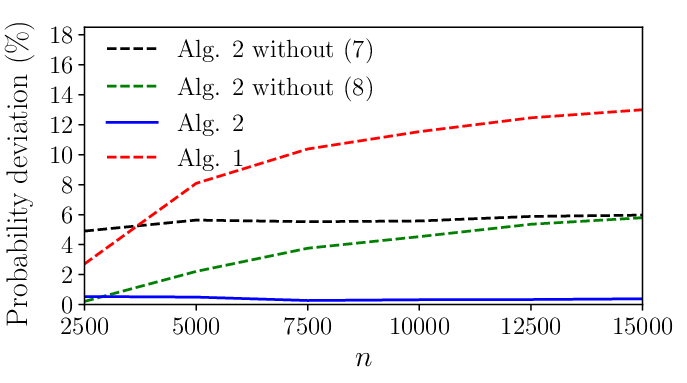
Fig. 1 shows the average optimality gap and probability deviation over all the simulation trials. The probability deviation of the whole problem in one trail is an average:

where $\bm{x}_{t}$ is the output of the algorithms. The calculation formula for the expected optimality gap is (5). From Fig. 1, we observe that the optimality gaps of these algorithms are close and Algorithm 2 has the smallest probability deviation. Fig. 1 (a) also shows that the optimality gap of Algorithm 2 is on the order of $\sqrt{n}$. Fig. 2 presents the probability deviations of each chance constraint of Algorithm 1 and 2. Fig. 1 and 2 both illustrate that the proposed two corrections (7) and (8) can effectively reduce the probability deviation with minor negative effects on the optimality gap.

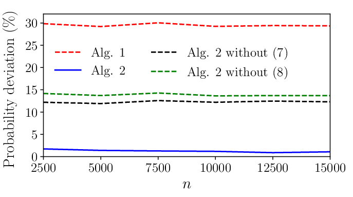
In the second experiment, $k$ and $m$ are still set to 5 and 4. The confidence levels are also the same as those in Experiment I. For each value of $n$, we run 20 simulation trials. In each trial, coefficients $\bm{c}_{tj}$, $\bm{\bar{a}}_{tj}$ and $\bm{K}_{tj}$ are i.i.d. sampled from Chi-square distributions which are unbounded.

Fig. 3 shows the average optimality gap and probability deviation, and Fig. 4 shows the probability deviations of each chance constraint of Algorithm 1 and 2. The results of Experiment II are similar to those of Experiment I: Algorithm 2 has the smallest probability deviation; corrections (7) and (8) can effectively reduce the probability deviation. Although Algorithm 2 produces slightly larger optimality gap, its optimality gap is still approximately on the order of $\sqrt{n}$. In this experiment with unbounded input, Algorithm 2 has obvious advantages: the probability deviations of the algorithms except Algorithm 2 are larger than 10%, while the probability deviation of Algorithm 2 is less than 1%.

In addition, the competitive ratios of Algorithm 2 in Experiment I and II are not less than 96%, with details provided in this doc [30].

In the following, we present an engineering application of our method in the task of order fulfillment based on the real data obtained from Cainiao Network which is a supply chain company. The request (order) is revealed one by one, and the algorithm needs to decide which transportation channel the order will be sent to. $x_{tl}=1$ denotes the order $t$ is sent to channel $l$. The objective coefficient is the revenue of each channel and the constraint coefficient is the predicted transportation time of each channel. The deterministic problem is to maximize the total revenue while ensuring that the average transportation time is not larger than 15 working days. The transportation time is obtained from prediction which introduces the uncertainty in the constraint coefficients. We adopt the chance constraint with the holding probability of average transportation time $\geq 90\%$. Due to that each order must be assigned to a channel, the constraint $\bm{1}^{\top}\bm{x}_{t}\leq 1$ in (2) is replaced with $\bm{1}^{\top}\bm{x}_{t}=1$ and Algorithms are also slightly modified accordingly: do not judge whether $v_{t}>0$ and always set $\bm{x}_{t}=\bm{e}_{l_{t}}$. Three different transportation channels are considered. The simulation results are shown blow.

The above results also show that Algorithm 2 with proposed corrections is effective for reducing the value of the probability deviation while not sacrificing the optimality gap too much.

References

- [1] Arash Asadpour, Xuan Wang, and Jiawei Zhang, “Online resource allocation with limited flexibility,” Management Science, vol. 66, no. 2, pp. 642–666, 2020.
- [2] David A. Schmidt, Changxin Shi, Randall A. Berry, Michael L. Honig, and Wolfgang Utschick, “Distributed resource allocation schemes,” IEEE Signal Processing Magazine, vol. 26, no. 5, pp. 53–63, 2009.
- [3] James F. Kurose and Rahul Simha, “A microeconomic approach to optimal resource allocation in distributed computer systems,” IEEE Transactions on Computers, vol. 38, no. 5, pp. 705–717, 1989.
- [4] Masaaki Ida, “Portfolio selection problem with interval coefficients,” Applied Mathematics Letters, vol. 16, no. 5, pp. 709–713, 2003.
- [5] Marco Molinaro and Ramamoorthi Ravi, “The geometry of online packing linear programs,” Mathematics of Operations Research, vol. 39, no. 1, pp. 46–59, 2014.
- [6] Xiaocheng Li and Yinyu Ye, “Online linear programming: Dual convergence, new algorithms, and regret bounds,” Operations Research, 2021.
- [7] Shipra Agrawal, Zizhuo Wang, and Yinyu Ye, “A dynamic near-optimal algorithm for online linear programming,” Operations Research, vol. 62, no. 4, pp. 876–890, 2014.
- [8] Anupam Gupta and Marco Molinaro, “How experts can solve lps online,” in European Symposium on Algorithms. Springer, 2014, pp. 517–529.
- [9] Xiao Alison Chen and Zizhuo Wang, “A dynamic learning algorithm for online matching problems with concave returns,” European Journal of Operational Research, vol. 247, no. 2, pp. 379–388, 2015.
- [10] Wenzhi Gao, Chunlin Sun, Yuyang Ye, and Yinyu Ye, “Boosting method in approximately solving linear programming with fast online algorithm,” arXiv preprint arXiv:2107.03570, 2021.
- [11] Xiaocheng Li, Chunlin Sun, and Yinyu Ye, “Simple and fast algorithm for binary integer and online linear programming,” in Advances in Neural Information Processing Systems, 2020, pp. 9412–9421.
- [12] Santiago R Balseiro, Haihao Lu, and Vahab Mirrokni, “Dual mirror descent for online allocation problems,” in International Conference on Machine Learning. PMLR, 2020, pp. 613–628.
- [13] Santiago R Balseiro, Haihao Lu, and Vahab Mirrokni, “The best of many worlds: Dual mirror descent for online allocation problems,” Operations Research, 2022.
- [14] Russell Bent and Pascal Van Hentenryck, “Online stochastic and robust optimization,” in Annual Asian Computing Science Conference. Springer, 2004, pp. 286–300.
- [15] Russell Bent and Pascal Van Hentenryck, “Online stochastic optimization without distributions,” in Proceedings of the Fifteenth International Conference on International Conference on Automated Planning and Scheduling. 2005, pp. 171–180, AAAI Press.
- [16] Jiashuo Jiang, Xiaocheng Li, and Jiawei Zhang, “Online stochastic optimization with wasserstein based non-stationarity,” arXiv preprint arXiv:2012.06961, 2020.
- [17] Jialin Liu, Yuantao Gu, and Mengdi Wang, “Averaging random projection: A fast online solution for large-scale constrained stochastic optimization,” in IEEE ICASSP. IEEE, 2015, pp. 3586–3590.
- [18] Jiashuo Jiang and Jiawei Zhang, “Online resource allocation with stochastic resource consumption,” arXiv preprint arXiv:2012.07933, 2020.
- [19] Abraham Charnes and William W Cooper, “Chance-constrained programming,” Management Science, vol. 6, no. 1, pp. 73–79, 1959.
- [20] Andrzej Ruszczyński and Alexander Shapiro, “Stochastic programming models,” Handbooks in Operations Research and Management Science, vol. 10, pp. 1–64, 2003.
- [21] András Prékopa, Stochastic programming, vol. 324, Springer Science & Business Media, 2013.
- [22] Raj Jagannathan, “Chance-constrained programming with joint constraints,” Operations Research, vol. 22, no. 2, pp. 358–372, 1974.
- [23] Abraham Charnes and William W Cooper, “Deterministic equivalents for optimizing and satisficing under chance constraints,” Operations Research, vol. 11, no. 1, pp. 18–39, 1963.
- [24] Andras Prekopa, “Contributions to the theory of stochastic programming,” Mathematical Programming, vol. 4, no. 1, pp. 202–221, 1973.
- [25] Pu Li, Harvey Arellano-Garcia, and Günter Wozny, “Chance constrained programming approach to process optimization under uncertainty,” Computers & Chemical Engineering, vol. 32, no. 1-2, pp. 25–45, 2008.
- [26] F. Hosseinzadeh Lotfi, N. Nematollahi, M.H. Behzadi, M. Mirbolouki, and Z. Moghaddas, “Centralized resource allocation with stochastic data,” Journal of Computational and Applied Mathematics, vol. 236, no. 7, pp. 1783–1788, 2012.
- [27] Stephen Boyd and Lieven Vandenberghe, Convex Optimization, pp. 237–238, Cambridge University Press, 2004.
- [28] Maxime C Cohen, Philipp W Keller, Vahab Mirrokni, and Morteza Zadimoghaddam, “Overcommitment in cloud services: Bin packing with chance constraints,” Management Science, vol. 65, no. 7, pp. 3255–3271, 2019.
- [29] Yuwei Chen, Zengde Deng, Zaiyi Chen, Yinzhi Zhou, Yujie Chen, and Haoyuan Hu, “Online primal-dual algorithms for stochastic resource allocation problems,” arXiv preprint arXiv:2203.16818, 2022.
- [30] Yuwei Chen and Zengde Deng, “Experiment results,” 2022, Google Drive https://docs.google.com/spreadsheets/d/11-gPDpoai704BtRPJgJFRNMUMoO4iNZ_/.