跳到论文正文
W Papers独立论文阅读器 arXiv:2303.02889 论文正文 计算阅读时间 · 0%
引用这篇论文根据当前论文元数据生成,正式投稿前建议核对。


License: arXiv.org perpetual non-exclusive license
arXiv:2303.02889v1 [math.GT] 06 Mar 2023

Surface gluing with signs and gradings in decategorified Heegaard Floer theory

Andrew Manion Address: Department of Mathematics, North Carolina State University, 2108 SAS Hall, Raleigh, NC 27695 Email address: ajmanion@ncsu.edu
Abstract.

A previous result about the decategorified bordered (sutured) Heegaard Floer invariants of surfaces glued together along intervals, generalizing the decategorified content of Rouquier and the author’s higher-tensor-product-based gluing theorem in cornered Heegaard Floer homology, was proved only over 𝔽2\mathbb{F}_{2} and without gradings. In this paper we add signs and prove a graded version of the interval gluing theorem over ℤ\mathbb{Z}, enabling a more detailed comparison of these aspects of decategorified Heegaard Floer theory with modern work on non-semisimple 3d TQFTs in mathematics and physics.

1. Introduction

In [MR20], Raphaël Rouquier and the author reformulated and extended work of Douglas–Manolescu [DM14] to prove a more structured gluing theorem for the algebras that bordered sutured Heegaard Floer homology [LOT18, Zar11] assigns to surfaces. The gluing theorem of [MR20] is based on a new tensor product construction for higher representations of a particular dg monoidal category [Kho14] related to 𝔤​𝔩​(1|1)+\mathfrak{gl}(1|1)^{+}. Given such a gluing theorem, it is natural to look for a TQFT interpretation. Some preliminary remarks to this end, focusing on the connection with 2d open-closed cobordisms, appear in [MR20, Section 7.2.5].

More can be said once one passes from the full version of bordered sutured Heegaard Floer theory to its decategorification, in which the higher tensor products become ordinary tensor products of representations of a Hopf algebra. Indeed, in [Man22], the author proved a gluing theorem for decategorified bordered sutured Heegaard Floer invariants of surfaces, generalizing the decategorification of the gluing theorem from [MR20] and placing it in a more flexible and TQFT-like setting. However, the results of [Man22] were only formulated and proved without gradings and with coefficients in 𝔽2\mathbb{F}_{2}, where one can ignore plus and minus signs (this was reasonable in relationship with [MR20] where the grading structure does not readily lead to a decategorification over ℤ\mathbb{Z}).

One reason to add gradings and signs to the results of [Man22] is to bring decategorified bordered sutured Heegaard Floer theory more in line with the recently active area of non-semisimple 3d TQFT [ADO92, CGPM14, Mik15, BCGPM16, GPV17, AGPS18, GPPV20, GHN+21, CGP21, Jag22, GY22], especially the theory called 𝔭​𝔰​𝔩​(1|1)\mathfrak{psl}(1|1) Chern–Simons theory by Mikhaylov [Mik15] and whose homological truncation is given a proposed mathematical description in Geer–Young’s 𝒟q,int\mathcal{D}^{q,\intt} TQFT for generic qq [GY22]. Based on the connection between Heegaard Floer homology and 𝔤​𝔩​(1|1)\mathfrak{gl}(1|1), as explained from a unified perspective in [GPV17, Section 3.3], one hopes that ideas from decategorified bordered sutured Heegaard Floer theory can advance the study of these non-semisimple 3d TQFTs and vice-versa. However, it is difficult to compare these TQFTs with [Man22] directly; they are defined over ℂ\mathbb{C} rather than 𝔽2\mathbb{F}_{2}, and gradings are a key aspect of [Mik15, GY22] but are absent in [Man22]. See [CGP21, Section 5] for a discussion of the important role played by gradings in non-semisimple 3d TQFT in general.

The main result of this paper is a version with gradings and signs of the generalized gluing theorem from [Man22]. To state it, let 2Cobext\Cob^{\ext} denote Lauda–Pfeiffer’s open-closed cobordism category [LP08]; informally, objects MM of 2Cobext\Cob^{\ext} are disjoint unions of oriented circles and intervals, and morphisms are 2d open-closed cobordisms. If F:M1→M2F\colon M_{1}\to M_{2} is such a morphism, we will write11 1 As mentioned in [MR20, Man22] and reviewed below, a morphism F:M1→M2F\colon M_{1}\to M_{2} in 2Cobext\Cob^{\ext} can be canonically identified with a sutured surface (F,Λ,S+,S−)(F,\Lambda,S_{+},S_{-}) in the sense of Zarev [Zar11, Definition 1.2], allowing closed components of FF as well as components of ∂F\partial F that are disjoint from Λ\Lambda and contained fully in S+S_{+} or S−S_{-}, and equipped with a partition of S+S_{+} into “source” M1M_{1} and “target” M2M_{2} along with an ordering of the components of MiM_{i} for i∈{1,2}i\in\{1,2\}. S+=M2⊔(−M1)S_{+}=M_{2}\sqcup(-M_{1}) for the subset of ∂F\partial F corresponding to the source M1M_{1} and target M2M_{2} of FF. For an object MM of 2Cobext\Cob^{\ext} we will write A⁡(M)A(M) for the tensor product, over all interval components of MM, of ℤ\mathbb{Z}-graded22 2 In general, when considering ℤ\mathbb{Z}- or ℚ\mathbb{Q}-graded super abelian groups in this paper, we will not let the grading affect the signs in symmetrizers; only the parity as a super abelian group will contribute. super rings ℤ⁡[E]/(E2)=Uℤ​(𝔤​𝔩​(1|1)+)\mathbb{Z}[E]/(E^{2})=U^{\mathbb{Z}}(\mathfrak{gl}(1|1)^{+}) (one for each interval component) where EE is odd and has ℤ\mathbb{Z}-degree −1-1.

Let F:M1→M2F\colon M_{1}\to M_{2} be a morphism in 2Cobext\Cob^{\ext} (we think of M1M_{1} as being on the right and M2M_{2} as being on the left). The decategorification over 𝔽2\mathbb{F}_{2} of Zarev’s bordered sutured Heegaard Floer invariant of FF is isomorphic to ∧∗H1(F,S+;𝔽2)\wedge^{*}H_{1}(F,S_{+};\mathbb{F}_{2}). If we let A𝔽2​(Mi):=A⁡(Mi)⊗ℤ𝔽2A^{\mathbb{F}_{2}}(M_{i}):=A(M_{i})\otimes_{\mathbb{Z}}\mathbb{F}_{2}, then decategorifying the higher actions of [MR20] gives ∧∗H1(F,S+;𝔽2)\wedge^{*}H_{1}(F,S_{+};\mathbb{F}_{2}) the structure of a bimodule over (A𝔽2​(M2),A𝔽2​(M1))(A^{\mathbb{F}_{2}}(M_{2}),A^{\mathbb{F}_{2}}(M_{1})) as shown in [Man22], and we get a functor

∧∗H1(F,S+;𝔽2)⊗A𝔽2​(M1)−\wedge^{*}H_{1}(F,S_{+};\mathbb{F}_{2})\otimes_{A^{\mathbb{F}_{2}}(M_{1})}-

from the category of left modules over A𝔽2​(M1)A^{\mathbb{F}_{2}}(M_{1}) to the category of left modules over A𝔽2​(M2)A^{\mathbb{F}_{2}}(M_{2}). For a composition of morphisms in 2Cobext\Cob^{\ext} that only involves gluing along intervals and not circles, by [Man22, Theorem 1.3] the bimodule or functor associated to the glued surface is a tensor product or composition of the bimodules or functors associated to the two pieces.

Over ℤ\mathbb{Z} we will consider the ℚ\mathbb{Q}-graded33 3 When choosing the function δ:𝒮→ℚ\delta\colon\mathcal{S}\to\mathbb{Q} below, one could decide to incorporate arbitrarily complicated fractions, or even real or complex numbers after changing the codomain of δ\delta, into its definition. However, the most motivated choices appear to involve only simple fractions like half-integers and (1/4)(1/4)-integers when they involve fractions at all, and if one sticks to such choices then elements of ℚ\mathbb{Q} with arbitrarily complicated denominators will not appear. super abelian groups

𝐙δ,πS+(F):=(ℤ0|1)⊗π⁡(F)⊗∧∗H1(F,S+;ℤ){δ(F)}\mathbf{Z}^{S_{+}}_{\delta,\pi}(F):=\left(\mathbb{Z}^{0|1}\right)^{\otimes\pi(F)}\otimes\wedge^{*}H_{1}(F,S_{+};\mathbb{Z})\{\delta(F)\}

(homology coefficients will be ℤ\mathbb{Z} unless otherwise stated) where:

  • •

    ℤ0|1\mathbb{Z}^{0|1} denotes ℤ\mathbb{Z} as a purely odd super abelian group concentrated in ℚ\mathbb{Q}-degree zero;

  • •

    the exterior algebra without shifts lives in ℚ\mathbb{Q}-degrees 0,1,…,h0,1,\ldots,h where

    h:=rank⁡H1​(F,S+)h:=\rk H_{1}(F,S_{+})

    (see equation (9) below for a combinatorial formula for hh);

  • •

    δ:𝒮→ℚ\delta\colon\mathcal{S}\to\mathbb{Q} and π:𝒮→ℤ/2​ℤ\pi\colon\mathcal{S}\to\mathbb{Z}/2\mathbb{Z}, where 𝒮\mathcal{S} is the set of sutured surfaces, are “degree-shift” and “parity” functions on 𝒮\mathcal{S}, chosen from a parametrized family Π\Pi of such functions that we will describe below;

  • •

    the brackets {⋅}\{\cdot\} denote an upward shift of the ℚ\mathbb{Q}-degree by the enclosed quantity.

We will define the structure of a bimodule over (A⁡(M2),A⁡(M1))(A(M_{2}),A(M_{1})) on 𝐙δ,πS+​(F)\mathbf{Z}^{S_{+}}_{\delta,\pi}(F).

Remark 1.1.

We want to think of the parity shift as being mediated by an explicit prefactor (ℤ0|1)⊗π⁡(F)\left(\mathbb{Z}^{0|1}\right)^{\otimes\pi(F)} that appears on one side of ∧∗H1(F,S+)\wedge^{*}H_{1}(F,S_{+}) or the other, rather than just an abstract shift like [π⁡(F)][\pi(F)], because to make the signs work out in the gluing theorem, odd algebra elements trying to act on ∧∗H1(F,S+)\wedge^{*}H_{1}(F,S_{+}) should pick up a sign or not based on whether they need to commute past the prefactor.

Theorem 1.2.

Let M1M_{1}, M2M_{2}, and M3M_{3} be objects of 2Cobext\Cob^{\ext}, and assume that M2M_{2} has only intervals and no circles. Let

M3←F′M2←𝐹M1M_{3}\xleftarrow{F^{\prime}}M_{2}\xleftarrow{F}M_{1}

be morphisms in 2Cobext\Cob^{\ext}. For any choice in the family Π\Pi of a pair (δ,π)(\delta,\pi), we have

𝐙δ,πS+​(F′∘F)≅𝐙δ,πS+​(F′)⊗A⁡(M2)𝐙δ,πS+​(F)\mathbf{Z}^{S_{+}}_{\delta,\pi}(F^{\prime}\circ F)\cong\mathbf{Z}^{S_{+}}_{\delta,\pi}(F^{\prime})\otimes_{A(M_{2})}\mathbf{Z}^{S_{+}}_{\delta,\pi}(F)

as bimodules over (A⁡(M3),A⁡(M1))(A(M_{3}),A(M_{1})).

We will use Theorem 1.2 to deduce the following corollary.

Corollary 1.3.

Let 2Cobopenext\Cob^{\ext}_{\open} denote the full symmetric monoidal subcategory of 2Cobext\Cob^{\ext} on objects consisting only of intervals and no circles. For any (δ,π)∈Π(\delta,\pi)\in\Pi, the assignments M↦A⁡(M)M\mapsto A(M) and F↦𝐙δ,πS+​(F)F\mapsto\mathbf{Z}^{S_{+}}_{\delta,\pi}(F) give a symmetric monoidal functor 𝐙δ,πS+\mathbf{Z}^{S_{+}}_{\delta,\pi} from 2Cobopenext\Cob^{\ext}_{\open} to the symmetric monoidal category SAlgℤ\SAlg_{\mathbb{Z}} of ℤ\mathbb{Z}-graded super rings and ℚ\mathbb{Q}-graded bimodules up to isomorphism.

We briefly describe the family Π\Pi of degree and parity shift functions, postponing a more detailed explanation until Section 4. For a sutured surface FF with h:=rank⁡H1​(F,S+)h:=\rk H_{1}(F,S_{+}), and for any (A1,A2,A3,A4)∈ℚ4(A_{1},A_{2},A_{3},A_{4})\in\mathbb{Q}^{4}, define

(1) δA1,A2,A3,A4​(F):=\displaystyle\delta_{A_{1},A_{2},A_{3},A_{4}}(F):= −A1​h+(A1−1)​#​{no-​S+​ non-closed components of ​F}\displaystyle-A_{1}h+(A_{1}-1)\#\{\textrm{no-}S_{+}\textrm{ non-closed components of }F\}
+A2​#​{no-​S−​ non-closed components of ​F}\displaystyle+A_{2}\#\{\textrm{no-}S_{-}\textrm{ non-closed components of }F\}
+A3​#​{closed components of ​F}+((A1−1)/2)​#​{S+​ intervals}\displaystyle+A_{3}\#\{\textrm{closed components of }F\}+((A_{1}-1)/2)\#\{S_{+}\textrm{ intervals}\}
+A4​#​{S+​ circles}.\displaystyle+A_{4}\#\{S_{+}\textrm{ circles}\}.

For any (N1,N2,N3,N4)∈{0,1}4(N_{1},N_{2},N_{3},N_{4})\in\{0,1\}^{4}, define

(2) πN1,N2,N3,N4​(F)\displaystyle\pi_{N_{1},N_{2},N_{3},N_{4}}(F) =h+N1​#​{no-​S−​ non-closed components of ​F}\displaystyle=h+N_{1}\#\{\textrm{no-}S_{-}\textrm{ non-closed components of }F\}
+N2​#​{closed components of ​F}+N3​#​{S+​ intervals}\displaystyle+N_{2}\#\{\textrm{closed components of }F\}+N_{3}\#\{S_{+}\textrm{ intervals}\}
+N4​#​{S+​ circles}\displaystyle+N_{4}\#\{S_{+}\textrm{ circles}\}

modulo 2. Note that both δA1,A2,A3,A4\delta_{A_{1},A_{2},A_{3},A_{4}} and πN1,N2,N3,N4\pi_{N_{1},N_{2},N_{3},N_{4}} are additive under disjoint unions of sutured surfaces. An arbitrary element (δA1,A2,A3,A4,πN1,N2,N3,N4)(\delta_{A_{1},A_{2},A_{3},A_{4}},\pi_{N_{1},N_{2},N_{3},N_{4}}) of Π\Pi is specified by the choice of (A1,A2,A3,A4)(A_{1},A_{2},A_{3},A_{4}) and (N1,N2,N3,N4)(N_{1},N_{2},N_{3},N_{4}), which may be unrelated to each other.

Refer to caption
Figure 1. Open pp-tuple of pants 𝒫\mathcal{P}, with pp intervals on its right side and one on its left side.
Example 1.4.

To the open pp-tuple of pants 𝒫\mathcal{P} with p≥0p\geq 0 intervals in its input boundary (see Figure 1), we can ask which choices (δA1,A2,A3,A4,πN1,N2,N3,N4)∈Π(\delta_{A_{1},A_{2},A_{3},A_{4}},\pi_{N_{1},N_{2},N_{3},N_{4}})\in\Pi result in 𝒫\mathcal{P} being assigned (ℤ⁡[E]/(E2))⊗p(\mathbb{Z}[E]/(E^{2}))^{\otimes p} as a right module over itself, with left action of ℤ⁡[E]/(E2)\mathbb{Z}[E]/(E^{2}) given by iterating the coproduct

Δ⁡(E)=E⊗1+1⊗E\Delta(E)=E\otimes 1+1\otimes E

(or the counit ε⁡(E)=0\varepsilon(E)=0 when p=0p=0). Note that if this identification holds, then taking

𝐙δA1,A2,A3,A4,πN1,N2,N3,N4S+(𝒫)⊗(ℤ⁡[E]/(E2))⊗p(X1⊗ℤ⋯⊗ℤXp)\mathbf{Z}^{S_{+}}_{\delta_{A_{1},A_{2},A_{3},A_{4}},\pi_{N_{1},N_{2},N_{3},N_{4}}}(\mathcal{P})\otimes_{(\mathbb{Z}[E]/(E^{2}))^{\otimes p}}(X_{1}\otimes_{\mathbb{Z}}\cdots\otimes_{\mathbb{Z}}X_{p})

for left modules XiX_{i} over A⁡(M1)A(M_{1}) yields the tensor product X1⊗ℤ⋯⊗ℤXpX_{1}\otimes_{\mathbb{Z}}\cdots\otimes_{\mathbb{Z}}X_{p} in the monoidal category of representations of the Hopf superalgebra ℤ⁡[E]/(E2)\mathbb{Z}[E]/(E^{2}), in line with the higher-tensor-product interpretation of the gluing theorem in [MR20].

For 𝒫\mathcal{P} we have h=ph=p; the one component of 𝒫\mathcal{P} is non-closed and intersects both S+S_{+} and S−S_{-} nontrivially. It has p+1p+1 intervals in S+S_{+} and no circles in S+S_{+}. We get

δA1,A2,A3,A4(𝒫)=−pA1+((A1−1)/2)(p+1)=−p(A1+1)/2+(A1−1)/2\delta_{A_{1},A_{2},A_{3},A_{4}}(\mathcal{P})=-pA_{1}+((A_{1}-1)/2)(p+1)=-p(A_{1}+1)/2+(A_{1}-1)/2

and

πN1,N2,N3,N4​(𝒫)=p+N3​(p+1).\pi_{N_{1},N_{2},N_{3},N_{4}}(\mathcal{P})=p+N_{3}(p+1).

It will turn out (see Proposition 2.7) that we want the basis element of ∧∗H1(𝒫,S+)\wedge^{*}H_{1}(\mathcal{P},S_{+}) in the highest degree to correspond to ±1∈(ℤ⁡[E]/(E2))⊗p\pm 1\in(\mathbb{Z}[E]/(E^{2}))^{\otimes p}. Thus, we want δA1,A2,A3,A4​(𝒫)=−p\delta_{A_{1},A_{2},A_{3},A_{4}}(\mathcal{P})=-p and (modulo 2) πN1,N2,N3,N4​(𝒫)=p\pi_{N_{1},N_{2},N_{3},N_{4}}(\mathcal{P})=p. For any choice of parameters with

A1=1andN3=0,A_{1}=1\quad\textrm{and}\quad N_{3}=0,

we get a grading shift that recovers tensor products in Rep⁡(ℤ⁡[E]/(E2))\Rep(\mathbb{Z}[E]/(E^{2})) from the open pair of pants 𝒫\mathcal{P} for all pp. The choice (A1,A2,A3,A4)=(1,0,0,0)(A_{1},A_{2},A_{3},A_{4})=(1,0,0,0) and (N1,N2,N3,N4)=(0,0,0,0)(N_{1},N_{2},N_{3},N_{4})=(0,0,0,0) stands out as particularly simple; for general FF we have

δ1,0,0,0​(F):=−handπ0,0,0,0​(F)=h.\delta_{1,0,0,0}(F):=-h\quad\textrm{and}\quad\pi_{0,0,0,0}(F)=h.

If we are only concerned with the case p=1p=1 (the identity cobordism on an interval) and not general pp, then no conditions are required on (A1,A2,A3,A4)(A_{1},A_{2},A_{3},A_{4}) and (N1,N2,N3,N4)(N_{1},N_{2},N_{3},N_{4}) for this identity cobordism to get assigned ℤ⁡[E]/(E2)\mathbb{Z}[E]/(E^{2}) as a bimodule over itself.

Remark 1.5.

As with the 𝔽2\mathbb{F}_{2} case in [Man22], the super abelian groups 𝐙δ,πS+​(F)\mathbf{Z}^{S_{+}}_{\delta,\pi}(F) do not seem to admit an analogue of Theorem 1.2 when gluing along circles rather than intervals. Relatedly, while 𝐙δ,πS+​(F)\mathbf{Z}^{S_{+}}_{\delta,\pi}(F) has actions of Uℤ​(𝔤​𝔩​(1|1)+)=ℤ⁡[E]/(E2)U^{\mathbb{Z}}(\mathfrak{gl}(1|1)^{+})=\mathbb{Z}[E]/(E^{2}) for interval components of S+S_{+}, it does not seem to have interesting actions of anything related to the full 𝔤​𝔩​(1|1)\mathfrak{gl}(1|1) (with both odd generators EE and FF of 𝔤​𝔩​(1|1)\mathfrak{gl}(1|1) acting) given a circle component of S+S_{+}. In [Man], we plan to address both limitations by introducing larger variants 𝐙δ,πP​(F)\mathbf{Z}^{P}_{\delta,\pi}(F) of the spaces 𝐙δ,πS+​(F)\mathbf{Z}^{S_{+}}_{\delta,\pi}(F) such that 𝐙δ,πP​(F)\mathbf{Z}^{P}_{\delta,\pi}(F) admits interesting actions of U⁡(𝔭​𝔰​𝔩​(1|1))U(\mathfrak{psl}(1|1)) for circle components of S+S_{+} as well as U⁡(𝔭​𝔰​𝔩​(1|1)+)U(\mathfrak{psl}(1|1)^{+}) for interval components of S+S_{+}. The spaces 𝐙δ,πP​(F)\mathbf{Z}^{P}_{\delta,\pi}(F) will satisfy analogues of Theorem 1.2 when gluing along circles as well as intervals.

Comparing with 3d non-semisimple TQFT. Consider a connected sutured surface F=Fg,pF=F_{g,p} of genus gg with p≥1p\geq 1 boundary circles in S+S_{+} and no other boundary (so S−=∅S_{-}=\varnothing). We have h=2​g−1+ph=2g-1+p. Since ∂Fg,p=S+\partial F_{g,p}=S_{+}, we have

H1​(F,S+)=H1​(F,∂F)≅H1​(F);H_{1}(F,S_{+})=H_{1}(F,\partial F)\cong H^{1}(F);

in this section on the comparison with non-semisimple TQFT, but not elsewhere, we will work over ℂ\mathbb{C} and by H1​(F)H^{1}(F) we mean H1​(F,ℂ)H^{1}(F;\mathbb{C}).

In [Mik15, Section 5.2.2], Mikhaylov looks at this sutured surface Fg,pF_{g,p} with the boundary circles viewed as punctures and labeled by line operators L𝐭𝐢,niL_{\mathbf{t_{i}},n_{i}}. He assumes that the parameters 𝐭𝐢∈ℂ×\mathbf{t_{i}}\in\mathbb{C}^{\times} are “generic,” i.e. not equal to 11 (but that their product is equal to 11), and that the parameters nin_{i} are integers. The parameters 𝐭𝐢\mathbf{t_{i}} (along with some choice of 2​g2g additional holonomies in ℂ×\mathbb{C}^{\times} when g>0g>0) specify a nontrivial complex line bundle ℒ\mathcal{L} with flat connection on Fg,pF_{g,p}. Mikhaylov sets

hgen=2​g−2+p=dimH1​(Fg,p,ℒ)h_{\gen}=2g-2+p=\dim H^{1}(F_{g,p};\mathcal{L})

(Mikhaylov calls this quantity hh but to avoid confusion we will reserve hh for the dimension of H1​(F,S+)H_{1}(F,S_{+}), which is 2​g−1+p=hgen+12g-1+p=h_{\gen}+1 in this case). The reason the dimension hgenh_{\gen} for generic holonomies 𝐭𝐢\mathbf{t_{i}} is one less than our dimension hh is the relation shown graphically in [Mik15, Figure 2]. Mikhaylov describes the 3d 𝔭​𝔰​𝔩​(1|1)\mathfrak{psl}(1|1) Chern–Simons TQFT as having state space

(detH1(Fg,p;ℒ))⊗(−1/2+N/hgen)⊗∧∗H1(Fg,p;ℒ)(\det H^{1}(F_{g,p};\mathcal{L}))^{\otimes(-1/2+N/h_{\gen})}\otimes\wedge^{*}H^{1}(F_{g,p};\mathcal{L})

on Fg,pF_{g,p} decorated by ℒ\mathcal{L}, where N=∑i=1p(−1/2+ni)N=\sum_{i=1}^{p}(-1/2+n_{i}). See [Mik15, equation (5.6)]. He gives the graded superdimension of this space as

(3) tN(t1/2−t−1/2)hgent^{N}(t^{1/2}-t^{-1/2})^{h_{\gen}}

(see [Mik15, equation (5.8)]) where powers of tt correspond to our ℚ\mathbb{Q}-grading on the state space, i.e. Mikhaylov’s U​(1)flU(1)_{\mathrm{fl}} charge.

Geer–Young note in [GY22, Section 6.1] that, in their 𝒟q,int\mathcal{D}^{q,\intt} TQFT, their graded dimension formula [GY22, equation (19)] for the Hilbert spaces of generic surfaces agrees with Mikhaylov’s formula (3), at least up to the sign in front. More explicitly, when labeling the pp boundary components of Fg,pF_{g,p} by the representations V​(αi,ni)0¯V(\alpha_{i},n_{i})_{\overline{0}} defined in [GY22, Section 2.3.2], and setting N=∑i(ni−1/2)N=\sum_{i}(n_{i}-1/2) as in Mikhaylov’s paper, Geer–Young’s equation (19) gives the graded dimension of the state space as

(4) (−1)g−1tN(t1/2−t−1/2)hgen(-1)^{g-1}t^{N}(t^{1/2}-t^{-1/2})^{h_{\gen}}

where we write Geer–Young’s qβq^{\beta} as t−1/2t^{-1/2} (see [GY22, Theorem 3.5]), and we take tμ=1t^{\mu}=1 because the product of the 𝐭𝐢\mathbf{t_{i}} is 11.

It is natural to ask how the graded super dimensions of our spaces compare with the above formulas, for various choices of degree shift and parity functions (δ,π)∈Π(\delta,\pi)\in\Pi. Our spaces are based on H1​(F,ℂ)H^{1}(F;\mathbb{C}) which arises when taking ℒ\mathcal{L} to be the trivial local system, so we will take the limit 𝐭i→1\mathbf{t}_{i}\to 1 in Mikhaylov’s analysis (and correspondingly αi→0\alpha_{i}\to 0 in Geer–Young) without worrying about possible subtleties involved with these limits as mentioned in [Mik15, Section 5.3.5]. In other words, we will be concerned with the state spaces of non-generic or critical surfaces rather than generic surfaces.

If all of Mikhaylov’s 𝐭𝐢\mathbf{t_{i}} are 11, the relation in [Mik15, Figure 2] gets trivialized. Where the graded dimension formulas in the generic case have hgenh_{\gen}, we should have hh instead. We will also take all the labels nin_{i} to be zero, so that the punctures are each labeled by V​(0,0)0¯V(0,0)_{\overline{0}}; naively extrapolating (4) leads to

(5) (−1)g−1t−p/2(t1/2−t−1/2)h.(-1)^{g-1}t^{-p/2}(t^{1/2}-t^{-1/2})^{h}.

Observations about circle gluing from a follow-up paper [Man] in preparation suggest that because we are in the non-generic case we should actually multiply (5) by −t1/2-t^{1/2} and try to recover the graded dimension formula

(6) (−1)gt−p/2+1/2(t1/2−t−1/2)h.(-1)^{g}t^{-p/2+1/2}(t^{1/2}-t^{-1/2})^{h}.

For now, note that in (6) as well as the generic formulas (3) and (4), all powers of tt are integral, but this is not true in (5). We want to characterize which choices of our parameters recover the graded dimension formula (6).

  • •

    To recover (6), we want to choose parameters so that our degree shift δA1,A2,A3,A4​(Fg,p)\delta_{A_{1},A_{2},A_{3},A_{4}}(F_{g,p}) equals

    −p/2+1/2−(1/2)(2g−1+p)=−h/2−p/2+1/2.-p/2+1/2-(1/2)(2g-1+p)=-h/2-p/2+1/2.

    Thus, we should set

    A1=1/2,A2=1/2,A4=−1/2A_{1}=1/2,\quad A_{2}=1/2,\quad A_{4}=-1/2

    with A3A_{3} left free to vary. Note that the condition A1=1/2A_{1}=1/2 is inconsistent with the condition A1=1A_{1}=1 from Example 1.4. This is one reason we chose to look at a parametrized family of grading shifts in this paper rather than singling out one shift as the canonical choice, since we view both tensor products from open pp-tuples of pants and connections to 3d non-semisimple TQFT as important in this theory.

  • •

    To recover (6), we also want our parity π⁡(Fg,p)\pi(F_{g,p}) to be

    g+(2​g−1+p)=g+p=h/2+p/2−1/2.g+(2g-1+p)=g+p=h/2+p/2-1/2.

    Since the formulas for our parity functions πN1,N2,N3,N4\pi_{N_{1},N_{2},N_{3},N_{4}} all have a coefficient of 11 rather than 1/21/2 in front of hh, there is no choice of N1N_{1} that works. However, from the perspective of [Man] it will be natural to take

    (A1,A2,A3,A4)=(1/2, 1/2, 0,−1/2)(A_{1},A_{2},A_{3},A_{4})=(1/2,\,1/2,\,0,\,-1/2)

    in (1), defining (for general open-closed cobordisms FF) a shift

    δ1/2​(F)=\displaystyle\delta_{1/2}(F)= −h/2−(1/2)#{no-S+ non-closed components of F}\displaystyle-h/2-(1/2)\#\{\textrm{no-}S_{+}\textrm{ non-closed components of }F\}
    +(1/2)​#​{no-​S−​ non-closed components of ​F}\displaystyle+(1/2)\#\{\textrm{no-}S_{-}\textrm{ non-closed components of }F\}
    −(1/4)​#​{S+​ intervals}−(1/2)​#​{S+​ circles}.\displaystyle-(1/4)\#\{S_{+}\textrm{ intervals}\}-(1/2)\#\{S_{+}\textrm{ circles}\}.

    When the number of S+S_{+} intervals of FF is equal modulo 4 to twice the number of boundary components of FF intersecting S−S_{-} nontrivially, one can show that δ1/2​(F)\delta_{1/2}(F) is an integer, so we can let

    π1/2​(F)=δ1/2​(F)modulo ​2.\pi_{1/2}(F)=\delta_{1/2}(F)\quad\textrm{modulo }2.

    For F=Fg,pF=F_{g,p} we have no S+S_{+} intervals and no boundary components of FF intersecting S−S_{-} nontrivially, so π1/2​(Fg,p)\pi_{1/2}(F_{g,p}) makes sense and we have

    π1/2(Fg,p)=−h/2−p/2+1/2.\pi_{1/2}(F_{g,p})=-h/2-p/2+1/2.

    This quantity equals h/2+p/2−1/2h/2+p/2-1/2 modulo 22, so we see that the degree shift δ1/2\delta_{1/2} and parity π1/2\pi_{1/2} combine to recover the graded dimension formula (6).

Conjecture 1.6.

When applying the Geer–Young TQFT 𝐙G​Y\mathbf{Z}^{GY} to the surface Fg,pF_{g,p} for p≥1p\geq 1, assume we are viewing all boundary components of Fg,pF_{g,p} as punctures labeled by V​(0,0)0¯V(0,0)_{\overline{0}}. View the state space 𝐙G​Y​(Fg,p)\mathbf{Z}^{GY}(F_{g,p}) as ℤ\mathbb{Z}-graded by the second ℤ\mathbb{Z} factor of Geer–Young’s grading by Z=ℤ×ℤ×ℤ/2​ℤZ=\mathbb{Z}\times\mathbb{Z}\times\mathbb{Z}/2\mathbb{Z}. For the degree-shift and parity functions δ1/2\delta_{1/2} and π1/2\pi_{1/2} defined above, we have

𝐙δ1/2,π1/2S+​(Fg,p)≅𝐙G​Y​(Fg,p)\mathbf{Z}^{S_{+}}_{\delta_{1/2},\pi_{1/2}}(F_{g,p})\cong\mathbf{Z}^{GY}(F_{g,p})

as ℤ\mathbb{Z}-graded super vector spaces.

Assume that, like 𝐙δ1/2,π1/2S+​(Fg,p)\mathbf{Z}^{S_{+}}_{\delta_{1/2},\pi_{1/2}}(F_{g,p}), the ℤ\mathbb{Z}-graded super vector space 𝐙G​Y​(Fg,p)\mathbf{Z}^{GY}(F_{g,p}) is purely even or purely odd in each ℤ\mathbb{Z}-degree. Conjecture 1.6 then amounts to saying that the graded dimensions of the two sides agree, and since by the choice of δ1/2\delta_{1/2} and π1/2\pi_{1/2} the graded dimension of 𝐙δ1/2,π1/2S+​(Fg,p)\mathbf{Z}^{S_{+}}_{\delta_{1/2},\pi_{1/2}}(F_{g,p}) is given by (6), the conjecture says that (6) is the correct extrapolation of (4) from generic decorations to our non-generic decorations.

Remark 1.7.

The connection between decategorified bordered Floer homology and exterior powers of H1H_{1} groups first appeared in work of Petkova [Pet18]. When FF is connected with one boundary component and |Λ|=2|\Lambda|=2, so that one of {C1,C2}\{C_{1},C_{2}\} is an interval and the other is empty, Petkova defined a decategorification over ℤ\mathbb{Z} of the bordered Heegaard Floer invariant of FF and identified it with ∧∗H1(F;ℤ)\wedge^{*}H_{1}(F;\mathbb{Z}), which given the assumptions is isomorphic to ∧∗H1(F,S+;ℤ)\wedge^{*}H_{1}(F,S_{+};\mathbb{Z}). See also Hom–Lidman–Watson [HLW17] for further connections to bordered Heegaard Floer theory at the 3-dimensional level.

Putting aside the connection to Heegaard Floer theory, vector spaces ∧∗H1(F)\wedge^{*}H_{1}(F) also appear as state spaces of surfaces in earlier TQFT constructions of Frohman–Nicas [FN91] and Donaldson [Don99] related to the Alexander polynomial (see also Kerler [Ker03]), and close relatives of these spaces appear in related contexts in many other places in the literature. As far as the author is aware, [Man22] and this paper are the first investigations of TQFT structure in dimensions 1 and 2 specifically for these wedge-of-first-homology state spaces (most TQFT references involving ∧∗H1\wedge^{*}H_{1} stick to closed surfaces and look at structure in dimensions 2 and 3).

Organization. In Section 2.1 we discuss sutured surfaces and their relationship to open-closed cobordisms, and in Section 2.2 we define actions of ℤ⁡[E]/(E2)\mathbb{Z}[E]/(E^{2}) on 𝐙δ,πS+​(F)\mathbf{Z}^{S_{+}}_{\delta,\pi}(F) for sutured surfaces FF. In Section 2.3 we look at the open pp-tuple of pants example in more detail and examine its relationship with Hopf-algebraic tensor products. In Section 3.1 we prove our main gluing lemma; in Section 3.2 we use this lemma to deduce Theorem 1.2 and in Section 3.3 we prove Corollary 1.3. In Section 4 we discuss the rationale behind the parametrized families (1) and (2).

Acknowledgments. The author would like to thank Sergei Gukov and Matthew Young for helpful conversations. The author was partially supported by NSF grant number DMS-2151786.

2. Preliminaries

2.1. Sutured surfaces and open-closed cobordisms

We start by recalling Zarev’s definition of sutured surface [Zar11, Definition 1.2], generalized to remove some of the topological restrictions that Zarev imposes, and with some extra data that will be useful for signs in this paper.

Definition 2.1.

A sutured surface is a quintuple (F,Λ,S+,S−,ℓ)(F,\Lambda,S_{+},S_{-},\ell) where:

  • •

    FF is a compact oriented surface, possibly with boundary;

  • •

    Λ\Lambda is a choice of some even number ≥0\geq 0 of points in each boundary component of FF;

  • •

    The components of ∂F∖Λ\partial F\setminus\Lambda are labeled as being in S+S_{+} or S−S_{-}, in alternating fashion across the points of Λ\Lambda.

  • •

    Each component of S+S_{+} is labeled as “incoming” or “outgoing,” and the sets of incoming and outgoing components of S+S_{+} are each given an ordering (we let ℓ\ell denote this labeling and ordering data).

Unlike Zarev, we allow closed surfaces as well as circle boundary components of FF that are contained entirely in S+S_{+} or S−S_{-}, and we require the choice ℓ\ell of incoming/outgoing data and ordering data.
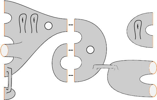
Refer to caption
Figure 2. Two sutured surfaces (right and left) being viewed as morphisms in 2Cobext\Cob^{\ext}; to compose the morphisms one would glue as indicated by the arrows. In the sutured surface language, S+S_{+} is drawn in orange and S−S_{-} is drawn in black, while Λ\Lambda is the set of interface points between the orange and black boundary intervals. Viewing the surfaces as morphisms in 2Cobext\Cob^{\ext}, the source 1-manifold is drawn on the right (ordered from top to bottom) and the target 1-manifold is drawn on the left for each of the two surfaces. To simplify the figure we do not draw orientations.
Remark 2.2.

With the above definition, a sutured surface is the same data as a morphism in the open-closed oriented cobordism category 2Cobext\Cob^{\ext} defined in [LP08]. We view FF as a morphism from M1M_{1} to M2M_{2} where M1M_{1} is given by the orientation reversal of the incoming part of S+S_{+} (a disjoint union, in order, of oriented intervals and circles) and M2M_{2} is given by the outgoing part of S+S_{+}. We take orientations on all parts of the boundary of FF to be induced from the orientation on FF in the usual way without regard to sutured structure. With the boundary orientation we have S+=M2⊔(−M1)S_{+}=M_{2}\sqcup(-M_{1}) where the negative sign denotes orientation reversal.

Remark 2.3.

The reason we need ordering data is to specify unambiguously, for F:M1→M2F\colon M_{1}\to M_{2} a morphism in 2Cobext\Cob^{\ext}, the left action of

A(M1):=ℤ[E]/(E2)⊗⋯⊗ℤ[E]/(E2)A(M_{1}):=\mathbb{Z}[E]/(E^{2})\otimes\cdots\otimes\mathbb{Z}[E]/(E^{2})

and the right action of A⁡(M2)A(M_{2}) on the super abelian group we will associate to FF. We need to know which factor of ℤ⁡[E]/(E2)\mathbb{Z}[E]/(E^{2}) corresponds to which interval.

Figure 2 shows two sutured surfaces being presented as composable morphisms in the category 2Cobext\Cob^{\ext}. Our main gluing theorem, Theorem 1.2, will apply to the type of composition shown in Figure 2, where the 1-manifold along which we are gluing consists only of intervals and no circles.

2.2. Actions on exterior powers

Let (F,Λ,S+,S−,ℓ)(F,\Lambda,S_{+},S_{-},\ell) be a sutured surface. Choose

(A1,A2,A3,A4)∈ℚ4(A_{1},A_{2},A_{3},A_{4})\in\mathbb{Q}^{4}

and let δ:=δA1,A2,A3,A4\delta:=\delta_{A_{1},A_{2},A_{3},A_{4}} as defined in (1). Similarly, choose

(N1,N2,N3,N4)∈{0,1}4(N_{1},N_{2},N_{3},N_{4})\in\{0,1\}^{4}

and let π:=πN1,N2,N3,N4\pi:=\pi_{N_{1},N_{2},N_{3},N_{4}} as defined in (2). Consider the ℤ\mathbb{Z}-graded super abelian group

𝐙δ,πS+(F):=(ℤ0|1)⊗π⁡(F)⊗∧∗H1(F,S+){δ(F)}\mathbf{Z}^{S_{+}}_{\delta,\pi}(F):=\left(\mathbb{Z}^{0|1}\right)^{\otimes\pi(F)}\otimes\wedge^{*}H_{1}(F,S_{+})\{\delta(F)\}

where ℤ0|1\mathbb{Z}^{0|1} denotes ℤ\mathbb{Z} viewed as a purely odd super abelian group. We write εF\varepsilon_{F} for the standard basis element of (ℤ0|1)⊗π⁡(F)\left(\mathbb{Z}^{0|1}\right)^{\otimes\pi(F)}; the parity of εF\varepsilon_{F} is the same as the parity of π⁡(F)\pi(F).

On 𝐙δ,πS+​(F)\mathbf{Z}^{S_{+}}_{\delta,\pi}(F) we will define an action of the superalgebra ℤ⁡[E]/(E2)\mathbb{Z}[E]/(E^{2}) (with EE odd and of degree −1-1) for each interval component II of S+S_{+} by adding signs to the definition over 𝔽2\mathbb{F}_{2} in [Man22]. It suffices to define, given II, a (ℤ\mathbb{Z}-linear) odd endomorphism EE of 𝐙δ,πS+​(F)\mathbf{Z}^{S_{+}}_{\delta,\pi}(F) that has degree −1-1 and squares to zero.

Definition 2.4.

Let (F,Λ,S+,S−,ℓ)(F,\Lambda,S_{+},S_{-},\ell) be a sutured surface and let II be an outgoing interval component of S+S_{+}. We define

E=EI:𝐙δ,πS+​(F)→𝐙δ,πS+​(F)E=E_{I}\colon\mathbf{Z}^{S_{+}}_{\delta,\pi}(F)\to\mathbf{Z}^{S_{+}}_{\delta,\pi}(F)

as follows.

  • •

    Define ϕI:H1​(F,S+)→ℤ\phi_{I}\colon H_{1}(F,S_{+})\to\mathbb{Z} to be the composition

    ϕI:=H1​(F,S+)→∂H0​(S+)→[I]∗⋅−ℤ\phi_{I}:=H_{1}(F,S_{+})\xrightarrow{\partial}H_{0}(S_{+})\xrightarrow{[I]^{*}\cdot-}\mathbb{Z}

    where [I]∗[I]^{*} is the class of H0​(S+)H^{0}(S_{+}) dual to [I]∈H0​(S+)[I]\in H_{0}(S_{+}).

  • •

    For k≥1k\geq 1, define ΦI:Tk​H1​(F,S+)→Tk−1​H1​(F,S+)\Phi_{I}\colon T^{k}H_{1}(F,S_{+})\to T^{k-1}H_{1}(F,S_{+}) by

    (7) ΦI\displaystyle\Phi_{I} :=∑i=1k(Ti−1H1(F,S+)⊗ℤH1(F,S+)⊗ℤTk−iH1(F,S+)\displaystyle:=\sum_{i=1}^{k}\bigg(T^{i-1}H_{1}(F,S_{+})\otimes_{\mathbb{Z}}H_{1}(F,S_{+})\otimes_{\mathbb{Z}}T^{k-i}H_{1}(F,S_{+})
    →(−1)i−1​idTi−1​H1​(F,S+)⊗ϕI⊗idTi−1​H1​(F,S+)Ti−1H1(F,S+)⊗ℤℤ⊗ℤTk−iH1(F,S+).)\displaystyle\xrightarrow{(-1)^{i-1}\id_{T^{i-1}H_{1}(F,S_{+})}\otimes\phi_{I}\otimes\id_{T^{i-1}H_{1}(F,S_{+})}}T^{i-1}H_{1}(F,S_{+})\otimes_{\mathbb{Z}}\mathbb{Z}\otimes_{\mathbb{Z}}T^{k-i}H_{1}(F,S_{+}).\bigg)
  • •

    Because of the sign (−1)i−1(-1)^{i-1} in (7), we get an induced map

    ΦI¯:∧kH1(F,S+)→∧k−1H1(F,S+).\overline{\Phi_{I}}\colon\wedge^{k}H_{1}(F,S_{+})\to\wedge^{k-1}H_{1}(F,S_{+}).

    Define

    ΦI¯′:𝐙δ,πS+​(F)→𝐙δ,πS+​(F)\overline{\Phi_{I}}^{\prime}\colon\mathbf{Z}^{S_{+}}_{\delta,\pi}(F)\to\mathbf{Z}^{S_{+}}_{\delta,\pi}(F)

    by

    ΦI¯′​(εF⊗ω):=(−1)π⁡(F)​εF⊗ΦI¯​(ω).\overline{\Phi_{I}}^{\prime}(\varepsilon_{F}\otimes\omega):=(-1)^{\pi(F)}\varepsilon_{F}\otimes\overline{\Phi_{I}}(\omega).
  • •

    Let EE be the sum of the maps ΦI¯′\overline{\Phi_{I}}^{\prime} over all k≥1k\geq 1. EE is an odd map of degree −1-1 and the sign (−1)i−1(-1)^{i-1} in the definition of ΦI\Phi_{I} ensures that E2=0E^{2}=0.

Define EE similarly when II is an incoming interval component of S+S_{+}, except that:

  • •

    Instead of (−1)i−1(-1)^{i-1} we have (−1)k−i(-1)^{k-i} as the sign in (7);

  • •

    We define

    ΦI¯′:𝐙δ,πS+​(F)→𝐙δ,πS+​(F)\overline{\Phi_{I}}^{\prime}\colon\mathbf{Z}^{S_{+}}_{\delta,\pi}(F)\to\mathbf{Z}^{S_{+}}_{\delta,\pi}(F)

    by

    ΦI¯′​(εF⊗ω):=εF⊗ΦI¯​(ω),\overline{\Phi_{I}}^{\prime}(\varepsilon_{F}\otimes\omega):=\varepsilon_{F}\otimes\overline{\Phi_{I}}(\omega),

    without a sign of (−1)π⁡(F)(-1)^{\pi(F)}.

Remark 2.5.

Because of how we chose the signs above, the actions of ℤ⁡[E]/(E2)\mathbb{Z}[E]/(E^{2}) on 𝐙δ,πS+​(F)\mathbf{Z}^{S_{+}}_{\delta,\pi}(F) for outgoing interval components of S+S_{+} are left actions and the actions for incoming interval components of S+S_{+} are right actions. Correspondingly, we will think of FF as a cobordism “from right to left” in the open-closed cobordism category.

Example 2.6.

For simplicity, choose (N1,N2,N3,N4)(N_{1},N_{2},N_{3},N_{4}) such that for the sutured surface FF shown in Figure 3 (adapted from [Man22, Figure 12]), the parity shift π⁡(F)\pi(F) is even and correspondingly εF\varepsilon_{F} is even. If we let αi\alpha_{i} for 1≤i≤41\leq i\leq 4 denote the arcs and circles shown in Figure 3, then we have

EI​(εF⊗(α1∧α2∧α3∧α4))\displaystyle E_{I}(\varepsilon_{F}\otimes(\alpha_{1}\wedge\alpha_{2}\wedge\alpha_{3}\wedge\alpha_{4})) =εF⊗(−α1∧α2∧α4+α1∧α3∧α4+α1∧α2∧α4)\displaystyle=\varepsilon_{F}\otimes(-\alpha_{1}\wedge\alpha_{2}\wedge\alpha_{4}+\alpha_{1}\wedge\alpha_{3}\wedge\alpha_{4}+\alpha_{1}\wedge\alpha_{2}\wedge\alpha_{4})
=εF⊗(α1∧α3∧α4).\displaystyle=\varepsilon_{F}\otimes(\alpha_{1}\wedge\alpha_{3}\wedge\alpha_{4}).

We could have done the same computation more directly by writing α3\alpha_{3} as a circle rather than an arc with both endpoints on II (in H1​(F,S+)H_{1}(F,S_{+}) there is no difference between these), so that the “remove α3\alpha_{3}” and “remove −α3-\alpha_{3}” terms of EIE_{I} do not appear at all. We drew α3\alpha_{3} as shown in Figure 3 because such arcs often appear in bordered Heegaard Floer homology.

Refer to caption
Figure 3. Examples of oriented arcs and circles in a sutured surface; from this data one can form the element εF⊗(α1∧α2∧α3∧α4)\varepsilon_{F}\otimes(\alpha_{1}\wedge\alpha_{2}\wedge\alpha_{3}\wedge\alpha_{4}) of 𝐙δ,πS+​(F)\mathbf{Z}^{S_{+}}_{\delta,\pi}(F), and Example 2.6 computes EIE_{I} applied to this element. Visually one can think of this application as summing, over all arc endpoints incident with II, of the removal (with appropriate signs, namely ++ for an inward-pointing arc and −- for an outward-pointing arc after doing commutations that move EIE_{I} inward from the left) of the corresponding arc from the wedge product.

The same sign phenomenon responsible for E2=0E^{2}=0 ensures that if II and I′I^{\prime} are two distinct incoming intervals or two distinct outgoing intervals of S+S_{+}, then EIE_{I} and EI′E_{I^{\prime}} anticommute. If II is incoming and I′I^{\prime} is outgoing or vice-versa, then EIE_{I} and EI′E_{I^{\prime}} commute.

If we let minm_{\inn} denote the number of incoming interval components and moutm_{\out} denote the number of outgoing interval components of S+S_{+}, we have A⁡(M1)=(ℤ⁡[E]/(E2))⊗minA(M_{1})=(\mathbb{Z}[E]/(E^{2}))^{\otimes m_{\inn}} and A⁡(M2)=(ℤ⁡[E]/(E2))⊗moutA(M_{2})=(\mathbb{Z}[E]/(E^{2}))^{\otimes m_{\out}}. We thus get the structure of a (left, right) bimodule over the superalgebras (A⁡(M1),A⁡(M2))\left(A(M_{1}),A(M_{2})\right) on 𝐙δ,πS+​(F)\mathbf{Z}^{S_{+}}_{\delta,\pi}(F), where the superalgebra structure on (ℤ⁡[E]/(E2))⊗m(\mathbb{Z}[E]/(E^{2}))^{\otimes m} is the tensor product of superalgebras (so that odd elements in different factors anticommute).

2.3. Tensor products

Here we discuss Example 1.4, about the open pp-tuple of pants 𝒫\mathcal{P}, in more detail. Label the arcs in Figure 4 from top to bottom as e1,…,epe_{1},\ldots,e_{p}. Orient them as shown starting with epe_{p} which points from the outgoing boundary to the incoming boundary; ep−1e_{p-1} should point from the incoming boundary to the outgoing boundary and so forth, in alternating fashion so that e1e_{1} points from outgoing to incoming if pp is odd and from incoming to outgoing if pp is even. See Figure 4. As in Example 1.4, make any choice of (A1,A2,A3,A4)(A_{1},A_{2},A_{3},A_{4}) and (N1,N2,N3,N4)(N_{1},N_{2},N_{3},N_{4}) with A1=1A_{1}=1 and N3=0N_{3}=0. Let δ=δA1,A2,A3,A4\delta=\delta_{A_{1},A_{2},A_{3},A_{4}} and π=πN1,N2,N3,N4\pi=\pi_{N_{1},N_{2},N_{3},N_{4}}.

Refer to caption
Figure 4. Orientations on arcs e1,…,epe_{1},\ldots,e_{p} giving a basis for H1​(𝒫,S+)H_{1}(\mathcal{P},S_{+}).
Proposition 2.7.

Say we are given integers

1≤i1<⋯<ik≤p,1\leq i_{1}<\cdots<i_{k}\leq p,

and we label the elements of {1,…,p}∖{i1,…,ik}\{1,\ldots,p\}\setminus\{i_{1},\ldots,i_{k}\} as

1≤j1<⋯<jp−k≤p.1\leq j_{1}<\cdots<j_{p-k}\leq p.

For 1≤q≤p−k1\leq q\leq p-k let

Ejq:=1⊗⋯1⊗E⊗1⊗⋯⊗1,E_{j_{q}}:=1\otimes\cdots 1\otimes E\otimes 1\otimes\cdots\otimes 1,

an element of (ℤ⁡[E]/(E2))⊗p(\mathbb{Z}[E]/(E^{2}))^{\otimes p}; we can take products of such elements in (ℤ⁡[E]/(E2))⊗p(\mathbb{Z}[E]/(E^{2}))^{\otimes p}. The identification

(8) ε𝒫⊗(ei1∧⋯∧eik)↔Ej1⋯Ejp−k\varepsilon_{\mathcal{P}}\otimes(e_{i_{1}}\wedge\cdots\wedge e_{i_{k}})\quad\leftrightarrow\quad E_{j_{1}}\cdots E_{j_{p-k}}

gives an isomorphism

𝒵δ,πS+​(𝒫)≅(ℤ⁡[E]/(E2))⊗p\mathcal{Z}^{S_{+}}_{\delta,\pi}(\mathcal{P})\cong(\mathbb{Z}[E]/(E^{2}))^{\otimes p}

of ℚ\mathbb{Q}-graded (or ℤ\mathbb{Z}-graded) bimodules over (ℤ⁡[E]/(E2),(ℤ⁡[E]/(E2))⊗p)(\mathbb{Z}[E]/(E^{2}),(\mathbb{Z}[E]/(E^{2}))^{\otimes p}), where the right action of (ℤ⁡[E]/(E2))⊗p(\mathbb{Z}[E]/(E^{2}))^{\otimes p} on (ℤ⁡[E]/(E2))⊗p(\mathbb{Z}[E]/(E^{2}))^{\otimes p} is by multiplication and the left action of ℤ⁡[E]/(E2)\mathbb{Z}[E]/(E^{2}) on (ℤ⁡[E]/(E2))⊗p(\mathbb{Z}[E]/(E^{2}))^{\otimes p} is induced by the coproduct

Δ⁡(E)=E⊗1+1⊗E.\Delta(E)=E\otimes 1+1\otimes E.
Proof.

Example 1.4 ensures that the correspondence (8) respects degrees and parities; because it gives a bijection on basis elements, it is an isomorphism of ℤ\mathbb{Z}-graded super vector spaces. We want to check that (8) respects the left actions of ℤ⁡[E]/(E2)\mathbb{Z}[E]/(E^{2}) and the right actions of (ℤ⁡[E]/(E2))⊗p(\mathbb{Z}[E]/(E^{2}))^{\otimes p}.

First we consider the left action of E∈ℤ⁡[E]/(E2)E\in\mathbb{Z}[E]/(E^{2}). In 𝐙δ,πS+​(𝒫)\mathbf{Z}^{S_{+}}_{\delta,\pi}(\mathcal{P}),

E⋅(ε𝒫⊗(ei1∧⋯∧eik))\displaystyle E\cdot(\varepsilon_{\mathcal{P}}\otimes(e_{i_{1}}\wedge\cdots\wedge e_{i_{k}})) =(−1)π⁡(𝒫)​ε𝒫⊗(E⋅(ei1∧⋯∧eik))\displaystyle=(-1)^{\pi({\mathcal{P}})}\varepsilon_{\mathcal{P}}\otimes(E\cdot(e_{i_{1}}\wedge\cdots\wedge e_{i_{k}}))
=(−1)p​ε𝒫⊗(E⋅(ei1∧⋯∧eik)).\displaystyle=(-1)^{p}\varepsilon_{\mathcal{P}}\otimes(E\cdot(e_{i_{1}}\wedge\cdots\wedge e_{i_{k}})).

The action E⋅(ei1∧⋯∧eik)E\cdot(e_{i_{1}}\wedge\cdots\wedge e_{i_{k}}) is the sum, for 1≤r≤k1\leq r\leq k, of

(−1)r−1​ei1∧⋯∧eir−1∧E⁡(eir)∧eir+1∧⋯∧eik,(-1)^{r-1}e_{i_{1}}\wedge\cdots\wedge e_{i_{r-1}}\wedge E(e_{i_{r}})\wedge e_{i_{r+1}}\wedge\cdots\wedge e_{i_{k}},

and by our choice of orientation on eire_{i_{r}} we have

E⁡(eir)=(−1)p−ir+1⋅1.E(e_{i_{r}})=(-1)^{p-i_{r}+1}\cdot 1.

It follows that E⋅(ε𝒫⊗(ei1∧⋯∧eik))E\cdot(\varepsilon_{\mathcal{P}}\otimes(e_{i_{1}}\wedge\cdots\wedge e_{i_{k}})) is the sum, for 1≤r≤k1\leq r\leq k, of

(−1)ir+r​ei1∧⋯∧eir^∧⋯∧eik,(-1)^{i_{r}+r}e_{i_{1}}\wedge\cdots\wedge\widehat{e_{i_{r}}}\wedge\cdots\wedge e_{i_{k}},

where eir^\widehat{e_{i_{r}}} means we remove the factor eire_{i_{r}} from the wedge product.

Meanwhile, write

Ej1⋯Ejp−k=E⊗⋯⊗E⊗1⊗E⊗⋯⋯⋯⊗E⊗1⊗E⊗⋯⊗E.E_{j_{1}}\cdots E_{j_{p-k}}=E\otimes\cdots\otimes E\otimes 1\otimes E\otimes\cdots\cdots\cdots\otimes E\otimes 1\otimes E\otimes\cdots\otimes E.

When multiplying this expression by EE on the left, the first term will replace the 11 in position i1i_{1} with an EE, picking up a sign of i1−1i_{1}-1. The second term will replace the 11 in position i2i_{2} with an EE, picking up a sign of i2−2i_{2}-2. In general there will be kk terms, and for 1≤r≤k1\leq r\leq k, the rt​hr^{th} term will pick up a sign of ir−ri_{r}-r. Since

(−1)ir+r=(−1)ir−r,(-1)^{i_{r}+r}=(-1)^{i_{r}-r},

the identification (8) is compatible with the left actions of ℤ⁡[E]/(E2)\mathbb{Z}[E]/(E^{2}).

Now consider the right action of EE in the mt​hm^{th} factor of (ℤ⁡[E]/(E2))⊗p(\mathbb{Z}[E]/(E^{2}))^{\otimes p}, for 1≤m≤p1\leq m\leq p; call this element EmE_{m}. We have

(ε𝒫⊗(ei1∧⋯∧eik))⋅Em=0(\varepsilon_{\mathcal{P}}\otimes(e_{i_{1}}\wedge\cdots\wedge e_{i_{k}}))\cdot E_{m}=0

unless m=irm=i_{r} for some rr, and we have

(ε𝒫⊗(ei1∧⋯∧eik))⋅Eir\displaystyle(\varepsilon_{\mathcal{P}}\otimes(e_{i_{1}}\wedge\cdots\wedge e_{i_{k}}))\cdot E_{i_{r}}
=(−1)k−r​ε𝒫⊗(ei1∧⋯∧eir−1∧(eir⋅E)∧eir+1∧⋯∧eik).\displaystyle=(-1)^{k-r}\varepsilon_{\mathcal{P}}\otimes(e_{i_{1}}\wedge\cdots\wedge e_{i_{r-1}}\wedge(e_{i_{r}}\cdot E)\wedge e_{i_{r+1}}\wedge\cdots\wedge e_{i_{k}}).

By our choice of orientation on eire_{i_{r}}, we have eir⋅E=(−1)p−ir⋅1e_{i_{r}}\cdot E=(-1)^{p-i_{r}}\cdot 1, so (εF⊗(ei1∧⋯∧eik))⋅Eir(\varepsilon_{F}\otimes(e_{i_{1}}\wedge\cdots\wedge e_{i_{k}}))\cdot E_{i_{r}} equals

(−1)p+k−ir−r​ε𝒫⊗(ei1∧⋯∧eir^∧⋯∧eik).(-1)^{p+k-i_{r}-r}\varepsilon_{\mathcal{P}}\otimes(e_{i_{1}}\wedge\cdots\wedge\widehat{e_{i_{r}}}\wedge\cdots\wedge e_{i_{k}}).

Meanwhile, writing Ej1⋯Ejn−kE_{j_{1}}\cdots E_{j_{n-k}} as a tensor product of 11s and EEs as above, we see that (Ej1⋯Ejn−k)⋅Em(E_{j_{1}}\cdots E_{j_{n-k}})\cdot E_{m} is also zero unless m=irm=i_{r} for some rr.

  • •

    For r=kr=k, when computing (Ej1⋯Ejn−k)⋅Eik(E_{j_{1}}\cdots E_{j_{n-k}})\cdot E_{i_{k}}, to reach the 11 that will be replaced by EE, the odd element EikE_{i_{k}} will need to commute past p−ikp-i_{k} instances of EE, picking up a sign of (−1)p−ik(-1)^{p-i_{k}}.

  • •

    For r=k−1r=k-1, when computing (Ej1⋯Ejn−k)⋅Eik−1(E_{j_{1}}\cdots E_{j_{n-k}})\cdot E_{i_{k-1}}, the odd element Eik−1E_{i_{k-1}} will need to commute past p−ik−1−1p-i_{k-1}-1 instances of EE, picking up a sign of (−1)k−ik−1−1(-1)^{k-i_{k-1}-1}.

In general, when computing (Ej1⋯Ejn−k)⋅Eik−q(E_{j_{1}}\cdots E_{j_{n-k}})\cdot E_{i_{k-q}}, the odd element Eik−qE_{i_{k-q}} will need to commute past p−ik−q−qp-i_{k-q}-q instances of EE, picking up a sign of (−1)p−ik−q−q(-1)^{p-i_{k-q}-q}. Reindexing k−qk-q as rr, we see that the sign in front of (Ej1⋯Ejn−k)⋅Eir(E_{j_{1}}\cdots E_{j_{n-k}})\cdot E_{i_{r}} is (−1)p−ir−(k−r)(-1)^{p-i_{r}-(k-r)}, which equals (−1)p+k−ir−r(-1)^{p+k-i_{r}-r} as desired. ∎

As mentioned in Example 1.4, the correspondence (8) identifies the highest-degree element of 𝐙δ,πS+​(𝒫)\mathbf{Z}^{S_{+}}_{\delta,\pi}(\mathcal{P}) (defined up to a sign) with ±1∈(ℤ⁡[E]/(E2))⊗p\pm 1\in(\mathbb{Z}[E]/(E^{2}))^{\otimes p}.

3. A gluing theorem with signs and gradings

3.1. The main gluing lemma

The following is a version with signs and gradings of the main gluing lemma from [Man22]. Let (F,Λ,S+,S−,ℓ)(F,\Lambda,S_{+},S_{-},\ell) be a sutured surface with all S+S_{+} boundary components considered to be outgoing, and suppose that I1,I2I_{1},I_{2} are interval components of S+S_{+}. As in [Man22], there is a unique way up to homeomorphism to glue I1I_{1} to I2I_{2} and get an oriented surface F¯\overline{F}, which can itself be viewed as a sutured surface with all S+S_{+} boundary components outgoing (we will let S+S_{+} denote the S+S_{+} boundary of either FF or F¯\overline{F}, determined by context). Let δ=δA1,A2,A3,A4\delta=\delta_{A_{1},A_{2},A_{3},A_{4}} and π=πN1,N2,N3,N4\pi=\pi_{N_{1},N_{2},N_{3},N_{4}} for any (A1,A2,A3,A4)∈ℚ4(A_{1},A_{2},A_{3},A_{4})\in\mathbb{Q}^{4} and (N1,N2,N3,N4)∈{0,1}4(N_{1},N_{2},N_{3},N_{4})\in\{0,1\}^{4}. Let E1E_{1} and E2E_{2} denote the EE-endomorphisms of 𝐙δ,πS+​(F)\mathbf{Z}^{S_{+}}_{\delta,\pi}(F) arising from I1I_{1} and I2I_{2} respectively.

Lemma 3.1 (cf. Lemma 4.1 of [Man22]).

We have an isomorphism

𝐙δ,πS+​(F¯)≅𝐙δ,πS+​(F)im⁡(E1+E2)\mathbf{Z}^{S_{+}}_{\delta,\pi}(\overline{F})\cong\frac{\mathbf{Z}^{S_{+}}_{\delta,\pi}(F)}{\im(E_{1}+E_{2})}

of ℚ\mathbb{Q}-graded super abelian groups, compatible with the left actions of ℤ⁡[E]/(E2)\mathbb{Z}[E]/(E^{2}) coming from S+S_{+} intervals of FF that are not in {I1,I2}\{I_{1},I_{2}\}.

Before proving Lemma 3.1 we will discuss a way of choosing bases for ∧∗H1(F,S+)\wedge^{*}H_{1}(F,S_{+}) following [Man22, proof of Lemma 4.1].

Definition 3.2.

For a sutured surface FF, choose a homeomorphism between FF and a finite disjoint union of “standard” sutured surfaces (Figure 5), each consisting of a sphere connect-summed with some number of tori and with some number of open disks removed, with an even number of sutures on each boundary component. Then define a collection of arcs and circles in each standard sutured surface as follows.

  • •

    In each torus that was connect-summed on, take two circles giving a basis for the first homology.

  • •

    For all of the boundary components intersecting S−S_{-} nontrivially, except for one chosen component, take a circle around the boundary component.

  • •

    Take a connected acyclic graph ΓF\Gamma_{F} embedded in FF with vertices in S+S_{+} (one vertex in each component of S+S_{+}).

  • •

    Since we are working over ℤ\mathbb{Z}, we also need to choose orientations on the arcs and circles used to define this basis.

See Figure 6 for an illustration. The circles and the edges of ΓF\Gamma_{F} give a basis for H1​(F,S+)H_{1}(F,S_{+}), so subsets (corresponding to wedge products) of the set of arcs and circles give a basis for ∧∗H1(F,S+)\wedge^{*}H_{1}(F,S_{+}). The same construction gives a basis for 𝐙δ,πS+​(F)\mathbf{Z}^{S_{+}}_{\delta,\pi}(F). We will refer to the circles and the edges of ΓF\Gamma_{F} as basis arcs and basis circles.

Remark 3.3.

If we always have in mind the bases of Definition 3.2, which will be the case below, then the quantity h=rank⁡H1​(F,S+)h=\rk H_{1}(F,S_{+}) is the number of basis arcs and circles. When self-gluing FF to get a new surface F¯\overline{F} below, to see how hh changes one can simply compare the number of basis arcs and circles before and after the self-gluing. Combinatorially, we have

(9) h=\displaystyle h= −2​#​{components of ​F}+2​#​{genus}\displaystyle-2\#\{\textrm{components of }F\}+2\#\{\textrm{genus}\}
+#⁡{no-​S+​ non-closed components of ​F}\displaystyle+\#\{\textrm{no-}S_{+}\textrm{ non-closed components of }F\}
+#⁡{no-​S−​ non-closed components of ​F}\displaystyle+\#\{\textrm{no-}S_{-}\textrm{ non-closed components of }F\}
+2​#​{closed components of ​F}\displaystyle+2\#\{\textrm{closed components of }F\}
+#⁡{S+​ intervals}+#⁡{S+​ circles}\displaystyle+\#\{S_{+}\textrm{ intervals}\}+\#\{S_{+}\textrm{ circles}\}
+#⁡{S−​ circles}+#⁡{boundary circles of ​F​ with both ​S+​ and ​S−}\displaystyle+\#\{S_{-}\textrm{ circles}\}+\#\{\textrm{boundary circles of }F\textrm{ with both }S_{+}\textrm{ and }S_{-}\}

where by the genus of FF we mean the sum of the genus of each component of FF.

Refer to caption
Figure 5. A standard (connected) sutured surface; on the boundary, S+S_{+} is drawn in orange and S−S_{-} is drawn in black. The sutures are the interface points between orange and black regions of the boundary.
Refer to caption
Figure 6. Examples of oriented arcs and circles used to specify a basis for ∧∗H1(F,S+)\wedge^{*}H_{1}(F,S_{+}).
Proof of Lemma 3.1.

We will break the proof into cases.

Case 1: I1I_{1} and I2I_{2} are on distinct components of FF. Assume that I1I_{1} and I2I_{2} live on distinct connected components of FF. Begin by choosing a ℤ\mathbb{Z}-basis for ∧∗H1(F,S+)\wedge^{*}H_{1}(F,S_{+}) as in Definition 3.2; without loss of generality we may assume that I1I_{1} and I2I_{2} are each incident with at most one basis arc.

Case 1-1: I1I_{1} and I2I_{2} are both alone. Suppose that the components of FF containing I1I_{1} and I2I_{2} each contain no other components of S+S_{+}. In this case, no basis arcs are incident with either I1I_{1} or I2I_{2}. We have δ⁡(F)=δ⁡(F¯)\delta(F)=\delta(\overline{F}), π⁡(F)=π⁡(F¯)\pi(F)=\pi(\overline{F}), and H1​(F,S+)≅H1​(F¯,S+)H_{1}(F,S_{+})\cong H_{1}(\overline{F},S_{+}). Both E1E_{1} and E2E_{2} act as zero on 𝐙δ,πS+​(F)\mathbf{Z}^{S_{+}}_{\delta,\pi}(F), implying the statement of the lemma.

Case 1-2: only I2I_{2} is alone. Now suppose exactly one of {I1,I2}\{I_{1},I_{2}\} (without loss of generality I2I_{2}) is the unique component of S+S_{+} in its component of FF. In this case, I1I_{1} is incident with one basis arc e1e_{1}, while I2I_{2} is not incident with any basis arc. Without loss of generality, assume e1e_{1} points from the surface into I1I_{1}.

The endomorphism E2E_{2} of 𝐙δ,πS+​(F)\mathbf{Z}^{S_{+}}_{\delta,\pi}(F) is zero. Let ω\omega be a basis element for ∧∗H1(F,S+)\wedge^{*}H_{1}(F,S_{+}); the action of E1E_{1} on εF⊗ω\varepsilon_{F}\otimes\omega is zero unless e1e_{1} is the it​hi^{th} wedge factor of ω\omega for some ii, in which case write

ω=γ1∧⋯∧γi−1∧e1∧γi+1∧⋯∧γk\omega=\gamma_{1}\wedge\cdots\wedge\gamma_{i-1}\wedge e_{1}\wedge\gamma_{i+1}\wedge\cdots\wedge\gamma_{k}

where the γj\gamma_{j} are basis elements for H1​(F,S+)H_{1}(F,S_{+}). If we set

ω′=γ1∧⋯∧γi−1∧γi+1∧⋯∧γk,\omega^{\prime}=\gamma_{1}\wedge\cdots\wedge\gamma_{i-1}\wedge\gamma_{i+1}\wedge\cdots\wedge\gamma_{k},

then E1​(εF⊗ω)=(−1)π⁡(F)+i−1​εF⊗ω′E_{1}(\varepsilon_{F}\otimes\omega)=(-1)^{\pi(F)+i-1}\varepsilon_{F}\otimes\omega^{\prime}. We see that the quotient in the statement of the lemma amounts to setting εF⊗ω′\varepsilon_{F}\otimes\omega^{\prime} equal to zero whenever ω′\omega^{\prime} is a basis element of ∧∗H1(F,S+)\wedge^{*}H_{1}(F,S_{+}) not divisible by e1e_{1}. Thus, we can take the elements

εF⊗(e1∧ω′),\varepsilon_{F}\otimes\left(e_{1}\wedge\omega^{\prime}\right),

where ω′\omega^{\prime} is not divisible by e1e_{1}, as a ℤ\mathbb{Z}-basis for the quotient.

Now if we take all the basis arcs and circles, and remove e1e_{1}, the remaining arcs and circles can be used to define a basis of H1​(F¯,S+)H_{1}(\overline{F},S_{+}). The corresponding ℤ\mathbb{Z}-basis for 𝐙δ,πS+​(F¯)\mathbf{Z}^{S_{+}}_{\delta,\pi}(\overline{F}) is given by the set of elements εF¯⊗ω′\varepsilon_{\overline{F}}\otimes\omega^{\prime} where ω′\omega^{\prime} is as above. The identification

(10) εF⊗(e1∧ω′)↔εF¯⊗ω′\varepsilon_{F}\otimes\left(e_{1}\wedge\omega^{\prime}\right)\quad\leftrightarrow\quad\varepsilon_{\overline{F}}\otimes\omega^{\prime}

gives a map from the quotient to OPEN𝐙δ,πS+​(F¯))\mathbf{Z}^{S_{+}}_{\delta,\pi}(\overline{F})).

When passing from FF to F¯\overline{F}, the changes in quantities relevant for the definitions of δ\delta and π\pi are as follows.

  • •

    hh is decreased by 11.

  • •

    The number of S+S_{+} intervals is decreased by 22.

The change in δ\delta is thus A1−(A1−1)=+1A_{1}-(A_{1}-1)=+1, and the change in π\pi is −1−2​N3=1-1-2N_{3}=1 modulo 22. Thus, (10) is an even map of degree zero; it is an isomorphism of super abelian groups because it gives a bijection on basis elements.

To see that this isomorphism intertwines the remaining actions, let I∉{I1,I2}I\notin\{I_{1},I_{2}\} be an interval component of S+S_{+}. First assume e1e_{1} is not incident with II. In this case, the endomorphism EIE_{I} of 𝐙δ,πS+​(F)im⁡(E1+E2)\frac{\mathbf{Z}^{S_{+}}_{\delta,\pi}(F)}{\im(E_{1}+E_{2})} corresponding to II sends a basis element εF⊗(e1∧ω′)\varepsilon_{F}\otimes(e_{1}\wedge\omega^{\prime}) to (−1)π⁡(F)+1​εF⊗(e1∧EI​(ω′))(-1)^{\pi(F)+1}\varepsilon_{F}\otimes\left(e_{1}\wedge E_{I}(\omega^{\prime})\right). Meanwhile, the endomorphism EIE_{I} of 𝐙δ,πS+​(F¯)\mathbf{Z}^{S_{+}}_{\delta,\pi}(\overline{F}) sends εF¯⊗ω′\varepsilon_{\overline{F}}\otimes\omega^{\prime} to (−1)π⁡(F¯)​εF¯⊗EI​(ω′)(-1)^{\pi(\overline{F})}\varepsilon_{\overline{F}}\otimes E_{I}(\omega^{\prime}). Our identification sends

(−1)π⁡(F)+1εF⊗(e1∧EI(ω′))↔(−1)π⁡(F¯)εF¯⊗EI(ω′)(-1)^{\pi(F)+1}\varepsilon_{F}\otimes\left(e_{1}\wedge E_{I}(\omega^{\prime})\right)\quad\leftrightarrow\quad(-1)^{\pi(\overline{F})}\varepsilon_{\overline{F}}\otimes E_{I}(\omega^{\prime})

because π⁡(F¯)=π⁡(F)−1\pi(\overline{F})=\pi(F)-1. If e1e_{1} is incident with II, the analysis is unchanged because the extra term we would get in 𝐙δ,πS+​(F)\mathbf{Z}^{S_{+}}_{\delta,\pi}(F) vanishes in the quotient

𝐙δ,πS+​(F)im⁡(E1+E2)=𝐙δ,πS+​(F)im⁡(E1).\frac{\mathbf{Z}^{S_{+}}_{\delta,\pi}(F)}{\im(E_{1}+E_{2})}=\frac{\mathbf{Z}^{S_{+}}_{\delta,\pi}(F)}{\im(E_{1})}.

Case 1-3: neither I1I_{1} nor I2I_{2} is alone. Now we consider the generic case; for j∈{1,2}j\in\{1,2\}, IjI_{j} is incident with a unique arc eje_{j} used to define the basis of H1​(F,S+)H_{1}(F,S_{+}). Orient e1e_{1} so that it points from the surface into I1I_{1}, and orient e2e_{2} so that it points from I2I_{2} into the surface. Choose the other orientations arbitrarily.

As a left module over (ℤ⁡[E]/(E2))⊗2(\mathbb{Z}[E]/(E^{2}))^{\otimes 2} (with jt​hj^{th} factor corresponding to EjE_{j} for j∈{1,2}j\in\{1,2\}), 𝐙δ,πS+​(F)\mathbf{Z}^{S_{+}}_{\delta,\pi}(F) is free with a basis given by the set of elements

εF⊗(e1∧e2∧ω′),\varepsilon_{F}\otimes(e_{1}\wedge e_{2}\wedge\omega^{\prime}),

where ω′\omega^{\prime} is a ℤ\mathbb{Z}-basis element for ∧∗H1(F,S+)\wedge^{*}H_{1}(F,S_{+}) with neither e1e_{1} nor e2e_{2} as factors. Applying E1E_{1} (which “removes e1e_{1}”) to εF⊗(e1∧e2∧ω′)\varepsilon_{F}\otimes(e_{1}\wedge e_{2}\wedge\omega^{\prime}) gives

(−1)π⁡(F)​εF⊗(e2∧ω′),(-1)^{\pi(F)}\varepsilon_{F}\otimes(e_{2}\wedge\omega^{\prime}),

applying E1E_{1} to εF⊗(e1∧ω′)\varepsilon_{F}\otimes(e_{1}\wedge\omega^{\prime}) gives

(−1)π⁡(F)​εF⊗ω′,(-1)^{\pi(F)}\varepsilon_{F}\otimes\omega^{\prime},

and applying E1E_{1} to εF⊗(e2∧ω′)\varepsilon_{F}\otimes(e_{2}\wedge\omega^{\prime}) or εF⊗ω′\varepsilon_{F}\otimes\omega^{\prime} gives zero. Similarly, applying E2E_{2} (which “removes −e2-e_{2}”) to εF⊗(e1∧e2∧ω′)\varepsilon_{F}\otimes(e_{1}\wedge e_{2}\wedge\omega^{\prime}) gives

(−1)π⁡(F)​εF⊗(e1∧ω′),(-1)^{\pi(F)}\varepsilon_{F}\otimes(e_{1}\wedge\omega^{\prime}),

applying E2E_{2} to εF⊗(e2∧ω′)\varepsilon_{F}\otimes(e_{2}\wedge\omega^{\prime}) gives

(−1)π⁡(F)+1​εF⊗ω′,(-1)^{\pi(F)+1}\varepsilon_{F}\otimes\omega^{\prime},

and applying E2E_{2} to εF⊗(e1∧ω′)\varepsilon_{F}\otimes(e_{1}\wedge\omega^{\prime}) or εF⊗ω′\varepsilon_{F}\otimes\omega^{\prime} gives zero.

It follows that a ℤ\mathbb{Z}-basis for 𝐙δ,πS+​(F)im⁡(E1+E2)\frac{\mathbf{Z}^{S_{+}}_{\delta,\pi}(F)}{\im(E_{1}+E_{2})} can be specified by taking the elements εF⊗(e1∧e2∧ω′)\varepsilon_{F}\otimes(e_{1}\wedge e_{2}\wedge\omega^{\prime}) along with the elements

εF⊗(e1∧ω′)=−εF⊗(e2∧ω′).\varepsilon_{F}\otimes(e_{1}\wedge\omega^{\prime})=-\varepsilon_{F}\otimes(e_{2}\wedge\omega^{\prime}).

Now, if we let ee be the oriented arc in F¯\overline{F} obtained by concatenating e1e_{1} and e2e_{2}, then a ℤ\mathbb{Z}-basis for 𝐙δ,πS+​(F¯)\mathbf{Z}^{S_{+}}_{\delta,\pi}(\overline{F}) is given by the set of elements εF¯⊗(e∧ω′)\varepsilon_{\overline{F}}\otimes(e\wedge\omega^{\prime}) and εF¯⊗ω′\varepsilon_{\overline{F}}\otimes\omega^{\prime} where ω′\omega^{\prime} runs over the same set as above. Make the identifications

εF⊗(e1∧e2∧ω′)↔εF¯⊗(e∧ω′)\varepsilon_{F}\otimes(e_{1}\wedge e_{2}\wedge\omega^{\prime})\quad\leftrightarrow\quad\varepsilon_{\overline{F}}\otimes(e\wedge\omega^{\prime})

and

εF⊗(e1∧ω′)↔εF¯⊗ω′;\varepsilon_{F}\otimes(e_{1}\wedge\omega^{\prime})\quad\leftrightarrow\quad\varepsilon_{\overline{F}}\otimes\omega^{\prime};

this is an even map of degree zero because π⁡(F¯)=π⁡(F)+1\pi(\overline{F})=\pi(F)+1 (the same argument applies as in the previous case). We get an isomorphism of ℤ\mathbb{Z}-graded super abelian groups as claimed in the statement of the lemma.

To see that this isomorphism intertwines the remaining actions, let I∉{I1,I2}I\notin\{I_{1},I_{2}\} be an interval component of S+S_{+}.

Case 1-3a: II is disjoint from {e1,e2}\{e_{1},e_{2}\}. First assume that neither e1e_{1} nor e2e_{2} is incident with II. In this case, the endomorphism EIE_{I} of 𝐙δ,πS+​(F)im⁡(E1+E2)\frac{\mathbf{Z}^{S_{+}}_{\delta,\pi}(F)}{\im(E_{1}+E_{2})} corresponding to II sends a basis element εF⊗(e1∧e2∧ω′)\varepsilon_{F}\otimes(e_{1}\wedge e_{2}\wedge\omega^{\prime}) to

(−1)π⁡(F)​εF⊗(e1∧e2∧EI​(ω′)).(-1)^{\pi(F)}\varepsilon_{F}\otimes\left(e_{1}\wedge e_{2}\wedge E_{I}(\omega^{\prime})\right).

It sends a basis element εF⊗(e1∧ω′)\varepsilon_{F}\otimes(e_{1}\wedge\omega^{\prime}) to

(−1)π⁡(F)+1​εF⊗(e1∧EI​(ω′)).(-1)^{\pi(F)+1}\varepsilon_{F}\otimes(e_{1}\wedge E_{I}(\omega^{\prime})).

Meanwhile, the endomorphism EIE_{I} of OPEN𝐙δ,πS+​(F¯))\mathbf{Z}^{S_{+}}_{\delta,\pi}(\overline{F})) sends εF¯⊗(e∧ω′)\varepsilon_{\overline{F}}\otimes(e\wedge\omega^{\prime}) to

(−1)π⁡(F¯)+1​εF¯⊗(e∧EI​(ω′))=(−1)π⁡(F)​εF¯⊗(e∧EI​(ω′))(-1)^{\pi(\overline{F})+1}\varepsilon_{\overline{F}}\otimes(e\wedge E_{I}(\omega^{\prime}))=(-1)^{\pi(F)}\varepsilon_{\overline{F}}\otimes(e\wedge E_{I}(\omega^{\prime}))

and it sends εF¯⊗ω′\varepsilon_{\overline{F}}\otimes\omega^{\prime} to

(−1)π⁡(F¯)​εF¯⊗EI​(ω′)=(−1)π⁡(F)+1​εF¯⊗EI​(ω′).(-1)^{\pi(\overline{F})}\varepsilon_{\overline{F}}\otimes E_{I}(\omega^{\prime})=(-1)^{\pi(F)+1}\varepsilon_{\overline{F}}\otimes E_{I}(\omega^{\prime}).

Our identification sends

(−1)π⁡(F)εF⊗(e1∧e2∧EI(ω′))↔(−1)π⁡(F)εF¯⊗(e∧EI(ω′))(-1)^{\pi(F)}\varepsilon_{F}\otimes\left(e_{1}\wedge e_{2}\wedge E_{I}(\omega^{\prime})\right)\quad\leftrightarrow\quad(-1)^{\pi(F)}\varepsilon_{\overline{F}}\otimes(e\wedge E_{I}(\omega^{\prime}))

and

(−1)π⁡(F)+1​εF⊗(e1∧EI​(ω′))↔(−1)π⁡(F)+1​εF¯⊗EI​(ω′),(-1)^{\pi(F)+1}\varepsilon_{F}\otimes(e_{1}\wedge E_{I}(\omega^{\prime}))\leftrightarrow(-1)^{\pi(F)+1}\varepsilon_{\overline{F}}\otimes E_{I}(\omega^{\prime}),

so it intertwines the actions of EIE_{I} on the two sides.

Case 1-3b: II is incident with e1e_{1}. Now suppose II is incident with e1e_{1}; because e1e_{1} points from the surface into I1I_{1}, it must point from II into the surface. The same is true for ee in F¯\overline{F}.

Some terms of the action on EIE_{I} on each side (where neither e1e_{1} nor ee is removed) are similar to the ones in Case 1-3a and thus correspond to each other under our identification. We also have a new term of EI​(εF⊗(e1∧e2∧ω′))E_{I}(\varepsilon_{F}\otimes(e_{1}\wedge e_{2}\wedge\omega^{\prime})), namely the “remove (−e1)(-e_{1})” term

(−1)π⁡(F)+1​εF⊗(e2∧ω′)=(−1)π⁡(F)​εF⊗(e1∧ω′),(-1)^{\pi(F)+1}\varepsilon_{F}\otimes(e_{2}\wedge\omega^{\prime})=(-1)^{\pi(F)}\varepsilon_{F}\otimes(e_{1}\wedge\omega^{\prime}),

and a new term of EI​(εF¯⊗(e∧ω′))E_{I}(\varepsilon_{\overline{F}}\otimes(e\wedge\omega^{\prime})), namely the “remove (−e)(-e)” term

(−1)π⁡(F¯)+1​εF⊗ω′=(−1)π⁡(F)​εF⊗ω′.(-1)^{\pi(\overline{F})+1}\varepsilon_{F}\otimes\omega^{\prime}=(-1)^{\pi(F)}\varepsilon_{F}\otimes\omega^{\prime}.

These terms correspond to each other under our identification.

Case 1-3c: II is incident with e2e_{2}.

In this case e2e_{2} and ee point from the surface into II, so the new terms are the “remove e2e_{2}” term of EI​(εF⊗(e1∧e2∧ω′))E_{I}(\varepsilon_{F}\otimes(e_{1}\wedge e_{2}\wedge\omega^{\prime})), namely

(−1)π⁡(F)+1​εF⊗(e1∧ω′),(-1)^{\pi(F)+1}\varepsilon_{F}\otimes(e_{1}\wedge\omega^{\prime}),

and the “remove ee” term of EI​(εF¯⊗(e∧ω′))E_{I}(\varepsilon_{\overline{F}}\otimes(e\wedge\omega^{\prime})), namely

(−1)π⁡(F¯)​εF¯⊗ω′=(−1)π⁡(F)+1​εF¯⊗ω′.(-1)^{\pi(\overline{F})}\varepsilon_{\overline{F}}\otimes\omega^{\prime}=(-1)^{\pi(F)+1}\varepsilon_{\overline{F}}\otimes\omega^{\prime}.

These terms correspond to each other under our identification.

Case 2: I1I_{1} and I2I_{2} are on the same component of FF. We consider some further subcases.

Case 2-1: I1I_{1} and I2I_{2} are on the same component of ∂F\partial F. Let γ\gamma be the component of ∂F\partial F containing I1I_{1} and I2I_{2}. When applying Definition 3.2 to choose a basis for H1​(F,S+)H_{1}(F,S_{+}), choose γ\gamma as the unique not-fully-S+S_{+} boundary component of its component of FF that does not get a basis circle around it, and such that I1I_{1} and I2I_{2} are incident with a single basis arc each, say e1e_{1} and e2e_{2} respectively (it is possible that e1=e2e_{1}=e_{2}). Orient e1e_{1} so it points from the surface into I1I_{1} and orient e2e_{2} so it points from I2I_{2} into the surface; this makes sense even if e1=e2e_{1}=e_{2}.

Refer to caption
Figure 7. Local model near the circle CC for the arcs e1e_{1} and e2e_{2} and the circle σ\sigma in Case 2-1a.

Case 2-1a: I1I_{1} and I2I_{2} are not alone in their component of FF. Assume the component of FF containing I1I_{1} and I2I_{2} also contains at least one other S+S_{+} interval or S+S_{+} circle. In this case we can assume that e1≠e2e_{1}\neq e_{2}, and we can also assume that e1e_{1} and e2e_{2} share an endpoint qq, as in [Man22, Figure 19] or the analogue of that figure when qq is on the same component of ∂F\partial F as I1I_{1} and I2I_{2}. See Figure 7 here for illustrations of both possibilities.

With respect to e1e_{1} and e2e_{2}, there are four types of ℤ\mathbb{Z}-basis elements for 𝐙δ,πS+​(F)\mathbf{Z}^{S_{+}}_{\delta,\pi}(F), namely those of type εF⊗(e1∧e2∧ω′)\varepsilon_{F}\otimes(e_{1}\wedge e_{2}\wedge\omega^{\prime}), εF⊗(e1∧ω′)\varepsilon_{F}\otimes(e_{1}\wedge\omega^{\prime}), εF⊗(e2∧ω′)\varepsilon_{F}\otimes(e_{2}\wedge\omega^{\prime}), and εF⊗ω′\varepsilon_{F}\otimes\omega^{\prime} where ω′\omega^{\prime} is not divisible by e1e_{1} or e2e_{2}. We have

E1​(εF⊗(e1∧e2∧ω′))=(−1)π⁡(F)​εF⊗(e2∧ω′)E_{1}(\varepsilon_{F}\otimes(e_{1}\wedge e_{2}\wedge\omega^{\prime}))=(-1)^{\pi(F)}\varepsilon_{F}\otimes(e_{2}\wedge\omega^{\prime})

because E1E_{1} removes e1e_{1} from the left, and

E2​(εF⊗(e1∧e2∧ω′))=(−1)π⁡(F)​εF⊗(e1∧ω′)E_{2}(\varepsilon_{F}\otimes(e_{1}\wedge e_{2}\wedge\omega^{\prime}))=(-1)^{\pi(F)}\varepsilon_{F}\otimes(e_{1}\wedge\omega^{\prime})

because E2E_{2} removes (−e2)(-e_{2}) from the left. Thus, in the quotient 𝐙δ,πS+​(F)im⁡(E1+E2)\frac{\mathbf{Z}^{S_{+}}_{\delta,\pi}(F)}{\im(E_{1}+E_{2})}, we have

εF⊗(e2∧ω′)=−εF⊗(e1∧ω′)\varepsilon_{F}\otimes(e_{2}\wedge\omega^{\prime})=-\varepsilon_{F}\otimes(e_{1}\wedge\omega^{\prime})

as well as

εF⊗ω′=0.\varepsilon_{F}\otimes\omega^{\prime}=0.

Meanwhile, to define ΓF¯\Gamma_{\overline{F}}, remove e1e_{1} and e2e_{2} as basis arcs and add a basis circle σ\sigma oriented compatibly with e1e_{1} and e2e_{2} (see Figure 7). There are two types of basis elements of 𝐙δ,πS+​(F¯)\mathbf{Z}^{S_{+}}_{\delta,\pi}(\overline{F}), namely those of type εF⊗(σ∧ω′)\varepsilon_{F}\otimes(\sigma\wedge\omega^{\prime}) and εF⊗ω′\varepsilon_{F}\otimes\omega^{\prime} where ω′\omega^{\prime} is not divisible by σ\sigma. Make the identifications

(11) εF⊗(e1∧e2∧ω′)↔εF¯⊗(σ∧ω′)\varepsilon_{F}\otimes(e_{1}\wedge e_{2}\wedge\omega^{\prime})\quad\leftrightarrow\quad\varepsilon_{\overline{F}}\otimes(\sigma\wedge\omega^{\prime})

and

(12) εF⊗(e1∧ω′)↔εF¯⊗ω′.\varepsilon_{F}\otimes(e_{1}\wedge\omega^{\prime})\quad\leftrightarrow\quad\varepsilon_{\overline{F}}\otimes\omega^{\prime}.

When passing from FF to F¯\overline{F}, the changes in quantities relevant for the definitions of δ\delta and π\pi are the same as the ones described above. The change in δ\delta is thus A1−(A1−1)=+1A_{1}-(A_{1}-1)=+1, and the change in π\pi is −1−2​N3=1-1-2N_{3}=1 modulo 22. Because π⁡(F¯)=π⁡(F)+1\pi(\overline{F})=\pi(F)+1, the identifications (11) and (12) give an even map of degree zero and thus an isomorphism of ℤ\mathbb{Z}-graded super abelian groups. The relation π⁡(F¯)=π⁡(F)+1\pi(\overline{F})=\pi(F)+1 also ensures that this identification intertwines the actions of EI′E_{I^{\prime}} for any S+S_{+} interval component I′I^{\prime} not in {I1,I2}\{I_{1},I_{2}\}, except possibly the interval II containing qq (if qq is contained in an S+S_{+} interval rather than an S+S_{+} circle). If qq is contained in an S+S_{+} interval II, we have

EI​(εF⊗(e1∧e2∧ω′))\displaystyle E_{I}(\varepsilon_{F}\otimes(e_{1}\wedge e_{2}\wedge\omega^{\prime}))
=(−1)π⁡(F)​εF⊗(e2∧ω′)+(−1)h​π​(F)+2​εF⊗(e1∧ω′)+(−1)π⁡(F)+2​εF⊗(e1∧e2∧EI​(ω′))\displaystyle=(-1)^{\pi(F)}\varepsilon_{F}\otimes(e_{2}\wedge\omega^{\prime})+(-1)^{h\pi(F)+2}\varepsilon_{F}\otimes(e_{1}\wedge\omega^{\prime})+(-1)^{\pi(F)+2}\varepsilon_{F}\otimes(e_{1}\wedge e_{2}\wedge E_{I}(\omega^{\prime}))
=(−1)π⁡(F)(−εF⊗(e1∧ω′)+εF⊗(e1∧ω′)+εF⊗(e1∧e2∧EI(ω′)))\displaystyle=(-1)^{\pi(F)}\left(-\varepsilon_{F}\otimes(e_{1}\wedge\omega^{\prime})+\varepsilon_{F}\otimes(e_{1}\wedge\omega^{\prime})+\varepsilon_{F}\otimes(e_{1}\wedge e_{2}\wedge E_{I}(\omega^{\prime}))\right)
=(−1)π⁡(F)​εF⊗(e1∧e2∧EI​(ω′))\displaystyle=(-1)^{\pi(F)}\varepsilon_{F}\otimes(e_{1}\wedge e_{2}\wedge E_{I}(\omega^{\prime}))

and

EI​(εF⊗(e1∧ω′))=(−1)π⁡(F)+1​εF⊗(e1∧EI​(ω′))E_{I}(\varepsilon_{F}\otimes(e_{1}\wedge\omega^{\prime}))=(-1)^{\pi(F)+1}\varepsilon_{F}\otimes(e_{1}\wedge E_{I}(\omega^{\prime}))

(note that εF⊗ω′\varepsilon_{F}\otimes\omega^{\prime} is zero in our quotient). On the F¯\overline{F} side, we have

EI​(εF¯⊗(σ∧ω′))=(−1)π⁡(F¯)+1​εF¯⊗(σ∧EI​(ω′))E_{I}(\varepsilon_{\overline{F}}\otimes(\sigma\wedge\omega^{\prime}))=(-1)^{\pi(\overline{F})+1}\varepsilon_{\overline{F}}\otimes(\sigma\wedge E_{I}(\omega^{\prime}))

and

EI​(εF¯⊗ω′)=(−1)π⁡(F¯)​εF¯⊗EI​(ω′).E_{I}(\varepsilon_{\overline{F}}\otimes\omega^{\prime})=(-1)^{\pi(\overline{F})}\varepsilon_{\overline{F}}\otimes E_{I}(\omega^{\prime}).

Thus, our identification intertwines the actions of EIE_{I}.

Case 2-1b: I1I_{1} and I2I_{2} are alone in their component of FF. Now assume that I1I_{1} and I2I_{2} are the only components of S+S_{+} in their component of FF; we have e1=e2=:ee_{1}=e_{2}=:e. Our chosen arcs and circles near γ\gamma in FF and F¯\overline{F} are shown in Figure 8.

Refer to caption
Figure 8. Local model near the circle γ\gamma for the arc ee and the circle σ\sigma in Case 2-1b.

There are two types of basis elements for 𝐙δ,πS+​(F)\mathbf{Z}^{S_{+}}_{\delta,\pi}(F), namely εF⊗(e∧ω′)\varepsilon_{F}\otimes(e\wedge\omega^{\prime}) and εF⊗ω′\varepsilon_{F}\otimes\omega^{\prime} where ω′\omega^{\prime} is not divisible by ee. We have

E1​(εF⊗(e∧ω′))=(−1)π⁡(F)​εF⊗ω′E_{1}(\varepsilon_{F}\otimes(e\wedge\omega^{\prime}))=(-1)^{\pi(F)}\varepsilon_{F}\otimes\omega^{\prime}

because E1E_{1} removes ee from the left and

E2​(εF⊗(e∧ω′))=(−1)π⁡(F)+1​εF⊗ω′E_{2}(\varepsilon_{F}\otimes(e\wedge\omega^{\prime}))=(-1)^{\pi(F)+1}\varepsilon_{F}\otimes\omega^{\prime}

because E2E_{2} removes (−e)(-e) from the left. These sum to zero, so the denominator in the quotient expression 𝐙δ,πS+​(F)im⁡(E1+E2)\frac{\mathbf{Z}^{S_{+}}_{\delta,\pi}(F)}{\im(E_{1}+E_{2})} is trivial. Meanwhile, there are two types of basis elements for 𝐙δ,πS+​(F¯)\mathbf{Z}^{S_{+}}_{\delta,\pi}(\overline{F}), namely εF¯⊗(σ∧ω′)\varepsilon_{\overline{F}}\otimes(\sigma\wedge\omega^{\prime}) and εF¯⊗ω′\varepsilon_{\overline{F}}\otimes\omega^{\prime}. Make the identifications

(13) εF⊗(e∧ω′)↔εF¯⊗(σ∧ω′)\varepsilon_{F}\otimes(e\wedge\omega^{\prime})\quad\leftrightarrow\quad\varepsilon_{\overline{F}}\otimes(\sigma\wedge\omega^{\prime})

and

(14) εF⊗ω′↔εF¯⊗ω′.\varepsilon_{F}\otimes\omega^{\prime}\quad\leftrightarrow\quad\varepsilon_{\overline{F}}\otimes\omega^{\prime}.

When passing from FF to F¯\overline{F}, the changes in quantities relevant for the definitions of δ\delta and π\pi are as follows.

  • •

    The number of S+S_{+} intervals is decreased by 22.

  • •

    The number of no-S+S_{+} non-closed components of FF is increased by 11.

The change in δ\delta is thus (A1−1)−(A1−1)=0(A_{1}-1)-(A_{1}-1)=0, and the change in π\pi is also zero. Thus, (13) and (14) give an even map of degree zero which is an isomorphism of super abelian groups because it gives a bijection on basis elements. The remaining actions of EIE_{I} for S+S_{+} intervals I∉{I1,I2}I\notin\{I_{1},I_{2}\} all take place in components of FF that are disjoint from the component containing I1I_{1} and I2I_{2}, so our identification intertwines these remaining actions.

Case 2-2: I1I_{1} and I2I_{2} are on different components of ∂F\partial F. Let γ1\gamma_{1} and γ2\gamma_{2} be the components of ∂F\partial F containing I1I_{1} and I2I_{2} respectively. In the standard model of Figure 5, we may draw γ1\gamma_{1} and γ2\gamma_{2} as the two leftmost boundary circles.

Case 2-2a: I1I_{1} and I2I_{2} are not alone in their component of FF. Assume the component of FF containing I1I_{1} and I2I_{2} also contains at least one other S+S_{+} interval or S+S_{+} circle; we can thus assume that e1≠e2e_{1}\neq e_{2}. We can also assume that e1e_{1} and e2e_{2} share a vertex qq and that γ1\gamma_{1} is the chosen not-fully-S+S_{+} boundary component in this component of FF where we do not draw a basis circle around γ1\gamma_{1}. Let σ\sigma be the basis circle around γ2\gamma_{2}; see Figure 9.

Refer to caption
Figure 9. Before and after gluing I1I_{1} to I2I_{2}, when I1I_{1} and I2I_{2} are on the same component of FF but different components of ∂F\partial F.

We partition the basis elements of 𝐙δ,πS+​(F)\mathbf{Z}^{S_{+}}_{\delta,\pi}(F) into four types, namely εF⊗(e1∧e2∧ω′)\varepsilon_{F}\otimes(e_{1}\wedge e_{2}\wedge\omega^{\prime}), εF⊗(e1∧ω′)\varepsilon_{F}\otimes(e_{1}\wedge\omega^{\prime}), εF⊗(e2∧ω′)\varepsilon_{F}\otimes(e_{2}\wedge\omega^{\prime}), and εF⊗ω′\varepsilon_{F}\otimes\omega^{\prime} where ω\omega is not divisible by e1e_{1} or e2e_{2} (but may be divisible by σ\sigma). In the quotient 𝐙δ,πS+​(F)im⁡(E1+E2)\frac{\mathbf{Z}^{S_{+}}_{\delta,\pi}(F)}{\im(E_{1}+E_{2})}, we thus have basis elements of type

εF⊗(e1∧e2∧ω′)\varepsilon_{F}\otimes(e_{1}\wedge e_{2}\wedge\omega^{\prime})

and

εF⊗(e1∧ω′)=−εF⊗(e2∧ω′).\varepsilon_{F}\otimes(e_{1}\wedge\omega^{\prime})=-\varepsilon_{F}\otimes(e_{2}\wedge\omega^{\prime}).

Meanwhile, we choose a basis for 𝐙δ,πS+​(F¯)\mathbf{Z}^{S_{+}}_{\delta,\pi}(\overline{F}) by picking a homeomorphism from F¯\overline{F} to the standard sutured surface shown in Figure 9, sending σ\sigma in FF to the circle σ\sigma in F¯\overline{F}. While the graph ΓF¯\Gamma_{\overline{F}} can be taken to be ΓF\Gamma_{F} with e1e_{1} and e2e_{2} removed, we also need an additional closed circle τ\tau to define the basis of 𝐙δ,πS+​(F¯)\mathbf{Z}^{S_{+}}_{\delta,\pi}(\overline{F}) because our gluing operation increased the genus by one. The orientations on e1e_{1} and e2e_{2} give us an orientation on τ\tau as depicted in Figure 9. We have two types of basis elements εF¯⊗(τ∧ω′)\varepsilon_{\overline{F}}\otimes(\tau\wedge\omega^{\prime}) and εF¯⊗ω′\varepsilon_{\overline{F}}\otimes\omega^{\prime} for 𝐙δ,πS+​(F¯)\mathbf{Z}^{S_{+}}_{\delta,\pi}(\overline{F}), where ω′\omega^{\prime} is not divisible by τ\tau but may be divisible by σ\sigma. Make the identifications

(15) εF⊗(e1∧e2∧ω′)↔εF¯⊗(τ∧ω′)\varepsilon_{F}\otimes(e_{1}\wedge e_{2}\wedge\omega^{\prime})\quad\leftrightarrow\quad\varepsilon_{\overline{F}}\otimes(\tau\wedge\omega^{\prime})

and

(16) εF⊗(e1∧ω′)↔εF¯⊗ω′.\varepsilon_{F}\otimes(e_{1}\wedge\omega^{\prime})\quad\leftrightarrow\quad\varepsilon_{\overline{F}}\otimes\omega^{\prime}.

When passing from FF to F¯\overline{F}, the changes in quantities relevant for the definitions of δ\delta and π\pi are as follows.

  • •

    hh is decreased by 11.

  • •

    The number of S+S_{+} intervals is decreased by 22.

The change in δ\delta is thus A1−(A1−1)=+1A_{1}-(A_{1}-1)=+1, and the change in π\pi is −1−2​N3=1-1-2N_{3}=1 modulo 22. Thus, (15) and (16) give an even map of degree zero, which is an isomorphism of super abelian groups because it gives a bijection on basis elements. The isomorphism intertwines all actions of EI′E_{I^{\prime}} for any S+S_{+} interval component I′I^{\prime} not in {I1,I2}\{I_{1},I_{2}\}, except possibly the interval II containing qq (if II is an interval and not a circle). If qq is in an S+S_{+} interval II, we have

EI​(εF⊗(e1∧e2∧ω′))\displaystyle E_{I}(\varepsilon_{F}\otimes(e_{1}\wedge e_{2}\wedge\omega^{\prime}))
=(−1)π⁡(F)+1​(εF⊗(e2∧ω′))+(−1)π⁡(F)+1​(εF⊗(e1∧ω′))\displaystyle=(-1)^{\pi(F)+1}(\varepsilon_{F}\otimes(e_{2}\wedge\omega^{\prime}))+(-1)^{\pi(F)+1}(\varepsilon_{F}\otimes(e_{1}\wedge\omega^{\prime}))
+(−1)π⁡(F)+2εF⊗(e1∧e2∧EI(ω′))\displaystyle\quad+(-1)^{\pi(F)+2}\varepsilon_{F}\otimes(e_{1}\wedge e_{2}\wedge E_{I}(\omega^{\prime}))
=(−1)π⁡(F)​εF⊗(e1∧e2∧EI​(ω′))\displaystyle=(-1)^{\pi(F)}\varepsilon_{F}\otimes(e_{1}\wedge e_{2}\wedge E_{I}(\omega^{\prime}))

and

EI​(εF⊗(e1∧ω′))\displaystyle E_{I}(\varepsilon_{F}\otimes(e_{1}\wedge\omega^{\prime}))
=(−1)π⁡(F)+1​εF⊗ω′+(−1)hF+1​εF⊗(e1∧EI​(ω′))\displaystyle=(-1)^{\pi(F)+1}\varepsilon_{F}\otimes\omega^{\prime}+(-1)^{h_{F}+1}\varepsilon_{F}\otimes(e_{1}\wedge E_{I}(\omega^{\prime}))
=(−1)π⁡(F)+1​εF⊗(e1∧EI​(ω′)).\displaystyle=(-1)^{\pi(F)+1}\varepsilon_{F}\otimes(e_{1}\wedge E_{I}(\omega^{\prime})).

Meanwhile, in F¯\overline{F} we have

EI​(εF¯⊗(τ∧ω′)=(−1)π⁡(F¯)+1​εF¯⊗(τ∧EI​(ω′))CLOSEE_{I}(\varepsilon_{\overline{F}}\otimes(\tau\wedge\omega^{\prime})=(-1)^{\pi(\overline{F})+1}\varepsilon_{\overline{F}}\otimes(\tau\wedge E_{I}(\omega^{\prime}))

and

EI​(εF¯⊗ω′)=(−1)π⁡(F¯)​εF¯⊗EI​(ω′).E_{I}(\varepsilon_{\overline{F}}\otimes\omega^{\prime})=(-1)^{\pi(\overline{F})}\varepsilon_{\overline{F}}\otimes E_{I}(\omega^{\prime}).

The relation π⁡(F¯)=π⁡(F)+1\pi(\overline{F})=\pi(F)+1 ensures that our identification intertwines the actions of EIE_{I}.

Case 2-2b: I1I_{1} and I2I_{2} are alone in their component of FF. If there are no other S+S_{+} intervals or S+S_{+} circles in the component of FF containing I1I_{1} and I2I_{2}, then in Figure 9 we should replace e1e_{1} and e2e_{2} by a single arc ee from I2I_{2} to I1I_{1}. The two possible types of basis element for 𝐙δ,πS+​(F)\mathbf{Z}^{S_{+}}_{\delta,\pi}(F) are εF⊗(e∧ω′)\varepsilon_{F}\otimes(e\wedge\omega^{\prime}) and εF⊗ω′\varepsilon_{F}\otimes\omega^{\prime}. We have

E1​(εF⊗(e∧ω′))=(−1)π⁡(F)​εF⊗ω′E_{1}(\varepsilon_{F}\otimes(e\wedge\omega^{\prime}))=(-1)^{\pi(F)}\varepsilon_{F}\otimes\omega^{\prime}

and

E2​(εF⊗(e∧ω′))=(−1)π⁡(F)+1​εF⊗ω′,E_{2}(\varepsilon_{F}\otimes(e\wedge\omega^{\prime}))=(-1)^{\pi(F)+1}\varepsilon_{F}\otimes\omega^{\prime},

so E1+E2E_{1}+E_{2} is the zero map and the denominator of 𝐙δ,πS+​(F)im⁡(E1+E2)\frac{\mathbf{Z}^{S_{+}}_{\delta,\pi}(F)}{\im(E_{1}+E_{2})} is trivial. Meanwhile, the two possible types of basis element for 𝐙δ,πS+​(F¯)\mathbf{Z}^{S_{+}}_{\delta,\pi}(\overline{F}) are εF¯⊗(τ∧ω′)\varepsilon_{\overline{F}}\otimes(\tau\wedge\omega^{\prime}) and εF¯⊗ω′\varepsilon_{\overline{F}}\otimes\omega^{\prime}; make the identifications

(17) εF⊗(e∧ω′)↔εF¯⊗(τ∧ω′)\varepsilon_{F}\otimes(e\wedge\omega^{\prime})\quad\leftrightarrow\quad\varepsilon_{\overline{F}}\otimes(\tau\wedge\omega^{\prime})

and

(18) εF⊗ω′↔εF¯⊗ω′.\varepsilon_{F}\otimes\omega^{\prime}\quad\leftrightarrow\quad\varepsilon_{\overline{F}}\otimes\omega^{\prime}.

When passing from FF to F¯\overline{F}, the changes in quantities relevant for the definitions of δ\delta and π\pi are as follows.

  • •

    The number of S+S_{+} intervals is decreased by 22.

  • •

    The number of no-S+S_{+} non-closed components of FF is increased by 11.

The change in δ\delta is thus (A1−1)−(A1−1)=0(A_{1}-1)-(A_{1}-1)=0, and the change in π\pi is also zero. Thus, (17) and (18) give an even map of degree zero which is an isomorphism of super abelian groups because it gives a bijection on basis elements. Since all S+S_{+} interval components I∉{I1,I2}I\notin\{I_{1},I_{2}\} of FF live on a different component of FF than I1I_{1} and I2I_{2}, the isomorphism intertwines the remaining actions of EIE_{I}. ∎

3.2. Proof of Theorem 1.2

Proof of Theorem 1.2.

The right side of the isomorphism in the statement of Theorem 1.2 can be written as the quotient

𝐙δ,πS+​(F′)⊗ℤ𝐙δ,πS+​(F)spanℤ⁡{(εF′⊗x)​a⊗(εF⊗y)−(εF′⊗x)⊗a⁡(εF⊗y)}\frac{\mathbf{Z}^{S_{+}}_{\delta,\pi}(F^{\prime})\otimes_{\mathbb{Z}}\mathbf{Z}^{S_{+}}_{\delta,\pi}(F)}{\spann_{\mathbb{Z}}\{(\varepsilon_{F^{\prime}}\otimes x)a\otimes(\varepsilon_{F}\otimes y)-(\varepsilon_{F^{\prime}}\otimes x)\otimes a(\varepsilon_{F}\otimes y)\}}

where, in the denominator, aa is an arbitrary multiplicative generator

a=1⊗⋯⊗1⊗E⊗1⊗⋯⊗1a=1\otimes\cdots\otimes 1\otimes E\otimes 1\otimes\cdots\otimes 1

of A⁡(M2)A(M_{2}), xx is an arbitrary basis element of ∧∗H1(F′,S+)\wedge^{*}H_{1}(F^{\prime},S_{+}), and yy is an arbitrary basis element of ∧∗H1(F,S+)\wedge^{*}H_{1}(F,S_{+}) (we will let S+S_{+} denote the S+S_{+} boundary of any sutured surface, determined by context).

The ℚ\mathbb{Q}-graded super abelian group44 4 The notation “LeftA⁡(M1)\mathrm{Left}_{A(M_{1})}” means that one should view the right action by the (super)commutative superalgebra A⁡(M1)A(M_{1}) as a left action instead, where elements of A⁡(M1)A(M_{1}) pick up a sign as they pass from the left side to the right side in order to act by the original right action. The notation “RightA⁡(M1)\mathrm{Right}_{A(M_{1})}” below is similar.

LeftA⁡(M1)​[𝐙δ,πS+​(F′)⊗ℤ𝐙δ,πS+​(F)]\mathrm{Left}_{A(M_{1})}\left[\mathbf{Z}^{S_{+}}_{\delta,\pi}(F^{\prime})\otimes_{\mathbb{Z}}\mathbf{Z}^{S_{+}}_{\delta,\pi}(F)\right]

with left actions of A⁡(M3)A(M_{3}) and A⁡(M1)A(M_{1}) is isomorphic as a ℚ\mathbb{Q}-graded super abelian group to

𝐙δ,πS+​((F′⊔F)left),\mathbf{Z}^{S_{+}}_{\delta,\pi}((F^{\prime}\sqcup F)_{\mathrm{left}}),

where (F′⊔F)left(F^{\prime}\sqcup F)_{\mathrm{left}} is F′⊔FF^{\prime}\sqcup F with all S+S_{+} boundary components viewed as outgoing, via the map Φ\Phi sending

εF′⊗x⊗εF⊗y↦(−1)|x|​π​(F)​ε(F′⊔F)left⊗(x∧y).\varepsilon_{F^{\prime}}\otimes x\otimes\varepsilon_{F}\otimes y\mapsto(-1)^{|x|\pi(F)}\varepsilon_{(F^{\prime}\sqcup F)_{\mathrm{left}}}\otimes(x\wedge y).

Note that Φ\Phi is compatible with the left actions of EE for outgoing intervals of F′F^{\prime}, and it relates the left actions of EE for incoming intervals of FF by a minus55 5 Schematically, if we apply an odd “remove OO” operator on the left of the sequence X​X​O​X​X​XXXOXXX where both XX and OO are odd, we move past two XX’s and get two minus signs before we remove the OO “from the left.” On the other hand, if we first move this operator all the way to the right (picking up six minus signs) and then move it back to the left until it can cancel the OO “from the right,” we get three more minus signs for a total of nine. Nine minus signs give a different overall sign than two minus signs, and this pattern holds in general. sign.

The map Φ\Phi sends (εF′⊗x)​a⊗(εF⊗y)(\varepsilon_{F^{\prime}}\otimes x)a\otimes(\varepsilon_{F}\otimes y) to

(−1)(|x|+1)​π​(F)​ε(F′⊔F)left⊗(x​a∧y)(-1)^{(|x|+1)\pi(F)}\varepsilon_{(F^{\prime}\sqcup F)_{\mathrm{left}}}\otimes(xa\wedge y)

where x​axa is still computed in 𝐙δ,πS+​(F′)\mathbf{Z}^{S_{+}}_{\delta,\pi}(F^{\prime}). In terms of the left action ∙1\bullet_{1} (coming from F′F^{\prime}) of A⁡(M2)A(M_{2}) on 𝐙δ,πS+​((F′⊔F)left)\mathbf{Z}^{S_{+}}_{\delta,\pi}((F^{\prime}\sqcup F)_{\mathrm{left}}), we can write this element as

−(−1)(|x|+1)​π​(F)+π⁡(F′)+π⁡(F)+|x|a∙1(ε(F′⊔F)left⊗(x∧y)),-(-1)^{(|x|+1)\pi(F)+\pi(F^{\prime})+\pi(F)+|x|}a\bullet_{1}\left(\varepsilon_{(F^{\prime}\sqcup F)_{\mathrm{left}}}\otimes(x\wedge y)\right),

which simplifies to

−(−1)|x|​π​(F)+π⁡(F′)+|x|a∙1(ε(F′⊔F)left⊗(x∧y));-(-1)^{|x|\pi(F)+\pi(F^{\prime})+|x|}a\bullet_{1}\left(\varepsilon_{(F^{\prime}\sqcup F)_{\mathrm{left}}}\otimes(x\wedge y)\right);

the extra minus sign comes from the same phenomenon as in the footnote above. Similarly, Φ\Phi sends

(εF′⊗x)⊗a⁡(εF⊗y)=(−1)π⁡(F)​(εF′⊗x)⊗(εF⊗a​y)(\varepsilon_{F^{\prime}}\otimes x)\otimes a(\varepsilon_{F}\otimes y)=(-1)^{\pi(F)}(\varepsilon_{F^{\prime}}\otimes x)\otimes(\varepsilon_{F}\otimes ay)

to

(−1)π⁡(F)+|x|​π​(F)​ε(F′⊔F)left⊗(x∧a​y)(-1)^{\pi(F)+|x|\pi(F)}\varepsilon_{(F^{\prime}\sqcup F)_{\mathrm{left}}}\otimes(x\wedge ay)

where a​yay is still computed in 𝐙δ,πS+​(F)\mathbf{Z}^{S_{+}}_{\delta,\pi}(F). In terms of the left action ∙2\bullet_{2} (coming from FF) of A⁡(M2)A(M_{2}) on 𝐙δ,πS+​((F′⊔F)left)\mathbf{Z}^{S_{+}}_{\delta,\pi}((F^{\prime}\sqcup F)_{\mathrm{left}}), we can write this element as

(−1)π⁡(F)+|x​|π⁡(F)+π⁡(F′)+π⁡(F)+|​x|​a∙2(ε(F′⊔F)left⊗(x∧y)),(-1)^{\pi(F)+|x|\pi(F)+\pi(F^{\prime})+\pi(F)+|x|}a\bullet_{2}\left(\varepsilon_{(F^{\prime}\sqcup F)_{\mathrm{left}}}\otimes(x\wedge y)\right),

which simplifies to

(−1)|x|​π​(F)+π⁡(F′)+|x|​a∙2(ε(F′⊔F)left⊗(x∧y)),(-1)^{|x|\pi(F)+\pi(F^{\prime})+|x|}a\bullet_{2}\left(\varepsilon_{(F^{\prime}\sqcup F)_{\mathrm{left}}}\otimes(x\wedge y)\right),

Thus, as ℚ\mathbb{Q}-graded super abelian groups, we can identify the right side of the isomorphism in the statement of the corollary with

(19) RightA⁡(M1)​[𝐙δ,πS+​((F′⊔F)left)spanℤ⁡{a∙1(ε(F′⊔F)left⊗z)+a∙2(ε(F′⊔F)left⊗z)}]\mathrm{Right}_{A(M_{1})}\left[\frac{\mathbf{Z}^{S_{+}}_{\delta,\pi}((F^{\prime}\sqcup F)_{\mathrm{left}})}{\spann_{\mathbb{Z}}\{a\bullet_{1}\left(\varepsilon_{(F^{\prime}\sqcup F)_{\mathrm{left}}}\otimes z\right)+a\bullet_{2}\left(\varepsilon_{(F^{\prime}\sqcup F)_{\mathrm{left}}}\otimes z\right)\}}\right]

where, in the denominator, aa is an arbitrary multiplicative generator of A⁡(M2)A(M_{2}) as above and zz is an arbitrary basis element of ∧∗H1((F′⊔F)left,S+)\wedge^{*}H_{1}((F^{\prime}\sqcup F)_{\mathrm{left}},S_{+}). This identification respects the left actions of EE for outgoing intervals of F′F^{\prime}, and it relates the right actions of EE for incoming intervals of FF by a minus sign.

The denominator of (19) can be viewed as the sum, over all components of M2M_{2} (each corresponding to a pair of intervals {I1,I2}\{I_{1},I_{2}\} in the target of (F′⊔F)left(F^{\prime}\sqcup F)_{\mathrm{left}}), of the subspaces

im⁡(E1+E2)\im(E_{1}+E_{2})

of the numerator of (19), where E1E_{1} and E2E_{2} are the endomorphisms of the numerator corresponding to I1I_{1} and I2I_{2} respectively. Let F¯\overline{F} denote the result of gluing together one such pair of intervals {I1,I2}\{I_{1},I_{2}\} in (F′⊔F)left(F^{\prime}\sqcup F)_{\mathrm{left}}, both arising from a component mm of M2M_{2}. By Lemma 3.1, the quotient in (19) is isomorphic to the quotient of 𝐙δ,πS+​(F¯)\mathbf{Z}^{S_{+}}_{\delta,\pi}(\overline{F}) by the sum, over all components m′m^{\prime} of M2M_{2} other than mm (corresponding to pairs of intervals I1′I^{\prime}_{1} and I2′I^{\prime}_{2}), of the subspaces im⁡(E1′+E2′)\im(E^{\prime}_{1}+E^{\prime}_{2}) where E1′E^{\prime}_{1} and E2′E^{\prime}_{2} are the endomorphisms of 𝐙δ,πS+​(F¯)\mathbf{Z}^{S_{+}}_{\delta,\pi}(\overline{F}) corresponding to I1′I^{\prime}_{1} and I2′I^{\prime}_{2} respectively.

By induction on the number of components of M2M_{2}, we see that the quotient in (19) is isomorphic to

𝐙δ,πS+​((F′∘F)left)\mathbf{Z}^{S_{+}}_{\delta,\pi}((F^{\prime}\circ F)_{\mathrm{left}})

compatibly with the left actions of A⁡(M3)A(M_{3}) and A⁡(M1)A(M_{1}). Thus, the right side of the isomorphism in the statement of the corollary is isomorphic to

RightA⁡(M1)​[𝐙δ,πS+​((F′∘F)left)],\mathrm{Right}_{A(M_{1})}\left[\mathbf{Z}^{S_{+}}_{\delta,\pi}((F^{\prime}\circ F)_{\mathrm{left}})\right],

compatibly with the left actions of EE for outgoing intervals of F′F^{\prime} and relating the right actions of EE for incoming intervals of FF by a minus sign, and thereby to

𝐙δ,πS+​(F′∘F)\mathbf{Z}^{S_{+}}_{\delta,\pi}(F^{\prime}\circ F)

compatibly with the left actions of A⁡(M3)A(M_{3}) and the right actions of A⁡(M1)A(M_{1}). ∎

3.3. Proof of Corollary 1.3

If AA and BB are superalgebras over ℤ\mathbb{Z} and f:A→Bf\colon A\to B is a homomorphism of superalgebras (an even map respecting multiplication, units, and any additional gradings), let XfX_{f} be the bimodule over (B,A)(B,A) defined by Xf:=BX_{f}:=B with actions specified by

b⋅x⋅a:=b​x​f​(a)b\cdot x\cdot a:=bxf(a)

for b,x∈Bb,x\in B and a∈Aa\in A. The correspondence f↦Xff\mapsto X_{f} gives a functor from the category of superalgebras and homomorphisms to the category of superalgebras and bimodules, in which morphisms from AA to BB are isomorphism classes of bimodules over (B,A)(B,A).

Definition 3.4.

We let SAlgℤ\SAlg_{\mathbb{Z}} denote the symmetric monoidal category with:

  • •

    Objects: ℤ\mathbb{Z}-graded superalgebras over ℤ\mathbb{Z} (i.e. ℤ\mathbb{Z}-graded super rings).

  • •

    Morphisms from AA to BB: ℚ\mathbb{Q}-graded bimodules over (B,A)(B,A) up to isomorphism, with composition given by tensor product over the superalgebra in the middle and the identity on AA given by AA as a bimodule over itself.

  • •

    Tensor product on objects: tensor product A1⊗ℤA2A_{1}\otimes_{\mathbb{Z}}A_{2} of superalgebras.

  • •

    Tensor product on morphisms: if XX is a bimodule over (B1,A1)(B_{1},A_{1}) and YY is a bimodule over (B2,A2)(B_{2},A_{2}), define their tensor product to be X⊗ℤYX\otimes_{\mathbb{Z}}Y with bimodule structure specified by

    (b1⊗b2)⋅(x⊗y)⋅(a1⊗a2)\displaystyle(b_{1}\otimes b_{2})\cdot(x\otimes y)\cdot(a_{1}\otimes a_{2})
    :=(−1)|b2​‖x​|+|a1|​|y|+|​b2‖​a1|​(b1⋅x⋅a1)⊗(b2⋅y⊗a2).\displaystyle:=(-1)^{|b_{2}||x|+|a_{1}||y|+|b_{2}||a_{1}|}(b_{1}\cdot x\cdot a_{1})\otimes(b_{2}\cdot y\otimes a_{2}).

    This tensor product operation is well-defined on isomorphism classes of bimodules.

  • •

    Monoidal unit: ℤ\mathbb{Z} as a superalgebra (purely even and concentrated in degree zero).

  • •

    Associator αA1,A2,A3\alpha_{A_{1},A_{2},A_{3}}: isomorphism class of the bimodule XαX_{\alpha} where

    α:A1⊗(A2⊗A3)→(A1⊗A2)⊗A3\alpha\colon A_{1}\otimes(A_{2}\otimes A_{3})\to(A_{1}\otimes A_{2})\otimes A_{3}

    is the canonical isomorphism of superalgebras.

  • •

    Left unitor λA\lambda_{A}: isomorphism class of the bimodule XλX_{\lambda} where

    λ:ℤ⊗A→A\lambda\colon\mathbb{Z}\otimes A\to A

    is the canonical isomorphism of superalgebras. Right unitors are defined similarly.

  • •

    Symmetrizer σA1,A2\sigma_{A_{1},A_{2}}: isomorphism class of the bimodule XσX_{\sigma} where

    σ:A1⊗A2→A2⊗A1\sigma\colon A_{1}\otimes A_{2}\to A_{2}\otimes A_{1}

    is the canonical isomorphism of superalgebras specified by

    σ⁡(aa⊗a2)=(−1)|a1|​|a2|​a2⊗a1.\sigma(a_{a}\otimes a_{2})=(-1)^{|a_{1}||a_{2}|}a_{2}\otimes a_{1}.

The coherence conditions for SAlgℤ\SAlg_{\mathbb{Z}} can be checked as identities of homomorphisms between superalgebras; it follows that they hold when passing from homomorphisms ff to isomorphism classes of bimodules XfX_{f}.

Proof of Corollary 1.3.

By Theorem 1.2, the assignments in the statement of the corollary are compatible with composition. By Example 1.4 and Proposition 2.7 with p=1p=1, the identity cobordism on a single interval is sent to the identity bimodule over ℤ⁡[E]/(E2)\mathbb{Z}[E]/(E^{2}); because δ\delta, π\pi, and H1​(F,S+)H_{1}(F,S_{+}) are additive with respect to disjoint unions, it follows that the identity cobordism on an object MM is sent to the identity bimodule over A⁡(M)A(M) in general.

For the monoidal functor coherence maps, we need an isomorphism class of bimodules ε\varepsilon over (𝐙δ,πS+​(∅),ℤ)(\mathbf{Z}^{S_{+}}_{\delta,\pi}(\varnothing),\mathbb{Z}) where ∅\varnothing is the monoidal unit of 2Cobopenext\Cob^{\ext}_{\open}, and for all pairs of objects (M,M′)(M,M^{\prime}) of 2Cobopenext\Cob^{\ext}_{\open}, we need an isomorphism class of bimodules μM,M′\mu_{M,M^{\prime}} over (𝐙δ,πS+​(M⊔M′),𝐙δ,πS+​(M)⊗ℤ𝐙δ,πS+​(M′))(\mathbf{Z}^{S_{+}}_{\delta,\pi}(M\sqcup M^{\prime}),\mathbf{Z}^{S_{+}}_{\delta,\pi}(M)\otimes_{\mathbb{Z}}\mathbf{Z}^{S_{+}}_{\delta,\pi}(M^{\prime})). Since ∅\varnothing has no interval components, 𝐙δ,μS+​(∅)\mathbf{Z}^{S_{+}}_{\delta,\mu}(\varnothing) is the empty tensor product of copies of ℤ⁡[E]/(E2)\mathbb{Z}[E]/(E^{2}), which is the monoidal unit ℤ\mathbb{Z} of SAlgℤ\SAlg_{\mathbb{Z}} and we can take ε\varepsilon to be the isomorphism class of ℤ\mathbb{Z} as a bimodule over itself. Let MM and M′M^{\prime} be objects of 2Cobopenext\Cob^{\ext}_{\open}; define μM,M′\mu_{M,M^{\prime}} to be the isomorphism class of the bimodule XμX_{\mu} where

μ:A⁡(M)⊗A⁡(M′)→A⁡(M⊔M′)\mu\colon A(M)\otimes A(M^{\prime})\to A(M\sqcup M^{\prime})

is the forget-the-parentheses isomorphism. To show that μM,M′\mu_{M,M^{\prime}} is natural in MM and M′M^{\prime}, let FF and F′F^{\prime} be morphisms in 2Cobopenext\Cob^{\ext}_{\open} from M1M_{1} to M2M_{2} and from M1′M^{\prime}_{1} to M2′M^{\prime}_{2} respectively. We want to show that

X:=(μM2,M2′)⊗A⁡(M2)⊗A⁡(M2′)(𝐙δ,πS+​(F)⊗ℤ𝐙δ,πS+​(F′))X:=(\mu_{M_{2},M^{\prime}_{2}})\otimes_{A(M_{2})\otimes A(M^{\prime}_{2})}(\mathbf{Z}^{S_{+}}_{\delta,\pi}(F)\otimes_{\mathbb{Z}}\mathbf{Z}^{S_{+}}_{\delta,\pi}(F^{\prime}))

and

Y:=𝐙δ,πS+​(F⊔F′)⊗A⁡(M1⊔M1′)(μM1,M1′)Y:=\mathbf{Z}^{S_{+}}_{\delta,\pi}(F\sqcup F^{\prime})\otimes_{A(M_{1}\sqcup M^{\prime}_{1})}(\mu_{M_{1},M^{\prime}_{1}})

are isomorphic as bimodules over (A⁡(M2⊔M2′),A⁡(M1)⊗A⁡(M1′))(A(M_{2}\sqcup M^{\prime}_{2}),A(M_{1})\otimes A(M^{\prime}_{1})). Indeed, the additivity of δ\delta, π\pi, and H1​(F,S+)H_{1}(F,S_{+}) with respect to disjoint unions gives us an isomorphism of ℚ\mathbb{Q}-graded abelian groups; compatibility with the algebra actions follows from looking at each multiplicative generator EIE_{I} of the algebras separately, so that parenthesization and the μ\mu bimodules are irrelevant.

Compatibility between μM,M′\mu_{M,M^{\prime}} and the associators of 2Cobopenext\Cob^{\ext}_{\open} and SAlgℤ\SAlg_{\mathbb{Z}} holds at the level of the algebra homomorphisms underlying all maps in the compatibility square, where it amounts to saying that two forget-the-parentheses isomorphisms from (A⁡(M1)⊗A⁡(M2))⊗A⁡(M3)(A(M_{1})\otimes A(M_{2}))\otimes A(M_{3}) to A⁡(M1⊔(M2⊔M3))A(M_{1}\sqcup(M_{2}\sqcup M_{3})) are equal. Thus, it holds for the bimodules up to isomorphism. Compatibility between μM,M′\mu_{M,M^{\prime}}, ε\varepsilon, and the unitors of SAlgℤ\SAlg_{\mathbb{Z}} and 2Cobopenext\Cob^{\ext}_{\open} also holds at the level of algebra homomorphisms; both ways around the left unitor compatibility square of homomorphisms give the left multiplication map from ℤ⊗A⁡(M)\mathbb{Z}\otimes A(M) to A⁡(M)A(M), and similarly for the right unitor square of homomorphisms. Thus, compatibility with unitors holds at the level of bimodules up to isomorphism.

Finally, to see that μM,M′\mu_{M,M^{\prime}} is compatible with the symmetrizers of SAlgℤ\SAlg_{\mathbb{Z}}, let M1M_{1} and M2M_{2} be objects of 2Cobopenext\Cob^{\ext}_{\open}. The symmetrizer σM1,M2\sigma_{M_{1},M_{2}} of M1M_{1} and M2M_{2} in 2Cobopenext\Cob^{\ext}_{\open} can be described as (M1⊔M2)×[0,1](M_{1}\sqcup M_{2})\times[0,1] viewed as a cobordism from the t=1t=1 slice M1⊔M2M_{1}\sqcup M_{2} (in that order) on the right to the t=0t=0 slice M2⊔M1M_{2}\sqcup M_{1} (in that order) on the left. In other words, it is the identity cobordism on M1⊔M2M_{1}\sqcup M_{2} but with the order of the disjoint union reversed in its target, which becomes M2⊔M1M_{2}\sqcup M_{1}. By Example 1.4 and Proposition 2.7 with p=1p=1, we can identify 𝐙δ,πS+​(σM1,M2)\mathbf{Z}^{S_{+}}_{\delta,\pi}(\sigma_{M_{1},M_{2}}) with A⁡(M1)⊗A⁡(M2)A(M_{1})\otimes A(M_{2}) with its usual right action of A⁡(M1)⊗A⁡(M2)A(M_{1})\otimes A(M_{2}) by multiplication and with left action of a2⊗a1∈A⁡(M2)⊗A⁡(M1)a_{2}\otimes a_{1}\in A(M_{2})\otimes A(M_{1}) given by multiplication by (−1)|a1|​|a2|​a1⊗a2(-1)^{|a_{1}||a_{2}|}a_{1}\otimes a_{2}. It follows that 𝐙δ,πS+​(σM1,M2)\mathbf{Z}^{S_{+}}_{\delta,\pi}(\sigma_{M_{1},M_{2}}) is the symmetrizer of (A⁡(M1),A⁡(M2))(A(M_{1}),A(M_{2})) in SAlgℤ\SAlg_{\mathbb{Z}} (more precisely, the compatibility square involving symmetrizers and the monoidal coherence isomorphisms commutes, but we have suppressed explicit mention of the monoidal coherence isomorphisms like A⁡(M1⊔M2)≅A⁡(M1)⊗A⁡(M2)A(M_{1}\sqcup M_{2})\cong A(M_{1})\otimes A(M_{2})). ∎

4. Constraints on degree and parity

We conclude with a brief discussion of why we chose the particular parametrized expressions (1) and (2) for the degree and parity shifts. In Mikhaylov [Mik15, 5.2.2], the degree shift on the state space built from ∧∗H1\wedge^{*}H^{1} is proportional to the dimension of H1H^{1}, and the same is true in [GY22, Section 3.2]. Analogously, for us the quantity h=rank⁡H1​(F,S+)h=\rk H_{1}(F,S_{+}) and its combinatorial formula give a reasonable starting point for defining degree and parity shifts. In (9), hh depends on various pieces of data associated to a sutured surface:

  • •

    Number k1k_{1} of components

  • •

    Genus k2k_{2} (sum over all components)

  • •

    Number k3k_{3} of closed components

  • •

    Number k4k_{4} of non-closed components without S+S_{+}

  • •

    Number k5k_{5} of non-closed components without S−S_{-}

  • •

    Number k6k_{6} of S+S_{+} intervals

  • •

    Number k7k_{7} of S+S_{+} circles

  • •

    Number k8k_{8} of S−S_{-} circles

  • •

    Number k9k_{9} of boundary circles of FF with both S+S_{+} and S−S_{-}

The above parameters k1,…,k9k_{1},\ldots,k_{9} do not satisfy any linear relations as we vary the sutured surface, and on the other hand other relevant data can be computed from k1,…,k9k_{1},\ldots,k_{9}. For example, the number of components of FF intersecting both S+S_{+} and S−S_{-} is k1−k3−k4−k5k_{1}-k_{3}-k_{4}-k_{5}, the number of S−S_{-} intervals is k6k_{6}, and the number of boundary components of FF is k7+k8+k9k_{7}+k_{8}+k_{9}. Similarly, (9) gives hh as a linear combination of the kik_{i}.

From the proof of Lemma 3.1, one can deduce that if the grading shift function δ\delta has a general formula sending FF to some linear combination

C1​k1+⋯+C9​k9C_{1}k_{1}+\cdots+C_{9}k_{9}

of the kik_{i}, then δ\delta is consistent with Lemma 3.1 if and only if the following system of equations is satisfied:

(20) −C1+C4−2​C6+C8−2​C9\displaystyle-C_{1}+C_{4}-2C_{6}+C_{8}-2C_{9} =0 (Case 1-1)\displaystyle=0\quad\textrm{ (Case 1-1)}
(21) −C1−2​C6−C9\displaystyle-C_{1}-2C_{6}-C_{9} =1 (Case 1-2 or 1-3, no S− circle created)\displaystyle=1\quad\textrm{ (Case 1-2 or 1-3, no $S_{-}$ circle created)}
(22) −C1−2​C6+C8−2​C9\displaystyle-C_{1}-2C_{6}+C_{8}-2C_{9} =1 (Cases 1-2 or 1-3, one S− circle created)\displaystyle=1\quad\textrm{ (Cases 1-2 or 1-3, one $S_{-}$ circle created)}
(23) −2​C6+C9\displaystyle-2C_{6}+C_{9} =1 (Case 2-1a, no S− circle created)\displaystyle=1\quad\textrm{ (Case 2-1a, no $S_{-}$ circle created)}
(24) −2​C6+C8\displaystyle-2C_{6}+C_{8} =1 (Case 2-1a, one S− circle created)\displaystyle=1\quad\textrm{ (Case 2-1a, one $S_{-}$ circle created)}
(25) −2​C6+2​C8−C9\displaystyle-2C_{6}+2C_{8}-C_{9} =1 (Case 2-1a, two S− circles created)\displaystyle=1\quad\textrm{ (Case 2-1a, two $S_{-}$ circles created)}
(26) C4−2​C6+2​C8−C9\displaystyle C_{4}-2C_{6}+2C_{8}-C_{9} =0 (Case 2-1b)\displaystyle=0\quad\textrm{ (Case 2-1b)}
(27) C2−2​C6−C9\displaystyle C_{2}-2C_{6}-C_{9} =1 (Case 2-2a, no S− circle created)\displaystyle=1\quad\textrm{ (Case 2-2a, no $S_{-}$ circle created)}
(28) C2−2​C6+C8−2​C9\displaystyle C_{2}-2C_{6}+C_{8}-2C_{9} =1 (Case 2-2a, one S− circle created)\displaystyle=1\quad\textrm{ (Case 2-2a, one $S_{-}$ circle created)}
(29) C2+C4−2​C6+C8−2​C9\displaystyle C_{2}+C_{4}-2C_{6}+C_{8}-2C_{9} =0 (Case 2-2b)\displaystyle=0\quad\textrm{ (Case 2-2b)}

Subtracting (23) and (24), we get C8=C9C_{8}=C_{9}, so (21) and (22) become the same equation and (23), (24), and (25) become the same equation. This second equation can be solved to give C6=(C9−1)/2C_{6}=(C_{9}-1)/2. Subtracting (21) and (23), we get 2​C9+C1=02C_{9}+C_{1}=0, so that C1=−2​C9C_{1}=-2C_{9}. Now (26) becomes

C4−(C9−1)+2​C9−C9=0C_{4}-(C_{9}-1)+2C_{9}-C_{9}=0

which gives C4=−1C_{4}=-1. Simplifying (20), we get

2​C9−1−(C9−1)+C9−2​C9=02C_{9}-1-(C_{9}-1)+C_{9}-2C_{9}=0

which is now tautological. For the final three equations, (27) and (28) both become

C2−(C9−1)−C9=1C_{2}-(C_{9}-1)-C_{9}=1

or equivalently C2=2​C9C_{2}=2C_{9} ; substituting this result into (29) we get

2​C9−1−(C9−1)+C9−2​C9=02C_{9}-1-(C_{9}-1)+C_{9}-2C_{9}=0

which is tautological. Thus, in terms of the coefficients CiC_{i}, to solve the above system of equations we can treat C3,C5,C7C_{3},C_{5},C_{7}, and C9C_{9} as free parameters, with the other parameters determined by these four. Now, using (9) we have

C9​h=−2​C9​k1+2​C9​k2+2​C9​k3+C9​k4+C9​k5+C9​k6+C9​k7+C9​k8+C9​k9.C_{9}h=-2C_{9}k_{1}+2C_{9}k_{2}+2C_{9}k_{3}+C_{9}k_{4}+C_{9}k_{5}+C_{9}k_{6}+C_{9}k_{7}+C_{9}k_{8}+C_{9}k_{9}.

We can thus express our linear combination

−2​C9​k1+2​C9​k2+C3​k3−k4+C5​k5+((C9−1)/2)​k6+C7​k7+C9​k8+C9​k9-2C_{9}k_{1}+2C_{9}k_{2}+C_{3}k_{3}-k_{4}+C_{5}k_{5}+((C_{9}-1)/2)k_{6}+C_{7}k_{7}+C_{9}k_{8}+C_{9}k_{9}

as

C9​h+C3​k3+(−C9−1)​k4+C5​k5+((−C9−1)/2)​k6+C7​k7C_{9}h+C_{3}k_{3}+(-C_{9}-1)k_{4}+C_{5}k_{5}+((-C_{9}-1)/2)k_{6}+C_{7}k_{7}

where the parameters C3,C5,C7C_{3},C_{5},C_{7} have absorbed the coefficients of k3,k5,k7k_{3},k_{5},k_{7} in hh. Rewriting (C3,C5,C7,C9)(C_{3},C_{5},C_{7},C_{9}) as (A3,A2,A4,−A1)(A_{3},A_{2},A_{4},-A_{1}), our linear combination becomes

(30) −A1​h+A3​k3+(A1−1)​k4+A2​k5+((A1−1)/2)​k6+A4​k7,-A_{1}h+A_{3}k_{3}+(A_{1}-1)k_{4}+A_{2}k_{5}+((A_{1}-1)/2)k_{6}+A_{4}k_{7},

which for (A1,A2,A3,A4)∈ℚ4(A_{1},A_{2},A_{3},A_{4})\in\mathbb{Q}^{4} is the general degree shift compatible with Lemma 3.1. This computation motivated our definition of δA1,A2,A3,A4\delta_{A_{1},A_{2},A_{3},A_{4}} in (1).

For the parity shift, one can ask when (30) gives an element of ℤ⊂ℚ\mathbb{Z}\subset\mathbb{Q}. If this is true for all sutured surfaces FF, then taking FF to be a disk with boundary consisting of one S+S_{+} interval and one S−S_{-} interval, we get (A1−1)/2∈ℤ(A_{1}-1)/2\in\mathbb{Z}, so A1=2​N+1A_{1}=2N+1 for some N∈ℤN\in\mathbb{Z}. Substituting into (30) gives

−(2​N+1)​h+A3​k3+2​N​k4+A2​k5+N​k6+A4​k7,-(2N+1)h+A_{3}k_{3}+2Nk_{4}+A_{2}k_{5}+Nk_{6}+A_{4}k_{7},

which modulo 22 is equal to

−h+A3​k3+A2​k5+N​k6+A4​k7.-h+A_{3}k_{3}+A_{2}k_{5}+Nk_{6}+A_{4}k_{7}.

Taking F=S2F=S^{2}, we get A3∈ℤA_{3}\in\mathbb{Z}, taking F=S1×[0,1]F=S^{1}\times[0,1] with both boundary components in S+S_{+} we get A2∈ℤA_{2}\in\mathbb{Z}, and taking FF to be (S1×[0,1])⊔D2(S^{1}\times[0,1])\sqcup D^{2} with all boundary components in S+S_{+} we get A4∈ℤA_{4}\in\mathbb{Z}. In this way we arrive at (2).

References

  • [ADO92] Y. Akutsu, T. Deguchi, and T. Ohtsuki. Invariants of colored links. J. Knot Theory Ramifications, 1(2):161–184, 1992.
  • [AGPS18] N. Aghaei, A. M. Gainutdinov, M. Pawelkiewicz, and V. Schomerus. Combinatorial Quantisation of GL(1|1)(1|1) Chern-Simons Theory I: The Torus, 2018. arXiv:1811.09123.
  • [BCGPM16] C. Blanchet, Francesco C., N. Geer, and B. Patureau-Mirand. Non-semi-simple TQFTs, Reidemeister torsion and Kashaev’s invariants. Adv. Math., 301:1–78, 2016. arXiv:1404.7289.
  • [CGP21] F. Costantino, S. Gukov, and P. Putrov. Non-semisimple TQFT’s and BPS q-series, 2021. arXiv:2107.14238.
  • [CGPM14] F. Costantino, N. Geer, and B. Patureau-Mirand. Quantum invariants of 3-manifolds via link surgery presentations and non-semi-simple categories. J. Topol., 7(4):1005–1053, 2014. arXiv:1202.3553.
  • [DM14] C. L. Douglas and C. Manolescu. On the algebra of cornered Floer homology. J. Topol., 7(1):1–68, 2014. arXiv:1105.0113.
  • [Don99] S. K. Donaldson. Topological field theories and formulae of Casson and Meng-Taubes. In Proceedings of the Kirbyfest (Berkeley, CA, 1998), volume 2 of Geom. Topol. Monogr., pages 87–102. Geom. Topol. Publ., Coventry, 1999. arXiv:math/9911248.
  • [FN91] C. Frohman and A. Nicas. The Alexander polynomial via topological quantum field theory. In Differential geometry, global analysis, and topology (Halifax, NS, 1990), volume 12 of CMS Conf. Proc., pages 27–40. Amer. Math. Soc., Providence, RI, 1991.
  • [GHN+21] S. Gukov, P.-S. Hsin, H. Nakajima, S. Park, D. Pei, and N. Sopenko. Rozansky-Witten geometry of Coulomb branches and logarithmic knot invariants. J. Geom. Phys., 168:Paper No. 104311, 22, 2021. arXiv:2005.05347.
  • [GPPV20] S. Gukov, D. Pei, P. Putrov, and C. Vafa. BPS spectra and 3-manifold invariants. J. Knot Theory Ramifications, 29(2):2040003, 85, 2020. arXiv:1701.06567.
  • [GPV17] S. Gukov, P. Putrov, and C. Vafa. Fivebranes and 3-manifold homology. J. High Energy Phys., (7):071, front matter+80, 2017. arXiv:1602.05302.
  • [GY22] N. Geer and M. B. Young. Three dimensional topological quantum field theory from Uq​(𝔤​𝔩​(1|1)){U}_{q}(\mathfrak{gl}(1|1)) and U⁡(1|1){U}(1|1) Chern–Simons theory, 2022. arXiv:2210.04286.
  • [HLW17] J. Hom, T. Lidman, and L. Watson. The Alexander module, Seifert forms, and categorification. J. Topol., 10(1):22–100, 2017. arXiv:1501.04866.
  • [Jag22] M. Jagadale. Decorated TQFTs and their Hilbert Spaces, 2022. arXiv:2206.14967.
  • [Ker03] T. Kerler. Homology TQFT’s and the Alexander-Reidemeister invariant of 3-manifolds via Hopf algebras and skein theory. Canad. J. Math., 55(4):766–821, 2003. arXiv:math/0008204.
  • [Kho14] M. Khovanov. How to categorify one-half of quantum 𝔤​𝔩​(1|2){\mathfrak{gl}}(1|2). In Knots in Poland III. Part III, volume 103 of Banach Center Publ., pages 211–232. Polish Acad. Sci. Inst. Math., Warsaw, 2014. arXiv:1007.3517.
  • [LOT18] R. Lipshitz, P. S. Ozsváth, and D. P. Thurston. Bordered Heegaard Floer homology. Mem. Amer. Math. Soc., 254(1216):viii+279, 2018. arXiv:0810.0687.
  • [LP08] A. D. Lauda and H. Pfeiffer. Open-closed strings: two-dimensional extended TQFTs and Frobenius algebras. Topology Appl., 155(7):623–666, 2008. arXiv:math/0510664.
  • [Man] A. Manion. Decategorified Heegaard Floer theory and actions of both E and F. In preparation.
  • [Man22] A. Manion. On the decategorification of some higher actions in Heegaard Floer homology, 2022. arXiv:2203.00094.
  • [Mik15] V. Mikhaylov. Analytic Torsion, 3d Mirror Symmetry And Supergroup Chern-Simons Theories, 2015. arXiv:1505.03130.
  • [MR20] A. Manion and R. Rouquier. Higher representations and cornered Heegaard Floer homology, 2020. arXiv:2009.09627.
  • [Pet18] I. Petkova. The decategorification of bordered Heegaard Floer homology. J. Symplectic Geom., 16(1):227–277, 2018. arXiv:1212.4529.
  • [Zar11] R. Zarev. Bordered Sutured Floer Homology. ProQuest LLC, Ann Arbor, MI, 2011. Thesis (Ph.D.)–Columbia University. arXiv:0908.1106.