Compressed Interaction Graph based Framework for Multi-behavior RecommendationConference: Proceedings of the ACM Web Conference 2023; May 1–5, 2023; Austin, TX, USAProceedings of the ACM Web Conference 2023 (WWW ’23), May 1–5, 2023, Austin, TX, USADOI: 10.1145/3543507.3583312ISBN: 978-1-4503-9416-1/23/04CCS: Information systems Recommender systems
Abstract.
Multi-types of user behavior data (e.g., clicking, adding to cart, and purchasing) are recorded in most real-world recommendation scenarios, which can help to learn users’ multi-faceted preferences. However, it is challenging to explore multi-behavior data due to the unbalanced data distribution and sparse target behavior, which lead to the inadequate modeling of high-order relations when treating multi-behavior data “as features” and gradient conflict in multi-task learning when treating multi-behavior data “as labels”. In this paper, we propose CIGF, a Compressed Interaction Graph based Framework, to overcome the above limitations. Specifically, we design a novel Compressed Interaction Graph Convolution Network (CIGCN) to model instance-level high-order relations explicitly. To alleviate the potential gradient conflict when treating multi-behavior data “as labels”, we propose a Multi-Expert with Separate Input (MESI) network with separate input on the top of CIGCN for multi-task learning. Comprehensive experiments on three large-scale real-world datasets demonstrate the superiority of CIGF. Ablation studies and in-depth analysis further validate the effectiveness of our proposed model in capturing high-order relations and alleviating gradient conflict. The source code and datasets are available at https://github.com/MC-CV/CIGF.
††footnotetext: indicates co-first authors with equal contributions.Work done when they were research interns at Huawei Noah’s Ark Lab.
indicates the co-corresponding authors.
Keywords:
Multi-behavior Recommendation, Interaction Graph, Multi-task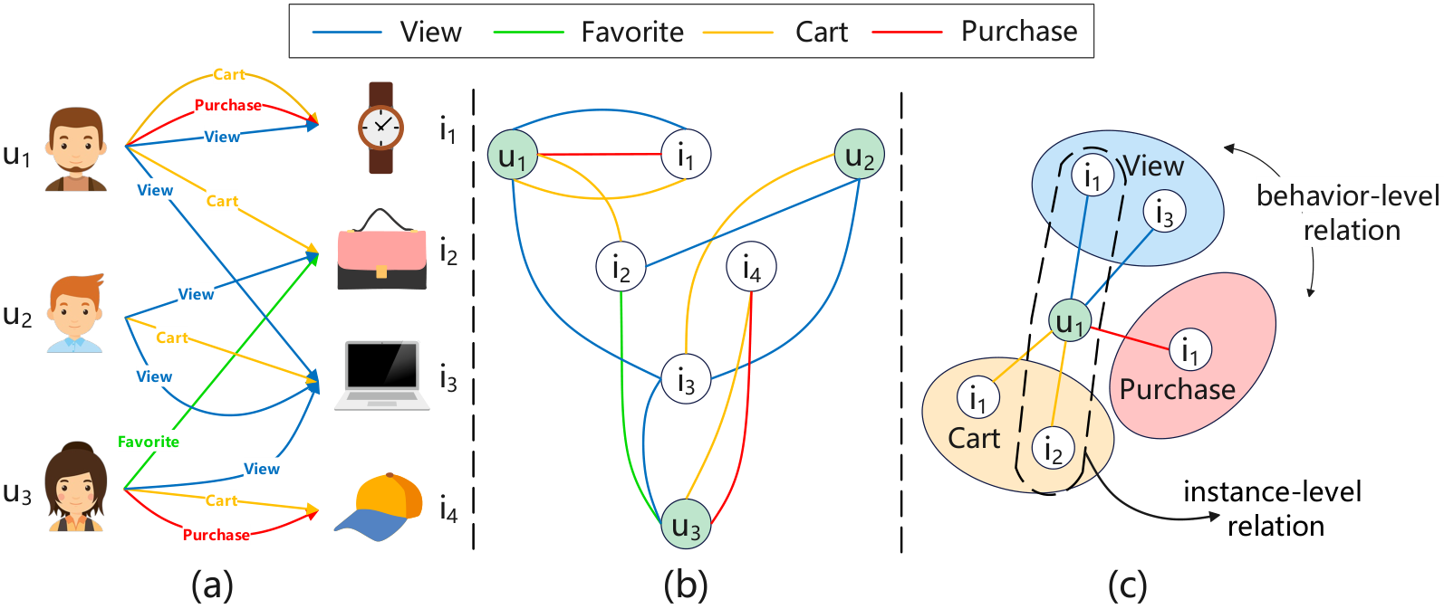
1. Introduction
Recommender systems (RS) serve as an important tool to meet personalized information needs. To predict users’ preferences for items, various methods have been devoted to Collaborative Filtering (CF) (Su and Khoshgoftaar 2009) techniques, which learn user and item representations from their historical interactions and then make predictions based on these representations. Most CF methods (Rendle et al. 2012; Xue et al. 2017; He et al. 2017; Wang et al. 2019a; He et al. 2020) are designed for a single type of behavior and rarely consider users’ multi-faceted preferences, which widely exist in real-world web applications. Take the example of an e-commerce website, as shown in Figure 1(a). Users interact with items through different behaviors, such as viewing, adding to cart, tagging as favorites, and purchasing. Since different types of behaviors exhibit different interactive patterns out of users’ diverse interests, it’s of great importance to explicitly leverage multi-behavior data for recommendation.
NMTR (Gao et al. 2019), DIPN (Guo et al. 2019), and MATN (Xia et al. 2020) regard multiple behaviors as different types and employ neural collaborative filtering unit, attention operator, and transformer architecture to model their dependencies, which perform much better than treating them as the same type. Multi-behavior data can be regarded as a multiplex bipartite graph (MBG), as shown in Figure 1(b). Recently, thanks to its capacity in representing relational information and modeling high-order relations which carry collaborative signals among users and items, graph neural networks (GNNs) based models (Wang et al. 2019a; He et al. 2020; Chen et al. 2020; Meng et al. 2022) have become popular for recommendation. For example, MBGCN (Jin et al. 2020), GHCF (Chen et al. 2021), and MB-GMN (Xia et al. 2021) further empower GNNs with multi-graph, non-sampling, and meta network to capture high-order collaborative signals on multiplex bipartite graphs.
Multi-behavior data can be treated “as features” for multi-behavior relation learning or “as labels” for multi-task supervised learning. Despite years of research, two challenges remain:
- •
Unbalanced Data Distribution. As we can see from Figure 2, observed interactions are highly unbalanced for different users and different behaviors, where a small percentage of users and behaviors cover most of the interactions.
- •
Sparse Target Behavior (behavior to be predicted, e.g., purchase in e-commerce). We can also find that most users have less than 10 purchase records, which is extremely sparse compared with the whole item space with thousands to millions of items.
We dig into these challenges and observe the following limitations:
- •
Inadequate modeling of high-order relations when treating multi-behavior data “as features”. User-item relations are meaningful for revealing the underlying reasons that motivate users’ preference on items. For example, as shown in Figure 1(a), there are several third order relations between and (e.g., ). With the help of collaborative effect, we predict that is likely to purchase as , the user similar to , has purchased before. Existing methods like MBGCN, GHCF, and MB-GMN have attempted to employ GNNs to incorporate high-order relations. However, they use a two-stage paradigm which first learns representation for each behavior by considering all historical records belonging to this behavior, then leveraging the learned representation to model high-order relation across different behaviors. We argue that this relation modeling manner is behavior-level, as depicted in Figure 1(c). Due to the unbalanced data distribution, the learned relations are easily biased toward high-degree users and behaviors, and thus making the learned representations unable to effectively capture high-order relations.
- •
Potential gradient conflict when treating multi-behavior data “as labels”. Early works like MBGCN (Jin et al. 2020) and MATN (Xia et al. 2020) only use target behavior as labels to train the model, which is vulnerable to the sparsity problem due to the sparse target behavior. To alleviate this problem, it is promising to use auxiliary behaviors as labels with multi-task learning (MTL) techniques. However, it is not easy to train with multiple objectives due to the negative transfer11 1 We ignore the seesaw phenomenon (i.e., MTL models improve the performances of some tasks while sacrifices the others) (Tang et al. 2020) here as the objective is to predict the target behavior in the multi-behavior recommendation. (Torrey and Shavlik 2010) phenomenon. Negative transfer indicates the performance deterioration when knowledge is transferred across different tasks. Therefore, it’s risky to treat multi-behavior data "as labels". Several recent works like NMTR (Gao et al. 2019), GHCF (Chen et al. 2021), and MB-GMN (Xia et al. 2021) have investigated MTL in multi-behavior recommendation. As they use the same input, these methods might suffer from the gradient conflict due to the coupled gradient issue. Detailed explanations are presented in Section 4.
To tackle the above limitations, we propose a novel Compressed Interaction Graph based Framework (CIGF) for better representation learning of users and items. To handle the inadequate modeling of high-order relations when treating multi-behavior data "as features", we design a Compressed Interaction Graph Convolution Network (CIGCN) to model high-order relations explicitly. CIGCN firstly leverages matrix multiplication as the interaction operator to generate high-order interaction graphs which encode instance-level high-order relations (including user-user, user-item, and item-item) explicitly, then leverages node-wise attention mechanism to select the most useful high-order interaction graphs and compress the graph space. Finally, state-of-the-art GCN models are combined with residual connections (He et al. 2016) on these graphs to explore high-order graph information and alleviate the over-smoothing issue for representation learning.
To alleviate the potential gradient conflict when treating multi-behavior data "as labels", we propose a Multi-Expert with Separate Input (MESI) network on the top of CIGCN for MTL. MESI network is a hierarchical neural architecture similar to the MMOE (Ma et al. 2018) and PLE (Tang et al. 2020). However, separate inputs are introduced to replace the same input used in the original MMOE and PLE models for MTL. Specifically, we use relations starting from different types of behaviors for the learning of separate inputs. By using separate inputs explicitly to learn task-aware information, potential gradient conflict of the same input can be alleviated when knowledge is transferred across different tasks, which makes the learning process more stable and effective. Explanations for the decoupled gradient of MESI can be referred to Section 4.
To summarize, our work makes the following contributions:
- •
We look at the multi-behavior recommendation problem from a new perspective, which treats multi-behavior data "as features" and "as labels" with data analysis and theoretical support.
- •
We propse a novel compressed Interaction Graph based Framework (CIGF) which is composed of a Compressed Interaction Graph Convolution Network (CIGCN) and a Multi-Expert with Separate Input (MESI) network. CIGCN is designed for instance-level high-order relation modeling with explicit graph interaction when treating multi-behavior data "as features". MESI is designed to alleviate the potential gradient conflict with separate inputs when treating multi-behavior data "as labels".
- •
We conduct extensive experiments on three real-world datasets to demonstrate the effectiveness of our proposed CIGF framework. The ablation analysis and in-depth analysis further verify the effectiveness and rationality of CIGCN and MESI. Besides, we further analyze the complexity of our method and conduct detailed efficiency experiments in Appendix A.6.
2. Related Work
GNNs for Recommendation.
GNNs based methods can be used for multi-behavior data by treating it “as features”.
Most of the existing GNNs are proposed for homogeneous graphs, such as NGCF (Wang
et al. 2019a), LR-GCCF (Chen
et al. 2020), and LightGCN (He
et al. 2020), which ignore the multiple types of edges.
Recently, some researchers have focused on the heterogeneous graph and proposed methods like HGNN (Zhang
et al. 2019), R-GCN (Schlichtkrull et al. 2018), and HGAT (Linmei
et al. 2019).
However, these methods merely consider the behavior-level relations by utilizing the behavior-level representations for relation modeling.
Hyper-graph based methods (Feng
et al. 2019; Benson
et al. 2016) leverage hyper-graph to model complex high-order
relations.
However, as an edge in hyper-graph connects two or more nodes, it is not suitable for the multi-behavior case where a node pair connects multiple edges.
Existing meta-path based methods, like Metapath2vec (Dong
et al. 2017), MCRec (Hu
et al. 2018), and HAN (Wang
et al. 2019b) model high-order relations with the manually selected meta-paths, which is limited by the need of expert knowledge and the difficulty of searching all useful meta-paths with arbitrary length and edge types.
MTL for Recommendation.
MTL methods can be used for multi-behavior data by treating it “as labels”.
A widely used model is the shared bottom structure in Figure 3(d).
Though useful for knowledge sharing within multiple tasks, it still suffers from the risk of conflicts due to the task differences.
To handle the task difference, some studies apply the attention network for information fusion.
MMOE (Ma
et al. 2018) in Figure 3(e) extends MOE (Jacobs
et al. 1991) to utilize different gating networks to obtain different fusion weights in MTL.
PLE (Tang
et al. 2020) in Figure 3(f) further proposes to leverage shared or task-specific experts at the bottom and then employs gating networks to combine these experts adaptively, thus to handle task conflicts and alleviate the negative transfer issue.
However, they still utilize the same input for MTL.
We argue that this manner might suffer from the gradient conflict due to the coupled gradient issue.
Detailed explanations are presented in Section 4.
Multi-behavior Recommendation.
Existing multi-behavior recommendation methods can be classified into two categories: graph-based and MTL based (Huang 2021).
The former category treats multi-behavior data “as features”.
Some early works like DIPN (Guo
et al. 2019) and MATN (Xia
et al. 2020) fail to capture high-order relations, and thus performing poor.
Most recent works (e.g., GHCF (Chen et al. 2021) and MBGCN (Jin
et al. 2020)) use a behavior-level modeling manner that cannot capture the fine-grained instance-level multi-behavior relations.
Some other methods like MBGCN (Jin
et al. 2020) and MGNN (Zhang
et al. 2020) learn high-order relations from the MBG directly, which is difficult to mine useful relations extensively due to the unbalanced data distribution.
Different from the above methods, our proposed CIGCN models high-order relation by explicit graph interaction and graph compression, thus can learn relations in the instance-level.
The latter category treats multi-behavior data “as labels”.
NMTR (Gao et al. 2019) in Figure 3(a) assumes that users’ multiple types of behaviors take place in a fixed order, which may be too strong to be appropriate for all users.
GHCF in Figure 3(b) uses a similar architecture with shared bottom for MTL.
The only difference is that GHCF uses bilinear operation (Please refer to Section 4) as the prediction head, while shared bottom uses neural network.
MB-GMN (Xia
et al. 2021) in Figure 3(c) further proposes to use a meta prediction network to capture the complex cross-type behavior dependency for MTL.
These existing methods optimize multiple tasks with the same static weights for all samples.
The most obvious drawback is that they can easily suffer from the risk of conflicts caused by sample differences, as different samples may pose different preferences for different tasks.
In contrast, our proposed MESI network learns adaptive weights according to the nature of different samples.
Besides, we utilize the separate input to learn task-aware information to alleviate the potential gradient conflict.
3. Preliminary
3.1. Problem Definition
In this section, we give the formal definition of the multi-behavior recommendation task. We denote the user set and item set as and , respectively. The user-item interaction matrices of behaviors as . Where , and are the number of users, items and behavior types, respectively, and denotes that user interacts with item under behavior , otherwise . Generally, there is a target behavior to be optimized (e.g., purchase), which we denote as , and other behaviors (e.g., view and tag as favorite) are treated as auxiliary behaviors for assisting the prediction of target behavior. The goal is to predict the probability that user will interact with item under target behavior .
3.2. Graph and Relation Definition
As shown in Figure 1(b), we denote the Multiplex Bipartite Graph (MBG) as , where is the node set containing all users and items, is the edge set including all behavior records between users and items. Here denotes a specific type of behavior and is the set of all possible behavior types. is the adjacency matrix set with denoting adjacency matrix of a specific behavior graph .
A relation is defined as a path in the MBG with the form of . We denote as the set of all edge types in this path. If and , we define this path as a high-order single-behavior relation. If and , we define this path as a high-order multi-behavior relation. Node is node ’s -th order reachable neighbor if there exists a path connecting node and node and the length of this path is . In a new generated graph , if arbitrary two connected nodes and are -th order reachable in the original MBG , is defined as a -th order graph. We will illustrate the explicitly modeling of high-order multi-behavior relation through high-order graph interaction and convolution in Section 4.2.
3.3. A Coupled Gradient Issue in MTL
Most of the existing methods use the same input for MTL, as summarized in Section 2. This may cause a coupled gradient issue in MTL which restricts their learning ability for each task. Here we use bilinear module from GHCF (Chen et al. 2021) as an example to claim this. The bilinear module can be formulated as:
| (1) |
where () is the hadamard product operation, denotes the predictive value of the k-th behavior, and represent the learned representation for user and item . is a behavior-aware transformation vector, which projects user and item representation to separate prediction head for MTL, and denotes the embedding size. Here we use the square loss as an example for optimization:
| (2) |
where is the true label. Then we have:
| (3) |
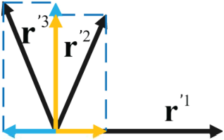
where is an scalar, is the synthetic gradient from the -th behavior, which determines the updating magnitude and direction of the same input vector . We can see that the gradients from all behaviors are coupled. Figure 4 shows an example of . Assuming as a reference vector, we do orthogonal decomposition to all the other vectors. We can find that the components of other vectors are not in the same direction as the reference vector. This demonstrates the potential gradient conflict brought by the coupled gradient. The proof for other methods, loss functions and the decoupled gradient of MESI can be referred to Appendix A.2 and A.3.
4. Our Proposed Method
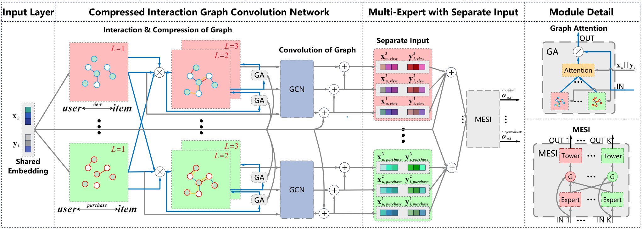
We now present the proposed CIGF framework, which treats multi-behavior data both “as features” and “as labels” in an end-to-end fashion. The architecture is shown in Figure 5 and it consists of three main components: i) input layer, which parameterizes users and items as embedding vectors; ii) compressed interaction graph convolution network (CIGCN), which extracts instance-level high-order relation from the multi-behavior data explicitly by treating it “as features”; iii) multi-expert with separate input (MESI) network, which mines multi-task supervision signals from the multi-behavior data with separate inputs by treating it “as labels”.
4.1. Input
We first apply a shared embedding layer to transform the one-hot IDs of users and items into low-dimensional dense embeddings. Formally, given a user-item pair , the embedding lookup operation for user and item can be formulated as follows:
| (4) |
where and denotes the one-hot IDs of user and item , and are the user and item embedding matrix and is the embedding size.
4.2. Compressed Interaction Graph Convolution
4.2.1. Graph Interaction
Inspired by the success of DCN (Wang et al. 2017) and xDeepFM (Lian et al. 2018) which model high-order feature interactions with explicit feature crossing, we use the adjacency matrix multiplication as the graph interaction operator for explicit instance-level high-order relation modeling. As shown in Figure 5, we first partition the MBG into several behavior-specified graph . The corresponding adjacency matrices are , which can be formulated as:
| (5) |
where is the user-item interaction matrix of behavior . We then use these adjacency matrices for explicit high-order graph interaction which encodes the instance-level relations of each two nodes. Denote the set of all possible -th () order interaction graph starting from behavior as . The purpose why we only use interaction graph starting from behavior here is to generate graph sets with different high-order relations, which will be used as separate inputs for MESI to alleviate the potential gradient conflict. The generation of can be formulated as:
| (6) |
where . () denotes the matrix multiplication operation between any pairs of matrices from the two sets separately. Noticed that there are sets of high-order graph , each of which starts from a behavior-specified adjacency matrix . By selecting different behavior-specific graph at each step, we can construct a high-order graph set that contains multiple -th order interaction graph with different semantics. Specifically, the number of all possible -th order graph can be calculated as:
| (7) |
where is a measure of the number of elements in a set, is the function that calculates the power of a given number , is the number of behavior types. However, as the number of all possible -th order graph is a exponential function of , it’s impractical to use such an extensive space for -order interaction graph generation.
4.2.2. Graph Compression.
In order to find an applicable solution with limited time and space complexity, we employ a graph compression layer to construct the high-order graph sets iteratively with the node-wise multi-head attention mechanism. The graph compression layer for target node (node could be a user node or an item node ) can be formulated as:
| (8) |
where . is the vector multiplication operation, is the number of heads and is the learned attention vector for node in the -th order and the -th head. By using the node-wise multi-head attention mechanism, the number of generated -th order graph is reduced from to . Since is usually much smaller than and is usually a very small value, so the scale of is acceptable. The attention mechanism not only serves as a tool to reduce complexity, but is also used for finding the most useful behaviors for high-order graph generation. To adaptively select the most relevant behavior of users and items for representation learning, we use the node-wise attention mechanism to obtain the soft weights for different behaviors, which can be defined as:
| (9) |
where is the activation function set as LeakyReLU here for better performance. and are feature transformation matrix and bias matrix, respectively. Noticed that we also use a behavior- and layer-wise (i.e., we use different transformation matrices for different layers and behaviors) attention mechanism here, we empirically verify its effectiveness in Section 5.3.1. In this way, we can generate the personalized high-order graph sets for both users and items, which are used for later information propagation and integration.
4.2.3. Graph Convolution
After generating the graph set by graph interaction and graph compression layers, we enrich the representation of users and items with graph convolution. The neighbor information propagation in each graph can be formulated as:
| (10) |
where and denote the adjacent matrices of the -th and -th graph in graph set and , and denote the neighbors of and , and and denote the outputs by aggregating neighbor information from -th and -th graph. is a arbitrary graph convolution operator that can be used for information aggregation. We implement with the following four state-of-the-art GCN models: GCN Aggregator (Kipf and Welling 2016), NGCF Aggregator (Wang et al. 2019a), LR-GCCF Aggregator (Chen et al. 2020), and LightGCN Aggregator (He et al. 2020). Notice that the matrix multiplications lead to a very dense high-order graph which is computationally unacceptable. Therefore, we use the matrix associative property to accelerate the aggregation process for computational efficiency. For example, can be accelerated by , where ( is the multiplication between sparse matrix and vector. As ( combines a sparse matrix and a vector into a single vector, computation complexities of subsequent multiplications can be effectively reduced. After the neighbor information propagation process, we have neighbor representations for each layer and for each node and . For simplicity, we apply the sum operation over these representations to get the final user and item representations:
| (11) |
To better explore high-order neighbor information and alleviate the over-smoothing issue, we introduce the residual operation to our graph convolution layer for final node information updating, which is defined as:
| (12) |
As the outputs of different layers reflects the relations of different orders, we finally aggregate these outputs into a single vector with the sum operation as follows:
| (13) |
where and are the initial embeddings for user and item . It is noticed that the central nodes aggregate neighbor information of different layers directly, which has been verified to be useful to address the heterogeneity of the user-item interaction graph (Sun et al. 2020), compared with recursively updating the node embedding at -th layer with the output from -th layer.
4.3. Multi-Expert with Separate Input
With the design of CIGCN, we have obtained representations and for each user and each item , as shown in Figure 5. Each representation describes the personalized preferences of user or item to relations start from behavior . To alleviate the potential gradient conflict when treating multi-behavior data "as labels", we propose a Multi-Expert with Separate Input (MESI) network with a novel separate input design in this section.
Existing multi-behavior methods like NMTR (Gao et al. 2019), GHCF (Chen et al. 2021) and MB-GMN (Xia et al. 2021) optimize multiple tasks with the same static weights for all samples, which are limited by the sample differences, as analyzed in Section 2. To address this problem, we use a hierarchical neural architecture which is similar to the MMOE (Ma et al. 2018) and PLE (Tang et al. 2020) for MTL. Specifically, we use experts to replace the shared bottom layer used in NMTR, GHCF and MB-GMN to learn behavior-aware information. In this paper, each expert is defind as the combination of and , which can be formulated as:
| (14) |
where () is the hadamard product operation, and are the behavior related inputs. As the separate input are utilized here for the generation of experts, we can obtain experts in total.
As different experts may contain different preferences of users or properties of items, it’s necessary to combine these experts for the final prediction of each task. We then use the separate input to produce task-aware gate for each task to automatically select a subset of experts which are useful for the prediction of this task. The gate for task can be defined as:
| (15) |
where is the vector concatenation operation, and are feature transformation matrix and bias matrix, and is the attention vector which are used as selector to calculate the weighted sum of all experts. The final prediction score for task is calculated as:
| (16) |
where denotes the -th element of vector , is the tower function. Following (Jacobs et al. 1991), we use average operation as the tower function here for simplicity.
4.4. Joint Optimization for MTL
Since we have obtained the prediction value for each type of behavior , we use the Bayesian Personalized Ranking (BPR) (Rendle et al. 2012) loss for multi-task learning, which can be formulated as:
| (17) |
where denotes the training dataset. indicates observed positive user-item interactions under behavior and indicates unobserved user-item interactions under behavior . represents set of all model parameters, is the Sigmoid function and is the regularization coefficient for .
| Dataset | User | Item | Interaction | Behaviors |
|---|---|---|---|---|
| Beibei | 21,716 | 7,977 | 3,338,068 | View,Cart,Buy |
| Taobao | 147,894 | 99,037 | 7,658,926 | View,Favorite,Cart,Buy |
| IJCAI | 423,423 | 874,328 | 36,203,512 | View,Favorite,Cart,Buy |
5. EXPERIMENTS
5.1. Experiment Setup
5.1.1. Datasets
To reduce biases, we adopt the same public datasets (i.e., Beibei, Taobao, and IJCAI)22 2 https://github.com/akaxlh/MB-GMN and pre-processings as in MB-GMN (Xia et al. 2021), and the statistics are shown in Table 1.
5.1.2. Compared Baseline
For a comprehensive comparison, we compare CIGF against four types of representative baselines: i) NNs-based single-behavior models, i.e., DMF (Xue et al. 2017) and AutoRec (Sedhain et al. 2015); ii) NNs-based multi-behavior models, i.e., NMTR (Gao et al. 2019), DIPN (Guo et al. 2019), and MATN (Xia et al. 2020); iii) GNNs-based single-behavior models, i.e., NGCF (Wang et al. 2019a) and LightGCN (He et al. 2020); iv) GNNs-based multi-behavior models, i.e., NGCFM (Wang et al. 2019a), LightGCNM (LightGCN (He et al. 2020) enhanced with the multi-behavioral graph), GHCF (Chen et al. 2021), and MBGCN (Jin et al. 2020). Public codes for GHCF33 3 https://github.com/chenchongthu/GHCF; Due to the unaffordable memory usage brought by non-sampling learning, GHCF is inapplicable to the IJCAI dataset. and LightGCN44 4 https://github.com/kuandeng/LightGCN are used, while the best results for other models (DMF, AutoRec, NGCF, NMTR, DIPN, MATN, MBGCN, and MB-GMN) are picked from (Xia et al. 2021).
5.1.3. Evaluation Metrics
The Hit Ratio (HR@) and Normalized Discounted Cumulative Gain (NDCG@) are used to evaluate the performances. By default, we set in all experiments. Similar results of other metrics (i.e., ) on the three datasets can also be obtained, whereas they are not presented here due to the space limitation. And the details of implementation are shown in Appendix A.1.
5.2. Overall Performance Comparison
From Table 2, we have the following observations in terms of model effectiveness (analysis of complexity is shown in Appendix A.6):
| Dataset | Beibei | Taobao | IJCAI | |||
| Model | HR | NDCG | HR | NDCG | HR | NDCG |
| DMF | 0.597 | 0.336 | 0.305 | 0.189 | 0.392 | 0.250 |
| AutoRec | 0.607 | 0.341 | 0.313 | 0.190 | 0.448 | 0.287 |
| NGCF | 0.611 | 0.375 | 0.302 | 0.185 | 0.461 | 0.292 |
| LightGCN | 0.643 | 0.378 | 0.373 | 0.235 | 0.443 | 0.283 |
| NMTR | 0.613 | 0.349 | 0.332 | 0.179 | 0.481 | 0.304 |
| DIPN | 0.631 | 0.394 | 0.317 | 0.178 | 0.475 | 0.296 |
| MATN | 0.626 | 0.385 | 0.354 | 0.209 | 0.489 | 0.309 |
| NGCFM | 0.634 | 0.372 | 0.374 | 0.221 | 0.481 | 0.307 |
| LightGCNM | 0.651 | 0.391 | 0.391 | 0.243 | 0.486 | 0.317 |
| GHCF | 0.608 | 0.378 | 0.415 | 0.241 | - | - |
| MBGCN | 0.642 | 0.376 | 0.369 | 0.222 | 0.463 | 0.277 |
| MB-GMN | 0.691 | 0.410 | 0.491 | 0.300 | 0.532 | 0.345 |
| CIGF | ||||||
| %Improv | 1.30% | 8.05% | 20.57% | 27.67% | 12.97% | 15.94% |
- •
CIGF consistently yields superior performance on all three datasets. More precisely, CIGF outperforms the strongest baselines by 1.30%, 20.57%, and 12.97% in terms of HR (8.05%, 27.67%, and 15.94% in terms of NDCG) on Beibei, Taobao, and IJCAI, respectively. Additionally, the performance improvements on Taobao and Ijcai datasets are much more significant than that on Beibei dataset. One possible reason is that the interaction information of different behaviors contained in Beibei dataset is mutually covered (as shown in Appendix 10, users who have bought an item must also have viewed and carted it), which reduces the significance of high-order relation modeling.
- •
NGCF and LightGCN perform better than DMF and AutoRec on most datasets, which demonstrates the advantage of GNN in extracting high-order collaborative signals. By distinguishing different behaviors, NMTR, DIPN, and MATN achieve much better performances than DMF and AutoRec. This verifies the necessity to extract and model the relation information between different types of behaviors.
- •
NGCF, LightGCN, NMTR, DIPN, and MATN perform worse than NGCFM, LightGCNM, MBGCN, and MB-GMN on most datasets, which indicates the incapability of NNs models and single-behavior GNNs models in modeling high-order multi-behavior relations. This justifies the necessity to simultaneously consider multi-behavior and high-order relations.
5.3. Ablation Study of CIGF
5.3.1. On the effectiveness of key components
| Dataset | Beibei | Taobao | IJCAI | |||
|---|---|---|---|---|---|---|
| Model | HR | NDCG | HR | NDCG | HR | NDCG |
| Base Model | 0.649 | 0.392 | 0.444 | 0.275 | 0.457 | 0.297 |
| w/o CIGCN | 0.660 | 0.410 | 0.460 | 0.286 | 0.495 | 0.322 |
| w/o MESI | 0.662 | 0.401 | 0.528 | 0.340 | 0.573 | 0.382 |
| CIGF | 0.700 | 0.443 | 0.592 | 0.383 | 0.601 | 0.400 |
To evaluate the effectiveness of sub-modules in our CIGF framework, we consider three model variants: (1) Base Model: We remove CIGCN part (i.e., the behavior-specific graph are used for convolution directly) and replace the MESI network with bilinear module. This variant cannot model instance-level high-order relations and use same input for MTL. (2) w/o CIGCN: The CIGCN part is removed. (3) w/o MESI: The MESI part is replaced with bilinear module. As shown in Table 3, both CIGCN and MESI bring performance improvements compared with base model, and the complete CIGF framework achieves the best results. Therefore, we claim that both instance-level high-order multi-behavior relation and separate input are effective and complementary to each other. And it’s necessary to treat multi-behavior data both "as features" and "as labels".
| Dataset | Beibei | Taobao | IJCAI | |||
|---|---|---|---|---|---|---|
| Method | HR | NDCG | HR | NDCG | HR | NDCG |
| global-wise | 0.694 | 0.438 | 0.565 | 0.361 | 0.572 | 0.373 |
| node-wise | 0.698 | 0.442 | 0.561 | 0.356 | 0.587 | 0.390 |
| node-wise+layer | 0.698 | 0.442 | 0.564 | 0.361 | 0.590 | 0.392 |
| node-wise+beh | 0.698 | 0.441 | 0.588 | 0.379 | 0.599 | 0.398 |
| node-wise+beh+layer | 0.700 | 0.443 | 0.592 | 0.383 | 0.601 | 0.400 |
5.3.2. On the impact of attention module.
To demonstrate the effectiveness of our attention module, we consider four variants: (1) global-wise: The attention weight is global-wise for all user/item. (2) node-wise: The attention weight is shared by all layers and behaviors but different for each user/item. (3) node-wise+layer: The attention weight is shared by all behaviors but different for each layer or user/item. (4) node-wise+beh: The attention weight is shared by all layers but different for each behavior or user/item. From the results displayed in Table 4, global-wise attention performs the worst among all variants in most cases, which suggests the importance of learning the customized information for each node. Besides, all the enhanced node-wise variants perform better than pure node-wise attention mechanism, and our proposed attention mechanism achieves the best performance on all three datasets. The results indicate the effectiveness and rationality of our proposed behavior-wise and layer-wise node-wise attention mechanism for high-order multi-behavior relation selection.
5.3.3. On the impact of MTL modules.
| Dataset | Beibei | Taobao | IJCAI | |||
|---|---|---|---|---|---|---|
| Method | HR | NDCG | HR | NDCG | HR | NDCG |
| CIGCN-SB | 0.605 | 0.341 | 0.389 | 0.231 | 0.485 | 0.302 |
| CIGCN-Bilinear | 0.662 | 0.401 | 0.528 | 0.340 | 0.573 | 0.382 |
| CIGCN-MMOE | 0.663 | 0.391 | 0.541 | 0.338 | 0.546 | 0.339 |
| CIGCN-PLE | 0.653 | 0.381 | 0.521 | 0.320 | 0.526 | 0.325 |
| CIGF | 0.700 | 0.443 | 0.592 | 0.383 | 0.601 | 0.400 |
To further demonstrate the superiority of our proposed MESI for MTL, we replace it with four state-of-the-art MTL modules, namely, Shared Bottom (Caruana 1997), Bilinear (Chen et al. 2021), MMOE (Ma et al. 2018), and PLE (Tang et al. 2020), and apply them on the top of CIGCN for multi-behavior recommendation. Notice that there are representations used as separate input generated from CIGCN. To make it applicable for these four modules which use same input, we average the representations to get one unified input. Resulted variants are named as CIGCN-SB, CIGCN-Bilinear, CIGCN-MMOE, CIGCN-PLE, and CIGF respectively. The results are summarized in Table 5. As we can see, CIGCN-SB performs the worst among all MTL models on all datasets. CIGCN-Bilinear replaces the prediction head of neural network in CIGCN-SB with lightweight matrix transformation and performs better. Possible reason is that the lightweight operation can reduce the risk of overfitting. Besides, both CIGCN-MMOE and CIGCN-PLE have employed the gate network with adaptive attention weights for information fusing, thus outperform the static and same-weighted CIGCN-SB. Finally, our MESI consistently performs the best on all datasets. This verifies the effectiveness of separate input for MTL.
5.3.4. On the impact of GCN aggregators.
To explore the impact of different GCN aggregators, we compare the variants of our proposed model with different GCN aggregators, including GCN Aggregator (Kipf and Welling 2016), NGCF Aggregator (Wang et al. 2019a), LR-GCCF Aggregator (Chen et al. 2020), and LightGCN Aggregator (He et al. 2020). The experimental results are illustrated in Figure 6. We can see that NGCF Aggregator performs better than GCN aggregators on all datasets. A possible reason is that additional feature interactions introduced by NGCF Aggregator provides more information. We also find that LR-GCCF Aggregator performs slightly better than NGCF Aggregator on almost all datasets. The reason is that removing the transformation matrix can alleviate overfitting. Moreover, LightGCN Aggregator obtains the best performance on all datasets by simultaneously removing transformation matrix and activation function.
5.4. In-depth Analysis of Model Design
In this part, we conduct experiments to make in-depth analysis about instance-level high-order relation modeling when treating multi-behavior data "as features" and potenial gradient conflict when treating multi-behavior data "as labels".
5.4.1. Instance-level high-order relation modeling.
We vary the depth of CIGF to investigate whether our model can benefit from instance-level high-order relations. And we compare the results with GHCF and MB-GMN which model behavior-level high-order relations. Due to lack of space, we only show the results on Beibei and Taobao datasets in Figure 7, the result of another dataset is consistent. We can see that CIGF consistently outperforms the other methods when the layer number increases. Besides, we can also find CIGF keeps stable on Beibei and increases continuously on Taobao, while MBGCN degrades rapidly on both datasets and GHCF degrades rapidly on Beibei when increasing the layer number. This observation verifies the effectiveness of our proposed method for instance-level high-order relation modeling.
| Dataset | Relation | Second order | Third order | Fourth order |
|---|---|---|---|---|
| Beibei | top-3 | CC, CV, PP | - | - |
| bottom-3 | CP, PV, VP | - | - | |
| Taobao | top-3 | FP, CP, PC | FPP, CPP, PCP | PFFP, CFFP, FPPV |
| bottom-3 | PP, CC, FF | PPP, PPV, PPF | PPPF, PPPC, PPPP | |
| IJCAI | top-3 | CV, FV, PV | PVV, CVV, FFF | PVPV, CPPV, CVPV |
| bottom-3 | FC, CC, PC | FCF, CCF, FCP | FCFC, CCFC, PCFC |
Instance-level high-order relations bring benefits for final recommendation. Besides, it can also reveal the underlying reasons that motivate users’ preferences on items. Towards this end, we select and show the top-3 and bottom-3 relations among all possible relations for each order according to the average attention weights of all users in Table 6. Notice that there are only second order relations on Beibei as our model achieves best results with two layers on this dataset. As we can see, the third order relation has the highest average attention weights on Taobao. Possible explanation is that users tend to purchase items bought by similar users. Besides, the second order relation has the lowest average attention weights on IJCAI. The rationality can be verified in Appendix 10 that the probability that users only have favor and cart behaviors with the same items is zero on IJCAI.
5.4.2. Gradient conflict analysis.
To verify that our model can alleviate potential gradient conflict, we perform experiments on user groups with different behavior relevance levels. In particular, we divide the test set into six user groups according to the average Pearson correlation (Berthold and Höppner 2016) among all behaviors. The calculation of average Pearson correlation can be referred to Appendix A.4. For fair comparison, we select a subset from each user group to keep the interaction number for each user fixed, thus preventing the potential impact of node degree to results (Wang et al. 2019a). Figure 8 presents the results. We omit the results on the IJCAI dataset due to space limitation, which have consistent trends. For more rigorous results, we run each experiment 5 times and draw the mean and fluctuation range on the figure. We find that MESI consistently outperforms all baselines among all user groups, which further demonstrates the superiority of MESI for MTL. Besides, with the increase of behavior correlations, MESI gets better performances, while the performances of other baselines fluctuate or even decrease. A possible reason is the negative transfer caused by potential gradient conflict when knowledge is transferred across different tasks.
To understand the reason why our proposed MESI can alleviate potential gradient conflict, we conduct experiments to compare the experts utilization among our MESI and other gate-based models (MMOE and PLE). Following (Tang et al. 2020), we visualize the average weight distribution of experts used by the target behavior prediction in Figure 9. Notice that we omit gates used for other behaviors as our goal is to predict the interaction probability of target behavior. Besides, for the sake of comparison, we fix the number of experts as 3 on Beibei dataset and 4 on Taobao and IJCAI datasets for both MMOE and PLE. It is shown that our MESI achieves better differentiation between different experts while MMOE and PLE have a nearly uniform distribution for all experts. Thus our MESI can selectively leverage information of different behaviors to update the gradient to avoid potential conflict.
6. Conclusions
In this paper, we propose the CIGF framework for multi-behavior recommendations. To explicitly model instance-level high-order relations, we introduce the CIGCN module, which leverages matrix multiplication as the interaction operator to generate high-order interaction graphs, and perform graph convolution on these graphs to explore relation integration. To alleviate potential gradient conflict, we propose the MESI network, which uses behavior-specific separate inputs explicitly. By doing so, the risk of negative transfer is reduced. We conduct comprehensive experiments on three real-world datasets and show that the proposed CIGF outperforms all the state-of-the-art methods on all three datasets. Further analysis shows that CIGF can fully capture high-order relationships and effectively alleviate negative transfer.
Acknowledgements.
This work was partly supported by the Science and Technology Innovation 2030-Key Project under Grant 2021ZD0201404 and Aminer· ShenZhen·ScientificSuperBrain. And we thank MindSpore (min 2020) for the partial support of this work, which is a new deep learning computing framework.References
- (1)
- min (2020) 2020. MindSpore. https://www.mindspore.cn
- Abadi et al. (2016) Martín Abadi, Paul Barham, Jianmin Chen, Zhifeng Chen, Andy Davis, Jeffrey Dean, Matthieu Devin, Sanjay Ghemawat, Geoffrey Irving, Michael Isard, et al. 2016. TensorFlow: A System for Large-Scale Machine Learning. In 12th USENIX symposium on operating systems design and implementation (OSDI 16). 265–283.
- Benson et al. (2016) Austin R Benson, David F Gleich, and Jure Leskovec. 2016. Higher-order organization of complex networks. Science 353, 6295 (2016), 163–166.
- Berthold and Höppner (2016) Michael R Berthold and Frank Höppner. 2016. On clustering time series using euclidean distance and pearson correlation. arXiv preprint:1601.02213 (2016).
- Caruana (1997) Rich Caruana. 1997. Multitask learning. Machine learning 28, 1 (1997), 41–75.
- Chen et al. (2021) Chong Chen, Weizhi Ma, Min Zhang, Zhaowei Wang, Xiuqiang He, Chenyang Wang, Yiqun Liu, and Shaoping Ma. 2021. Graph Heterogeneous Multi-Relational Recommendation. In AAAI, Vol. 35. 3958–3966.
- Chen et al. (2020) Lei Chen, Le Wu, Richang Hong, Kun Zhang, and Meng Wang. 2020. Revisiting Graph Based Collaborative Filtering: A Linear Residual Graph Convolutional Network Approach. In AAAI, Vol. 34. 27–34.
- Dong et al. (2017) Yuxiao Dong, Nitesh V Chawla, and Ananthram Swami. 2017. metapath2vec: Scalable representation learning for heterogeneous networks. In SIGKDD.
- Feng et al. (2019) Yifan Feng, Haoxuan You, Zizhao Zhang, Rongrong Ji, and Yue Gao. 2019. Hypergraph neural networks. In AAAI, Vol. 33. 3558–3565.
- Gao et al. (2019) Chen Gao, Xiangnan He, Dahua Gan, Xiangning Chen, Fuli Feng, Yong Li, Tat-Seng Chua, and Depeng Jin. 2019. Neural multi-task recommendation from multi-behavior data. In ICDE. IEEE, 1554–1557.
- Glorot and Bengio (2010) Xavier Glorot and Yoshua Bengio. 2010. Understanding the difficulty of training deep feedforward neural networks. In AISTATS. 249–256.
- Guo et al. (2019) Long Guo, Lifeng Hua, Rongfei Jia, Binqiang Zhao, Xiaobo Wang, and Bin Cui. 2019. Buying or browsing?: Predicting real-time purchasing intent using attention-based deep network with multiple behavior. In SIGKDD. 1984–1992.
- He et al. (2016) Kaiming He, Xiangyu Zhang, Shaoqing Ren, and Jian Sun. 2016. Deep residual learning for image recognition. In CVPR. 770–778.
- He et al. (2020) Xiangnan He, Kuan Deng, Xiang Wang, Yan Li, Yongdong Zhang, and Meng Wang. 2020. LightGCN: Simplifying and Powering Graph Convolution Network for Recommendation. arXiv preprint arXiv:2002.02126 (2020).
- He et al. (2017) Xiangnan He, Lizi Liao, Hanwang Zhang, Liqiang Nie, Xia Hu, and Tat-Seng Chua. 2017. Neural collaborative filtering. In WWW. 173–182.
- Hu et al. (2018) Binbin Hu, Chuan Shi, Wayne Xin Zhao, and Philip S Yu. 2018. Leveraging meta-path based context for top-n recommendation with a neural co-attention model. In SIGKDD. 1531–1540.
- Huang (2021) Chao Huang. 2021. Recent Advances in Heterogeneous Relation Learning for Recommendation. arXiv preprint arXiv:2110.03455 (2021).
- Jacobs et al. (1991) Robert A Jacobs, Michael I Jordan, Steven J Nowlan, and Geoffrey E Hinton. 1991. Adaptive mixtures of local experts. Neural computation 3, 1 (1991), 79–87.
- Jin et al. (2020) Bowen Jin, Chen Gao, Xiangnan He, Depeng Jin, and Yong Li. 2020. Multi-behavior recommendation with graph convolutional networks. In SIGIR.
- Kingma and Ba (2014) Diederik P Kingma and Jimmy Ba. 2014. Adam: A method for stochastic optimization. arXiv preprint arXiv:1412.6980 (2014).
- Kipf and Welling (2016) Thomas N Kipf and Max Welling. 2016. Semi-supervised classification with graph convolutional networks. arXiv preprint arXiv:1609.02907 (2016).
- Lian et al. (2018) Jianxun Lian, Xiaohuan Zhou, Fuzheng Zhang, Zhongxia Chen, Xing Xie, and Guangzhong Sun. 2018. xdeepfm: Combining explicit and implicit feature interactions for recommender systems. In SIGKDD. 1754–1763.
- Linmei et al. (2019) Hu Linmei, Tianchi Yang, Chuan Shi, Houye Ji, and Xiaoli Li. 2019. Heterogeneous graph attention networks for semi-supervised short text classification. In EMNLP-IJCNLP. 4821–4830.
- Ma et al. (2018) Jiaqi Ma, Zhe Zhao, Xinyang Yi, Jilin Chen, Lichan Hong, and Ed H Chi. 2018. Modeling task relationships in multi-task learning with multi-gate mixture-of-experts. In SIGKDD. 1930–1939.
- Meng et al. (2022) Chang Meng, Ziqi Zhao, Wei Guo, Yingxue Zhang, Haolun Wu, Chen Gao, Dong Li, Xiu Li, and Ruiming Tang. 2022. Coarse-to-Fine Knowledge-Enhanced Multi-Interest Learning Framework for Multi-Behavior Recommendation. arXiv preprint arXiv:2208.01849 (2022).
- Rendle et al. (2012) Steffen Rendle, Christoph Freudenthaler, Zeno Gantner, and Lars Schmidt-Thieme. 2012. BPR: Bayesian personalized ranking from implicit feedback. arXiv preprint arXiv:1205.2618 (2012).
- Schlichtkrull et al. (2018) Michael Schlichtkrull, Thomas N Kipf, Peter Bloem, Rianne Van Den Berg, Ivan Titov, and Max Welling. 2018. Modeling relational data with graph convolutional networks. In European semantic web conference. Springer, 593–607.
- Sedhain et al. (2015) Suvash Sedhain, Aditya Krishna Menon, Scott Sanner, and Lexing Xie. 2015. Autorec: Autoencoders meet collaborative filtering. In WWW. 111–112.
- Su and Khoshgoftaar (2009) Xiaoyuan Su and Taghi M Khoshgoftaar. 2009. A survey of collaborative filtering techniques. Advances in artificial intelligence 2009 (2009).
- Sun et al. (2020) Jianing Sun, Yingxue Zhang, Wei Guo, Huifeng Guo, Ruiming Tang, Xiuqiang He, Chen Ma, and Mark Coates. 2020. Neighbor interaction aware graph convolution networks for recommendation. In SIGIR. 1289–1298.
- Tang et al. (2020) Hongyan Tang, Junning Liu, Ming Zhao, and Xudong Gong. 2020. Progressive layered extraction (ple): A novel multi-task learning (mtl) model for personalized recommendations. In RecSys. 269–278.
- Torrey and Shavlik (2010) Lisa Torrey and Jude Shavlik. 2010. Transfer learning. In Handbook of research on machine learning applications and trends: algorithms, methods, and techniques. IGI global, 242–264.
- Wang et al. (2017) Ruoxi Wang, Bin Fu, Gang Fu, and Mingliang Wang. 2017. Deep & cross network for ad click predictions. In Proceedings of the ADKDD’17. 1–7.
- Wang et al. (2019a) Xiang Wang, Xiangnan He, Meng Wang, Fuli Feng, and Tat-Seng Chua. 2019a. Neural graph collaborative filtering. In SIGIR. 165–174.
- Wang et al. (2019b) Xiao Wang, Houye Ji, Chuan Shi, Bai Wang, Yanfang Ye, Peng Cui, and Philip S Yu. 2019b. Heterogeneous graph attention network. In WWW. 2022–2032.
- Xia et al. (2020) Lianghao Xia, Chao Huang, Yong Xu, Peng Dai, Bo Zhang, and Liefeng Bo. 2020. Multiplex behavioral relation learning for recommendation via memory augmented transformer network. In SIGIR. 2397–2406.
- Xia et al. (2021) Lianghao Xia, Yong Xu, Chao Huang, Peng Dai, and Liefeng Bo. 2021. Graph meta network for multi-behavior recommendation. In SIGIR. 757–766.
- Xue et al. (2017) Hong-Jian Xue, Xinyu Dai, Jianbing Zhang, Shujian Huang, and Jiajun Chen. 2017. Deep matrix factorization models for recommender systems.. In IJCAI, Vol. 17. Melbourne, Australia, 3203–3209.
- Zhang et al. (2019) Chuxu Zhang, Dongjin Song, Chao Huang, Ananthram Swami, and Nitesh V Chawla. 2019. Heterogeneous graph neural network. In SIGKDD. 793–803.
- Zhang et al. (2020) Weifeng Zhang, Jingwen Mao, Yi Cao, and Congfu Xu. 2020. Multiplex Graph Neural Networks for Multi-behavior Recommendation. In CIKM. 2313–2316.
Appendix A Appendix
A.1. Parameter Settings
Our proposed CIGF is implemented in TensorFlow (Abadi et al. 2016). For a fair comparison, we set the embedding size of both users and items to 16 for all models, and initialize the model parameters with Xavier method (Glorot and Bengio 2010). We adopt Adam (Kingma and Ba 2014) to optimize the models and set the learning rate of 0.001 and batch size of 256, respectively. Moreover, the number of GCN layers for graph models is searched from {1,2,3,4,5}. We only use one head in the graph compression layer for simplicity as it has already achieved enough performance improvements. Other parameter settings are kept consistent with MB-GMN (Xia et al. 2021). All experiments are run for 5 times and average results are reported.
A.2. The Coupled Gradient Issue in MTL
For the sake of simplicity, we assume that the learned user/item representation in existing MTL models can be expressed as:
| (18) |
where and denote the representation learning function, and are the initial embeddings for user and and item , and is the corresponding adjacency matrix of MBG . Notice that is optional for and to generalize them to non-graph functions.
Taking as same input for MTL, the loss function can be formulated as:
| (19) | ||||
where denotes the predictive probability that user will interact with item under the k-th behavior, is the true label, is the loss function, and is the predictive function in MTL models. Then we have:
| (20) | ||||
where () is the hadamard product operation, is a scalar. . As denotes the derivative of a scalar to a vector, it is also a vector. , determines the updating magnitude and direction of the vector . We can see that the gradients from all behaviors are coupled. Similar to Section 4, we can find that there are gradient conflicts due to the coupled gradient issue if we use same input for MTL.
A.3. Decoupled Gradient of MESI for MTL
In contrast, our proposed MESI takes separate inputs and for MTL. The loss function for MESI can be formulated as:
| (21) | ||||
where
| (22) |
| (23) |
denotes the predictive probability that user will interact with item under the k-th behavior, is the true label, is the loss function used for optimization. And denotes the gate for task , denotes the expert generated from input and , which can be referred to Section 4.3.
For arbitrary reference input vector and to be optimized, we then have:
| (24) | ||||
where
is a scalar.
In the above derivation process, it can be clearly seen that our proposed MESI decouples the gradients of different behaviors and selectively uses information of different behaviors to update the gradients, which alleviates the issue of gradient conflict.
A.4. Calculation of Pearson Correlation
We choose the Pearson correlation to divide users into different test groups. The Pearson correlation between behavior and for user can be calculated as follows:
| (25) |
where and denote the entries at the -th row and -th column of user-item interaction matrices and respectively, and denote the mean of the input vector and . is the length of the input vector, which is also the number of items. After we have obtained the Pearson correlation between each pair of behaviors, we can get the final average Pearson correlation among all behaviors for each user as:
| (26) |
A.5. Analysis of Label Correlations
The multi-behavior data can be treated “as labels” for multi-task supervised learning. Figure 10 shows the label correlations with the venn diagram when treating multi-behavior data as labels, where different overlaps represent different label correlations.
A.6. Analysis of Complexity and Efficiency
A.6.1. Complexity Analysis
Time Complexity.
We analyze the time complexity of CIGF where the CIGCN module is the main cost.
The computational complexity for CIGCN is , where denotes the number of edges existed in all graphs of set , is the behavior number, is the layer number and is the embedding size.
In CIGCN, the dense graphs in set are transformed into sparse graph for computation.
As is usually very small, the time complexity is comparable with existing GNNs, which is further verified with experiments in Section A.6.2.
Space Complexity.
The learnable parameters in our proposed CIGF are mainly from the user and item embedding and , which is similar to existing GNNs.
Besides, as dense graph in set are transformed into sparse behavior-specified graphs for computation, no additional memory space is needed to store these graphs, which makes the memory footprint of the intermediate process acceptable.
A.6.2. Efficiency Analysis
| Beibei | Taobao | IJCAI | |
|---|---|---|---|
| GHCF | 8.31 | 20.02 | - |
| MB-GMN | 14.95 | 27.03 | 79.25 |
| CIGF | 10.37 | 16.78 | 61.60 |
| Beibei | Taobao | IJCAI | |
|---|---|---|---|
| GHCF | 9.88 | 34.48 | - |
| MB-GMN | 2.96 | 19.83 | 68.77 |
| CIGF | 2.46 | 18.79 | 59.56 |
Apart from the model effectiveness, the training efficiency also matters. Table 7 shows the training time (one epoch) comparison between our CIGF and two representative baselines on all three datasets. The best baseline MB-GMN requires the longest training time, while our CIGF is faster with 30.64%, 37.92%, and 22.27% time reduction on the three datasets. Besides, though GHCF is slightly faster than our CIGF on the Beibei dataset, it inapplicable to the IJCAI dataset due to the unaffordable memory usage brought by non-sampling learning. Besides, as shown in Table 8, our proposed CIGF is 16.89%, 5.24%, and 13.39% faster than the fastest of the other models on three datasets. GHCF performs well in training efficiency, while it performs worst in testing. The possible reason is that the non-sampling learning loss of GHCF dramatically improves the efficiency of loss calculation, thus significantly improving training efficiency. While the GNN part, which contributes to the main complexity of GHCF, is more complicated, so it takes more time to test. In summary, we claim that CIGF has the best overall efficiency.