Stochastic models of ventilation driven
by opposing wind and buoyancy
Veronica Andrian1 and John Craske1
1Department of Civil and Environmental Engineering,
Imperial College London, London SW7 2AZ, UK
(Updated August 11, 2026)
Abstract
Stochastic versions of a classical model for natural ventilation are proposed and investigated to demonstrate the effect of random fluctuations on stability and predictability. In a stochastic context, the well-known deterministic result that ventilation driven by the competing effects of buoyancy and wind admits multiple steady states can be misleading. With fluctuations in the buoyancy exchanged with an external environment modelled as a Wiener process, such systems tend to reside in the vicinity of global minima of their potential, rather than states associated with metastable equilibria. For a heated space with a leeward low-level and windward high-level opening, sustained buoyancy-driven flow opposing the wind direction is unlikely for wind strengths exceeding a statistically critical value, which is slightly larger than the critical value of the wind strength at which bifurcation in the deterministic system occurs. When fluctuations in the applied wind strength are modelled as an Ornstein-Uhlenbeck process, the topology of the system’s potential is effectively modified due to the nonlinear role that wind strength has in the equation for buoyancy conservation. Consequently, large fluctuations in the wind of sufficient duration rule out the possibility of sustained ventilation opposing the wind direction at large base wind strengths.
1 Introduction Introduction
By definition, buildings that are naturally ventilated are subjected to forces from buoyancy and wind that fluctuate unpredictably in time [1, 2, 3]. Examples include the heat and motion from a variable number of occupants, transient heat sources from equipment and solar gain, doors and windows that are opened or closed intermittently, and the turbulence associated with external wind loads [4, 5, 6, 7, 8, 9, 10, 11]. Indeed, the role played by uncertainty has recently been highlighted more broadly in the context of the succession events that lead to COVID-19 transmission indoors [12, 13]. From the perspective of the deterministic macroscopic models that are typically used to describe ventilation mathematically, the examples listed above are random processes and must therefore be treated stochastically.
In spite of the uncertainty in the environments to which they must be applied, most existing ventilation models are deterministic and implicitly average over fluctuations that would otherwise occur on relatively short time scales. Such models include emptying filling box models, which have proven to be useful for design and successfully capture the leading-order physics behind ventilation [1]. Their elegance and simplicity belie the complex effects of turbulence for which their parameters must necessarily account. Examples of such parameters include the entrainment coefficient that is used to model plumes in filling-box models [14, 15, 16] and discharge coefficients that are used to account for dissipation across openings [17].
In contrast to the deterministic models described in the previous paragraph, there is growing recognition that probabilistic methods are useful, if not essential, in analysing and predicting the performance of buildings [18, 19]. For modelling occupancy [20], passive tracers [21] and wind speeds [11, 22], such methods are already used. However, the incorporation of stochastic processes in models for the fluid mechanics of natural ventilation is limited, particularly in comparison with fields such as meteorology and climate modelling [23].
Some stochastic effects in natural ventilation have previously been proposed for an example involving buoyancy and wind [24], which motivates the present study. The example consists of a single room with low and high level openings subjected to internal heating that produces a uniform temperature and a wind that opposes flow out of the high-level opening (see figure 1). By feeding samples from probability distributions to account for occupancy, heating from equipment and wind loads into equations describing a steady state, previous work observed the effect of uncertainty in parameters on the structure of the system’s solutions and their sensitivity [24]. However, the problem was not formulated as a stochastic differential equation and analytical information that can be obtained from the associated Fokker-Planck equation was not utilised. More recently, stochastic fluctuations have been applied to the wind opposing the displacement ventilation driven by a point source of buoyancy [18]. Due to the nonlinear dependence of the ventilation on the opposing wind strength, the incorporation of fluctuations in the wind modifies the interface height associated with the resulting two-layer stratification.
The extent to which existing bulk models of ventilation implicitly account for random fluctuations is dependent on the time scales under consideration and therefore moot; while the effects of small scale turbulence and dissipation are usually incorporated implicitly into discharge coefficients [17], slowly increasing wind loads or changes in occupancy would typically appear explicitly as a time-dependent forcing [25]. Being deterministic, they describe a single trajectory or realisation, rather than a complete description of the probabilities associated with a given observable, which would correspond to infinitely more information about the process. Indeed, deriving the probability densities associated with differential equations is difficult in general, due to the ‘curse of dimensionality’ [26]. Each degree of freedom of the system corresponds to an argument of the system’s probability density, whose evolution is therefore governed by a partial (rather than ordinary) differential equation [27]. Bulk models for ventilation, however, are particularly amenable to a probabilistic interpretation because they typically involve a small number of dimensions.
A further motivation for adopting a probabilistic perspective comes from the fact that ventilation driven by the combined effects of buoyancy and wind can produce multiple equilibria (i.e. statistically steady states) [28, 29, 2]. In contrast to systems with a single equilibrium, the eventual fate of systems possessing multiple equilibria depends on their initial state. More generally, in cases where a parameter can change, it is possible for a system to transition between equilibria and exhibit hysteresis [30, 31]. In such cases it is possible to identify the smallest perturbation in the wind that is required to produce the transition for a single well-mixed space [32, 33] and for the stratified environment created by a point source of buoyancy [34]. Systems subjected to random forces therefore have the propensity to flip between metastable equilibria [35, 36, 37], as demonstrated by the classical van der Pol oscillator subjected to white noise [38, 39] and ‘tipping points’ in climate models [40].
In a stochastic setting, the pictures of such bifurcations becomes blurred [36]; the ‘skeleton’ provided by bifurcation diagrams is obscured by the ‘flesh’ of probability density functions that quantify the likelihood of finding the system in a particular state and affect the parameter values at which ‘bifurcation’ (in a sense that will be defined precisely in §2) is likely to occur [41]. Among the possible solutions identified in the previous paragraph are some that are more probable than others, which means that designers do not have to choose indiscriminately between possible outcomes. Indeed, with density functions replacing deterministic values, the ‘flesh’ of probability provides a rich and practical picture of the system’s behaviour, which allows one to relate the amplification of input noise with the underlying energetics of the system and to quantify the time one can expect to wait for a system to transition between states [42, 43].
As a prototypical example for establishing a probabilistic picture of natural ventilation driven by the competing effects of buoyancy and wind, this study follows previous work[24, 44] and considers the single room with low and high level openings described above and illustrated in figure 1. Previous qualitative observations are made precise with analytical results and a more rigorous formulation of the problem as a stochastic differential equation and associated Fokker-Planck equation. The broader aim of the work is therefore to demonstrate that useful information and insight can be obtained by incorporating probabilistic effects into existing ventilation models using accessible and well-established methods of stochastic analysis. At the same time, various semantic challenges of developing a rigorous foundation for stochastic models of ventilation are highlighted.
The governing equations for the deterministic model are presented in §2.1 and supplemented with a stochastic buoyancy flux in §2.2, which is extended to a ‘Langevin’ formulation in §5 by representing the wind as an Ornstein-Uhlenbeck process. Analytical results derived from the associated Fokker Planck equations are discussed in §3 (and in §5 for the extension), and include predictions of the stationary probability density. Numerical integration of the stochastic equations to obtain realisations of the system and their comparison with the analytical results are discussed in §4. In §6 the results are interpreted in the context of real applications and conclusions are drawn in §7.
2 Governing Equations Governing Equations
2.1 Deterministic Formulation Deterministic Formulation
Consider the confined space illustrated in figure 1 with an upper and a lower level opening. The interior is subjected to a distributed heat source at floor level of strength . In a deterministic setting, the temperature (and, therefore, buoyancy ) of the air inside the space is assumed to be uniform [44, 25]. Using the Boussinesq approximation, the system is governed by the following buoyancy conservation equation:
| (1) |
where is the height of the space, is the horizontal (cross-sectional) area, is the pressure difference induced by the wind, is an effective opening area [1], is a volume flux corresponding to the magnitude of the ventilation and is a reference density. The right-hand side of (1) represents the difference between the buoyancy that is added to the space from heating and the buoyancy that is lost from the space due to ventilation, which itself depends on the pressure difference arising from both buoyancy and wind, and therefore makes the equation nonlinear.
| (2) |
equation (1) admits a single stable steady-state solution (for which ) corresponding to forward flow. When the pressure difference is greater than the critical value, (1) admits two additional steady-state solutions: a stable and an unstable solution corresponding to reverse flow in the direction of the wind (see figure 1). In the parlance of dynamical systems theory, the steady-state solutions are known as ‘fixed points’ of (1).
By introducing the following dimensionless quantities,
| (3) |
equation (1) can be written as
| (4) |
where and , quantifying the relative strength of the wind as a squared Froude number, is the only free parameter.
The fixed points of (4) correspond to either local minima (if they are stable) or local maxima (if they are unstable) of the potential function
| (5) |
which is defined, to within an arbitrary additive function of , such that
| (6) |
Algebraically, the fixed points of (4) correspond to solutions to the cubic equation :
| (7) |
where the right-hand side is positive for forward flow (one real solution, ) and, when , negative for reverse flow (two real solutions, and , where ). Contours of are shown beneath the system’s bifurcation diagram in figure 2. The set of states that eventually end up at a given fixed point is called the ‘basin of attraction’ of that fixed point, or, ‘potential well’ in the context the energetics implied by .
2.2 Stochastic (‘Brownian’) formulation Stochastic (‘Brownian’) formulation
There are many ways in which stochastic effects can be incorporated in (4). However, in all cases it is necessary to reappraise the meaning of the original deterministic equation. Does (4) represent an idealised system devoid of disturbances or does it represent a system that has already been averaged over sufficiently large time scales? Added to these semantic difficulties of developing a stochastic model for ventilation are the choices that must be made concerning the physical origin of the fluctuations. While large scale fluctuations in the wind would be expected to change the bulk pressure difference acting on the building, smaller-scale structures could produce bidirectional flows through the openings that enhance buoyancy transfer without necessarily changing the bulk ventilation. In this regard it should also be noted that, in reality, the interior space is not of uniform buoyancy and that temporal and spatial variations of buoyancy, and/or the heat applied to the space, might also be treated as random variables.
If random noise is to be added to (4) to create a stochastic differential equation, which would provide trajectories for individual realisations of the system, choices concerning the rule used for time integration of the random fluctuations present further technical and interpretative challenges [45]. Such ‘choices’ are discussed in §7 and disappear altogether with sufficient information about the physical properties of the noise and/or a master equation describing the evolution of the system’s probability density.
In view of the challenges outlined above and the current lack of fundamental justification for adopting any particular mathematical form of the fluctuations that could affect (4), the approach adopted here will be as simple and transparent as possible. To account for the effects of rapid, uncertain and external fluctuations applied to the system, a stochastic buoyancy flux will be added to (4):
| (8) |
where is the random variable associated with buoyancy, is defined in (4) and describes a Wiener process characterised by normally-distributed jumps that are uncorrelated in time. More precisely, has independent increments that are normally distributed, such that for , and describes continuous paths, with [46]. The standard deviation of the fluctuations appearing in (4) can be adapted in accordance with the physical origin of the fluctuations. In this regard it is important to note that can account for fluctuations in both the buoyancy and the velocity and, therefore, does not rely on the assumption of uniform internal buoyancy that is used for the deterministic model described in §2.1. However, significant further work is required to establish the connection between fluctuations of buoyancy at an opening and the internal/external conditions to which the space is subjected.
The Wiener process in (8) is integrated using the Stratonovich interpretation [45, 47], which, informally, means that is evaluated at the mid-point of each time step (see §4 for further details). The Stratonovich interpretation used in (8) represents an external source of fluctuations in the limit of its autocorrelation time tending to zero [45]. This, and other subtleties associated with the incorporation of stochastic effects in (4) are discussed further in §7.
Physically, the properties of correspond to the fluctuations belonging to a normal distribution and occurring on time scales that are significantly smaller than the integral timescales associated with the deterministic version of the model (4). In principle, and could depend on time explicitly to account for relatively slow and deterministic properties of the environment. Here, however, it will be assumed that (8) models the system’s evolution for durations over which and can be treated as being independent of time. As demonstrated in §5, as an extension of the more tractable model considered in this section, finite time correlations of fluctuations in the wind can be incorporated by modelling in (4) as an Ornstein-Uhlenbeck process with an autocorrelation that decays exponentially in time [48, 49, 18].
Given (8), the probability density describes the likelihood of observing a given buoyancy , such that the probability
| (9) |
The probability density evolves according to the Fokker-Planck equation [50]:
| (10) |
where
| (11) |
is a probability flux that satisfies , which ensures that probability is conserved in the domain, in the sense that for suitable choices of the initial density. Indeed, equation (10) is a ‘mass conservation’ equation for probability and therefore accounts for advection along the trajectory defined by (4) (typically referred to as ‘drift’), in addition to diffusion due to the stochastic forcing in (8). The second term in the probability flux (11) is diffusion that results from the Stratonovich integration of the noise in (8). Integration of (10) against and commuting and using the product rule in (11) shows that the Stratonovich diffusion term modifies the evolution of the mean buoyancy.
The solution of (10) yields the entire probability density function for and corresponds to Einstein’s original formulation of Brownian motion [51], in which a stochastic force is applied directly to the ‘configuration space’ of a particle. In §5, on the other hand, fluctuations will be applied to an additional ‘velocity space’ for the wind, which is analogous to Langevin’s subsequent and more general formulation [52, 53]. A further, independent, difference between the two approaches is that while Einstein presented his model in terms of a Fokker-Planck equation (cf. (10)), Langevin manipulated the stochastic differential equations describing particle trajectories directly [54].
3 Analytical results Analytical results
Equation (10) is a one-dimensional advection diffusion equation and has analytical solutions that can be expressed in terms of a potential function that is scaled to account for the state-dependent variance of the destabilising random fluctuations. To derive the solution it is first convenient to derive a potential function in terms of a new random variable , in terms of which the variance becomes independent of state and, therefore, constant.
3.1 Coordinate transformation Coordinate transformation
The monotonic transformation that produces a Fokker-Planck equation with a constant diffusivity in the new frame of reference is [50, 31]:
| (12) |
and the probability density (corresponding to a pushforward measure) associated with the new variable satisfies
| (13) |
or, in the other direction,
| (14) |
The transformation is simply a mathematical device that squeezes and stretches the coordinate system for buoyancy such that the probability density for satisfies a Fokker-Planck equation with constant diffusivity ,
| (15) |
where
| (16) |
for which the potential function (noting that must be obtained by inverting (12)) is defined to within an arbitrary additive function of according to
| (17) |
Equation (15) adopts a canonical frame of reference for obtaining analytical solutions and is the setting of the classical stochastic problem of determining the escape rate from a potential well [42], which will be examined in §3.6. The formulation shows immediately that local minima and maxima of correspond to zeros of the term in square brackets in (17) and therefore coincide with the fixed points of the original system (4), which, incidentally, would not have been the case if the stochastic term in (8) had been integrated according to the Itô interpretation.
3.2 Quadratic diffusion Quadratic diffusion
As a specific example of the model presented in §2.2, assume that in (8) characterises an ‘externally imposed’ fluctuation in the ventilation, such that the standard deviation of the forcing applied to (8) (representing the strength of the resulting fluctuations in the buoyancy flux) can be expressed as
| (18) |
For windward and leeward openings perpendicular to the wind direction, one would expect to increase with respect to . However, for oblique orientations it is conceivable that large fluctuations could occur at relatively small values of . Noting these possibilities, the results below will be presented for constant but can be adapted immediately for particular relationships between and .
| (19) |
where , and is a function that depends on whether the flow is forward (first case) or reverse (second case):
| (20) |
Although the constant is arbitrary and therefore does not affect the dynamics induced by , selecting to ensure that
| (21) |
is useful for the numerical conditioning of expressions involving below (particularly (23)). For plotting , however, it will often be convenient to adopt (cf. (5) and figure 2). The potential (19) is illustrated in figure 3 (with ), along with parabolic approximations in the vicinity of each local minima that will be discussed in §3.3.
The local minima of occur at the stable fixed points and (denoted and in the -domain, respectively) of (4). Use of (18) implies that as (), due to the first term on the right-hand side of (19) and as (), due to the remaining terms. Consequently, as will be seen in the next section, the value and gradient of the probability density in these limits tends to zero and therefore satisfies the boundary conditions for the buoyancy flux discussed below (11).
3.3 The stationary (invariant) density The stationary (invariant) density
In a statistically stationary state , which, given the boundary conditions , implies a ‘detailed balance’ [50] in which the probability flux 16 vanishes everywhere:
| (22) |
If is the probability density (stationary densities will be denoted with ‘’) satisfying (22), then
| (23) |
for which is the choice of integration constant that normalises (i.e. ensures that it is a probability density whose integral with respect to is equal to ) and is obtained from (13). Equation (23) is equivalent to the Boltzmann distribution in statistical mechanics [55]. As can be seen from (23), since is a constant, local minima and maxima in correspond to local maxima and minima in , respectively, although the same cannot be said about the relationship between and due to the pushforward transformation rule (13).
Figure 4 illustrates the dependence of the stationary probability density (23) on the buoyancy and wind strength (in this regard, should be viewed as a probability density conditional on a given value of ). As the strength of the noise decreases, the probability density becomes concentrated in narrow bands around the deterministic system’s bifurcation diagram. At a particular value of the wind strength, which will be denoted and defined precisely in §3.5, a transition in the most likely state of the system occurs. When the system is predominantly found in forward flow, whereas when the system is predominantly found in reverse flow. Rather than ascribing equal probability to the forward and reverse branches of the bifurcation diagram, the stationary probability density accounts for the tendency of the system to minimise the underlying potential (19). In addition, a crucial feature of the stationary probability density in the limit is that the point , at which the system transitions from forward to reverse flow, does not correspond to the point of bifurcation in the underlying deterministic system.

3.4 Local approximation Local approximation
In the vicinity of a local minimum at , of the potential , it is useful to scale the excursions by the magnitude of the noise and the restoring force provided by the potential well:
| (24) |
The definition of allows the potential function to be expressed as
| (25) |
from which the term of order is missing because the first derivative is zero at the local minimum at by definition.
Under the assumption that
| (26) |
all but the first two terms in the expansion (25) can be discarded as being relatively small in the limit , leading to the approximation of the potential function as a set of parabolas. Locally, the expansion therefore produces Gaussian probability densities with respect to , conditional on the chosen minimum :
| (27) |
The contribution that the local density (27) makes to can be calculated by applying the transformation (14) and scaling the result by the probability of observing for each , where refers to the statistically stationary buoyancy:
| (28) |
where is the basin of attraction associated with the stable fixed point at and is the corresponding approximation to the probability of finding the statistically stationary buoyancy in the basin of attraction associated with the fixed point as :
| (29) |
In this regard, the normalisation constant is equal to the constant appearing in (23) as and should be chosen to ensure that . In order to satisfy the zero probability flux boundary condition at exactly, an ‘image’ solution located at could be added to (28). However, since is required to be small in order for (28) to be valid, the error that would otherwise be induced by (28) at the boundary will be exponentially small.
Figure 5 displays the stationary probability density and the approximation (28) for different values of at a wind strength just below . When , figure 5 suggests that the typical excursions of the system (characterised by the ratio of and the restoring force provided by the curvature of a potential well) are at least comparable to the size of each basin of attraction. Indeed, evaluation of implies that when , , which is close to the distance between the local minimum of associated with reverse flow and the local maximum of (see figure 3). Consequently, the likelihood of the system being found in the vicinity of the local maximum of that separates the two potential wells is not insignificant, which suggests that the system flips regularly between forward and reverse flow. In such situations (28), which essentially assumes that the system is composed of isolated quadratic potential wells, is not an accurate approximation. However, as is reduced to , the probably density associated with the unstable fixed point (the local maximum of ) approaches zero and the approximation (28) becomes almost indistinguishable from the stationary probability density (23), which consists of two disjoint densities centred on the potential wells.
3.5 The (statistically) critical wind strength The (statistically) critical wind strength
Figures 2 and 4 suggest that the asymmetry of the system’s underlying potential biases the probability density that describes its eventual state. In particular, as , the exponent on the right-hand side of (23) is dominated by the minimum value of and converges weakly to a dirac measure at the point at which the minimum occurs (assuming it is unique). At small values of , the deepest potential well corresponds to forward flow, whereas, for large values of , the deepest potential well corresponds to reverse flow. Between these two regimes, for some intermediate value , the depths of the potential wells are equal and the dirac measure, to which the distributions with converge, switches from forward flow to reverse flow.
Stated differently, if one is prepared to wait long enough, the state of the system subjected to asymptotically vanishing noise will be found in the deepest potential well. It is therefore important to know the value that renders the two potential wells of equal depth, since such a value will correspond to the transition in the expected state from forward flow to reverse flow.
The required definition of is:
| (30) |
which states that the statistically stationary system will almost always be in the basin of attraction for forward or reverse flow as when and , respectively. The ‘statistically’ critical value of the wind makes the depth of the potential wells for reverse flow and forward flow equal, and therefore satisfies
| (31) |
In spite of the fact that forward flow is a stable fixed point of the underlying deterministic system, from the perspective of the system’s energetics, and in the context of practical applications, one should expect reverse flow to eventually dominate the system’s response for sufficiently large opposing wind strengths. Globally, the fixed point associated with forward flow for corresponds to a point of metastable equilibrium, which, since the stochastic forcing does not have compact support, is not stable enough to prevent an eventual transition to reverse flow. The next section quantifies how long one would typically need to wait for this ‘eventual’ transition between forward flow and reverse flow to occur.
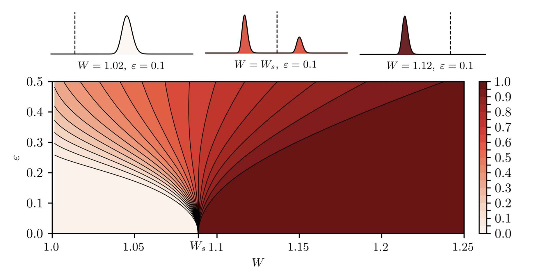
For practical applications it is useful to identify combinations of and that lead to confidence in whether the statistically steady state corresponds to forward or reverse flow. To this end, figure 6 plots isolines of the stationary probability , which is the probability of finding the system in the basin of attraction for reverse flow. Because the line demarcating forward and reverse flow (see, for example, figure 4) does not coincide with the local maxima of , reverse flow is theoretically possible even when the system is in the basin of attraction for forward flow. Consequently, probabilities corresponding to the likelihood of being in the basin of attraction for reverse flow underestimate (by an amount that diminishes with ) the probability of forward flow, i.e. .
The contours in figure 6 are characterised by a fan shaped region of uncertainty, in which the probability varies continuously between and , emanating from . On either side of this region of uncertainty are regions for which one can be close to certain that the system will eventually be in either the basin of attraction for forward or reverse flow. Plots such as (6) might provide a useful guide to engineers by identifying conditions for which it would be difficult or inappropriate to design for a single flow regime.
3.6 Kramer’s escape rate Kramer’s escape rate
The stationary densities discussed in the previous section are solutions to . How long one would have to wait in practice to see such solutions, however, would depend on the initial state of the system. For example, for small values of , wind strengths slightly larger than and an initial density in the region (forward flow), one might have to wait a long time for the density to be transported into (reverse flow) in the way that figure 6 suggests. The physical reason for such large time scales is that when the potential wells are both relatively deep, which, for small , means that a rare (infrequent) fluctuation in the system’s forcing is required to produce a transition between the two wells.
The remarks above can be made precise by considering a potential barrier , quantified as the difference between the local maxima and local minima associated with forward flow,
| (32) |
If the potential barrier is large relative to the diffusivity , the rate at which states ‘escape’ from (forward flow), quantified as the probability flux divided by the probability, can be approximated using Kramer’s escape rate formula [50]:
| (33) |
The associated timescale, , is plotted in figure 7 for the quadratic diffusion model . The figure shows that the time one can expect to wait to reach a stationary state decreases with respect to , which controls the height of the potential barrier, and increases with respect to , which quantifies the ‘destabilising’ noise. Since does not depend on , (33) suggests that the time that one would have to wait to reach a stationary density increases exponentially with respect to .

4 Numerical simulations Numerical simulations
To obtain individual realisations of the stochastic model, (8) can be integrated directly. Using the Heun method [38], which accounts for the drift induced by the Stratonovich interpretation of the noise without modification of the function ‘’ in (8), the discretised equations are
| (34) |
where , and
| (35) | ||||
| (36) |
are intermediate values of the drift and standard deviation based on the following estimate of the buoyancy at time :
| (37) |
The sample trajectories shown in figures 8 and 9 were obtained with for . A set of such realisations were obtained for a given value of to construct the histograms shown on the left-hand side of figures 8 and 9 (in this regard, note that each time series on the right-hand side is a single realisation). The stable fixed point for either forward flow ( shown in figure 8) or reverse flow ( shown in figure 9) was used as an initial condition for all realisations and statistically transient data for were not included in the construction of the histograms.
Figure 8 shows realisations for (cf. figure 5, for which the probability density would concentrate itself around the fixed point for forward flow in the limit ). For cases and , illustrated in the subplots and , respectively, the system’s trajectory crosses the potential barrier frequently, which leads to large variance and significant uncertainty regarding the direction of the ventilation. For in subplot , however, the system is likely to be found in forward flow and does not appear to transition between forward and reverse flow frequently. In contrast, figure 9 shows that when the system resides predominantly in reverse flow for the reasons described in §3. Whereas produces occasional excursions of the system into a state of forward flow, for and the flow is almost entirely in the reverse direction.
The histograms shown in figures 8 and 9 exhibit a reasonably good agreement with the analytical solution (23). The differences between the analytical solution and the histograms obtained from realisations of (8) in figure 8 illustrate the challenge of obtaining a sufficient number of samples for a system that undergoes infrequent transitions. Bearing in mind that the governing equations are nondimensional, figure 8 shows that one needs to collect data over extremely long durations/large ensembles in order to resolve the underlying density, which makes the availability of analytical solutions or approximations particularly attractive.
5 An Ornstein-Uhlenbeck (‘Langevin’) model An Ornstein-Uhlenbeck (‘Langevin’) model
As discussed in §2.2, the effects of fluctuations can be incorporated in several ways, which raises important questions concerning their physical origin and the correct interpretation of the deterministic equations to which they are added. In §2.2 fluctuations were included as a stochastic buoyancy flux; in this section, the stochastic evolution of the wind is specified as an additional equation. In general, such an equation could be adapted to produce a specific wind speed distribution from a given set of environmental conditions [22]. One particular, if somewhat idealised, approach is to represent fluctuations in the wind velocity that affect the bulk pressure difference ( in §2.1) as an Ornstein-Uhlenbeck process [18], which can account for temporal correlations. If the stochastic buoyancy flux from §2.1 is retained, the governing equations become
| (38) | ||||
| (39) |
where, following [18], corresponds to dimensionless fluctuations in the wind velocity, which is proportional to the square root of the resulting pressure difference:
| (40) |
The parameter determines the rate at which reverts to its mean value of zero and denotes uncorrelated increments of a zero-mean Gaussian process with time- and state-invariant standard deviation . One difference between (38)-(39) and the simpler version studied in §2.2 is that the stochastic forcing appears in the nonlinear drift term . A second difference is that the probability density corresponding to (38)-(39) is a joint density of two (rather than one) variables.
The Fokker-Planck equation for the joint density is
| (41) |
where
| (42) |
is the two-dimensional probability flux. Integrating (41) with respect to , gives an equation for that is satisfied by the stationary marginal density , which is the quantity of interest:
| (43) |
where, making use of the conditional density when ,
| (44) |
is the unknown conditional expectation of the the drift for a given value of . Unless the full equation (41) is solved, an assumption about the conditional expectation is required to make progress with (43).
If is sufficiently large, the modelled wind will evolve on a much faster time scale than the buoyancy and can be regarded as being in a state of quasi-equilibrium. Corresponding to such a separation of time scales is the assumption that derivatives with respect to of the conditional density are much larger than those with respect to . Consequently, when is substituted into (41) it is seen that can be approximated by a balance of terms involving only relatively large derivatives with respect to [31]:
| (45) |
which has the well-known solution [56]
| (46) |
In this particular case, for which does not feature in (39), in (46) corresponds to the stationary marginal density .
The subsequent use of obtained from (46) in (44) to account for the effect that the fast variable has on the evolution of the slow variable, while removing the former from the calculations, is known as ‘adiabatic elimination’ [57, 31]. With such an approximation, the drift term in (43) can be expressed as the gradient of the potential (5) that is convolved with the marginal density of the fast variable:
| (47) |
where, noting that from (46) does not depend on ,
| (48) |
Figure 10 displays contours of along with ‘equilibrium’ paths corresponding to its local extrema. Sufficiently large wind fluctuations (small ) modify the original potential (see cf. figure 2) via the convolution (48) by removing the metastable equilibrium corresponding to forward flow at large wind strengths . When , the potential is convex and has a unique minimum corresponding to forward or reverse flow for small or large values of , respectively. It is in this way that the nonlinear effects of fluctuations in the wind strength in (38) modify the underlying structure of the equation, regardless of noise in the buoyancy flux that can be included separately in (38) with a particular parameterisation for .
As illustrated in figure 11, which shows equilibria of the potential surface as a function of both and , the cusp point of the potential, above which a second local minimum in emerges, is . The relevance of this number to practical applications will be discussed at the end of the next section.

6 Application Application
Although it is convenient to use nondimensionalised equations (4), it is useful to consider how the results relate to the dimensional parameters that might be encountered in practice. For the quadratic diffusion model applied to the buoyancy flux in §3.2, characterises the effects of uni- or bi-directional fluctuations in the flow through an opening. While it is therefore difficult to relate wind speed statistics to in a precise way without a model developed from first principles, it is instructive to consider the dimensional version of the equations (cf. (1)), for which care is needed in deducing the correct nondimensionalisation of :
| (49) |
In (49) the Wiener process has dimensions corresponding to the square root of time and is the dimensional version of (18). Therefore, noting that each term in (49) has dimensions , where the dimensions of length and time are denoted as and , respectively, implies that .
If corresponds to a velocity scale that characterises fluctuations in the buoyancy flux through the opening, then it is reasonable to express in terms of and the opening area , such that on dimensional grounds; hence, nondimensionalising and in (49) using (3) and (3), respectively,
| (50) |
which, when compared with (8), shows that
| (51) |
If the strength of the fluctuations is related to the wind-induced pressure difference by , where is a dimensionless number that can account for orientation and the statistical properties of the wind, then (2) and (3) can be used to express in terms of , such that (51) becomes
| (52) |
Equation (52) is useful because it provides an algebraic relationship between and for which the prefactor is determined by the geometric properties of the room/building. For a typical meeting room of cross-sectional area , height and effective opening area , (52) implies that, for (corresponding to , which is equivalent to approximately of heat), . More generally, figure 12 displays the stationary probability density using (52) to relate and for , and the geometric parameters stated above. The central message conveyed by figure 12 is that, for realistic geometric parameters and wind fluctuations that are of the same order of magnitude as the strength of an opposing wind, sustained buoyancy-driven flow opposing the wind direction is extremely unlikely for wind strengths that exceed the statistically critical value . However, for statistically transient states arising, for example, from temporal changes in either or , characterising the behaviour of the system probabilistically is more challenging.
The time scale associated with the dimensional parameters discussed above is
| (53) |
Multiplying the nondimensional time scale from figure 7 by (53) along the dashed line corresponding to (52) shows that the time one would have to wait for such a system to settle into the stationary state shown in figure 12, having started in forward flow, could be comparable to the durations for which such a room is likely to be used (i.e. in the order of one hour). Considerations of the transient evolution of the probability density would therefore play an important role in such applications. While relatively small fluctuations correspond to certainty regarding the eventual state of the flow, they correspond to uncertainty in producing a longer transient period than relatively large fluctuations. However, for relatively large base wind strengths (e.g. ), it is likely that the system would settle into reverse flow in a matter of minutes.
For the Ornstein-Uhlenbeck process discussed in §5, the random variable corresponds to fluctuations in the wind speed divided by the base velocity scale used to define in (3). The statistics reported in a recent study on stochastic models for wind[22, 18] suggest that plausible values of in (46) lie between and and therefore encompass the bifurcation illustrated in figure 11. Relatively small values of within this range (relatively long, large gusts of wind) will lead to reverse flow for large base wind strengths, whereas relatively large values of (relatively short, small gusts of wind) do not necessarily rule out the possibility of forward flow at large base wind strengths.
7 Conclusions Conclusions
This work has described stochastic models for natural ventilation driven by opposing wind and buoyancy. The results expose several properties concerning the system’s predictability and stability for the first time and highlight challenges associated with the incorporation of stochastic effects into existing deterministic models for ventilation.
In the absence of rigorous justification for a particular form of stochastic forcing from either theory or experiments, the models chosen for this study were simple and of general applicability. In §2.2 a stochastic buoyancy flux was added to the deterministic evolution of buoyancy in the form of a Stratonovich integral of a Wiener process (8) as the limit of a stochastic process with relatively short autocorrelation time. In general, the approach can account for fluctuations of the buoyancy flux that depend on the system’s state and the base wind strength . The evolution of the resulting probability density is determined by a Fokker-Planck equation which accounts for the stabilising effects of the underlying potential and the destabilising effects of noise. An analytically-defined Boltzmann-like distribution describes the corresponding stationary density. In §5 the wind itself was modelled as an Ornstein-Uhlenbeck process at the expense of introducing an additional dimension, which was subsequently approximated using adiabatic elimination.
Although the deterministic system for this problem admits multiple steady states, for sufficiently large opposing wind strengths and small amounts of noise, the system’s stationary state is unlikely to be found in the metastable region associated with forward flow. As the wind strength increases, fluctuations in the buoyancy flux are, with increasing likelihood, able to overcome the relatively small potential barrier separating forward and reverse flow. Another reason is that when the wind itself is modelled as a stochastic process (see §5), fluctuations in the wind convolve with the nonlinear function describing the system’s underlying potential, which can lead to the removal of the metastable equilibrium altogether, as shown in figure 10. In these respects, the state of the stochastic system, which accounts for disturbances that are likely to be present in practical applications, is easier to ‘determine’ in a design context than it would be for the idealised ‘deterministic’ system. Although the particularities of such results depend on the choice of stochastic model, their qualitative properties are generic and expected to be found in a broad range of possible stochastic models.
An important caveat to the conclusions above is that certainty in the eventual state of the system goes hand in hand with uncertainty associated with an increase in the duration of the transient evolution of the probability density. It is therefore difficult to be prescriptive about whether the system is likely to be in a particular state without careful consideration of the base wind strength and relative size of the fluctuations. Base wind strengths that are close to critical are the most difficult in this regard, because they are associated with bimodal probability densities with transients of the longest duration.
A preeminent challenge to the future incorporation of stochastic effects in existing deterministic models of ventilation is finding physically faithful interpretations and representations of fluctuations, and reconciling them with the established deterministic part of such models. In bulk models of turbulence it is not always clear whether the established deterministic equations represent the limit of a system with zero external noise or as the macroscopic average of a system with finite (internal) noise. The former interpretation is somewhat easier to approach theoretically and, if regarded as the limit of a process with relatively short autocorrelation times, is consistent with our use of the Stratonovich integral in (8) [45].
When systems involve internal noise (which is arguably always the case where turbulence is concerned) the situation is more complicated because the fluctuations can’t be removed. In that case it would be necessary to return to fundamentals and develop a master equation for the system’s probability density from first principles, rather than trying to ascribe meaning to an otherwise ill-defined deterministic equation (4) from a Langevin perspective [45]. With a suitable master equation determining every aspect of the system’s evolution, the frequently debated ‘choice’ between Itô or Stratonovich integration, would be irrelevant because the corresponding Langevin equation for either approach would be defined to ensure consistency with the underlying master equation.
Hopefully the considerations above will motivate dedicated experiments and direct simulations of turbulence to underpin a rigorous formulation of the required stochastic equations, which are likely to play an important role in future applications.
8 Acknowledgements Acknowledgements
This work was supported by the Engineering and Physical Sciences Research Council [grant number EP/V033883/1] as part of the [D∗]stratify project.
References
- [1] Linden PF. 1999 The fluid mechanics of natural ventilation. Annual Review of Fluid Mechanics 31, 201–238. (10.1146/annurev.fluid.31.1.201)
- [2] Hunt GR, Linden PF. 2005 Displacement and mixing ventilation driven by opposing wind and buoyancy. Journal of Fluid Mechanics 527, 27–55.
- [3] Hunt GR, Linden PF. 1999 The fluid mechanics of natural ventilation–displacement ventilation by buoyancy-driven flows assisted by wind. Building and Environment 34, 707 – 720.
- [4] Ouf MM, O’Brien W, Gunay B. 2019 On quantifying building performance adaptability to variable occupancy. Building and Environment 155, 257–267. (https://doi.org/10.1016/j.buildenv.2019.03.048)
- [5] Hong T, Taylor-Lange SC, D’Oca S, Yan D, Corgnati SP. 2016 Advances in research and applications of energy-related occupant behavior in buildings. Energy and Buildings 116, 694–702. (https://doi.org/10.1016/j.enbuild.2015.11.052)
- [6] Delzendeh E, Wu S, Lee A, Zhou Y. 2017 The impact of occupants’ behaviours on building energy analysis: A research review. Renewable and Sustainable Energy Reviews 80, 1061–1071. (https://doi.org/10.1016/j.rser.2017.05.264)
- [7] Sun K, Hong T. 2017 A framework for quantifying the impact of occupant behavior on energy savings of energy conservation measures. Energy and Buildings 146, 383–396. (https://doi.org/10.1016/j.enbuild.2017.04.065)
- [8] Laaroussi Y, Bahrar M, Elmankibi M, Draoui A, Si-Larbi A. 2019 Occupant behaviour: a major issue for building energy performance. In IOP Conference Series: Materials Science and Engineering vol. 609 p. 072050. IOP Publishing. (10.1088/1757-899X/609/7/072050)
- [9] Boettcher F, Renner C, Waldl HP, Peinke J. 2003 On the statistics of wind gusts. Boundary-Layer Meteorology 108, 163–173.
- [10] Coceal O, Thomas TG, Castro IP, Belcher SE. 2006 Mean flow and turbulence statistics over groups of urban-like cubical obstacles. Boundary-Layer Meteorology 121, 491–519.
- [11] Efthimiou G, Hertwig D, Andronopoulos S, Bartzis J, Coceal O. 2017 A statistical model for the prediction of wind-speed probabilities in the atmospheric surface layer. Boundary-Layer Meteorology 163, 179–201.
- [12] Burridge HC, Bhagat RK, Stettler MEJ, Kumar P, De Mel I, Demis P, Hart A, Johnson-Llambias Y, King MF, Klymenko O, McMillan A, Morawiecki P, Pennington T, Short M, Sykes D, Trinh PH, Wilson SK, Wong C, Wragg H, Davies Wykes MS, Iddon C, Woods AW, Mingotti N, Bhamidipati N, Woodward H, Beggs C, Davies H, Fitzgerald S, Pain C, Linden PF. 2021 The ventilation of buildings and other mitigating measures for COVID-19: a focus on wintertime. Proceedings of the Royal Society A: Mathematical, Physical and Engineering Sciences 477, 20200855. (10.1098/rspa.2020.0855)
- [13] Bhagat RK, Davies Wykes MS, Dalziel SB, Linden PF. 2020 Effects of ventilation on the indoor spread of COVID-19. Journal of Fluid Mechanics 903, F1. (10.1017/jfm.2020.720)
- [14] Batchelor GK. 1954 Heat convection and buoyancy effects in fluids. Quarterly Journal of the Royal Meteorological Society 80, 339–358.
- [15] Linden PF, Lane-Serff GF, Smeed DA. 1990 Emptying filling boxes: the fluid mechanics of natural ventilation. Journal of Fluid Mechanics 212, 309–335.
- [16] Baines WD, Turner JS. 1969 Turbulent buoyant convection from a source in a confined region. Journal of Fluid Mechanics 37, 51–80. (10.1017/S0022112069000413)
- [17] Karava P, Stathopoulos T, Athienitis A. 2004 Wind Driven Flow through Openings – A Review of Discharge Coefficients. International Journal of Ventilation 3, 255–266. (10.1080/14733315.2004.11683920)
- [18] Vesipa R, Ridolfi L, Salizzoni P. 2023 Wind fluctuations affect the mean behaviour of naturally ventilated systems. Building and Environment 229, 109928. (https://doi.org/10.1016/j.buildenv.2022.109928)
- [19] Leprince J, Madsen H, Miller C, Real JP, van der Vlist R, Basu K, Zeiler W. 2022 Fifty shades of grey: Automated stochastic model identification of building heat dynamics. Energy and Buildings 266, 112095. (https://doi.org/10.1016/j.enbuild.2022.112095)
- [20] Wolf S, Cali D, Krogstie J, Madsen H. 2019 Carbon dioxide-based occupancy estimation using stochastic differential equations. Applied Energy 236, 32–41. (https://doi.org/10.1016/j.apenergy.2018.11.078)
- [21] Macarulla M, Casals M, Forcada N, Gangolells M, Giretti A. 2018 Estimation of a room ventilation air change rate using a stochastic grey-box modelling approach. Measurement 124, 539–548. (https://doi.org/10.1016/j.measurement.2018.04.029)
- [22] Ma J, Fouladirad M, Grall A. 2018 Flexible wind speed generation model: Markov chain with an embedded diffusion process. Energy 164, 316–328. (https://doi.org/10.1016/j.energy.2018.08.212)
- [23] Palmer T, Williams P. 2008 Introduction. Stochastic physics and climate modelling. Philosophical Transactions of the Royal Society A: Mathematical, Physical and Engineering Sciences 366, 2419–2425. (10.1098/rsta.2008.0059)
- [24] Fontanini A, Vaidya U, Ganapathysubramanian B. 2013 A stochastic approach to modeling the dynamics of natural ventilation systems. Energy and Buildings 63, 87–97. (https://doi.org/10.1016/j.enbuild.2013.03.053)
- [25] Coomaraswamy I, Caulfield C. 2011 Time-dependent ventilation flows driven by opposing wind and buoyancy. Journal of fluid mechanics 672, 33–59.
- [26] Bellman R, Kalaba R. 1959 A mathematical theory of adaptive control processes. Proceedings of the National Academy of Sciences 45, 1288–1290.
- [27] Van Kampen N. 2011 Stochastic Processes in Physics and Chemistry. North-Holland Personal Library. Elsevier Science.
- [28] Li Y, Delsante A. 2001 Natural ventilation induced by combined wind and thermal forces. Building and Environment 36, 59–71.
- [29] Chenvidyakarn T, Woods A. 2005 Multiple steady states in stack ventilation. Building and Environment 40, 399 – 410. (https://doi.org/10.1016/j.buildenv.2004.06.020)
- [30] Strogatz S. 1994 Nonlinear Dynamics and Chaos: With Applications to Physics, Biology, Chemistry, and Engineering. Addison-Wesley.
- [31] Haken H. 1983 Synergetics: An Introduction. Springer Series in Synergetics. Springer-Verlag.
- [32] Yuan J, Glicksman LR. 2008 Multiple steady states in combined buoyancy and wind driven natural ventilation: The conditions for multiple solutions and the critical point for initial conditions. Building and Environment 43, 62–69. (https://doi.org/10.1016/j.buildenv.2006.11.035)
- [33] Lishman B, Woods AW. 2009 On transitions in natural ventilation flow driven by changes in the wind. Building and Environment 44, 666–673.
- [34] Craske J, Hughes G. 2019 On the robustness of emptying filling boxes to sudden changes in the wind. Journal of Fluid Mechanics 868, R3. (10.1017/jfm.2019.199)
- [35] Grafke T, Vanden-Eijnden E. 2017 Non-equilibrium transitions in multiscale systems with a bifurcating slow manifold. Journal of Statistical Mechanics: Theory and Experiment 2017, 093208. (10.1088/1742-5468/aa85cb)
- [36] Meunier C, Verga A. 1988 Noise and bifurcations. Journal of Statistical Physics 50, 345–375.
- [37] Kuehn C. 2011 A mathematical framework for critical transitions: Bifurcations, fast–slow systems and stochastic dynamics. Physica D: Nonlinear Phenomena 240, 1020–1035. (https://doi.org/10.1016/j.physd.2011.02.012)
- [38] Burrage K, Burrage PM, Tian T. 2004 Numerical methods for strong solutions of stochastic differential equations: an overview. Proceedings of the Royal Society of London. Series A: Mathematical, Physical and Engineering Sciences 460, 373–402. (10.1098/rspa.2003.1247)
- [39] Schenk-Hoppé KR. 1996 Bifurcation scenarios of the noisy Duffing-van der Pol oscillator. Nonlinear Dynamics 11, 255–274.
- [40] Mendez A, Farazmand M. 2021 Investigating climate tipping points under various emission reduction and carbon capture scenarios with a stochastic climate model. Proceedings of the Royal Society A: Mathematical, Physical and Engineering Sciences 477, 20210697. (10.1098/rspa.2021.0697)
- [41] Namachchivaya NS. 1990 Stochastic bifurcation. Applied Mathematics and Computation 38, 101–159.
- [42] Kramers H. 1940 Brownian motion in a field of force and the diffusion model of chemical reactions. Physica 7, 284–304. (https://doi.org/10.1016/S0031-8914(40)90098-2)
- [43] Virgin LN, Plaut RH, Cheng CC. 1992 Prediction of escape from a potential well under harmonic excitation. International Journal of Non-Linear Mechanics 27, 357–365. (https://doi.org/10.1016/0020-7462(92)90005-R)
- [44] Gladstone C, Woods AW. 2001 On buoyancy-driven natural ventilation of a room with a heated floor. Journal of Fluid Mechanics 441, 293–314. (10.1017/S0022112001004876)
- [45] van Kampen NG. 1981 Itô versus Stratonovich. Journal of Statistical Physics 24, 175–187. (10.1007/BF01007642)
- [46] Resnick S. 1992 Adventures in Stochastic Processes. Adventures in Stochastic Processes. Birkhäuser Boston.
- [47] Moon W, Wettlaufer JS. 2014 On the interpretation of Stratonovich calculus. New Journal of Physics 16, 055017. (10.1088/1367-2630/16/5/055017)
- [48] Doob JL. 1942 The Brownian Movement and Stochastic Equations. Annals of Mathematics 43, 351–369.
- [49] Uhlenbeck GE, Ornstein LS. 1930 On the Theory of the Brownian Motion. Phys. Rev. 36, 823–841. (10.1103/PhysRev.36.823)
- [50] Risken H, Frank T. 1996 The Fokker-Planck Equation: Methods of Solution and Applications. Springer Series in Synergetics. Springer-Verlag.
- [51] Einstein AB On the movement of small particles suspended in a stationary liquid demanded by the molecular-kinetic theory of heart. Annalen der Physik 17, 549–560.
- [52] Langevin P. 1908 Sur la théorie du mouvement brownien. Compt. Rendus 146, 530–533.
- [53] Gillespie DT. 1996 Exact numerical simulation of the Ornstein-Uhlenbeck process and its integral. Phys. Rev. E 54, 2084–2091. (10.1103/PhysRevE.54.2084)
- [54] Lemons DS, Gythiel A. 1997 Paul Langevin’s 1908 paper “On the Theory of Brownian Motion” [“Sur la théorie du mouvement brownien,” C. R. Acad. Sci. (Paris) 146, 530–533 (1908)]. American Journal of Physics 65, 1079–1081. (10.1119/1.18725)
- [55] Landau L, Lifshitz E. 2013 Statistical Physics: Volume 5. Elsevier Science.
- [56] Gardiner C. 1985 Handbook of Stochastic Methods: For Physics, Chemistry and the Natural Sciences. Lecture Notes in Mathematics. Springer-Verlag.
- [57] Theiss W, Titulaer U. 1985 The systematic adiabatic elimination of fast variables from a many-dimensional Fokker-Planck equation. Physica A: Statistical Mechanics and its Applications 130, 123–142. (https://doi.org/10.1016/0378-4371(85)90100-1)