1INTRODUCTION

Bayesian Optimization over High-Dimensional Combinatorial Spaces
via Dictionary-based Embeddings

Aryan Deshwal Sebastian Ament Maximilian Balandat Eytan Bakshy Washington State University Meta Meta Meta

Janardhan Rao Doppa David Eriksson Washington State University Meta

Abstract

We consider the problem of optimizing expensive black-box functions over high-dimensional combinatorial spaces which arises in many science, engineering, and ML applications. We use Bayesian Optimization (BO) and propose a novel surrogate modeling approach for efficiently handling a large number of binary and categorical parameters. The key idea is to select a number of discrete structures from the input space (the dictionary) and use them to define an ordinal embedding for high-dimensional combinatorial structures. This allows us to use existing Gaussian process models for continuous spaces. We develop a principled approach based on binary wavelets to construct dictionaries for binary spaces, and propose a randomized construction method that generalizes to categorical spaces. We provide theoretical justification to support the effectiveness of the dictionary-based embeddings. Our experiments on diverse real-world benchmarks demonstrate the effectiveness of our proposed surrogate modeling approach over state-of-the-art BO methods.

1 INTRODUCTION

Many real-world applications require building probabilistic models over high-dimensional discrete and mixed (involving both discrete and continuous parameters) input spaces using limited training data. These models need to make accurate predictions and quantify the uncertainty for unknown inputs. Some examples include calibration of environment models, feature selection for automated machine learning (AutoML) where the inclusion/exclusion of a given feature can be represented by a binary parameter, and microbiome analysis where the inclusion/exclusion of a microbial species is a binary parameter and environmental variables correspond to continuous parameters.

Gaussian processes (GPs) (Rasmussen 2004) are well-suited for this setting. GPs are also commonly used as surrogate models for sample-efficient optimization of expensive black-box functions over both continuous and discrete/mixed spaces (Frazier 2018). For instance, in microbiome design optimization we need to perform expensive wet lab experiments to evaluate each mixed configuration in the form of a subset of candidate microbes and environmental conditions (Clark et al. 2021). Other example applications include feature selection for ML models Guyon and Elisseeff 2003, tuning flags of a compiler to optimize efficiency Hellsten et al. 2022, and tuning database configurations Zhang et al. 2021. The key challenge in using GPs for combinatorial spaces is to define an appropriate kernel to capture the similarity between input pairs.

This paper proposes a novel Hamming embedding via dictionaries (HED). This embedding allows us to leverage popular GP kernels with automatic relevance determination (ARD) for modeling high-dimensional combinatorial inputs. Our method naturally extends to mixed inputs with both continuous and discrete variables by using a product kernel. The key idea in our modeling approach is to select a fixed number of candidate structures from the input space, referred to as a dictionary, and to define an embedding for the input space using the Hamming distance of the inputs to elements in the dictionary. The effectiveness of this approach critically depends on the choice of the dictionary. Our theoretical analysis shows that the regret bound for GP bandits (Srinivas et al. 2010) trained on the HED is a function of the cardinality of the embedded search space, which in turn is a function of a notion of orthogonality of the dictionary. We observe that constructing dictionaries that initially limit the collapse of the search space cardinality exhibit a high degree of modeling flexibility, which leads to a data-driven compression of the search space and empirically faster convergence. Motivated by these theoretical insights, we propose two methods to construct dictionaries: 1) sub-sampled binary wavelets (Swanson and Tewfik 1996), which optimize the orthogonality measure in power-of-two dimensions, and 2) a randomized method that generalizes to categorical inputs and allows us to design dictionaries of any size.

To evaluate the effectiveness of dictionary-based embeddings, we consider several expensive black-box optimization problems within the framework of Bayesian optimization (BO). Applying BO to combinatorial spaces comes with unique challenges (Doppa 2021) since commonly used surrogate models often do not work well in this setting and because we cannot rely on gradient-based methods to optimize the utility function. Examples of surrogate models that have been applied in combinatorial spaces include GPs with diffusion kernels (Oh et al. 2019), GPs with isotropic kernels (Wan et al. 2021), linear models (Baptista and Poloczek 2018), and random forests (Hutter et al. 2011; Deshwal et al. 2020). When the dictionary-based embeddings are used for Bayesian optimization, we refer to this as BO with Dictionaries (BODi). Our comprehensive experimental evaluation on BO benchmarks demonstrate the efficacy of BODi over state-of-the-art methods and provide empirical evidence that BODi’s strong performance is due to dictionary-based surrogate model.

The key contribution of this paper is the development and evaluation of our dictionary-based modeling approach. Our specific contributions include:

1.

A dictionary-based embedding that substantially improves the quality of GP models in high-dimensional combinatorial and mixed input spaces.
2.

Two methods of constructing the dictionary: 1) via binary wavelets, and 2) a randomized construction method that generalizes to arbitrary dimensions and categorical variables.
3.

A theoretical analysis of our approach shows that it compresses the cardinality of the input space under certain conditions, and if ARD is used, in a data-dependent fashion.
4.

The compressed cardinality leads to improved regret bounds for GP Bandits with binary inputs.
5.

A comprehensive experimental evaluation on diverse set of combinatorial and mixed BO benchmarks demonstrate the effectiveness of BODi. The source code is available at https://github.com/aryandeshwal/BODi.

2 BACKGROUND

Combinatorial and mixed spaces.

Let $\mathcal{Z}$ be a combinatorial space where each element $\mathbb{z}\in\mathcal{Z}$ is a discrete structure. We assume $\mathbb{z}\in\mathcal{Z}$ can be represented using $d$ discrete variables $v_{1},v_{2},\cdots,v_{d}$ where each variable $v_{i}$ takes values from a finite candidate set $C(v_{i})$ . Each variable $v_{i}$ takes $\tau_{i}\geq 2$ possible values and the cardinality of the space is $|\mathcal{Z}|=\prod_{i=1}^{d}\tau_{i}$ . In particular, for binary spaces, $C(v_{i})=\{0,\,1\}$ for all $v_{i}$ and $|\mathcal{Z}|=2^{d}$ . If $\mathcal{X}$ is a space of continuous parameters, we call $\mathcal{X}\times\mathcal{Z}$ a mixed space.

Problem definition.

We are given a high-dimensional combinatorial space $\mathcal{Z}$ , i.e., the number of discrete variables $d$ is large. We assume we are optimizing a black-box objective function $f:\mathcal{Z}\mapsto\mathbb{R}$ , which we can evaluate on each structure $\mathbb{z}\in\mathcal{Z}$ . For example, in feature selection for Auto ML tasks, $\mathbb{z}$ is a binary structure corresponding to a subset of features and $f(\mathbb{z})$ is the performance of a trained ML model using the selected features. Our goal is to find a structure $\mathbb{z}\in\mathcal{Z}$ that approximately optimizes $f$ given a small number of function evaluations.

Bayesian optimization.

BO methods build a probabilistic surrogate model $\mathcal{M}$ , often a GP, from the training data of past function evaluations and intelligently select the sequence of inputs for evaluation in a sample-efficient manner. The selection of inputs is performed by maximizing an acquisition function $\alpha$ that operates on the posterior distribution provided by the surrogate model. One of the key challenges in using BO for high-dimensional combinatorial spaces is to build accurate surrogate models, which is the central focus of our work.

Gaussian processes.

GPs are non-parametric probabilistic models that are popular due to their flexibility and excellent uncertainty quantification. A GP is specified by a mean function and a covariance function or kernel $k:\mathbb{R}\times\mathbb{R}\to\mathbb{R}$ (Rasmussen 2004). A common choice is the RBF or squared exponential kernel, which is given by

k(\mathbf{x},\mathbf{y})=s^{2}\exp\Bigl\{-\tfrac{1}{2}\sum_{i}(x_{i}-y_{i})^{2}/\ell_{i}^{2}\Bigr\}

where $\ell_{i}$ for $i=1,\cdots,D$ are the lengthscales that allow for automatic relevance determination (ARD) and $s^{2}$ is the signal variance.

3 RELATED WORK

Discrete and mixed spaces.

In recent years, BO over discrete and mixed spaces has received considerable attention due to its wide applicability to science, engineering, AutoML, and other domains. A variety of surrogate models have been proposed for the low-dimensional setting, but those are typically not effective for high-dimensional spaces, as we demonstrate in our experiments.

BOCS (Baptista and Poloczek 2018) targets binary spaces and employs a second-order Bayesian linear regression surrogate model, which exhibits poor scaling in the input dimension and may not support applications where the underlying black-box function requires a more complex model. Prior work also considers different instantiations of GP models. COMBO (Oh et al. 2019; Deshwal et al. 2021a) employs GPs with discrete diffusion kernels over a combinatorial graph representation of the input space. Recently, Kim et al. 2022 proposed an approach for combinatorial spaces based on continuous embeddings. Their approach differs from ours in that they employ a uniformly random injective mapping and need to reconstruct the discrete input after optimizing the acquisition function in the embedded space. There is also work on using deep generative models to create a latent space and apply continuous BO methods (often referred to as “latent space BO”): Gómez-Bombarelli et al. 2018; Tripp et al. 2020; Eissman et al. 2018; Kajino 2019; Notin et al. 2021; Deshwal and Doppa 2021; Maus et al. 2022. In contrast, our dictionary-based embeddings are computationally efficient and leverage the inherent structure in the combinatorial space. It is a fruitful direction to explore ways to synergistically combine the benefits of latent space and dictionary-based embeddings.

There is also prior work on approaches for constructing kernels over mixed spaces with both discrete and continuous variables (Ru et al. 2020; Oh et al. 2021; Deshwal et al. 2021b). Garrido-Merchán and Hernández-Lobato 2020 round the input variables before passing it to a GP with a canonical kernel. Tree-Parzen Estimators (TPEs) (Bergstra et al. 2011) are applicable to mixed spaces and consider density estimation in the input space which is potentially challenging in high-dimensional settings. SMAC (Hutter et al. 2011) employs a random forest surrogate model.

High-dimensional continuous spaces.

There is a large body of work on BO over high-dimensional continuous spaces which can be classified into the following categories: (1) Low-dimensional structure, which may be random embeddings (Wang et al. 2016; Letham et al. 2020; Papenmeier et al. 2022), hashing-based approaches (Nayebi et al. 2019), sparsity-inducing priors (Eriksson and Jankowiak 2021), or learned embeddings (Garnett et al. 2013). (2) Additive structure (Kandasamy et al. 2015; Gardner et al. 2017), which assumes that the high-dimensional black-box function decomposes into a sum of low-dimensional functions. (3) Methods that avoid selecting highly uncertain boundary points. Eriksson et al. 2019 use local trust regions centered around the best solutions and these trust regions are resized based on progress. Kirschner et al. 2019 optimize the acquisition function along one-dimensional lines, and Oh et al. 2018 use a cylindrical kernel to focus on the interior of the domain.

Refer to caption — Figure 1: High-level overview of our BODi algorithm for binary spaces. The dictionary ${\mathbb{A}}$ contains $m$ discrete structures from the combinatorial space $\mathcal{Z}$ . Each high-dimensional binary structure $\mathbf{z}\in\mathcal{Z}$ (denoted by black and white squares) is embedded into a low-dimensional embedding ${\bm{\phi}}_{\mathbb{A}}(\mathbf{z})\in\mathbb{R}^{m}$ (denoted by colored squares). We learn a GP surrogate model over the embedded space and perform acquisition function optimization in the original combinatorial space $\mathcal{Z}$ to select the next structure $\mathbf{z}_{next}$ for function evaluation in each BO iteration.

These methods, however, are specific to continuous spaces and there is little work on studying the challenges of high-dimensional combinatorial and mixed search spaces which arise in many real-world applications. One exception is the recently proposed CASMOPOLITAN method (Wan et al. 2021), which uses adaptive trust regions from continuous spaces (Eriksson et al. 2019) by replacing the standard Euclidean distance with Hamming distance for discrete (sub)spaces. Our proposed BODi algorithm and the associated dictionary-based kernel improve over CASMOPOLITAN in the high-dimensional setting.

4 DICTIONARY EMBEDDINGS

In this section, we introduce the idea of a Hamming embedding via dictionaries (HED), a novel embedding for binary and categorical inputs that embeds the inputs into an ordinal feature space. In particular, we employ a GP over the embedding ${\bm{\phi}}_{\mathbb{A}}(\mathbb{z})$ based on a dictionary ${\mathbb{A}}$ containing $m$ discrete $d$ -dimensional elements from the input space $\mathcal{Z}$ . The embedding ${\bm{\phi}}_{\mathbb{A}}(\mathbb{z})$ of size $m$ is obtained by computing the Hamming distance $h$ between $\mathbb{z}\in\mathcal{Z}$ and each element of the dictionary $\mathbb{{\mathbb{a}}}_{i}\in{\mathbb{A}}$ . That is,

[{\bm{\phi}}_{\mathbb{A}}(\mathbf{z})]_{i}=h({\mathbb{a}}_{i},\mathbf{z}).

HED has several advantages. First, it allows us to transform the challenging task of building models over high-dimensional discrete spaces into an application of GPs to the well-understood continuous space settings. This subsequently allows us to perform inference of lengthscales associated with the embedding representations, in contrast to the original categorical space where one lengthscale models the effect of a single category change. Further, the efficient inference of lengthscales due to the embedding enables Automatic Relevance Determination (ARD) to prune away redundant dimensions effectively, which we prove reduces the cardinality of the input space. We show theoretically that this improves the sample-efficiency of GP bandits (UCB), commonly used for BO, and produces state-of-the-art results for BO on high-dimensional combinatorial spaces. Further, while the core kernel is for binary spaces, it can easily be extended to mixed spaces with both continuous and discrete parameters by using a product kernel.

(a) Naïve random dictionary

(b) Binary wavelet dictionary

Figure 2: Mean predictions and associated

95

% predictive intervals on a MaxSAT problem with 60 binary variables (see details in Sec. 7), comparing naïve random (left) and binary wavelet (right) dictionaries, using

50

training points and predicting on

50

test points.

Dictionary construction procedure.

The effectiveness of HED depends on the dictionary construction. A naïve approach is to simply pick elements from the binary space uniformly at random. However, this naïve approach turns out to exhibit poor predictive or BO performance on the test problems considered in this work. For example, Fig. 2a illustrates the poor predictive performance of a GP using a dictionary kernel with a uniformly random binary dictionary on a MaxSAT test problem with $60$ binary variables.

Another idea is to use deterministic dictionary construction methods, such as multi-resolution wavelets (Mallat 1989), effective and well-known tools for studying real-valued signals at different scales by applying a set of orthogonal transforms to the data. In the context of binary spaces, binary wavelet transforms (Swanson and Tewfik 1996) are highly related to the well-known orthogonal Hadamard matrices, and are applied in signal processing, spectroscopy, and cryptography (Hedayat and Wallis 1978; Horadam 2012). In contrast to the naïve random dictionary, sub-sampled binary wavelet dictionaries lead to great predictive performance on the same MaxSAT problem, as shown in Fig. 2b.

While binary wavelets constitute powerful dictionary designs for predictive and optimization problems in binary search spaces (for associated optimization results, see Fig. 7), their construction for non powers-of-two is non-trivial, and even their existence for arbitrary dimensions is an open problem (Hadamard 1893; Baumert et al. 1962; Djoković et al. 2014). For this reason, we sub-sample the columns of the power-of-two dimensional binary wavelets for our experiments in non-power-of-two dimensions, see App. C for details.

To alleviate the difficulties around the general construction of binary wavelets, and to generalize our method to categorical spaces, we propose a randomized procedure that produces dictionary rows with a large range of sparsity levels. We refer to this randomized procedure as “diverse random.”

Algorithm 1 provides pseudo-code for constructing diverse random dictionaries defined over binary input spaces $\{0,1\}^{d}$ . The key principle of this construction procedure is to diversify the dictionary rows by generating binary vectors determined by different bias parameters ( $\theta$ ) of the Bernoulli distribution, unlike the naïve random where $\theta$ is always $1/2$ . Therefore, the rows of the naïve random dictionaries tend to have close to $d/2$ non-zeros as $d$ grows, whereas the diverse random dictionaries exhibit a large range of sparsity levels due to varying $\theta$ . This algorithm can easily be generalized to inputs with categorical variables of different sizes, see App. G for details. To summarize, the diverse random dictionaries can be constructed for arbitrary dimensions, extends naturally to categorical inputs, and as we will show later exhibits strong optimization performance on a wide range of benchmark problems.

Algorithm 1 Dictionary design for binary input space

\{0,1\}^{d}

with diversely sparse rows

requires: dictionary size $m$

1: Dictionary

{\mathbb{A}}\leftarrow

empty

2: for

i

1,2,\ldots,m

{\mathbb{a}}_{i}\leftarrow

empty

4: Sample Bernoulli parameter

\theta\sim\text{Uniform}(0,1)

5: for

j

1,2,\ldots,d

6: Sample binary number

a\sim\text{Bernoulli}(\theta)

{\mathbb{a}}_{i}\leftarrow{\mathbb{a}}_{i}\cup a

8: end for

9: Add

{\mathbb{a}}_{i}

to dictionary:

{\mathbb{A}}\leftarrow{\mathbb{A}}\cup{\mathbb{a}}_{i}

10: end for

11: return the dictionary

{\mathbb{A}}

of size

m\times d

Representation of mixed input spaces.

We have focused on a purely combinatorial input spaces $\mathcal{Z}$ , but can naturally extend our approach to mixed search spaces consisting of both discrete and continuous parameters. In this setting, we aim to model an input space $\mathcal{X}\times\mathcal{Z}$ where $\mathcal{X}$ is the domain of the continuous parameters. To extend our approach to this mixed inputs setting, we use a product kernel leveraging the HED embedding for discrete parameters and a standard, e.g., Matérn- $5/2$ kernel with ARD for the continuous parameters.

5 BODi: BAYESIAN OPTIMIZATION WITH DICTIONARY EMBEDDINGS

Our proposed BODi method is a straightforward instantiation of the generic BO framework. We use a GP with a standard Matérn- $5/2$ kernel with ARD on the HED embedding as the surrogate model, and we adopt the commonly used Expected Improvement (EI) acquisition function for single-objective problems. In our setting, EI takes as inputs the surrogate model $\mathcal{M}$ and the embedding ${\bm{\phi}}_{\mathbb{A}}(\mathbb{z})$ to score the utility of evaluating the structure $\mathbb{z}\in\mathcal{Z}$ . In order to optimize the acquisition function over the discrete space $\mathcal{Z}$ , we employ local search from randomly generated initial conditions.

Algorithm 2 shows the pseudo-code of our method. We use a small random initial training set of elements in $\mathcal{Z}$ and their function evaluations to construct an initial surrogate model $\mathcal{M}({\bm{\phi}}_{\mathbb{A}}(\mathbf{z}))$ . We generate a new dictionary ${\mathbb{A}}$ in each BO iteration using a randomized procedure described in Alg. 1, and refit the GP model using the corresponding embedding ${\bm{\phi}}_{\mathbb{A}}(\mathbb{z})$ . For each BO iteration $j$ , we select the next structure $\mathbf{z}_{j}$ by optimizing the acquisition function. We add $\mathbf{z}_{j}$ and the corresponding function value $f(\mathbf{z}_{j})$ to the training data $D_{j}$ and train a new surrogate model $\mathcal{M}({\bm{\phi}}_{\mathbb{A}}(\mathbb{z}))$ using $D_{j}$ . We repeat these steps until the query budget is exhausted and return the best input $\mathbb{z}_{\text{best}}\in\mathcal{Z}$ .

Algorithm 2 BODi (

m

) Algorithm

requires: black-box objective $f$ , discrete space $\mathcal{Z}$ with dimensionality $d$ , dictionary size $m$

{D}_{0}\leftarrow

small random initial training data

2: for

j

1,2,\dots

3: Construct dictionary

{\mathbb{A}}

of size

m

4: Compute low-dimensional embedding

{\bm{\phi}}_{\mathbb{A}}(\mathbb{z})

for

5: each input structure

\mathbf{z}\in D_{j}

using dictionary

{\mathbb{A}}

6: Fit a GP

\mathcal{M}

on the embedded space

{\bm{\phi}}_{\mathbb{A}}(\mathbb{z})

7: Maximize the acquisition function in the discrete

8: space

\mathcal{Z}

\mathbb{z}_{j}

\arg\max_{\mathbb{z}\in\mathcal{Z}}\alpha(\mathcal{M}({\bm{\phi}}_{\mathbb{A}}(\mathbf{z})))

9: Evaluate the selected structure

\mathbf{z}_{j}

to get

f(\mathbf{z}_{j})

10: Aggregate training data:

{D_{j}}\leftarrow D_{j-1}\cup\{\mathbb{z}_{j},f(\mathbb{z}_{j})\}

11: end for

12: return

\mathbb{z}_{best}

\arg\min\{f(\mathbb{z}_{1}),f(\mathbb{z}_{2})\cdots\}

To optimize the acquisition function over mixed search spaces, we perform alternating search over continuous and discrete subspaces, a common approach in BO over mixed spaces (Oh et al. 2021; Deshwal et al. 2021b; Wan et al. 2021). We use local search for discrete parameters and gradient-based optimization for continuous parameters. While acquisition function optimization over discrete spaces is a challenging problem, local search with restarts has been shown to be effective in practice (Oh et al. 2019).

6 THEORETICAL ANALYSIS OF BODi

In the following, we derive a surprising relationship for the Hamming embedding with an affine transformation, explaining why canonical linear embeddings (e.g. Gaussian) do not perform well. We also provide a regret bound for BO with the dictionary kernel that crucially relies on a reduction in the cardinality – not the dimensionality – of the embedded search space. Our results are stated for binary search spaces, but can be readily generalized to categorical variables using a binary encoding, e.g., one-hot encoding, or more efficiently with $\lceil\log_{2}(c)\rceil$ bits for $c$ categories.

Our first proposition shows that the Hamming embedding of vectors in $\{0,1\}^{d}$ is equivalent to an affine transformation of the $\{\pm 1\}$ -encoding of the binary vector.

Proposition 1 (Affine Representation).

Let ${\mathbb{A}}\in\{0,1\}^{m\times d}$ , $\mathbf{z}\in\{0,1\}^{d}$ . Then

2{\bm{\phi}}_{\mathbb{A}}(\mathbf{z})=d\mathbb{1}_{m}-\bar{{\mathbb{A}}}\bar{\mathbf{z}},

(1)

where $\bar{a}_{ij}=2a_{ij}-1$ and $\bar{z}_{i}=2z_{i}-1\in\{-1,1\}$ .

Proof.

See Appendix A. ∎

Plugging Eq. (1) into the embedded distance formula yields

\displaystyle 2\|{\bm{\phi}}_{\mathbb{A}}(\mathbf{z})-{\bm{\phi}}_{\mathbb{A}}(\mathbf{z}^{\prime})\|_{2}

\displaystyle=\|\bar{{\mathbb{A}}}\bar{\mathbf{r}}\|_{2},

where $\bar{\mathbf{r}}=\bar{\mathbf{z}}-\bar{\mathbf{z}}^{\prime}$ . That is, the distance computation only relies on a linear projection of the difference vector $\bar{\mathbf{r}}$ of the $\{\pm 1\}$ -encoding of the binary input vectors. Furthermore, the embedding associated with the wavelet dictionary described in App. C is thus equivalent up to a constant shift to a sub-sampled Hadamard transform, a type of Fourier transform on Boolean fields.

Proposition 1 proves the equivalence of the dictionary-based kernel to a canonical kernel (e.g. Matérn) evaluated on linearly projected input data. Given the significant prior work on BO on subspaces (Wang et al. 2016; Letham et al. 2020) and on properties of linear projections (Larsen and Nelson 2017), one might assume that canonical linear embedding designs like Gaussian random matrices will perform well in our setting. However, this is not the case, as we demonstrate in the empirical evaluation.

To understand why, first note that BODi is effectively carrying out the optimization in the transformed search space

\mathcal{S}_{{\mathbb{A}}}=\bigl\{{\bm{\phi}}_{\mathbb{A}}(\mathbf{z})\ |\ \mathbf{z}\in\{0,1\}^{d}\bigr\}.

While linear embeddings generally reduce the dimensionality of the search space, they do not necessarily lead to a reduction in the cardinality $|\mathcal{S}_{{\mathbb{A}}}|$ , a key quantity in regret bounds for BO in finite search spaces. Indeed, while Gaussian random projections satisfy many desirable properties, including approximate distance preservation and dimensionality reduction, our next result shows that even a one-dimensional Gaussian random projection preserves the full cardinality of the original search space almost surely.

Proposition 2.

Define $\mathcal{S}_{\mathbb{a}}=\{\mathbb{a}^{\top}\mathbf{z}\ |\ \mathbf{z}\in\{\pm 1\}^{d}\}$ , and let ${\mathbb{a}}\sim\mathcal{N}(\mathbb{0},\mathbb{I}_{d})$ . Then $|\mathcal{S}_{{\mathbb{a}}}|=2^{d}$ almost surely.

Proof.

See Appendix B. ∎

In contrast, our next result presents a bound on the cardinality of $\mathcal{S}_{\mathbb{A}}$ that depends on a measure of the variability $\mu_{\mathbb{A}}$ of the dictionary rows and grows only polynomially with $d$ .

Proposition 3 (Embedding Cardinality).

Let ${\mathbb{A}}\in\{0,1\}^{m\times d}$ . Then the cardinality of the embedded search space $\mathcal{S}_{{\mathbb{A}}}$ can be bounded above by

\left|\mathcal{S}_{{\mathbb{A}}}\right|\leq\left[(\mu_{{\mathbb{A}}}+1)(d+1-\mu_{{\mathbb{A}}})\right]^{\lfloor m/2\rfloor}(d+1)^{m\ \mathrm{mod}\ 2}

where $\mu_{{\mathbb{A}}}=\max_{i,j}\ \max(h({\mathbb{a}}_{i},{\mathbb{a}}_{j}),h(\neg{\mathbb{a}}_{i},{\mathbb{a}}_{j}))$ , and $h$ is the Hamming distance.

Proof.

See Appendix B. ∎

The affine representation of Prop. 1 implies a strong similarity of $\mu_{{\mathbb{A}}}$ to the coherence of the dictionary rows:

2\mu_{\mathbb{A}}=d+\max_{i,j}\left|\bar{\mathbb{a}}_{i}^{\top}\bar{\mathbb{a}}_{j}\right|.

The mutual coherence of dictionary columns is a central quantity in the theory of compressed sensing (Tropp 2004). Further, $\mu_{\mathbb{A}}$ provides a theoretical motivation for the dictionary designs. Indeed, the binary wavelet dictionary of App. C reaches the lowest possible coherence of $d/2$ in power-of-two dimensions and leads to great performance on a variety of benchmarks (see Fig. 7). Intuitively, we want to reduce the cardinality of the search space enough to accelerate optimization, but not so much that it fails to be a useful inductive bias. Note that $d/2\leq\mu_{\mathbb{A}}\leq d$ and the bound attains its maximum for $\mu_{\mathbb{A}}=d/2$ . For example, having duplicate elements in the dictionary would imply $\mu_{\mathbb{A}}=d$ , and lead to a much larger drop in the cardinality for the same $m$ than for the wavelet dictionary of App. C.

We now prepare to apply the bound of Prop. 3 in conjunction with the seminal result of Srinivas et al. 2010 to provide an improved regret bound for BODi. Recall that the regret at iteration $t$ is defined by $r_{t}=f(\mathbf{z}^{*})-f(\mathbf{z}_{t})$ , where $\mathbf{z}^{*}$ is an optimal point and $\mathbf{z}_{t}$ is the point chosen in the $t^{\text{th}}$ iteration. The cumulative regret is $R_{T}=\sum_{t=1}^{T}f(\mathbf{z}^{*})-f(\mathbf{z}_{t})$ and is a key quantity in the theoretical study of BO algorithms. Many BO methods are no-regret (i.e. $\lim_{T\to\infty}R_{T}/T=0$ ), though the rate with which $R_{T}$ approaches zero varies significantly.

Srinivas et al. 2010 prove a regret bound that is sub-linear in $T$ for GP-based optimization with the upper confidence bound (UCB) acquisition function $\arg\max_{\mathbf{z}}\mu_{t-1}(\mathbf{z})+\sqrt{\beta_{t}}\sigma_{t-1}(\mathbf{z})$ , where $\mu_{t}$ (resp. $\sigma_{t}^{2}$ ) are the predictive mean (resp. variance) of the GP after $t$ iterations. The bound mainly depends on two quantities: (1) The information gain after $T$ iterations $\gamma_{T}=\log|\mathbb{I}+\sigma^{-2}\mathbb{K}_{T}|$ , where $\mathbb{K}_{T}$ is the kernel matrix evaluated on the inputs $\{\mathbf{z}_{t}\}_{t=1}^{T}$ that were chosen in the first $T$ iterations and $\sigma$ is the standard deviation of the observations noise. (2) The cardinality of the search space $|\mathcal{S}|$ , which we bound in Prop. 3 for BODi. Notably, $\gamma_{T}$ depends on the kernel function and for the Matérn- $\nu$ kernel in our experiments, $\gamma_{T}=\mathcal{O}(T^{d(d+1)/(2\nu+d(d+1))}\log T)$ . In the following, we use $\mathcal{O}^{*}$ to refer to $\mathcal{O}$ with log factors suppressed.

Theorem 4.

Let ${\mathbb{A}}$ have $m$ rows, $\delta\in(0,1)$ , and $\beta_{t}=2\log(|\mathcal{S}_{\mathbb{A}}|t^{2}\pi^{2}/6\delta)$ . Then the cumulative regret associated with running UCB for a sample $f$ of a zero-mean GP with kernel function $k_{\texttt{BODi}}{}(\mathbf{z},\mathbf{z}^{\prime})=k_{\text{base}}({\bm{\phi}}_{\mathbb{A}}(\mathbf{z}),{\bm{\phi}}_{\mathbb{A}}(\mathbf{z}^{\prime}))$ , is upper-bounded by $\mathcal{O}^{*}(\sqrt{T\gamma_{T}m})$ with probability $1-\delta$ , where $\gamma_{T}$ is the maximum information gain of $k_{\text{base}}$ .

Theorem 4 exhibits a reduced dimensionality-dependent regret scaling of $\mathcal{O}^{*}(\sqrt{m})$ , compared to $\mathcal{O}^{*}(\sqrt{d})$ for non-embedded binary inputs, as long as $m$ is not too large. We stress that this is due to the compressed cardinality of the search space, not the reduced dimensionality of the embedding. However, it is also important to note that not just the cardinality matters for optimization performance, since there are two main objectives that are usually at odds: (1) finding a model that is expressive enough and (2) reducing the complexity of fitting and optimizing this model. Simply reducing the cardinality of the search space will make it easier to fit the model, but potentially less likely to accurately model the underlying black-box objective function.

Starting with a large dictionary allows the model to choose from a large number of elements and adaptively prune redundant dimensions via ARD. In fact, our experiments confirm that larger embedding dimensions tend to improve performance and that ARD effectively prunes away the majority of embedding dimensions (see Sec. 7.2). The fact that the embedding values are ordinal, rather than binary, likely aids the inference of appropriate length scales. This results in the search space cardinality reduction shown by Prop. 3.

7 EXPERIMENTS

We evaluate BODi on wide range of challenging optimization problems for combinatorial and mixed search spaces. We compare against several competitive baselines including CASMOPOLITAN, COMBO, CoCaBO, SMAC, and random search.

Experimental setup.

We use expected improvement as the acquisition function for all experiments. However, note that our approach is agnostic to this choice and any other acquisition function can be employed, which makes it easy to extend BODi to, e.g., multi-objective, multi-fidelity, and constrained settings. We employ a Matérn-5/2 kernel with ARD for both discrete and continuous variables. When considering combinatorial search spaces, we optimize the acquisition function using hill-climbing local search, similarly to the approach used by CASMOPOLITAN (Wan et al. 2021). We follow Alg. 1 (App. G) and $m=128$ and the diverse random approach to construct dictionaries for all experiments. The choice $m=128$ is investigated in an ablation study in Fig. 4c. Our code is built on top of the popular GPyTorch (Gardner et al. 2018) and BoTorch (Balandat et al. 2020) libraries. We use the open-source implementations for all the baselines: CASMOPOLITAN ¹¹ 1 https://github.com/xingchenwan/Casmopolitan, COMBO ²² 2 https://github.com/QUVA-Lab/COMBO, CoCaBO ³³ 3 https://github.com/rubinxin/CoCaBO_code, and SMAC ⁴⁴ 4 https://github.com/automl/SMAC3.

(a) LABS (

50

binary parameters)

(b) MaxSAT (

60

binary parameters)

25

categorical
parameters with

5

possible values)

Figure 3: We compare BODi to CASMOPOLITAN, COMBO, SMAC, and random search on three high-dimensional combinatorial test problems. We find that BODi consistently performs the best followed by CASMOPOLITAN and COMBO.

7.1 Combinatorial test problems

LABS.

The goal in the Low Auto-correlation Binary Sequences (LABS) problem is to find a binary sequence $\{1,-1\}$ of length $n$ that maximizes the Merit factor (MF):

	$\displaystyle\max_{\mathbf{x}\in\{1,-1\}^{n}}\text{MF($\mathbf{x}$)}$	$\displaystyle=\frac{n^{2}}{E(\mathbf{x})}\hskip 2.84526pt,$
	$\displaystyle E(\mathbf{x})$	$\displaystyle=\sum_{k=1}^{n-1}\left(\sum_{i=1}^{n-k}x_{i}x_{i+k}\right)^{2}$

This problem has diverse applications in multiple fields (Bernasconi 1987; Packebusch and Mertens 2015), including communications where it is used in high-precision interplanetary radar measurements of space-time curvature (Shapiro et al. 1968). We evaluate all methods on the $50$ -dimensional version of this problem. Fig. 3a plots the negative MF and shows that BODi finds significantly better solutions than the baselines. While COMBO and CASMOPOLITAN perform worse than BODi, they find better solutions than SMAC. Random search performs quite poorly, indicating the importance of employing model-guided search techniques for challenging problems (the combinatorial space for LABS has $2^{50}\approx 1.2\times 10^{15}$ configurations). Note that Packebusch and Mertens 2015 published the optimizer $\mathbb{x}_{\text{opt}}$ of the 50-dimensional LABS problem with $\text{MF}(\mathbb{x}_{\text{opt}})=8.170$ , which was computed with a branch-and-bound algorithm at exponential computational cost. We emphasize that our results here are not meant to advocate for the solution of this particular LABS problem using BO, but to serve as a comparison of the BO algorithms, which are designed to be sample efficient, on a challenging combinatorial optimization task.

Weighted maximum satisfiability.

The goal of this problem is to find a $60$ -dimensional binary vector that maximizes the combined weights of satisfied clauses. We use the benchmark problem frb-frb10-6-4.wcnf⁵⁵ 5 https://maxsat-evaluations.github.io/2018/index.html of the Maximum Satisfiability Competition 2018⁶⁶ 6 http://sat2018.azurewebsites.net/competitions/, similar to Oh et al. 2019 and Wan et al. 2021. Satisfiability problems are ubiquitous and frequently arise in many fundamental areas of computer science (Biere et al. 2009). Fig. 3b shows that BODi is quickly able to find a close-to-optimal solutions even though this combinatorial search space has as many as $2^{60}\approx 1.2\times 10^{18}$ possible configurations. The strong performance of BODi on this problem is due to the superior model performance of the GP trained on the HED, see Sec. 7.2.

Pest control.

This problem concerns the control of pest spread in a chain of $25$ stations where a categorical choice of $5$ possible options can be made at each station to use a pesticide differing in terms of their cost and effectiveness. This problem is challenging due to the $5^{25}\approx 3.0\times 10^{17}$ total number of configurations. From Fig. 3c we observe that BODi quickly converges to a solution with objective value around $\approx 12$ and substantially outperforms the other baselines on this problem.

(a) Mixed Ackley (

50

binary parameters,

3

continuous parameters)

(b) SVM (

50

binary parameters,

3

continuous parameters)

50

binary parameters)

Figure 4: (Left, Middle) We compare BODi to CASMOPOLITAN, CoCaBO, SMAC, and random search and two high-dimensional problems with both discrete and continuous parameters. BODi converges faster than CASMOPOLITAN on the Ackley problem and performs better on the SVM problem. (Right) We study the sensitivity of BODi to the size of the dictionary (

m

) and observe consistent performance as long as we do not use dictionaries with too few elements.

7.2 Model performance

To validate that a GP using the HED provides accurate and well-calibrated estimates relative to categorical overlap kernels (used in CASMOPOLITAN, (Wan et al. 2021)), and the diffusion kernel (used in COMBO, (Oh et al. 2019)), we examine the predictive performance of these different kernels on a $60$ -dimensional MaxSAT problem. We generate $50$ training points and $50$ test points and compare the test predictions of the dictionary-based kernel with the GP relative to the overlap kernel and diffusion kernel. The mean predictions on the test set with associated $95$ % predictive intervals are shown in Fig. 5.

The HED with diverse random dictionary elements gives rise to an accurate model of the unknown black-box function, while overlap and diffusion kernels fail to produce accurate test predictions. In addition, we also observe that HED with a Gaussian random dictionary – computed via the affine representation of Prop. 1 – performs poorly. Finally, even though we use dictionaries with $m=128$ elements in Fig. 5, it turns out that only $4$ of them have a lengthscale below $10$ in the fitted GP model. This shows that ARD is able to effectively prune away the majority of dictionary elements and only use a small number of them, which leads to a tighter regret bound according to Thm. 4.

7.3 Mixed test problems

Mixed Ackley.

We consider a mixed version of the standard Ackley problem from (Wan et al. 2021) with $50$ binary and $3$ continuous variables. We see that BODi makes quick progress and approaches the global optimal value of $0$ (Fig. 4a). Except for CASMOPOLITAN, all other baselines perform poorly on this problem. Notably, the sub-sampled binary wavelet dictionary also performs particularly well on this problem, see App. Fig. 7c.

Feature selection for SVM training.

In this problem, we consider joint feature selection and hyperparameter optimization for training a support vector machine (SVM) model on the UCI slice dataset (Dua and Graff 2019). We optimize over the inclusion/exclusion of $50$ features, and additionally tune the $C$ , $\epsilon$ , and $\gamma$ hyperparameters of the SVM. The goal is to find the optimal subset of features and values of the continuous hyperparameters in order to minimize the RMSE on a held-out test set. Fig. 4b shows that BODi performs slightly better than CASMOPOLITAN on this real-world problem.

7.4 Ablation study

We perform an ablation study on the sensitivity of BODi to the number of elements of the dictionary (dictionary size). We consider the $50$ -dimensional LABS problem. The results in Fig. 4c show that dictionaries with $m=128$ or $m=256$ elements perform the best (albeit differences in performance are relatively small, at least for larger $m$ ). We observe that using a small dictionary (with $m=16$ or $m=32$ elements) results in inferior performance. On the other hand, using a large number of elements increases the runtime of our method, which is why we opted for the choice of $m=128$ for all experiments.

Figure 5: Mean predictions and associated

95

% predictive intervals on then MaxSAT problem for BODi with diverse random dictionary (top left), BODi with a Gaussian random dictionary via the affine representation of Eq. (1) (top right), Casmopolitan (bottom left), and COMBO (bottom right). We use

50

training points and predict on

50

test points. BODi with the diverse random dictionary performs much better than with the Gaussian random embedding, validating our theoretical results in Sec. 6. Our kernel also outperforms the isotropic kernel used by CASMOPOLITAN and the diffusion kernel used by COMBO.

8 DISCUSSION

We introduced a novel dictionary kernel for GP models, which is suitable for high-dimensional combinatorial search spaces (and can be straightforwardly extended to mixed search spaces). While we focused on using our dictionary-based modeling approach for BO, the implications of our contributions go far beyond BO alone and are relevant for kernel-based methods more generally. In the context of BO, our dictionary kernel is agnostic to the choice of acquisition function and can be easily applied to settings such as multi-objective and multi-fidelity optimization, and can also be combined with ideas such as trust region optimization. BODi showed strong performance on a diverse set of problems and outperformed several strong baselines such as CASMOPOLITAN and COMBO.

Our work has a few limitations and raises a number of interesting questions that warrant further exploration. While BODi is agnostic to the choice of acquisition function, we only evaluated its performance on single-objective problems. In addition, rather than randomly generating a diverse set of dictionary elements, we may be able to further improve the dictionary-based GP model by optimizing the dictionary as part of the model fitting procedure. This may be particularly useful in cases where we have access to historical data that can help us discover suitable dictionaries. Alternatively, there may be ways of generating the dictionaries in a way that is more aligned with the goal of BO, which is not to fit a globally accurate model but rather identify the location of the global optimum. Finally, BODi may also benefit from recently proposed methods for efficient acquisition function optimization in mixed search spaces (Daulton et al. 2022).

Acknowledgements. Aryan Deshwal and Jana Doppa were supported in part by the National Science Foundation grants IIS-1845922 and OAC-1910213.

References

Balandat et al. [2020] M. Balandat, B. Karrer, D. R. Jiang, S. Daulton, B. Letham, A. G. Wilson, and E. Bakshy. Botorch: A framework for efficient monte-carlo Bayesian optimization. In Advances in Neural Information Processing Systems 33: Annual Conference on Neural Information Processing Systems 2020, NeurIPS 2020, December 6-12, 2020, virtual, 2020.
Baptista and Poloczek [2018] R. Baptista and M. Poloczek. Bayesian optimization of combinatorial structures. In Proc. of ICML, volume 80 of Proceedings of Machine Learning Research, pages 471–480. PMLR, 2018.
Baumert et al. [1962] L. Baumert, S. W. Golomb, and M. Hall Jr. Discovery of an hadamard matrix of order 92. 1962.
Bergstra et al. [2011] J. Bergstra, R. Bardenet, Y. Bengio, and B. Kégl. Algorithms for hyper-parameter optimization. In Advances in Neural Information Processing Systems 24: 25th Annual Conference on Neural Information Processing Systems 2011. Proceedings of a meeting held 12-14 December 2011, Granada, Spain, pages 2546–2554, 2011.
Bernasconi [1987] J. Bernasconi. Low autocorrelation binary sequences:statistical mechanics and configuration space analysis. Journal de Physique, 48(4):559–567, 1987.
Biere et al. [2009] A. Biere, M. Heule, and H. van Maaren. Handbook of satisfiability, volume 185. IOS press, 2009.
Clark et al. [2021] R. L. Clark, B. M. Connors, D. M. Stevenson, S. E. Hromada, J. J. Hamilton, D. Amador-Noguez, and O. S. Venturelli. Design of synthetic human gut microbiome assembly and butyrate production. Nature communications, 12(1):1–16, 2021.
Daulton et al. [2022] S. Daulton, X. Wan, D. Eriksson, M. Balandat, M. A. Osborne, and E. Bakshy. Bayesian optimization over discrete and mixed spaces via probabilistic reparameterization. arXiv preprint arXiv:2210.10199, 2022.
Deshwal and Doppa [2021] A. Deshwal and J. R. Doppa. Combining latent space and structured kernels for Bayesian optimization over combinatorial spaces. In Advances in Neural Information Processing Systems (NeurIPS), pages 8185–8200, 2021.
Deshwal et al. [2020] A. Deshwal, S. Belakaria, J. R. Doppa, and A. Fern. Optimizing discrete spaces via expensive evaluations: A learning to search framework. In Proceedings of the AAAI Conference on Artificial Intelligence, volume 34, pages 3773–3780, 2020.
Deshwal et al. [2021a] A. Deshwal, S. Belakaria, and J. R. Doppa. Mercer features for efficient combinatorial Bayesian optimization. In AAAI conference on Artificial Intelligence, 2021a.
Deshwal et al. [2021b] A. Deshwal, S. Belakaria, and J. R. Doppa. Bayesian optimization over hybrid spaces. In Proc. of ICML, volume 139 of Proceedings of Machine Learning Research, pages 2632–2643. PMLR, 2021b.
Djoković et al. [2014] D. Z. Djoković, O. Golubitsky, and I. S. Kotsireas. Some new orders of hadamard and skew-hadamard matrices. Journal of combinatorial designs, 22(6):270–277, 2014.
Doppa [2021] J. R. Doppa. Adaptive experimental design for optimizing combinatorial structures. In Proceedings of the Thirtieth International Joint Conference on Artificial Intelligence (IJCAI), pages 4940–4945, 2021.
Dua and Graff [2019] D. Dua and C. Graff. Uci machine learning repository, 2017. URL: http://archive.ics.uci.edu/ml, 7(1), 2019.
Eissman et al. [2018] S. Eissman, D. Levy, R. Shu, S. Bartzsch, and S. Ermon. Bayesian optimization and attribute adjustment. In Proceedings of the Thirty Fourth Conference on Uncertainty in Artificial Intelligence, 2018.
Eriksson and Jankowiak [2021] D. Eriksson and M. Jankowiak. High-dimensional Bayesian optimization with sparse axis-aligned subspaces. In Uncertainty in Artificial Intelligence, pages 493–503. PMLR, 2021.
Eriksson et al. [2019] D. Eriksson, M. Pearce, J. Gardner, R. D. Turner, and M. Poloczek. Scalable global optimization via local Bayesian optimization. Advances in neural information processing systems, 32, 2019.
Frazier [2018] P. I. Frazier. A tutorial on Bayesian optimization. ArXiv preprint, abs/1807.02811, 2018.
Gardner et al. [2017] J. Gardner, C. Guo, K. Weinberger, R. Garnett, and R. Grosse. Discovering and exploiting additive structure for Bayesian optimization. In Artificial Intelligence and Statistics, pages 1311–1319. PMLR, 2017.
Gardner et al. [2018] J. R. Gardner, G. Pleiss, K. Q. Weinberger, D. Bindel, and A. G. Wilson. Gpytorch: Blackbox matrix-matrix Gaussian process inference with GPU acceleration. In Advances in Neural Information Processing Systems 31: Annual Conference on Neural Information Processing Systems 2018, NeurIPS 2018, December 3-8, 2018, Montréal, Canada, pages 7587–7597, 2018.
Garnett et al. [2013] R. Garnett, M. A. Osborne, and P. Hennig. Active learning of linear embeddings for Gaussian processes. arXiv preprint arXiv:1310.6740, 2013.
Garrido-Merchán and Hernández-Lobato [2020] E. C. Garrido-Merchán and D. Hernández-Lobato. Dealing with categorical and integer-valued variables in Bayesian optimization with Gaussian processes. Neurocomputing, 380:20–35, 2020.
Gómez-Bombarelli et al. [2018] R. Gómez-Bombarelli, J. N. Wei, D. Duvenaud, J. M. Hernández-Lobato, B. Sánchez-Lengeling, D. Sheberla, J. Aguilera-Iparraguirre, T. D. Hirzel, R. P. Adams, and A. Aspuru-Guzik. Automatic chemical design using a data-driven continuous representation of molecules. ACS Central Science, 4(2):268–276, 2018.
Guyon and Elisseeff [2003] I. Guyon and A. Elisseeff. An introduction to variable and feature selection. Journal of machine learning research, 3(Mar):1157–1182, 2003.
Hadamard [1893] J. Hadamard. Resolution d’une question relative aux determinants. Bull. des sciences math., 2:240–246, 1893.
Hedayat and Wallis [1978] A. Hedayat and W. D. Wallis. Hadamard matrices and their applications. The Annals of Statistics, pages 1184–1238, 1978.
Hellsten et al. [2022] E. Hellsten, A. Souza, J. Lenfers, R. Lacouture, O. Hsu, A. Ejjeh, F. Kjolstad, M. Steuwer, K. Olukotun, and L. Nardi. Baco: A fast and portable Bayesian compiler optimization framework. arXiv preprint arXiv:2212.11142, 2022.
Horadam [2012] K. J. Horadam. Hadamard matrices and their applications. Princeton university press, 2012.
Hutter et al. [2011] F. Hutter, H. H. Hoos, and K. Leyton-Brown. Sequential model-based optimization for general algorithm configuration. In Proceedings of the 5th International Conference on Learning and Intelligent Optimization, page 507–523. Springer-Verlag, 2011. ISBN 9783642255656.
Kajino [2019] H. Kajino. Molecular hypergraph grammar with its application to molecular optimization. In International Conference on Machine Learning, pages 3183–3191. PMLR, 2019.
Kandasamy et al. [2015] K. Kandasamy, J. Schneider, and B. Póczos. High dimensional Bayesian optimisation and bandits via additive models. In International conference on machine learning, pages 295–304. PMLR, 2015.
Kim et al. [2022] J. Kim, S. Choi, and M. Cho. Combinatorial Bayesian optimization with random mapping functions to convex polytopes. In Uncertainty in Artificial Intelligence, pages 1001–1011. PMLR, 2022.
Kirschner et al. [2019] J. Kirschner, M. Mutny, N. Hiller, R. Ischebeck, and A. Krause. Adaptive and safe Bayesian optimization in high dimensions via one-dimensional subspaces. In Proceedings of the 36th International Conference on Machine Learning, volume 97 of Proceedings of Machine Learning Research, pages 3429–3438. PMLR, 2019.
Larsen and Nelson [2017] K. G. Larsen and J. Nelson. Optimality of the johnson-lindenstrauss lemma. In 2017 IEEE 58th Annual Symposium on Foundations of Computer Science (FOCS), pages 633–638, 2017. doi: 10.1109/FOCS.2017.64.
Letham et al. [2020] B. Letham, R. Calandra, A. Rai, and E. Bakshy. Re-examining linear embeddings for high-dimensional Bayesian optimization. In Advances in Neural Information Processing Systems 33: Annual Conference on Neural Information Processing Systems 2020, NeurIPS 2020, December 6-12, 2020, virtual, 2020.
Mallat [1989] S. G. Mallat. A theory for multiresolution signal decomposition: the wavelet representation. IEEE transactions on pattern analysis and machine intelligence, 11(7):674–693, 1989.
Maus et al. [2022] N. Maus, H. T. Jones, J. S. Moore, M. J. Kusner, J. Bradshaw, and J. R. Gardner. Local latent space Bayesian optimization over structured inputs. CoRR, abs/2201.11872, 2022.
Nayebi et al. [2019] A. Nayebi, A. Munteanu, and M. Poloczek. A framework for Bayesian optimization in embedded subspaces. In International Conference on Machine Learning, pages 4752–4761. PMLR, 2019.
Notin et al. [2021] P. Notin, J. M. Hernández-Lobato, and Y. Gal. Improving black-box optimization in vae latent space using decoder uncertainty. arXiv preprint arXiv:2107.00096, 2021.
Oh et al. [2018] C. Oh, E. Gavves, and M. Welling. BOCK : Bayesian optimization with cylindrical kernels. In J. G. Dy and A. Krause, editors, Proceedings of the 35th International Conference on Machine Learning (ICML), volume 80 of Proceedings of Machine Learning Research, pages 3865–3874. PMLR, 2018.
Oh et al. [2019] C. Oh, J. M. Tomczak, E. Gavves, and M. Welling. Combinatorial Bayesian optimization using the graph cartesian product. In Advances in Neural Information Processing Systems 32: Annual Conference on Neural Information Processing Systems 2019, NeurIPS 2019, December 8-14, 2019, Vancouver, BC, Canada, pages 2910–2920, 2019.
Oh et al. [2021] C. Oh, E. Gavves, and M. Welling. Mixed variable Bayesian optimization with frequency modulated kernels. ArXiv preprint, abs/ 2102, 2021.
Packebusch and Mertens [2015] T. Packebusch and S. Mertens. Low autocorrelation binary sequences. Journal of Physics A: Mathematical and Theoretical, 49 (2016) 165001, 2015. doi: 10.1088/1751-8113/49/16/165001.
Papenmeier et al. [2022] L. Papenmeier, L. Nardi, and M. Poloczek. Increasing the scope as you learn: Adaptive Bayesian optimization in nested subspaces. In Advances in Neural Information Processing Systems (NeurIPS), 2022.
Rasmussen [2004] C. E. Rasmussen. Gaussian processes in machine learning. In Advanced Lectures on Machine Learning: ML Summer Schools 2003, Canberra, Australia, February 2 - 14, 2003, Tübingen, Germany, August 4 - 16, 2003, Revised Lectures, 2004.
Ru et al. [2020] B. X. Ru, A. S. Alvi, V. Nguyen, M. A. Osborne, and S. J. Roberts. Bayesian optimisation over multiple continuous and categorical inputs. In Proc. of ICML, volume 119 of Proceedings of Machine Learning Research, pages 8276–8285. PMLR, 2020.
Rudin [1974] W. Rudin. Real and complex analysis, mcgraw-hill. Inc.,, 1974.
Shapiro et al. [1968] I. I. Shapiro, G. H. Pettengill, M. E. Ash, M. L. Stone, W. B. Smith, R. P. Ingalls, and R. A. Brockelman. Fourth test of general relativity: preliminary results. Physical Review Letters, 20(22):1265, 1968.
Srinivas et al. [2010] N. Srinivas, A. Krause, S. M. Kakade, and M. W. Seeger. Gaussian process optimization in the bandit setting: No regret and experimental design. In Proc. of ICML, pages 1015–1022. Omnipress, 2010.
Swanson and Tewfik [1996] M. D. Swanson and A. H. Tewfik. A binary wavelet decomposition of binary images. IEEE Transactions on Image Processing, 5(12):1637–1650, 1996.
Tripp et al. [2020] A. Tripp, E. Daxberger, and J. M. Hernández-Lobato. Sample-efficient optimization in the latent space of deep generative models via weighted retraining. Advances in Neural Information Processing Systems, 33, 2020.
Tropp [2004] J. A. Tropp. Greed is good: Algorithmic results for sparse approximation. IEEE Transactions on Information theory, 50(10):2231–2242, 2004.
Wan et al. [2021] X. Wan, V. Nguyen, H. Ha, B. X. Ru, C. Lu, and M. A. Osborne. Think global and act local: Bayesian optimisation over high-dimensional categorical and mixed search spaces. In Proc. of ICML, volume 139 of Proceedings of Machine Learning Research, pages 10663–10674. PMLR, 2021.
Wang et al. [2016] Z. Wang, F. Hutter, M. Zoghi, D. Matheson, and N. De Feitas. Bayesian optimization in a billion dimensions via random embeddings. Journal of Artificial Intelligence Research, 55:361–387, 2016.
Zhang et al. [2021] X. Zhang, Z. Chang, Y. Li, H. Wu, J. Tan, F. Li, and B. Cui. Facilitating database tuning with hyper-parameter optimization: a comprehensive experimental evaluation. arXiv preprint arXiv:2110.12654, 2021.

Bayesian Optimization over High-Dimensional Combinatorial Spaces
via Dictionary-based Embeddings
Supplementary Materials

Appendix A Affine Representation of the Hamming Embedding

Our first proposition shows that the Hamming embedding of vectors in $\{0,1\}^{d}$ is equivalent to an affine transformation of the $\{-1,1\}$ -encoding of the original binary vector.

Proposition 1 (Affine Representation).

Let ${\mathbb{A}}\in\{0,1\}^{n\times d}$ , $\mathbb{z}\in\{0,1\}^{d}$ . Then

2{\bm{\phi}}_{\mathbb{A}}(\mathbf{z})=d\mathbb{1}_{n}-\bar{{\mathbb{A}}}\bar{\mathbf{z}},

(2)

where $\bar{A}_{ij}=2A_{ij}-1$ and $\bar{z}_{i}=2z_{i}-1\in\{-1,1\}$ .

Proof.

Let ${\mathbb{a}}_{i}$ be the $i$ th column in ${\mathbb{A}}$ , and $z_{i}$ the $i$ th entry of $\mathbf{z}$ . Then

	$\displaystyle{\bm{\phi}}_{\mathbb{A}}(\mathbb{x})$	$\displaystyle=\sum_{i}^{d}(\neg{\mathbb{a}}_{i}z_{i}+{\mathbb{a}}_{i}\neg z_{i})$
		$\displaystyle=\sum_{i}^{d}([\mathbb{1}_{n}-{\mathbb{a}}_{i}]z_{i}+{\mathbb{a}}_{i}[1-z_{i}])$
		$\displaystyle=\sum_{i}^{d}(\mathbb{1}_{n}z_{i}-2{\mathbb{a}}_{i}z_{i}+{\mathbb{a}}_{i})$
		$\displaystyle=\mathbb{1}_{n}(\mathbb{1}_{d}^{\top}\mathbf{z})-{\mathbb{A}}(2\mathbf{z}-1)$
		$\displaystyle=[(\mathbb{1}_{n}\mathbb{1}_{d}^{\top})(2\mathbf{z}-1)+d\mathbb{1}_{n}]/2-{\mathbb{A}}(2\mathbf{z}-1)$
		$\displaystyle=[d\mathbb{1}_{n}-(2{\mathbb{A}}-\mathbb{1}_{n,d})(2\mathbf{z}-\mathbb{1}_{d})]/2$
		$\displaystyle=(d\mathbb{1}_{n}-\bar{{\mathbb{A}}}\bar{\mathbf{z}})/2.$

Multiplying both sides by two finishes the proof. ∎

Plugging the affine representation into the embedded distance formula yields

	$\displaystyle 2\\|{\bm{\phi}}_{\mathbb{A}}(\mathbf{z})-{\bm{\phi}}_{\mathbb{A}}(\mathbf{z}^{\prime})\\|$	$\displaystyle=\\|(d\mathbb{1}_{n}-\bar{{\mathbb{A}}}\bar{\mathbf{z}})-(d\mathbb{1}_{n}-\bar{{\mathbb{A}}}\bar{\mathbf{x}}^{\prime})\\|$
		$\displaystyle=\\|\bar{{\mathbb{A}}}\bar{\mathbf{z}}-\bar{{\mathbb{A}}}\bar{\mathbf{z}}^{\prime}\\|$
		$\displaystyle=\\|\bar{{\mathbb{A}}}\bar{\mathbf{r}}\\|,$

where $\bar{\mathbf{r}}=\bar{\mathbf{z}}-\bar{\mathbf{z}}^{\prime}$ . That is, the distance computation only relies on a linear projection of the difference vector $\bar{\mathbf{r}}$ of the $\{-1,1\}$ -encoding of the centered input vectors. As a further consequence, if the wavelet dictionary of Section C is chosen, the embedding is a sub-sampled Hadamard transform up to a constant shift, which we could implement by means of the Fast Hadamard Transform in $d\log d$ time.

Another consequence of the affine representation is the that the Hamming distance $h$ can first be written as the Euclidean distance of the shifted inputs $\bar{\mathbf{z}}$ . Further, we can use the fact that $\|\bar{\mathbf{z}}\|_{2}^{2}=d$ to write

\displaystyle 2h(\mathbf{z},\mathbf{z}^{\prime})

\displaystyle=d-\bar{\mathbf{z}}^{\top}\bar{\mathbf{z}}^{\prime}=(\|\bar{\mathbf{z}}\|_{2}^{2}+\|\bar{\mathbf{z}}^{\prime}\|_{2}^{2})/2-\bar{\mathbf{z}}^{\top}\bar{\mathbf{z}}^{\prime}=\|\bar{\mathbf{z}}-\bar{\mathbf{z}}^{\prime}\|_{2}^{2}/2.

And thus the exponentiated negative Hamming distance can be seen as an RBF kernel:

\exp(-2h(\mathbf{z},\mathbf{z}^{\prime}))=\exp(-\|\bar{\mathbf{z}}-\bar{\mathbf{z}}^{\prime}\|_{2}^{2}/2).

(3)

Appendix B Search Space Cardinality Reduction

This section derives a bound on the cardinality of the space of embedded inputs ${\bm{\phi}}_{\mathbb{A}}(\mathbf{z})$ . Using the dictionary kernel is equivalent to applying a canonical kernel to the transformed search space $\mathcal{S}=\{{\bm{\phi}}_{\mathbb{A}}(\mathbf{z})\ |\ \mathbf{z}\in\{0,1\}^{d}\}$ . Therefore, generic convergence and regret bounds for finite search spaces apply. However, while generic linear embeddings generally reduce the dimensionality of the search space, they do not necessarily lead to a reduction in the cardinality $|\mathcal{S}|$ , a key quantity in regret bounds for Bayesian optimization in finite search spaces. Indeed, the next result shows that even for a one-dimensional Gaussian random projection, the full cardinality is preserved.

Proposition 2.

Proof.

Given $\mathbf{z},\mathbf{z}^{\prime}\in\{-1,1\}^{d}$ , suppose $\mathbf{z}\neq\mathbf{z}^{\prime}$ and ${\mathbb{a}}^{\top}\mathbf{z}={\mathbb{a}}^{\top}\mathbf{z}^{\prime}$ . Therefore, ${\mathbb{a}}^{\top}(\mathbf{z}-\mathbf{z}^{\prime})=0$ . Since $\mathbf{z}-\mathbf{z}^{\prime}\neq 0$ , this can only hold if ${\mathbb{a}}\ \bot\ (\mathbf{z}-\mathbf{z}^{\prime})$ . But $\{{\mathbb{a}}\ |\ {\mathbb{a}}\ \bot\ (\mathbf{z}-\mathbf{z}^{\prime})\}$ is $(d-1)$ -dimensional, and therefore a nullset under the Gaussian measure in $d$ dimensions [Rudin 1974]. Therefore, ${\mathbb{a}}^{\top}(\mathbf{z}-\mathbf{z}^{\prime})\neq 0$ almost surely. Since the set $\{-1,1\}^{d}$ has finite cardinality $2^{d}$ , and by the subaddativity of any probability measure $\mu$ ,

\mu\left(\bigcup_{\mathbf{z},\mathbf{z}^{\prime}\in\{-1,1\}^{d}}\{\mathbb{a}\ |\ \mathbb{a}\ \bot\ (\mathbf{z}-\mathbf{z}^{\prime})=0\}\right)\leq\sum_{\mathbf{z},\mathbf{z}^{\prime}\in\{-1,1\}^{d}}\mu\left(\{\mathbb{a}\ |\ \mathbb{a}\ \bot\ (\mathbf{z}-\mathbf{z}^{\prime})=0\}\right)=0.

Thus, all distinct $\mathbf{z}\in\{-1,1\}^{d}$ map to distinct values $\mathbb{a}^{\top}\mathbf{z}$ almost surely, so $|\mathcal{S}_{\mathbb{a}}|=|\{-1,1\}|^{d}=2^{d}$ . ∎

The following proposition sheds light on the implied cardinality of the embedded search space as a function of the number of embedding dimensions $n$ , the input dimensionality $d$ , and a measure of the variability of the dictionary rows.

Proposition 3 (Embedding Cardinality).

Let ${\mathbb{A}}\in\{0,1\}^{m\times d}$ . Then the cardinality of the embedded search space $\mathcal{S}_{{\mathbb{A}}}$ can be bounded above by

\left|\mathcal{S}_{{\mathbb{A}}}\right|\leq\left[(\mu_{{\mathbb{A}}}+1)(d+1-\mu_{{\mathbb{A}}})\right]^{\lfloor m/2\rfloor}(d+1)^{m\ \mathrm{mod}\ 2}

where $\mu_{{\mathbb{A}}}=\max_{i,j}\ \max(h({\mathbb{a}}_{i},{\mathbb{a}}_{j}),h(\neg{\mathbb{a}}_{i},{\mathbb{a}}_{j}))$ , and $h$ is the Hamming distance.

Proof.

First, we consider one anchor point. Let $d\in\mathbb{N}$ , and ${\mathbb{a}}\in\mathcal{B}^{d}$ . Then for any $\mathbf{z}\in\mathcal{B}^{d}$ , ${\bm{\phi}}({\mathbb{a}},\mathbf{z})\in\mathbb{N}$ and

0\leq{\bm{\phi}}_{\mathbb{a}}(\mathbf{z})=h({\mathbb{a}},\mathbf{z})=\sum_{i}\delta(a_{i},z_{i})\leq d,

so ${\bm{\phi}}_{\mathbb{a}}(\mathbf{z})\in[d]$ and $|\mathcal{S}|=d+1$ . Naïvely generalizing this to $n$ dimensions would yield $|\mathcal{S}|\leq(d+1)^{n}$ . However, the true cardinality is much lower, because having certain elements in common with one anchor point will restrict the corresponding dimensions to be the same with another anchor point. The next paragraph will make this intuition precise.

Next, we consider two anchor points. Let $d\in\mathbb{N}$ , and ${\mathbb{a}}_{1},{\mathbb{a}}_{2}\in\mathcal{B}^{d}$ . Then for any $\mathbf{z}\in\mathcal{B}^{d}$ , Suppose ${\mathbb{A}}=[{\mathbb{a}}_{1},{\mathbb{a}}_{2}]$ , and let

s=\{i\in[d]\ |\ [{\mathbb{a}}_{1}]_{i}=[{\mathbb{a}}_{2}]_{i}\}

be the set of indices for which the anchors have take the same values, and $\neg s=[d]\backslash s$ , $|s|=k$ . Then we can express the embedding as

	$\displaystyle{\bm{\phi}}_{\mathbb{A}}(\mathbf{z})$	$\displaystyle={\bm{\phi}}_{{\mathbb{A}}_{s}}(\mathbf{z}_{s})+{\bm{\phi}}_{{\mathbb{A}}_{\neg s}}(\mathbf{z}_{\neg s})$
		$\displaystyle=[h({\mathbb{a}}_{1,s},\mathbf{z}_{s}),h({\mathbb{a}}_{2,s},\mathbf{z}_{s})]+[h({\mathbb{a}}_{1,\neg s},\mathbf{z}_{\neg s}),h({\mathbb{a}}_{2,\neg s},\mathbf{z}_{\neg s})]$
		$\displaystyle=[h({\mathbb{a}}_{1,s},\mathbf{z}_{s}),h({\mathbb{a}}_{1,s},\mathbf{z}_{s})]+[h({\mathbb{a}}_{1,\neg s},\mathbf{z}_{\neg s}),h(\neg{\mathbb{a}}_{1,\neg s},\mathbf{z}_{\neg s})]$
		$\displaystyle=[z_{s},z_{s}]+[h({\mathbb{a}}_{1,\neg s},\mathbf{z}_{\neg s}),(d-h({\mathbb{a}}_{1,\neg s},\mathbf{z}_{\neg s}))]$
		$\displaystyle=[z_{s},z_{s}]+[z_{\neg s},(d-z_{\neg s})],$

where $z_{s}=h({\mathbb{a}}_{1,s},\mathbf{z}_{s})$ . Now, $n_{s}=h({\mathbb{a}}_{s},\mathbf{z}_{s})\in[k]$ and $n_{\neg s}\in[d-k]$ . The cardinality of the embedding space is exactly $(k+1)(d+1-k)$ , because a subset of $d-k$ variables always take the same values in both dimensions, and the remaining $k$ move linearly independently to the first. Differentiating the cardinality with respect to $k$ :

\displaystyle\frac{d}{dk}(k+1)(d+1-k)

\displaystyle=d-2k\leq 0\qquad\text{for}\qquad\lceil d/2\rceil\leq k\leq d,

we see that the cardinality is an even symmetric function around $k=\lceil d/2\rceil$ , where it achieves its maximum. This inspires the definition of the coherence-like quantity $\mu_{\mathbf{A}}$ , whose value is monotonically related to the cardinality equation above, and satisfies $\lceil d/2\rceil\leq\mu_{\mathbf{A}}\leq d$ . Further, note that for two anchor points, $\mu_{\mathbf{A}}=\max(h(\neg{\mathbb{a}}_{1},{\mathbb{a}}_{2}),h({\mathbb{a}}_{1},{\mathbb{a}}_{2}))=\max(k,d-k)$ . For $m$ row, $\mu_{\mathbf{A}}$ is an upper bound on any pairwise similarity between all rows and their negations. Therefore, we can apply the bound above to $\lfloor m/2\rfloor$ pairs and have at most $(d+1)$ more values from the remaining dimension if $m$ is odd. ∎

We are now ready to combine our analysis of the cardinality of the embedded search space $\mathcal{S}_{\mathbf{A}}$ with the general result of Srinivas et al. 2010 to get an improved regret bound for BODi. We will use $\mathcal{O}^{*}$ to denote $\mathcal{O}$ with log-factors suppressed.

Theorem 4.

Proof.

BODi is equivalent to running canonical Bayesian optimization with the $k_{\text{base}}$ kernel on the transformed search space $\mathcal{S}_{{\mathbb{A}}}=\bigl\{{\bm{\phi}}_{\mathbb{A}}(\mathbf{z})\ |\ \mathbf{z}\in\{0,1\}^{d}\bigr\}$ . Since $\mathcal{S}_{\mathbb{A}}$ is finite, Theorem 1 of Srinivas et al. 2010 applies, with $\mathcal{S}_{\mathbb{A}}$ as the search space and the information gain $\gamma_{T}$ of the base kernel $k_{\text{base}}$ , giving us a regret bound of $\mathcal{O}^{*}(\sqrt{T\gamma_{T}\log(|\mathcal{S}_{\mathbb{A}}}|))$ . Applying the cardinality bound of Proposition 3, we get $\mathcal{O}^{*}(\log(|\mathcal{S}_{\mathbb{A}}|))=\mathcal{O}^{*}(\log([(\mu_{\mathbf{A}}+1)(d+1-\mu_{\mathbf{A}})]^{\lfloor m/2\rfloor})=\mathcal{O}^{*}(m)$ . Plugging this cardinality bound into the generic asymptotic bound finishes the proof. ∎

Appendix C Dictionary Construction Approach via Binary Wavelets

In this section, we describe a randomized dictionary construction approach based on Binary wavelet transform for binary spaces $\mathcal{Z}$ = $\{0,1\}^{d}$ . At a high-level, this approach has two key steps. First, we employ a deterministic recursive procedure to construct a pool of basis vectors over binary structures. Second, we randomly select a subset of $k$ diverse vectors as our dictionary ${\mathbb{A}}$ . We explain the details of these two steps below.

Recursive algorithm for binary wavelet design.

The effectiveness of surrogate model critically depends on the dictionary employed to embed the discrete inputs. We define our dictionary matrix ${\mathbb{A}}_{[k\times d]}$ as a subsampled ( $k$ -sized) set of basis vectors over the binary space $\{0,1\}^{d}$ which is characterized by the constituent vectors varying over a range of sequencies. The notion of sequency is defined as the number of changes from 1 to 0 and vice versa (analogous to the notion of frequency in Fourier transforms).

Multi-resolution wavelets [Mallat 1989] are effective well-known techniques for studying real-valued signals at different scales by applying a set of orthogonal transforms to the data. Specifically, binary wavelet transforms [Swanson and Tewfik 1996] allow us to study data defined over binary spaces (concretely $\{0,1\}^{d}$ with mod 2 arithmetic) at different scales. Hence, they are a natural choice for constructing our pool of basis vectors.

We construct the randomized dictionary ${\mathbb{A}}$ by randomly sampling from a deterministic binary wavelet transform matrix $\mathbb{B}_{d}$ generated by a recursive procedure as described in [Swanson and Tewfik 1996] (where such matrices were used for image compression). The key idea behind the procedure is to recursively generate binary matrices whose vectors are ordered in terms of increasing sequency. Algorithm 3 provides the pseudo-code of this recursive method.

Given $\mathbb{B}_{d}$ , the dictionary ${\mathbb{A}}$ is constructed by subsampling row vectors from $\mathbb{B}_{d}$ i.e. ${\mathbb{A}}=\mathbb{P}\mathbb{B}_{d}$ where $\mathbb{P}$ randomly samples $m$ vectors uniformly. The random sampling using $\mathbb{P}$ picks vectors that are spread over a range of sequencies in contrast to the alternative choice of picking top- $m$ rows from $\mathbb{B}_{d}$ which restricts the chosen vectors to limited range of sequencies. Our experiments demonstrate the effectiveness of randomized dictionaries over the top- $m$ alternative.

Remark. Following Proposition 1, this choice of dictionary is equivalent to the Subsampled Randomized Hadamard Transform (SRHT) for constructing low-dimensional embeddings in continuous input spaces where the embeddings are subsampled projections of Hadamard transforms, i.e., $\bf{\hat{x}}=\mathbb{P}\mathbb{H}_{n}\mathbb{D}\mathbf{x}$ where $\mathbb{H}_{n}$ is the Hadamard matrix of order $n$ , $\mathbb{D}$ is a diagonal matrix with random entries on the diagonal from $\{1,-1\}$ and $\mathbb{P}$ defined similarly as above. Importantly, this dictionary also minimizes coherence-type measure $\mu_{\mathbf{A}}$ introduced in proposition 3.

(a)

(b)

Figure 6: We randomly generated a large number (

1000

) of dictionaries. This shows the similarity of the two dictionary choices (binary wavelet) and (diverse parameter) in terms of the sequency characterization. The notion of sequency allows us to empirically see the similarity between these two better choices of the dictionary.

(a) LABS (

50

binary parameters)

(b) MaxSAT (

60

binary parameters)

50

binary
parameters, 3 continuous parameters)

(d) SVM (

50

binary
parameters, 3 continuous parameters)

Figure 7: Results comparing the two dictionary construction choices for BODi (i.e., diverse random and binary wavelet). Overall, we find that binary wavelet design performs reasonably well but diverse random is a more robust choice considering all the benchmarks. Moreover, the diverse random choice can also be employed for categorical parameters unlike the binary wavelet construction which is limited to binary parameters.

Algorithm 3 Binary Wavelet (

n

) Transform

requires: input dimension $n$

1: if

n

2

: return

\begin{bmatrix}1&1\\ 1&0\end{bmatrix}

2: if

n

4

: return

\begin{bmatrix}1&1&1&1\\ 1&0&0&0\\ 1&0&1&1\\ 1&0&1&0\end{bmatrix}

B_{n-4}

= Binary Wavelet (

n

-4)

4: Compute upper left

n-2\times n-2

matrix

\Gamma

\Gamma=\begin{bmatrix}\mathbf{1}_{[2,2]}&\mathbf{1}_{[2,n-4]}\\ \mathbf{1}_{[n-4,2]}&\neg B_{n-4}\\ \end{bmatrix}

6: Set lower left block

\Delta^{T}\leftarrow\begin{bmatrix}1&0&1&\cdots\\ 1&0&1&\cdots\\ \end{bmatrix}

7: Set lower right block

\Lambda\leftarrow\begin{bmatrix}1&1\\ 1&0\\ \end{bmatrix}

8: return

B_{n}=\begin{bmatrix}\Gamma&\Delta\\ \Delta^{T}&\Lambda\\ \end{bmatrix}

Appendix D Local Search for Optimizing Acquisition Function over Combinatorial Spaces

In each iteration of optimizing the acquisition function, we first generate a set of initial inputs as starting points for local search over combinatorial inputs. These initial inputs are constructed by picking top-ranked candidates from a combined set of uniformly generated random inputs and spray inputs (Hamming distance based neighbors of incumbent best uncovered inputs of BO run). From each starting input, we run a greedy hill-climbing search where we move to the one-Hamming distance neighbor with the highest acquisition function value till convergence of the search or a maximum of $n_{ls}$ iterations. The best candidate among all the local search trajectories is picked as the next input for evaluation.

Appendix E Runtimes

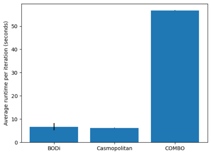
Fig. 8 shows a runtime comparison of BODi, COMBO, and CASMOPOLITAN. We show the average time to both fit the model and generate a new candidate on the MaxSAT problem with $60$ binary parameters. BODi uses the default of $128$ anchors which is used in all experiments. We observe that BODi and CASMOPOLITAN are significantly faster than COMBO and on average take less than $10$ seconds per BO iteration.

Appendix F Societal Impact

Bayesian optimization is a commonly used approach for black-box optimization across broad variety of applications, including e.g. automated machine learning (AutoML). The primary benefit of our proposed BODi method is better optimization performance for Bayesian optimization over combinatorial and mixed search spaces – in the context of AutoML this would mean finding better models or finding similarly good models while using much less computational resources. We believe that such improvements pose minimal risk beyond more general concerns about potential misuse of the underlying application.

Appendix G Dictionary construction for dictionaries with binary and categorical variables

Algorithm 4 provides pseudo-code for constructing dictionaries defined over binary input spaces $\{0,1\}^{d}$ . The key idea is to diversify the constructed dictionary by generating binary vectors determined by different bias parameters ( $\theta$ ) of the Bernoulli distribution (unlike the naive random where $\theta$ is always $1/2$ ). This algorithm is generalized to the varying-sized categorical inputs in the following way (Algorithm 5): for each of the $m$ elements of the dictionary ${\mathbb{A}}$ , we first sample a weight vector $\theta$ from the $\tau_{max}$ -simplex $\Delta^{\tau_{max}}$ , where $\tau_{max}=\max_{j}\tau_{j}$ . For each variable $v_{j}$ , we then sample $\tau_{j}$ elements from $\theta$ and use those as the weight vector of a categorical distribution from which we in turn draw the $j$ -th dimension of the dictionary element.

Algorithm 4 Dictionary design for binary input space

\{0,1\}^{d}

with diversely sparse rows

requires: dictionary size $m$

1: Dictionary

{\mathbb{A}}\leftarrow

empty

2: for

i

1,2,\ldots,m

{\mathbb{a}}_{i}\leftarrow

empty

4: Sample Bernoulli parameter

\theta\sim\text{Uniform}(0,1)

5: for

j

1,2,\ldots,d

6: Sample binary number

a\sim\text{Bernoulli}(\theta)

{\mathbb{a}}_{i}\leftarrow{\mathbb{a}}_{i}\cup a

8: end for

9: Add

{\mathbb{a}}_{i}

to dictionary:

{\mathbb{A}}\leftarrow{\mathbb{A}}\cup{\mathbb{a}}_{i}

10: end for

11: return the dictionary

{\mathbb{A}}

of size

m\times d

Algorithm 5 Dictionary design for discrete spaces with categorical variables via diverse parameters

Input: candidate sets $C(v_{1}),\dotsc,C(v_{d})$ , dictionary size $m$ Output: the dictionary ${\mathbb{A}}$ of size $m\times d$

1: Dictionary

{\mathbb{A}}\leftarrow

empty

\tau_{max}\leftarrow\max_{j}\tau_{j}

3: for

i

1,2,\ldots,m

{\mathbb{a}}_{i}\leftarrow

empty

5: Sample

\bm{\theta}\sim\Delta^{\tau_{max}}

6: for

j

1,2,\ldots,d

\bm{\theta}_{j}\leftarrow

sample (w/o repl.)

\tau_{j}

elements from

\bm{\theta}

\bm{\theta}_{j}\xleftarrow{}\bm{\theta}_{j}/\|\bm{\theta}_{j}\|_{1}

(Normalize to yield distribution)

a\leftarrow

sample from

C(v_{j})

with probabilities

\bm{\theta}_{j}

10:

{\mathbb{a}}_{i}\leftarrow{\mathbb{a}}_{i}\cup a

11: end for

12: Add

{\mathbb{a}}_{i}

to dictionary:

{\mathbb{A}}\leftarrow{\mathbb{A}}\cup{\mathbb{a}}_{i}

13: end for

Illustration of Algorithm 5

We illustrate the description in Algorithm 5 with a simple example for an input with the same number of candidate choices for each input dimension. Let’s say, we want to construct a dictionary vector for an input space with 10 variables (i.e. 10-dimensional input) where each dimension can take 4 values (i.e., $\tau_{1}=\tau_{2}….=\tau_{d}=4$ ). For each input dimension (for loop in line 6), we sample a value from a categorical distribution which is parameterized by weights $\theta_{j}$ . In the naive random case, $\theta_{j}$ is [¼, ¼, ¼, ¼ ]. In contrast, algorithm 5 diversifies this vector $\theta_{j}$ by sampling from a simplex in line 5. The variable $\tau_{max}$ (Line 2) and resampling of $\theta$ in Line 7 allows us to generalize the algorithm for the case where each input dimension can take a different number of values.

	$\displaystyle 2\\|{\bm{\phi}}_{\mathbb{A}}(\mathbf{z})-{\bm{\phi}}_{\mathbb{A}}(\mathbf{z}^{\prime})\\|$	$\displaystyle=\\|(d\mathbb{1}_{n}-\bar{{\mathbb{A}}}\bar{\mathbf{z}})-(d\mathbb{1}_{n}-\bar{{\mathbb{A}}}\bar{\mathbf{x}}^{\prime})\\|$
		$\displaystyle=\\|\bar{{\mathbb{A}}}\bar{\mathbf{z}}-\bar{{\mathbb{A}}}\bar{\mathbf{z}}^{\prime}\\|$
		$\displaystyle=\\|\bar{{\mathbb{A}}}\bar{\mathbf{r}}\\|,$