Lensing of Vacuum Entanglement near Schwarzschild Black Holes
Abstract
An important feature of Schwarzschild spacetime is the presence of orbiting null geodesics and caustics. Their presence implies strong gravitational lensing effects for matter and radiation, i.e., for excitations of quantum fields. Here, we raise the question whether the lensing manifests itself also in the vacuum of quantum fields, namely by lensing the distribution of vacuum entanglement. To explore this possibility, we use the method of entanglement harvesting, where initially unentangled localized quantum systems are temporarily coupled to the field at different locations. We find that for the Boulware, Hartle-Hawking and Unruh vacua in 3+1-dimensional Schwarzschild spacetime, the harvesting of vacuum entanglement is indeed greatly amplified near caustics. In particular, we establish that preexisting vacuum entanglement can also be harvested for lightlike separations.
I Introduction
The presence of entanglement between spatially separated degrees of freedom of a quantum field is a basic phenomenon that occurs even for free fields in the vacuum state on a flat background spacetime Summers and Werner 1985; Summers and Werner 1987. The origin of this vacuum entanglement can be traced back to the fact that, in wave equations, neighboring field oscillators must be coupled to each other in order to describe the propagation of waves. The coupling between the neighboring field oscillators is through spatial derivatives in the wave operators, such as the d’Alembertian and Dirac operator. It is this coupling between neighboring field oscillators that also causes the ground state of the local field oscillators to be an entangled state.
In curved spacetimes, curvature impacts the derivatives in the wave operators which then impact the entanglement in the field. Therefore, curvature also impacts the field correlations. Conversely, it has been shown that the imprint that curvature leaves in the field correlators is actually complete in the sense that the metric can be reconstructed from the field correlators Saravani et al. 2016; Kempf 2021. As was shown in Ref. Perche and Martín-Martínez 2022, the metric can also be reconstructed from the correlations between local measurements of the field. The entanglement structure of quantum fields plays a fundamental role in investigations of phenomena from holography to Hawking radiation and the black hole information loss problem Bekenstein 1973; Bombelli et al. 1986; Srednicki 1993; Eisert et al. 2010; Witten 2018; Hawking 1974; Hawking 1975; Davies 1975; Page 1993; Page 2013; Penington 2020.
To probe the spacetime distribution of entanglement in a quantum field, a versatile method is to couple initially unentangled localized quantum systems to the field at different spacetime regions. The amount of entanglement that the localized systems acquired can be determined by standard methods Reznik et al. 2005; Pozas-Kerstjens and Martín-Martínez 2015.
When the entanglement acquired from the field by localized quantum systems is extracted from the entanglement that was preexisting in the field, this protocol has become known as entanglement harvesting. Entanglement harvesting has been investigated in a number of scenarios since first hinted at in Refs. Valentini 1991; Reznik 2003, in both flat and curved spacetime. It has been proven that entanglement harvesting can capture the geometry VerSteeg and Menicucci 2009 and topology Martín-Martínez et al. 2016 of the underlying spacetime. So far, the scenario where entanglement is harvested from the field in the presence of black holes has only been studied in very idealized scenarios such as 2+1-dimensional (Bañados-Teitelboim-Zanelli) black holes Henderson et al. 2018 and 1+1-dimensional spacetimes with horizons Gallock-Yoshimura et al. 2021. The question of entanglement harvesting near a black hole in 3+1 spacetime dimensions has remained open. However, this case is of particular interest since one can expect new phenomenology, for example, due to lensing (see Ref. Cliche and Kempf 2011) and due to the fact that orbiting null geodesics and caustics can connect the two localized harvesting systems.
The phenomenology arising from orbiting null geodesics and caustics on communication through quantum fields close to a Schwarzschild black hole was addressed in Ref. Jonsson et al. 2020. Here, we investigate in detail entanglement harvesting in a four-dimensional Schwarzschild spacetime, for the cases of the Boulware, Hartle-Hawking and Unruh vacua, using tools similar to those applied in Ref. Jonsson et al. 2020. We take the localized quantum systems to be static localized two-level quantum systems with a monopole coupling to a Klein-Gordon field, i.e., so-called Unruh-DeWitt (UDW) detectors, or detectors for short. Within this setup, we analyze the impact of the presence of caustics and of the fact that the detectors can be connected by secondary null geodesics, including the case where detectors are placed close to the event horizon.
We find, that the presence of caustics alters the characteristics of entanglement harvesting in two particular ways in comparison to flat spacetime. First, due to a lensing-like effect caused by the focusing of null geodesics, the final entanglement between detectors can become greatly amplified near the caustics in comparison to comparably placed detectors away from caustics. Second, due to changes in the singularity structure of the Wightman function which happen when the field waves cross through caustics, we observe that timelike-separated detectors can harvest preexisting entanglement from the field if they are aligned along secondary null geodesics, i.e., null geodesics which orbit half of the black hole and so they have passed through one caustic. To the best of our knowledge, such harvesting of preexisting entanglement for lightlike separations has never been observed before in any spacetime.
Sec. II.2 begins by discussing the treatment and properties of the Wightman function of a massless scalar field on Schwarzschild spacetime and, in particular, its global singularity structure. Sec. III introduces the detector model, its perturbative treatment and negativity as entanglement measure for the detectors’ final state. Sec. III.2 discusses when the entanglement between detectors can be attributed to the harvesting of preexisting entanglement from the field. Sec. IV presents our actual results for specific detectors and the article closes in Sec. V with a discussion and outlook. The appendices collect supplemental figures. Furthermore, App. A gives the calculations of the perturbative contributions to the detectors’ state and App. B discusses the numerical techniques for the evaluation of the Wightman functions and integrals evolving the Wightman function.
We use the natural units in which .
II Wightman function in Schwarzschild spacetime
In this section we introduce a quantum scalar field in Schwarzschild spacetime as well as the Wightman function when the scalar field is in three quantum states of interest (namely, Boulware, Unruh and Hartle-Hawking). The reader familiar with these may wish to skip to Sec. II.2, reviewing literature results on the global singularity structure of the Wightman function as the field wave front passes through caustics of Schwarzschild spacetime which motivate our search for gravitational lensing of entanglement harvesting.
II.1 Klein-Gordon quantum field in Schwarzschild spacetime
In this section, we briefly review the treatment of a massless Klein-Gordon field in Schwarzschild spacetime, and the expressions for the Wightman function of the three field states we consider, which are needed for the perturbative treatment of the field-detector interaction.
The line element of the outer region of Schwarzschild spacetime in Schwarzschild coordinates , is given by
| (1) |
where is the mass of the black hole and is the radius of the event horizon. In this outer region, we consider a scalar quantum field obeying the Klein-Gordon (K-G) equation . Considering the Schwarzschild spacetime and availing of its spherical symmetry, a general real-valued solution for that equation can be written as
| (2) |
where denotes a spacetime point, are creation and annihilation operators and
| (3) |
with being the spherical harmonic of degree and order and are radial factors.
Substituting the field modes (3) into the K-G equation leads to the conclusion that obeys
| (4) |
where is the tortoise coordinate and is an effective potential.
The two linearly independent solutions and are defined by the asymptotic boundary conditions
| (5) | ||||
| (6) |
Here, are the reflection amplitudes and is the incidence amplitude. For compatibility with Ref. Candelas 1980 and ease of notation, let us also define
| (7) |
Note that it suffices to calculate the modes for just and use the following symmetries for :
| (8) |
Calculating the response of the detectors to the interaction with the quantized field requires, as we shall see in the next section, the Wightman function. The Wightman function, when the quantum field is in a state , is defined as
| (9) |
It is thus a two-point function satisfying the homogeneous K-G equation. Henceforth we shall only consider quantum states in regions of spacetime where they satisfy the Hadamard property (namely, Eq. (14), is satisfied for the Wightmant function in such states). The Wightman function in Schwarzschild spacetime is given by Candelas 1980
| (10) |
where is the angular separation between the two spacetime points and and . The integral kernel depends on the quantum state of the field. For the Boulware Boulware 1975 (), Unruh Unruh 1976 () and Hartle-Hawking Hartle and Hawking 1976 states () it takes the forms
| (11) | ||||
| (12) | ||||
| (13) |
where is the surface gravity, and denotes the (rescaled) radial factor of the ingoing and upgoing solutions to the wave equation, as defined in Eq. (7). App. B discusses the numerical techniques used for the evaluation of the Wightman function.
The expressions above convey that in the Boulware state both ingoing and upgoing modes are in their ground state, whereas in the Unruh state the upgoing modes are thermalized, and in the Hawking state both ingoing and upgoing modes are thermalized.
II.2 Singularity structure of the Wightman function
The Hadamard form for the Wightman function is an analytic expression which is defined in a local neighborhood11 1 More precisely, the Hadamard form is only defined in a normal neighborhood of : a neighbourhood of such that every is connected to by a unique geodesic which lies in . of the source point and explicitly shows its singularity structure. Explicitly, it is (e.g., Refs. Hollands and Wald 2015; DeWitt and Brehme 1960; Hadamard 1923)
| (14) |
where , and are regular and real-valued biscalars. The so-called Synge’s world function is equal to one-half of the square of the geodesic distance joining and , which implies that is negative/zero/positive whenever that geodesic is, respectively, timelike/null/spacelike. The biscalars and are uniquely determined by the geometry of the spacetime whereas in principle depends on the quantum state . The term in Eq. (14) with is called the direct part and the term with the tail part.
In order to see separately the divergences of the real and imaginary parts of the Wightman function, the following distributional limits are useful:
| (15) | ||||
| (16) |
where PV denotes the principal value distribution. This readily yields the anticommutator
| (17) |
and the commutator
| (18) |
The anticommutator and commutator (which, when multiplied by ‘’ yields the classical retarded Green function) are, respectively dependent and independent of the quantum state of the field.
Eq. (14) shows explicitly the singularity of the Wightman function along , i.e., when and a in a local neighborhood of are connected by a null geodesic. It is well known Garabedian 1998; Ikawa 2000 that the Wightman function continues to diverge when and are connected by a null geodesic globally, i.e., even when is not in a local neighborhood of . The global singularity structure of the Wightman function in the case of Schwarzschild spacetime was unveiled in Ref. Buss and Casals 2018: the divergence of follows a fourfold pattern, with the singularity type changing every time the null wave front passes through a caustic point (i.e., a spacetime point where neighboring null geodesics are focused; in Schwarzschild spacetime, because of the spherical symmetry, caustics lie along the line of the point of emission of the null geodesics as well as along the antipodal line ). Specifically, the pattern for the leading divergence in the real part of the Wightman function is22 2 An exception to the validity of Eqs. (19) and (20) is at caustic points; also, by “” in these equations we mean a well-defined extension of the world function outside normal neighborhoods – see Casals and Nolan 2016 about both of these points.
| (19) |
and that in the imaginary part of the Wightman function is
| (20) |
where we have omitted the coefficients of the singularity factors.33 3 Ref. Buss and Casals 2018 showed what the global singularity structure of the Feynman Green function is, from which that of the Wightman function readily follows. As an example, the leading singularities of the real and imaginary parts of the Wightman function along the wave front before crossing any caustics are, respectively, and (corresponding to the direct part in Eq. (14)), whereas after the wave front has crossed one caustic point these turn into, respectively, and . This change in the singularity structure will have relevant consequences in entanglement harvesting as we show below.
The above is the leading singularity structure but there is a corresponding subleading singularity structure. Ref. Casals and Nolan 2016 showed that, for the imaginary part of the Wightman function, its subleading fourfold structure is:
| (21) |
Ref. Casals and Nolan 2016 further conjectured that the subleading structure for the real part of the Wightman function is:
| (22) |
The first terms in Eqs. (21) and (22) of course correspond to, respectively, the imaginary and real parts of the tail term in Eq. (14).
III Entanglement harvesting
III.1 Detector model and perturbative treatment
Alice and Bob will carry detectors that can locally measure the field around them. To model their detectors we will use the conventional Unruh-DeWitt particle detector model DeWitt 1979; Unruh 1976, which consists of a nonrelativistic quantum system coupled locally to a scalar quantum field. The Unruh-DeWitt model is covariant and causal44 4 For pointlike detectors this is strictly true. For smeared detectors this is true in an approximated sense. For details see Refs. Martín-Martínez et al. 2021; de Ramón et al. 2021 Martín-Martínez 2015; de Ramón et al. 2021; Martín-Martínez et al. 2020; Martín-Martínez et al. 2021 and captures the main features of the light-matter interaction (e.g., atoms coupled to the electromagnetic field) when exchange of angular momentum between the field and the internal degrees of freedom of the detector is not relevant Lopp and Martín-Martínez 2021. The covariant treatment and use of time-dependent perturbation theory to calculate the joint time evolution of the detectors and the field in arbitrary curved spacetimes can be found in Refs. Martín-Martínez et al. 2020; Martín-Martínez et al. 2021. In particular, in the context of entanglement harvesting this model has been extensively used throughout the literature and the particular perturbative approach employed here will use the same notation and conventions used in, among many others, Ref. Pozas-Kerstjens and Martin-Martinez 2015. Hence, here we only give a brief summary stating the most relevant expressions for the present work.
We model the particle detectors as two-level systems with energy eigenstates (ground state) and (excited state) which are separated by an energy gap . The detectors couple to the field amplitude along their worldline through the interaction Hamiltonian55 5 In the fully covariant formulation of the interaction a Hamiltonian density is prescribed Martín-Martínez et al. 2020. For pointlike detectors, integrating this density over hypersurfaces of constant yields Eq. (23).
| (23) |
where is a coupling constant which is dimensionless in (3+1)-dimensional spacetime, is a real-valued switching function, is the detector’s proper time and is the monopole operator. Note that the Hamiltonian of (23) generates time translation with respect to coordinate time , but not the detector’s proper time . (For a detailed discussion of this point, see Refs. Martin-Martinez and Rodriguez-Lopez 2018; Martín-Martínez et al. 2020.)
In the scope of this work, we consider static detectors in Schwarzschild spacetime, i.e., detectors with constant spatial coordinates . For such detectors
| (24) |
and we choose the relation between coordinate time and detector proper time as . As switching functions for the detector we use Gaussians which as a function of coordinate time read
| (25) |
where denotes the switching width and is the center of the switching function.
We assume the initial state of the system (at ) to be a product state between the ground states of the two detectors and a field state :
| (26) |
Assuming that the field state has vanishing one-point function, the expansion of the detectors’ state after time evolution in coordinate time is
| (27) |
Using the basis order the final state is represented by the density matrix
| (28) |
whose entries are
| (29) | ||||
| (30) |
where takes complex values while takes non-negative values. For our case of static detectors and Gaussian switching functions, as shown in Eqs. (39) and (40), using the mode expansion of the Wightman function, these expressions can be solved analytically up to one integration over the frequency of the field modes which needs to be performed numerically.
To assess and quantify the entanglement of the two detectors in the final state we use its negativity. Its perturbative expansion is with
| (31) |
We see that whether the two detectors end up in an entangled state, is determined by a competition between the size of the correlating term and the local noise terms and . In particular, if the noise terms are equal, , as will be the case in Sec. IV, then the negativity and, thus, the entanglement between the detectors vanishes if , i.e., when the noise overcomes the correlations. Notice that, because and are local noise terms for which the Wightman function is evaluated along a single detector’s worldline, they contain no information about field correlations between the two regions where the two detectors are interacting with the field.
III.2 When is the entanglement extracted versus generated?
Entanglement harvesting is an interesting process because it can demonstrate the presence of entanglement in a quantum field between different spacetime regions. For example, it is clear that when two initially uncorrelated detectors become entangled through their interaction with the field while remaining spacelike separated, then the entanglement they acquire comes from “extracting” preexisiting entanglement in the field (see, e.g., Refs. Reznik 2003; Pozas-Kerstjens and Martin-Martinez 2015 in flat spacetime). However, when the detectors are not spacelike separated, contributions to the correlating term in the leading-order perturbative correction to arise which are independent of the quantum state of the field, as recently studied in Ref. Tjoa and Martín-Martínez 2021. In fact, these contributions can be calculated solely from classical data, consisting of switching functions, detector worldlines and the field classical Green function. Hence, they tell nothing about the quantum properties of the field.
To see this, we follow Ref. Tjoa and Martín-Martínez 2021. First, note that the imaginary part of the Wightman function, given by the commutator of the field operators, is independent of the state of the field. Only the real part, which is given by the anticommutator of the field operators, depends on the quantum state. We can use this to split into two contributions as , where is obtained by replacing by its real part (which is symmetric) on the right-hand side of Eq. (29), and by replacing with its imaginary part (which is antisymmetric). Note that, in general, and are complex-valued.
Below we will encounter generic scenarios where the detectors become entangled while is dominated by , and is (almost or exactly) vanishing. In such a situation most66 6 A quantitative study of the relative contributions of and to the entanglement acquired by the detectors for the case of flat spacetime can be found in Ref. Tjoa and Martín-Martínez 2021. of the entanglement between the detectors is not to be attributed to any preexisting entanglement in the field, as we shall next argue. In such a scenario the entanglement between the detectors, as measured by , would remain unchanged if we replaced the initial field state by a state which resulted in the same values for and (the value of , would also remain unchanged since it is state independent). In particular, we could replace the original state of the field by a state that has the same Wightman function within the regions where the detectors are coupled to the field, while containing no entanglement between those two regions.
Hence, in this new state, the entanglement between the detectors appears to be generated due to their sequential interaction with the field instead of being extracted from preexisting correlations in the field. This line of reasoning was used in Ref. Tjoa and Martín-Martínez 2021 in order to argue that in these cases where is (almost or exactly) vanishing, the entanglement acquired by the detectors should not be referred to as “entanglement harvesting” from the field.
In its turn, in a scenario with spacelike-separated detectors where all entanglement between the detectors is harvested from preexisting entanglement in the field, we have that because the commutator vanishes between the detectors. That is, in this clear-cut scenario, the contributions from the field’s state-dependent anticommutator are the ones that transfer the entanglement from the field to the detectors.
In addition, another observation made in Ref. Tjoa and Martín-Martínez 2021 indicates that for timelike-separated detectors the processes captured in are also due to the harvesting of preexisting entanglement in the field as opposed to generation of entanglement through the interaction. This is based on the fact that a process that creates entanglement between the detectors by having them sequentially interact with the field also allows for communication from the first to the second detector: the field carries information between the two detectors and that can get them entangled independently of any preexisting entanglement in the field. However, it is well known that at leading order in perturbation theory, with which we are concerned here, such causal influence of one detector on the other is determined by the commutator of the field and independent of the anticommutator of the field (see, e.g., Eq. (24) of Ref. Martín-Martínez 2015). Thus, as argued in Ref. Tjoa and Martín-Martínez 2021, it appears plausible that, generally, the detectors are harvesting preexisting entanglement from the field if is dominated by contributions arising from the anticommutator.
IV Harvesting of gravitationally lensed vacuum entanglement
This section contains the main results which demonstrate the impact of gravitational lensing, which at caustics refocuses null geodesics emanating from a common source, on entanglement harvesting. To this end, we consider static detectors placed close to the black hole horizon and compare their behavior with the well-studied case of static detectors in flat spacetime.
As one would expect, an important parameter that decides if and to what extent two detectors become entangled is their distance. The distance between (the static worldlines of) the two detectors can be defined in terms of various meaningful measures (see also Ref. Jonsson et al. 2020). In the present context (of static observers in Schwarzschild or Minkowski spacetime), the light propagation coordinate time is an intuitive choice of measure which we use henceforth when referring to the distance between detectors. This is the minimal amount of (Schwarzschild or Minkowski) coordinate time that it takes light to propagate from the spatial position of one detector to that of the other detector along a null geodesic.
Once the spatial positions of the two detectors are chosen and, thus, their distance is fixed, the interaction of the detectors with the field can still be made to happen at spacelike, lightlike or timelike separation by introducing a switching delay; this means that the switching function of the second detector is shifted with respect to the first one by a certain amount of coordinate time. For example, in the following we will assume that both detectors couple through the same switching function (25) and introduce the switching delay as the (coordinate time) difference between the centers of the switching functions. The switching delay can then be used to maximize the entanglement in the final state of the two detectors.
In Minkowski spacetime, as far as the impact of the switching delay is concerned, the entanglement in the final state between two detectors at a fixed distance is maximized when the switching functions are exactly null aligned Tjoa and Martín-Martínez 2021, i.e., when the switching delay equals the light propagation time.77 7 This statement is not entirely precise, as in Minkowski spacetime the maximum is located very close to–but not exactly at–null alignment of the switching functions, see Ref. Tjoa and Martín-Martínez 2021. As far as the impact of the distance between the detectors is concerned, its impact on the final entanglement is straightforward: if the distance between the detectors is increased (while allowing the switching delay to be optimal and leaving other coupling parameters unchanged), the entanglement between the detectors in their final state decreases and goes to zero beyond a certain distance. This holds even if the switching delay is readjusted to uphold null alignment. Furthermore, in 3+1-dimensional Minkowski spacetime, the entanglement between exactly null aligned detectors is dominated by correlations generated by communication rather than by harvesting, because the term is dominated by rather than , as shown in Ref. Tjoa and Martín-Martínez 2021.
This raises two questions regarding entanglement harvesting in Schwarzschild spacetime. First, does the presence of caustics enhance the ability of detectors to become entangled? What is more, can caustics make the harvested entanglement no longer decrease monotonically with distance?
Second, does the singularity structure of the Wightman function allow for the entanglement to be dominated by harvesting rather than signaling if the detectors’ switching instead of being aligned along a direct null geodesic is aligned along a secondary null geodesic, i.e., a null geodesic that has passed through a caustic? As discussed in Sec. II.2, here the singularity structures of the real and imaginary parts of the Wightman function are shifted, so that could dominate over because the real part now carries the -singularity. This would then constitute entanglement harvesting between timelike-separated detectors, since the secondary null geodesics lie inside the causal cone which is bounded by the direct null geodesics between detectors.
The following results answer both questions in the affirmative.
Fig. 1 shows the gravitational lensing effect on the harvesting of entanglement by two static detectors in Schwarzschild spacetime when the field is in the Boulware state. The scenario is as follows. Two identical detectors, with detector gap and ,88 8 Note that because is dimensionless and all terms are of order the numeric value of only affects the result by an overall factor. We choose for improved readability. are placed on static worldlines at the same radial coordinate . The angular separation between the two detectors varies along the horizontal axes of each panel. Both detectors are coupled to the field through the Gaussian switching function (25), but the difference between the two centers of the switching functions is shifted by an amount of coordinate time which varies between the panels as indicated.
An inset in each panel visualizes how far null geodesics, emanating from detector a at time , propagate within the coordinate time interval : the black filled circle represents the interior of the black hole horizon at , a black ring around it represents all points with radial coordinate and the red dot represents the spatial location of detector a. The violet curve then indicates the spatial position of the null wave front after propagation time . In particular, the different insets show the formation of caustics located at angular separation from the point of origin (which is plotted in red) where the null wave front intersects itself. The caustic reaches at .
The four different curves in each panel show the resulting contributions to the final density matrix of the two detectors (28), when the field is in the Boulware state. (Accordingly they are denoted with a superscript .) The horizontal, red and dashed line shows the single detector noise term . Because it only depends on the radial coordinate and the switching function’s width , it is equal for both detectors and constant for all positions of detectors considered here.The blue solid curve shows the absolute value resulting from the chosen value of the switching delay in each panel, as a function of the angular separation between the detectors. The two remaining dashed curves show the absolute values in green and in orange which, as discussed in Sec. III.2, are obtained by replacing the Wightman function by its imaginary and real parts, respectively. In particular, as discussed in Sec. III.2, if is dominated by (obtained from the imaginary part), then the detectors’ entanglement is predominantly generated in the sequential interaction of the detectors with the field. On the other hand, if is dominated by then final entanglement between the detectors is predominantly harvested from preexisting entanglement in the vacuum of the field.
Altogether the panels in Fig. 1 illustrate the lensing effect which appears in proximity to the caustics. The first two panels show the settings with the shortest switching delay between the switching functions. In these two plots, we see that the correlations between the detectors, as captured by , are largest when the centers of the intervals during which the detectors couple to the field are connected by (direct) null geodesics. In the first panel there is a certain interval of angular separations in which the blue line for exceeds the noise term and the detectors end up entangled. However, in the second panel the detectors’ final state remains separable, even for null separated detectors, because is increased. Note that here the contribution from dominates the peaks of ; hence entanglement between the detectors cannot be attributed to harvesting of preexisting entanglement from the field but to entanglement generation due to sequential interaction.
In flat spacetime no entanglement would be observed in the final detectors’ state for larger switching delay between the detectors. Intuitively this is related to the growth of the light cone’s surface area which dilutes the entanglement. In Schwarzschild spacetime, however, where the light cone refocuses at caustics the opposite can happen. As seen in the third through sixth panels (in order of increasing ), the detectors can become entangled at larger switching delays again, at angular separations close to in the proximity of caustics. This answers in the affirmative the first of the two guiding questions raised above.
The second of the two questions raised above pertains to the Wightman function’s singularity structure described in Sec. II.2. Its effect is easy to recognize when comparing the last (bottom right) panel to the first (top left) panel of Fig. 1. In both panels the correlations between the two detectors, as captured by , are maximal for null aligned detectors. However, in the first panel the detectors are connected by primary null geodesics, whereas in the last panel they are connected by secondary null geodesics. At secondary null geodesics, as discussed in Sec. II.2, the singularity structure of the Wightman function is shifted from primary null geodesics so that now the real (anticommutator) part carries the -singularity, which used to be carried instead by the imaginary (commutator) part in the case of primary null geodesics. Accordingly, the two contributions have a qualitatively similar overall shape in the first and the last panels, except that the and have swapped places. For detectors aligned along a secondary null geodesic, the real part contribution dominates over the imaginary part contribution . So if these correlations overcame the noise, , the detectors would become entangled by harvested entanglement. However, the correlations in the last panel are too weak for the detectors to end up entangled. To find detectors that get entangled by genuinely harvested correlations around secondary null geodesics, we need to position the detectors closer to caustics so as to make use of the overall enhancement of the Wightman function there. Such a setting is seen in the fifth panel (for ) of Fig. 1. In this and the following panels of Fig. 1, the switching delay is larger than the shortest light propagation (Schwarzschild coordinate) time between detectors with angular separation , and the detectors (at ) which are null aligned here are aligned along a secondary null geodesic and timelike separated. With this we have answered in the affirmative the second of the above questions, as we observe the genuine harvesting of preexisting entanglement from the field by timelike-separated detectors, aligned along secondary null geodesics. In the following, we will see further examples allowing for entanglement harvesting between timelike-separated detectors with angular separation .
Complementary to Fig. 1, the same scenario and effects are seen in Fig. 2 from a slightly different perspective. Here, the contributions to the detectors’ final density matrix are plotted over the coordinate time switching delay , while the four different panels correspond to four different angular separations. (Fig. 6 provides a logarithmic plot of the same data.) Note that these plots over are directly comparable to the plots also found in Ref. Tjoa and Martín-Martínez 2021 in 3+1-dimensional Minkowski spacetime.
In the first panel of Fig. 2, for angular separation , there are three peaks appearing in which correspond to an alignment of the switching functions along primary, secondary and tertiary null geodesics, respectively. The qualitative structure of the first peak and its contributions from and correspond to the structure found in flat spacetime in Ref. Tjoa and Martín-Martínez 2021. However, in the secondary peak the qualitative roles of and are interchanged due to the shifted singularity structure of the Wightman function, as is easy to see in the logarithmic plot in Fig. 6. For the tertiary peak, together with the singularity structure of the Wightman function, the qualitative structure of the peak also shifts back to its primary form.
Even if there are three peaks appearing at angular separation , only the first one corresponding to alignment along the direct, primary null geodesic exhibits entanglement in the detectors’ final state. In an intermediate regime of angular separations, for , not even the primary peak overcomes the noise and the detectors’ final state remains separable for all switching delays . An example of this is seen in the third (bottom left) panel of Fig. 2 for angular separation . However, as the angular separation approaches both the primary and secondary peaks increase their size again and they overcome the noise, thus, leaving the detectors in an entangled state. Gradually, as , the primary and secondary peaks superpose and finally create one joint peak aligned at the caustic for . Here we see that for switching delays that are somewhat larger than the direct null alignment, the extracted entanglement can be dominated by and thus can be attributed to entanglement harvesting from the field.
| State | Local noise term |
|---|---|
| Boulware state | |
| Unruh state | |
| Hartle-Hawking state |
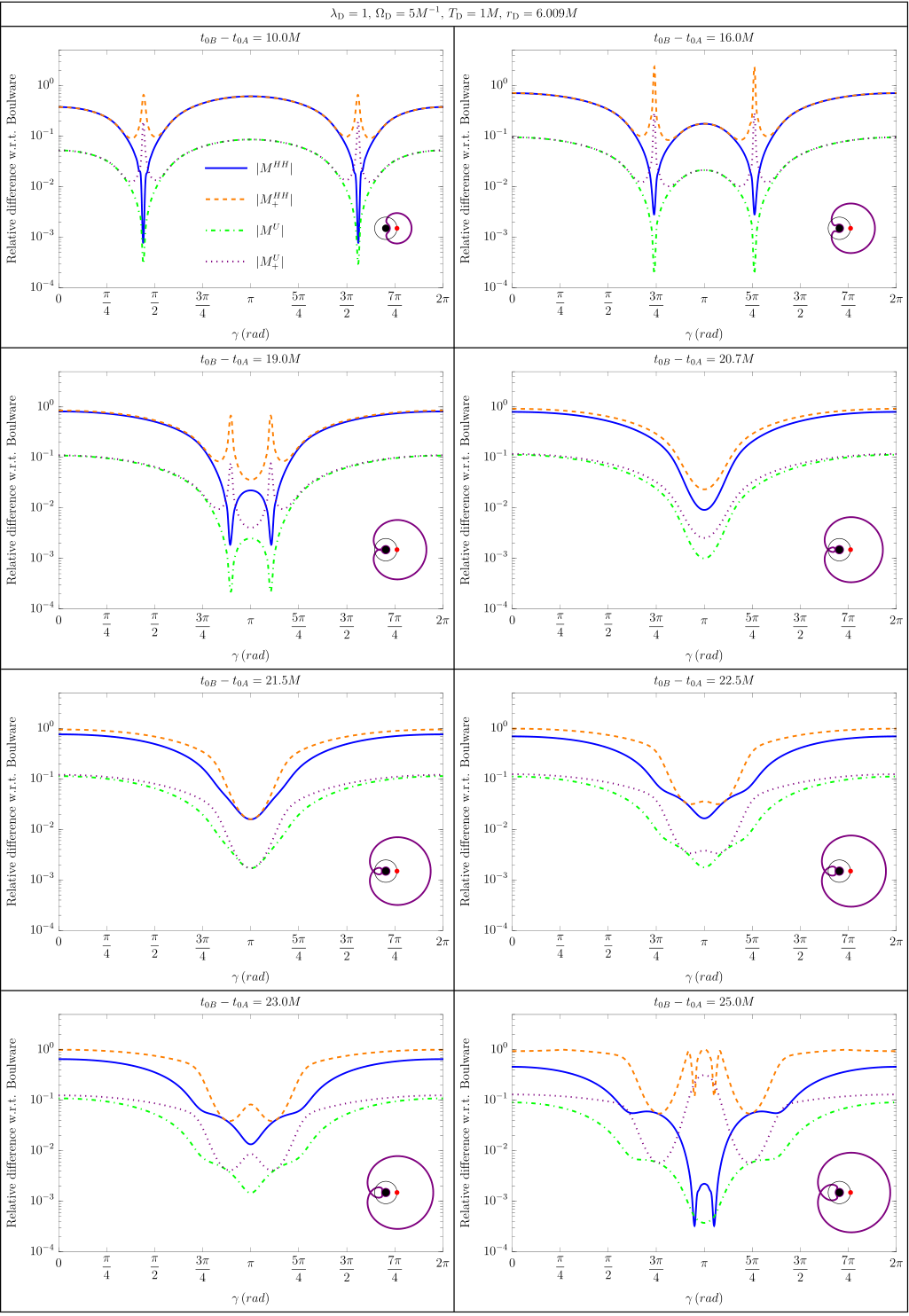
The results shown in Fig. 1 are for the field in the Boulware state. As seen in the analogous Fig. 7 for the Unruh state and Fig. 8 for the Hartle-Hawking state, the same phenomena appear in these states as well. In fact, the quantitative differences between the states (which may be difficult to see with the naked eye) are mostly due to the difference in the noise term, which is given in Tab. 1. The correlation terms, in particular in the scenarios of detectors that harvest entanglement in the proximity of caustics, agree to many digits for all three states, as can be seen in Fig. 3, which shows their relative differences.
We conclude this section with a study of entanglement harvesting from the Boulware state between detectors at antipodal locations with the black hole exactly in the middle between them, i.e., at identical radial coordinates and with an angular separation , for a range of detector locations reaching down very close to the horizon at radial positions .
At the different radial coordinates the detectors experience different gravitational redshifts. To account for this, we adjust the width of the switching functions (25) to , such that, at all radial coordinates , corresponds to the same amount of proper time given by some value . Analogous to the plots above, Fig. 4 shows the resulting contributions to the detectors’ final state for . It shows that at all radial coordinates considered, even close to the horizon, the two detectors can become entangled and the entanglement can be dominated by entanglement harvesting, when the switching delay is chosen appropriately.
To understand the structure of the plots and its dependence on it is useful to consider the light propagation coordinate time between the two detectors. This is the coordinate time that it takes for a null geodesic starting at spatial coordinates to reach the antipodal point . Fig. 5 shows this time for the range of radial coordinates we consider. It shows that is minimal at . For this critical case, it takes the value . Setting the switching delay equal to the light propagation time, i.e., setting , yields exact null alignment of the detectors’ switching functions.
Around exact null alignment between the detectors we expect a peak in the final detector entanglement, and this is, indeed, what we observe in Fig. 4. At first, in the panels showing the lower values of , one peak forms around since the detectors located at this radial coordinate are the first to be exactly null aligned. As is increased in the following panels, a double-peak structure forms since for there are always two radial coordinate positions at which the detectors are exactly null aligned. Regarding the relative size of the contributions and , we observe again that both contributions are of comparable size when the detectors are exactly null aligned, as we already observed in the panel of Fig. 2, for . This is in contrast to scenarios where the detectors are null aligned along primary null geodesics and sufficiently far away from any caustics. There, just as in flat Minkowski spacetime, the correlations are dominated by the contribution when the detectors are exactly null aligned. However, at the caustics, where a whole envelope of null geodesics connects the detectors at once, the singularity structure of the two-point function is altered (see Ref. Casals and Nolan 2016). This results in the contribution dominating before exact null alignment and the contribution dominating after exact null alignment of the switching functions.
V Discussion and outlook
Using UDW detectors, we investigated entanglement harvesting from a Klein-Gordon field in the Boulware, Hartle-Hawking and Unruh vacuum states in the background of Schwarzschild spacetime in 3+1 dimensions. We showed that the realistic 3+1-dimensional case possesses a particularly rich phenomenology due to the presence of secondary (and higher) null geodesics and caustics.
In particular, we investigated the ability of two detectors that are static at the same radial coordinate, but with different angular coordinates, to harvest entanglement from the Boulware, Hartle-Hawking and Unruh vacua as they get closer to the horizon.
We paid special attention to entanglement harvesting in the regions of spacetime where secondary null geodesics and caustics can connect the two harvesting detectors. We found that genuine entanglement harvesting can indeed be amplified through “entanglement gravitational lensing” effects when the detectors are close to regions where caustics appear. By the term “genuine entanglement harvesting” we mean the extraction of preexisting entanglement from the field, as opposed to the extraction of entanglement that is created through communication between the detectors. Interestingly, this genuine harvesting can also appear for timelike-separated detectors, for example, when the detectors are connected by secondary null geodesics. Mathematically, this results from a change in the singularity structure of the Wightman function as the field waves cross through caustics.
The formalism that we developed here can also be used to analyze further interesting black hole entanglement harvesting configurations, such as the case where the detectors are in motion and possibly also when crossing the event horizon.
Furthermore, since the effects of entanglement harvesting amplification that we found here are due to lensing which arises from the existence of secondary null geodesics connecting the two detectors, an intriguing follow-up question arises: to what extent could entanglement harvesting be engineered to be amplified even in flat spacetime, namely in the presence of suitable mirror and lensing arrangements? These scenarios will be explored in future work.
Acknowledgments
J.G.A.C. acknowledges financial support by CNPq (Brazil), Grant number 1424412/2019-8. R.H.J. gratefully acknowledges support by the Wenner-Gren Foundations and, in part, by the Wallenberg Initiative on Networks and Quantum Information (WINQ). Nordita is supported in part by NordForsk. M.C. acknowledges partial financial support by the Scientific Council of the Paris Observatory during a visit. E.M.M. acknowledges support through the Discovery Grant Program of the Natural Sciences and Engineering Research Council of Canada (NSERC). EMM also acknowledges support of his Ontario Early Researcher award. A.K. acknowledges support through a Discovery Grant from the National Science and Engineering Research Council of Canada (NSERC) and a Discovery Project Grant from the Australian Research Council (ARC).
Appendix A Density matrix contributions
In this appendix, we give a detailed derivation of the expressions used for the calculation of the perturbative contributions to the final density state of the two detectors in Eq. (28). To evaluate the leading-order contributions to the detectors’ final density matrix, we need certain Fourier-type integrals of the switching function (25), . First, we have
| (32) | ||||
| (33) |
where . Furthermore, we need the integral
| (34) |
To this end, consider
| (35) |
For the -integral, use Eqs. (A3) and (A7) from Ref. Pozas-Kerstjens and Martin-Martinez 2015, which is
| (36) |
where , with , and , then
| (37) |
Inserting this above yields
| (38) |
Appendix B Numerical techniques for the Wightman function
(b) Relative difference between the integral in Eq. (45) for the Boulware state when integrated up to and up to , with . The reason to limit this plot to is that those integrals where evaluated to ten significant digits; hence, a relative difference of means that the integral converged completely to all significant digits. Comparing with Fig. 9a, we see that exponentially fast convergence happens after becomes slightly larger than the where the asymptotic regime begins.
(c) Summand in Eq. (45) as a function of for the Boulware state. One can notice from this figure that the summand decays superexponentially with increasing . In fact, for , it has already converged to all 10 significant digits that we got when evaluating the integrals.
(d) Relative difference between the -sum in Eq. (45) for the Boulware state when summed up to and . The reason to limit this plot to is that the integrals in the sums were to 10 digits of precision. Hence, a relative difference that is smaller than should represent numerical noise and not actual significant digits.
In order to evaluate the Wightman function in the situations presented in this work, integrals over with respect to are needed. However, there is no known closed-form expression for . Hence, one has to use numerical techniques. Specifically, we use numerical methods to evaluate , and the set of coefficients in the region in steps of , in steps of and for all (integer) values . Different techniques are involved in the evaluation.
For we used the NDSolve-based numerical method implemented in the Regge-Wheeler Mathematica Wolfram Research, Inc. package of the Black Hole Perturbation Toolkit BHP.
For we define two auxiliary quantities and , then use the so-called Jaffé series Leaver 1986 to write the solution to (4) for as
| (41) |
where
| (42) | ||||
with and . This solution is implemented in Mathematica. However some care has to be taken: in practice we have to impose a cutoff on the number of terms to include in the series. To set an adequate value for we used the following quantity:
| (43) |
Since we want to have at least digits of precision in the modes, we want to find an such that
| (44) | ||||
for all values of , and in the region where the solutions are evaluated. For that, we use the fact that the convergence of the series becomes slower with increasing to conclude that the largest happens at the highest we intended to evaluate, which is around . Then, fixing we test a couple of and values in the region of interest and conclude that is enough to satisfy Eq. (44) in all regions of interest.
For the coefficients we use data from Ref. Buss and Casals 2018, which is evaluated using a Mathematica implementation of the Mano-Suzuki-Takasugi method. An extensive review of that method can be found in Ref. Sasaki and Tagoshi 2003.
B.1 -terms
By setting in Eq. (39) and manipulating the integration range from to , we obtain the following expression for the -terms:
| (45) |
To verify the convergence of such an integral, one should check the large- behavior of the , which varies among the quantum states (11)-(13):
| (46) | ||||
The leading asymptotic behavior of as is Levi and Ori 201699 9 Such asymptotics are nonuniform and valid only when , as illustrated in Fig. 9a. Hence, to leading order for large , . By substituting such a result into the integrand in Eq. (45), one concludes that the slowest-decaying term of the integrand falls off as . Therefore, the integral in Eq. (45) is fast-converging. Given that, we are able to numerically evaluate it accurately enough with a frequency cutoff . The asymptotic regime of the integrand and the convergence of the integral are illustrated in Figs. 9a and 9b.
In order to verify the convergence of the -sum, we begin by evaluating the integrals in Eq. (45), multiplying by and plotting the result against . The outcome is shown in Fig. 9c, where we can see that such a quantity decays superexponentially. Given this numerical evidence, the -sum in that equation is expected to converge with a good accuracy even with a cutoff lower than the we use. In fact, as presented in Fig. 9d, is enough to converge to all ten significant digits used when evaluating the Boulware integrals.

(b) Relative difference in the Boulware state integral in Eq. (40) after rewriting the integral so that it ranges from to for several different . To evaluate the relative difference, we integrate up to and then to , with .
(c) Boulware state integral in Eq. (40), after rewriting the integral so that it ranges from to for several different , here integrated up to .
(d) Relative difference in the Boulware state integral from (40), after rewriting the integral so that it ranges from to for several different . To evaluate the relative difference, we sum up to and then to , ranging form up to . For all significant digits exactly cancel out when evaluating the relative difference.
B.2 -terms
Since we already know the large- asymptotics of , to analyze the behavior of the integrand in Eq. (40) in that regime we have to study the factors that multiply each of its terms. These factors are very similar and it suffices to analyze only one of them:
| (47) |
where . Expanding the exponential functions, we obtain
| (48) |
where
| (49) |
Now we use an asymptotic expression for the ,
| (50) |
to conclude that as ,
| (51) |
where
| (52) |
Putting everything together we conclude that
| (53) |
which leads to the conclusion that, whenever , the whole term decays superexponentially as . On the other hand, if , which is the case we study in this work, (53) simplifies to
| (54) |
Then both, the real and imaginary parts of this quantity decay linearly with , since the absolute value of the denominator grows linearly with the frequency. Given that, by considering the extra in the integrand in Eq. (40), we conclude that it decays as . Hence, the integrals defining the -terms are convergent.
We remark that such leading asymptotic behavior in Eq. (54) is, in general, not achieved by , but one can still perform the numerical integration to a good accuracy because, before this leading asymptotic regime, there is an intermediary regime where the integrand is exponentially decaying, as can be seen in Fig. 10a. We can further confirm that convergence by looking at the integral in Eq. (40) as a function of : as can be seen in Fig. 10b, up to we have convergence up to four significant digits, while for larger values of , the convergence becomes worse, resulting in no significant digits at all. Yet, since the resulting integral decays superexponentially with , as presented in Fig. 10c, one can still obtain up to four significant digits, as can be seen in Fig. 10d.
References
- Summers and Werner (1985) S. J. Summers and R. Werner, “The vacuum violates bell’s inequalities,” Phys. lett., A 110, 257–259 (1985).
- Summers and Werner (1987) S. J. Summers and R. Werner, “Bell’s inequalities and quantum field theory. i. general setting,” Journal of Mathematical Physics 28, 2440–2447 (1987).
- Saravani et al. (2016) M. Saravani, S. Aslanbeigi, and A. Kempf, “Spacetime curvature in terms of scalar field propagators,” Physical Review D 93, 045026 (2016).
- Kempf (2021) A. Kempf, “Replacing the notion of spacetime distance by the notion of correlation,” Frontiers in Physics 9, 655857 (2021).
- Perche and Martín-Martínez (2022) T. R. Perche and E. Martín-Martínez, “Geometry of spacetime from quantum measurements,” Phys. Rev. D 105, 066011 (2022).
- Bekenstein (1973) J. D. Bekenstein, “Black holes and entropy,” Phys. Rev. D 7, 2333–2346 (1973).
- Bombelli et al. (1986) L. Bombelli, R. K. Koul, J. Lee, and R. D. Sorkin, “Quantum source of entropy for black holes,” Phys. Rev. D 34, 373–383 (1986).
- Srednicki (1993) M. Srednicki, “Entropy and area,” Phys. Rev. Lett. 71, 666–669 (1993).
- Eisert et al. (2010) J. Eisert, M. Cramer, and M. B. Plenio, “Colloquium: Area laws for the entanglement entropy,” Rev. Mod. Phys. 82, 277–306 (2010).
- Witten (2018) E. Witten, “APS Medal for Exceptional Achievement in Research: Invited article on entanglement properties of quantum field theory,” Rev. Mod. Phys. 90, 045003 (2018).
- Hawking (1974) S. W. Hawking, “Black hole explosions,” Nature 248, 30–31 (1974).
- Hawking (1975) S. W. Hawking, “Particle creation by black holes,” Communications in Mathematical Physics 43, 199–220 (1975).
- Davies (1975) P. C. W. Davies, “Scalar particle production in Schwarzschild and Rindler metrics,” J. Phys. A 8, 609–616 (1975).
- Page (1993) D. N. Page, “Information in black hole radiation,” Phys. Rev. Lett. 71, 3743–3746 (1993).
- Page (2013) D. N. Page, “Time dependence of Hawking radiation entropy,” J. Cosmol. Astropart. Phys. 2013, 028–028 (2013).
- Penington (2020) G. Penington, “Entanglement wedge reconstruction and the information paradox,” J. High Energy Phys. 2020, 2 (2020).
- Reznik et al. (2005) B. Reznik, A. Retzker, and J. Silman, “Violating Bell’s inequalities in vacuum,” Phys. Rev. A 71, 042104 (2005).
- Pozas-Kerstjens and Martín-Martínez (2015) A. Pozas-Kerstjens and E. Martín-Martínez, “Harvesting correlations from the quantum vacuum,” Phys. Rev. D 92, 064042 (2015).
- Valentini (1991) A. Valentini, “Non-local correlations in quantum electrodynamics,” Phys. Lett. A 153, 321 – 325 (1991).
- Reznik (2003) B. Reznik, “Entanglement from the vacuum,” Foundations of Physics 33, 167–176 (2003).
- VerSteeg and Menicucci (2009) G. VerSteeg and N. C. Menicucci, “Entangling power of an expanding universe,” Phys. Rev. D 79, 044027 (2009).
- Martín-Martínez et al. (2016) E. Martín-Martínez, A. R. H. Smith, and D. R. Terno, “Spacetime structure and vacuum entanglement,” Phys. Rev. D 93, 044001 (2016).
- Henderson et al. (2018) L. J. Henderson, R. A. Hennigar, R. B. Mann, A. R. H. Smith, and J. Zhang, “Harvesting entanglement from the black hole vacuum,” Classical and Quantum Gravity 35, 21LT02 (2018).
- Gallock-Yoshimura et al. (2021) K. Gallock-Yoshimura, E. Tjoa, and R. B. Mann, “Harvesting entanglement with detectors freely falling into a black hole,” Phys. Rev. D 104, 025001 (2021).
- Cliche and Kempf (2011) M. Cliche and A. Kempf, “Vacuum entanglement enhancement by a weak gravitational field,” Physical Review D 83, 045019 (2011).
- Jonsson et al. (2020) R. H. Jonsson, D. Q. Aruquipa, M. Casals, A. Kempf, and E. Martín-Martínez, “Communication through quantum fields near a black hole,” Physical Review D 101, 125005 (2020).
- Candelas (1980) P. Candelas, “Vacuum polarization in Schwarzschild spacetime,” Physical Review D 21, 2185–2202 (1980).
- Boulware (1975) D. G. Boulware, “Spin-1 2 quantum field theory in Schwarzschild space,” Phys. Rev. D 12, 350 (1975).
- Unruh (1976) W. G. Unruh, “Notes on black-hole evaporation,” Phys. Rev. D 14, 870–892 (1976).
- Hartle and Hawking (1976) J. B. Hartle and S. W. Hawking, “Path-integral derivation of black-hole radiance,” Phys. Rev. D 13, 2188 (1976).
- Hollands and Wald (2015) S. Hollands and R. M. Wald, “Quantum fields in curved spacetime,” Physics Reports 574, 1–35 (2015), quantum fields in curved spacetime.
- DeWitt and Brehme (1960) B. S. DeWitt and R. W. Brehme, “Radiation damping in a gravitational field,” Ann. Phys. 9, 220–259 (1960).
- Hadamard (1923) J. Hadamard, Lectures on Cauchy’s Problem in Linear Partial Differential Equations (Dover Publications, 1923).
- Garabedian (1998) P. R. Garabedian, Partial Differential Equations (Chelsea Pub Co, New York, 1998).
- Ikawa (2000) M. Ikawa, Hyperbolic partial differential equations and wave phenomena. Iwanami series in modern mathematics. Translations of mathematical monographs (American Mathematical Soc., Providence, 2000).
- Buss and Casals (2018) C. Buss and M. Casals, “Quantum correlator outside a Schwarzschild black hole,” Phys. Lett. B 776, 168 – 173 (2018).
- Casals and Nolan (2016) M. Casals and B. Nolan, “Global Hadamard form for the green function in Schwarzschild space-time,” (2016), arXiv:1606.03075 .
- DeWitt (1979) B. S. DeWitt, “Quantum gravity: The new synthesis,” in General Relativity : An Einstein Centenary Survey, edited by S. Hawking and W. Israel (Cambridge University Press, Cambridge Eng; New York, 1979) p. 680.
- Martín-Martínez et al. (2021) E. Martín-Martínez, T. R. Perche, and B. d. S. L. Torres, “Broken covariance of particle detector models in relativistic quantum information,” Phys. Rev. D 103, 025007 (2021).
- de Ramón et al. (2021) J. de Ramón, M. Papageorgiou, and E. Martín-Martínez, “Relativistic causality in particle detector models: Faster-than-light signaling and impossible measurements,” Phys. Rev. D 103, 085002 (2021).
- Martín-Martínez (2015) E. Martín-Martínez, “Causality issues of particle detector models in QFT and quantum optics,” Physical Review D 92, 104019 (2015).
- Martín-Martínez et al. (2020) E. Martín-Martínez, T. R. Perche, and B. de S. L. Torres, “General relativistic quantum optics: Finite-size particle detector models in curved spacetimes,” Phys. Rev. D 101, 045017 (2020).
- Lopp and Martín-Martínez (2021) R. Lopp and E. Martín-Martínez, “Quantum delocalization, gauge, and quantum optics: Light-matter interaction in relativistic quantum information,” Phys. Rev. A 103, 013703 (2021).
- Pozas-Kerstjens and Martin-Martinez (2015) A. Pozas-Kerstjens and E. Martin-Martinez, “Harvesting correlations from the quantum vacuum,” Physical Review D 92, 064042 (2015).
- Martin-Martinez and Rodriguez-Lopez (2018) E. Martin-Martinez and P. Rodriguez-Lopez, “Relativistic Quantum Optics: On the relativistic invariance of the light-matter interaction models,” Physical Review D 97, 105026 (2018).
- Tjoa and Martín-Martínez (2021) E. Tjoa and E. Martín-Martínez, “When entanglement harvesting is not really harvesting,” Physical Review D 104, 125005 (2021).
- (47) Wolfram Research, Inc., “Mathematica, Version 13.2,” Champaign, IL, 2022.
- (48) “Black Hole Perturbation Toolkit,” (bhptoolkit.org).
- Leaver (1986) E. W. Leaver, “Solutions to a generalized spheroidal wave equation: Teukolsky’s equations in general relativity, and the two‐center problem in molecular quantum mechanics,” Journal of Mathematical Physics 27, 1238–1265 (1986).
- Sasaki and Tagoshi (2003) M. Sasaki and H. Tagoshi, “Analytic Black Hole Perturbation Approach to Gravitational Radiation,” Living Reviews in Relativity 6, 6 (2003).
- Levi and Ori (2016) A. Levi and A. Ori, “Mode-sum regularization of in the angular-splitting method,” Phys. Rev. D 94, 044054 (2016).