May 2020 \thesistypePhD Thesis \imprintStockholm, Sweden, 2020 \isbnISBN: 978-91-7873-503-7 \tritaTRITA-EECS-AVL-2020:20 \publisherUniversitetsservice US AB \defenseplace \degree
Planning and Control of Uncertain Cooperative Mobile Manipulator-Endowed Systems under Temporal-Logic Tasks
Abstract
Control and planning of multi-agent systems is an active and increasingly studied topic of research, with many practical applications such as rescue missions, security, surveillance, and transportation. This thesis addresses the planning and control of multi-agent systems under temporal logic tasks. The considered systems concern complex, robotic, manipulator-endowed systems, which can coordinate in order to execute complicated tasks, including object manipulation/transportation. Motivated by real life scenarios, we take into account high-order dynamics subject to model uncertainties and unknown disturbances. Our approach is based on the integration of tools from the areas of multi-agent systems, intelligent control theory, cooperative object manipulation, discrete abstraction design of multi-agent-object systems, and formal verification.
The first part of the thesis is devoted to the design of continuous control protocols for the cooperative object manipulation/transportation by multiple robotic agents, and the relation of rigid cooperative manipulation schemes to multi-agent formation. We propose first a variety of centralized and decentralized control algorithms that do not employ force/torque information at the contact points and take into account both cases of rigid and rolling grasping points, dynamic uncertainties in the object’s and agents’ model, and potential constraint satisfaction, such as obstacle avoidance and input saturation. Next, we tackle the problem of robust formation control for a class of multi-agent systems and we analyze the relation between formation rigidity theory and rigid cooperative manipulation.
In the second part of the thesis, we develop control schemes for the continuous coordination of multi-agent complex systems with uncertain dynamics. We first study the motion planning problem and propose novel adaptive control schemes for the collision-free navigation of single- and multi-agent spherical systems in obstacle-cluttered environments. Next, we focus on the leader-follower coordination problem of spherical multi-agent systems. More specifically, we design a robust adaptive decentralized control scheme for the successful navigation of a designated leader to a predefined point, while guaranteeing collision avoidance and connectivity maintenance properties. Finally, we design a closed-form robust barrier function-based control protocol for the collision avoidance of multiple D ellipsoidal agents.
The third part of the thesis is focused on the planning and control of multi-agent and multi-agent-object systems subject to complex tasks expressed as temporal logic formulas. We tackle first the case of local independent tasks for multi-agent systems, and by using previous results on multi-agent constrained navigation, we design a discrete abstraction of the agents’ motion in the workspace and synthesize decentralized control policies that satisfy the agents’ specifications. Next, in addition to the robotic agents, we take into account complex tasks to be satisfied by unactuated objects. We design a discrete abstraction that simulates the behavior of the agents and the objects in the workspace and we synthesize controllers for the agents that take into account both theirs and the objects’ specifications.
The fourth and final part of the thesis focuses on several extension schemes for single-agent setups. Firstly, we consider the problem of single-agent motion planning under timed temporal tasks in an obstacle-cluttered environment. Using previous results on collision-free timed navigation, we develop a novel control policy that guarantees satisfaction of the agent’s timed tasks as well as asymptotic optimality with respect to energy resources. Secondly, we tackle the motion planning problem for high-dimensional complex systems with uncertain dynamics in obstacle-cluttered environments. We integrate intelligent control techniques with sampling-based motion planning algorithms to guarantee the safe navigation of the system to a predefined goal, while compensating for the model inaccuracies. Finally, we develop a novel control protocol that achieves asymptotic reference tracking for an unknown control affine system, while respecting at the same time funnel constraints.
Sammanfattning
Reglering och planering av multiagent-system är ett aktivt och växande forskningsfält med en rad praktiska tillämpningar såsom räddningsuppdrag, övervakning, säkerhet och transport. Denna avhandling adresserar planering och reglering av multiagent-system med temporallogiska uppgifter. De berörda systemen är komplexa, robotiska, manipulatorbaserade system, vilka kan samarbeta för att utföra komplicerade uppgifter, bland annat manipulation och transport av objekt. Motiverade av verkliga scenarier tar vi hänsyn till högnivå dynamik med osäkerheter och okända störningar. Vårt angreppssätt baseras på integration av redskap från följande områden: multiagent-system, intelligent reglerteknik, samarbetande objekt-manipulation, diskret abstrakt design av multi-agent-objekt system och formell verifiering.
Avhandlingens första del tillägnas design av kontinuerliga protokoll för samarbetande manipulering och transportering av objekt utförd av flera robotagenter, och relationen av rigida samarbetskrävande manipulationsuppgifter. Vi föreslår först några centraliserade och decentraliserade regleralgoritmer som saknar information om kraft och moment i kontaktpunkterna, men som tar hänsyn till både fasta och rullande greppunkter, dynamiska osäkerheter i objektets och agentens modell, samt möjlighet till att uppfylla villkor såsom att undvika hinder och mättning av insignaler. Som ett nästa steg behandlar vi reglering för robust formering för en klass av multi-agent system och vi analyserar relationen mellan teori för formationsrigiditet och rigid samarbetskrävande manipulation.
I avhandlingens andra del utvecklar vi regleralgoritmer för kontinuerlig koordinering av komplexa multi-agent system med osäker dynamik. Vi betraktar först rörelseplanering och föreslår nya adaptiva regleralgoritmer för kollisionsfri navigering av enkel- och sfäriska- multiagent-system i hinderfyllda miljöer. Vi fokuserar sedan på ledar-följare koordinering av sfäriska multiagent-system. Mer specifikt så designar vi robust adaptiv decentraliserad reglering för framgångsrik navigation av en utnämnd ledare till en förutbestämt punkt, samtidigt som vi garanterar att kollisioner kan undvikas och att sammankoppling upprätthålls. Slutligen designar vi ett robust reglerprotokoll på återkopplad form baserat på barriärfunktion för kollisionsundvikande av multipla ellipsoidformade 3D-agenter.
Avhandlingens tredje del fokuserar på planering och reglering av multiagent och multiagent-objekt system med komplexa uppgifter uttryckta med formler på temporallogisk form. Vi behandlar först fallet med lokala oberoende uppgifter för multiagent-system, och genom att använda tidigare resultat från begränsad navigering av multiagent-system designar vi en diskret abstraktion av agentens rörelse i arbetsytan och syntetiserar decentraliserade reglerpolicys som uppfyller agentens specifikationer. Förutom robotagenterna tar vi sedan även hänsyn till komplexa uppgifter som utförs av opåverkade objekt. Vi designar en diskret abstraktion som simulerar agenternas beteenden och objekten i arbetsytan och vi syntetiserar regulatorer som tar hänsyn både till agenternas och objektens specifikationer.
Den fjärde och sista delen av avhandlingen fokuserar på flera utvidgningar för singelagentfallet. Först betraktar vi rörelseplanering för singelagenter under temporala uppgifter i en hinderfylld miljö. Genom att använda tidigare resultat från kollisionsfri tidsbegränsad navigering utvecklar vi en ny reglerpolicy som garanterat uppfyller agentens tidsbegränsningar och är asymptotiskt optimal med avseende på energikällor. Sedan angriper vi rörelseplaneringproblemet för mångdimensionella komplexa system med osäker dynamik i hinderfyllda miljöer. Vi integrerar intelligenta tekniker för reglering med samplingsbaserade rörelseplaneringsalgoritmer för att garantera säker navigering av systemet till ett förutbestämt mål, samtidigt som vi kompenserar för modellfel. Slutligen utvecklar vi nya regleringsprotokoll som uppnår asymptotisk referensföljning för ett okänt affint system, samtidigt som trattformade begränsningar uppfylls.
Acknowledgements
First and foremost, I would like to express my gratitude to my supervisor Prof. Dimos Dimarogonas for his valuable support, guidance and encouragement; his continuous feedback and inspiration has made this thesis possible, and it has been an excellent experience to work with him. I would also like to thank my co-supervisor Prof. Danica Kragic for her great insight, knowledge and assistance, and acknowledge the Knut och Alice Wallenberg Foundation, which funded partially my work.
Special thanks go to my advisor during my stay in Houston, Prof. Lydia Kavraki. She has been very kind and supportive, always providing significant research insights and motivation. The experience I gained is invaluable and I consider it a privilege to have worked with her group.
I thank all my colleagues (current and former) at the Decision and Control Systems for creating a nice atmosphere, and for all the exciting, boring, difficult, happy, and sad moments we shared. Special thanks go to my colleagues Alex, Lars, and Wences for our joint works and their continuous assistance and support, as well as to Pedro R., Pedro P., Pian, Peter, Sebastian, Antonio, Andrea, Xiao, Wei, Fei, Maria, Luis, Pierre-Jean, Leonardo, Dionysis, Christoforos, Shahab, Dimitris, Souleimane for our exciting group meetings and to Sofie for her MITL implementations. I would especially like to thank Dimitris Boskos for discussing with me all my strange research and notation questions and teaching me how to be technically rigorous. I am also grateful to Jana for conveying her excitement for temporal logics. Big thanks go to Ziwei, Matteo, Yu, Imran, Cristina, Nicola, Francesca and Akash for our great collaboration during their master theses and for being patient with me. I would also like to thank all the professors and the administrative staff of the department. Special thanks to Silvia, Felicia, Anneli, Christer for their valuable help, and to Emmy for answering my vast amount of questions and making hence this thesis possible.
Thank you David, for organizing the after work activities, and Mladen, Jezdimir, Rui, Rijad, Ines, and all the other kitchen regulars for our endless lunch discussions. Joana, thank you for pushing us to learn Swedish, our little group was successful while it lasted. I am grateful for Robert, Matias, Emma, and Elis for their positive spirit and for being great companions in our travels abroad. I am glad to have met the Italian attitude of Antonio, Riccardo, Valerio, Marco, and Demia. Thank you Peter for showing me stereograms and how to eat chestnut puree. Thank you Vahan for the khinkali. I would also like to thank my great roommates, Pedro Roque, Goncalo, Manne, Rong, and of course, Pedro Pereira, whose need for technical rigorousness motivated me and contributed to my compulsion. Thank you Dionisi, for always passing by to discuss random things, we have missed you. Thanks also to the SML people. Thank you Aldo for your positive attitude and inexplicably contagious laughter, Robin and Kuba, for refusing to give up on the robotic arms and my controllers, and Pedro, for upgrading the SML and pushing me (not very successfully though) to experiment with real robots.
I would further like to thank my Co4Robots partners and friends. Thank you Dimitri, Wei, Christos, and Pouria for your help in the project organization and implementation. Thank you Pedro, Sergio, Michali, Kosta Alevizo, Kosta Roditaki, Alexandre, Philipp, Alessandro, George, Claudio, and Meng for all our experiences during this project. I further thank the rest of the CSL people, Prof. Kyriakopoulos, Costas Vrohidis, and Panagiotis Vlantis for our collaboration during the project as well as my master thesis, and of course Babis, for exposing me to intelligent control systems and teaching me Lyapunov tricks. Babi, I wouldn’t be here without you.
I would like to thank my friends in Stockholm. Spyropoule and Charisi, thank you for all the weekend lunches, fikas, and drinks. Alex, thank you for being there for me when I started, for being a good friend, and for always having the answer in all my bureaucratic and application questions. Pedro, thank you for being a great colleague, roommate, and friend. Thank you for co-piloting Co4robots and for the great time in all our trips abroad. Thank you for helping me with all my hardware and software questions, and in general, for putting up with me. Thank you for trying to put a band together and motivating me to play music again. Special thanks go to Wences and Oliv for all our shared moments and to Lars for co-organizing buffet Fridays and our fruitful discussions. I would also like to thank Dimitris, Vagelis, Psilos, Christoforos and Danilo for all the basketball moments we had so far and their incompetence in guarding me (please don’t kick me out of the team). I hope Francisco is proud of us.
I would further like to thank my friends in Greece and the rest of the world. Thank you Pano, Ilia, Tonia, Thanasi, and Faidona for everything we have been through together all these years. Thank you for your support and for being great friends.
To my family, mother and brother, thank you from the bottom of my heart, for shaping my personality and always believing in me. You made me who I am and are always there for me. I am truly proud of you.
Finally, I would like to express my utmost gratitude to my life partner, Stella, for constantly inspiring and motivating me all these years. And putting up with me. Stellou, this thesis could not have been written without your limitless moral support and unconditional love and it is yours as much as it is mine.
Christos Verginis
Stockholm, Sweden
April 2020.
To my father
List of Abbreviations
| DNF | Decentralized Navigation Function |
| DoF | Degree of Freedom |
| FHOCP | Finite Horizon Optimal Control Problem |
| KRNF | Koditschek-Rimon navigation function |
| LTL | Linear Temporal Logic |
| MILP | Mixed-Integer Linear Programming |
| MITL | Metric Interval Temporal Logic |
| MTL | Metric Temporal Logic |
| MPC | Model Predictive Control |
| MRNF | Multirobot Navigation Function |
| NMPC | Nonlinear Model Predictive Control |
| OCP | Optimal Control Problem |
| ODE | Ordinary Differential Equation |
| PPC | Prescribed Performance Control |
| RoI | Regions of Interest |
| RPF | Relation Proximity Function |
| RVF | Relation Verification Function |
| STL | Signal Temporal Logic |
| TBA | Timed Büchi Automata |
| TS | Transition System |
| TWTL | Time Window Temporal Logic |
| UAV | Unmanned Aerial Vehicle |
| WTS | Weighted Transition System |
List of Symbols
| Set of natural numbers | |
| Set of rational numbers | |
| Set of real numbers | |
| Set of non-negative real numbers | |
| Set of positive real numbers | |
| Unit sphere in | |
| Special orthogonal group in dimensions | |
| Special Euclidean group in dimensions | |
| Cross-product between two vectors | |
| Skew-symmetric matrix of vector satisfying , for any vectors | |
| Minimum eigenvalue of a matrix | |
| Maximum eigenvalue of a matrix | |
| Minimum singular value of a matrix | |
| Boundary of a set | |
| Interior of a set | |
| Closure of a set | |
| Element-wise inequality for vectors | |
| Infinite sequence created by repeating | |
| An open ball with center and radius | |
| Kronecker sum of the matrices | |
| Kronecker product of the matrices | |
| Quaternion product of the quaternions | |
| Quaternion conjugate of | |
| Trace of a matrix | |
| Determinant of a matrix | |
| Frobenius norm of matrix | |
| Span of matrix | |
| Rank of matrix | |
| Nullspace of matrix | |
| Adjugate of matrix | |
| Moore-Penrose pseudo-inverse of matrix | |
| Dimension of vector space | |
| Gradient and Hessian, respectively, of function with respect to | |
| norm of vector | |
| Euclidean norm of vector | |
| Induced norm of matrix | |
| The column vector with all entries (subscript often omitted) | |
| The unit matrix of dimension | |
| The matrix with all entries zeros (subscript often omitted) | |
| Diagonal (block-diagonal) matrix with scalars (matrices) in the main diagonal (block diagonal) | |
| Vector of one in the element and zeros everywhere else | |
| The sign function defined by , if , , if , and , if | |
| for | |
| The set-valued sign function defined by , if , , if , and , if | |
| for | |
| The saturation function if and if |
Chapter 1 Introduction
The technological developments have been increasing exponentially during the last century, with an evident peak in the last few decades. The recent need for development of smart cities (including autonomy in industrial buildings, houses, highways, as well as automated rescue missions) calls for wider deployment of robots that must coordinate with each other to achieve a specific task. Additionally, noteworthy is the increasing evolution of wireless communication technology that results in the low-cost massive development of (internal and external) sensor devices. Along with the incapability of the corresponding computing units to process very large amounts of data in small amounts of time, this has given rise to a special case of systems that consist of multiple robots, namely multi-agent systems. Multi-agent systems consist of agents/robots that rely solely on local sensor information with respect to their neighboring robots to determine their actions, which is often called decentralized control.
During the last decade, decentralized control of multi-agent systems has gained a significant amount of attention due to the great variety of its applications, including multi-robot systems, transportation, multi-point surveillance and biological systems. The main focus of multi-agent systems is the design of distributed control protocols in order to achieve global tasks, such as consensus [1, 2, 3, 4, 5], in which all the agents are required to converge to a specific point, and formation [6, 7], in which all the agents aim to form a predefined geometric shape. At the same time, the agents might need to fulfill certain transient properties, such as network connectivity [8, 9, 10] and/or collision avoidance [11].
A special case of multi-agent systems is cooperative robotic manipulators. In particular, when it comes to object manipulation/transportation, large/heavy payloads as well as complex maneuvers necessitate the deployment of more than one robot. The most common tasks consist of pick-and-place tasks and cooperative object transportation, while satisfying certain properties, such as collision- and singularity-avoidance.
Another topic that has troubled researchers the last decades is the control of multiple systems such that each agent/robot fulfills desired tasks given by high-level specifications expressed as temporal logic formulas. Temporal-logic based motion planning has gained a significant amount of attention over the last decade, since it provides a fully automated correct-by-design controller synthesis approach for autonomous robots. Temporal logics, such as linear temporal logic (LTL), provide formal high-level languages that can describe planning objectives more complex than the well-studied navigation algorithms, and have been used extensively both in single- as well as in multi-agent setups. The objectives are given as a temporal logic formula with respect to a discretized abstraction of the system (usually a finite transition system), and then, a high-level discrete path is found by off-the-shelf model-checking algorithms, given the abstracted system and the task specification. Consider, for instance, the robot in Figure 1 operating in a workspace which is partitioned into rooms and a corridor consisting of three regions. A high-level task for the robot might have the following form: “Periodically visit rooms , , , in this order, while avoiding rooms , and ”, or “Grab the ball that lies in room and deliver it in room between 10 and 20 seconds”. The aforementioned specifications include complex tasks where time might play an important role.

One of the main problems that arise when dealing with high-level tasks based on temporal-logic formulas is the construction of a discrete abstracted representation of the continuous system. More specifically, given a temporal-logic formula over a continuous workspace/state space, how does one partition this space into discrete state?s? Moreover, given a predefined partition, what are the control inputs of the agents that guarantee well-defined transitions among the discrete states? When multi-agent systems are concerned, the aforementioned specifications must also incorporate collision-avoidance as well as connectivity-maintenance properties among the robots, which brings the problem of abstraction to a new level of complexity.
Furthermore, consider a case where some unactuated objects must undergo a series of processes in a workspace with autonomous agents (e.g., car factories), expressed as temporal-logic high-level specifications. In such cases, the agents, except for satisfying their own motion specifications, are also responsible for coordinating with each other in order to transport the objects around the workspace. When the unactuated objects’ specifications are expressed using temporal logics, then the motion- and task- planning of the agents’ behavior becomes much more complex, since the discrete system abstraction has to also take into account the objects’ goals.
The aforementioned problems become even more challenging when one takes into account system uncertainty. The dynamic model of real robotic systems cannot be accurately known by the user/designer, since it includes terms that might not be easy to identify, e.g., dynamic parameters (mass, inertia), friction, and other external disturbances. This becomes more apparent as the complexity of the considered systems increases (consider, e.g., a mobile robot vs a -DoF robotic manipulator). These uncertainties are expected to affect the performance of the system, and since they cannot be accurately canceled by the control design, the latter must render the closed-loop system robust to them [12].
Motivated by the above discussion, this thesis aims at solving the problem of decentralized motion- and task-planning of uncertain multi-agent and multi-agent-object systems under complex task specifications by integrating tools from the computer science and automatic control fields. The main contributions lie in the robust abstraction of the continuous coupled object-agents dynamics into a discrete representation of the system (transition systems) and the application of formal verification methodologies towards the satisfaction of temporal logic formulas. More specifically, we break down the problem into three main subproblems. Motivated by the need of transition design for unactuated objects, we consider first the problem of cooperative object manipulation. We design control protocols for the centralized and decentralized cooperative manipulation of an object grasped by multiple robotic agents by means of rigid as well as rolling contacts, possibly subject to model uncertainties. Moreover, we study the relation of rigid cooperative manipulation with rigid formation control, and design a novel control algorithm for the latter problem. Secondly, again in view of transition design for multi-agent systems, we develop numerous control protocols for the coordination of multi-agent systems, including multi-agent navigation and leader-follower coordination, subject to collision and connectivity constraints as well as model uncertainties. The third part draws from the previous ones to design well defined discrete abstractions for multi-agent and multi-agent-objects systems. In that way, we allow the expression of complex desired tasks as temporal logic specifications, for which we provide controller synthesis. Finally, we study some problems for single-agent setups, including timed temporal specifications in an obstacle-cluttered environment, integration of intelligent control protocols with sampling-based motion planning algorithms for complex uncertain systems, as well as asymptotic stability properties with funnel constraint satisfaction.
The work developed in this thesis was supported by the research projects “H2020 Research and Innovation Programme” under the Grant Agreements No. 644128 (AEROWORKS) and No. 731869 (Co4Robots), the0 H2020 ERC Starting Grant BUCOPHSYS, the Knut and Alice Wallenberg Foundation, the Swedish Research Council (VR), and the Swedish Foundation for Strategic Research. The next section presents the outline of this thesis.
1 Thesis Outline and Contributions
In this Section, we provide the outline of the thesis and indicate the contributions of each chapter. The thesis is divided into four main parts, the first three of which aiming to solve the aforementioned problems, and the final one discussing single-agent extensions.
- •
The first part consists of Chapters 2 and 3. In this part, we first tackle the problem of cooperative manipulation of an object grasped by several robotic agents. We propose a variety of control algorithms, combining centralized and decentralized setups, rigid and rolling contacts, adaptive and Model Predictive control techniques, as well as incorporation of collision avoidance techniques with workspace obstacles. Next, motivated by its application to cooperative manipulation, we propose a novel control algorithm for the formation stabilization of a multi-agent team. Moreover, we explicitly study the relation of rigid formation control with robotic cooperative manipulation schemes through rigid contacts.
- •
The second part consists of Chapter 4. In this part, we develop continuous control algorithms for multi-agent coordination under model uncertainties. More specifically, we propose first a novel adaptive control protocol for the single- and multi-agent collision-free navigation in an obstacle-cluttered workspace subject to uncertain dynamics and spherical shapes. Next, we tackle the leader-follower coordination problem. We develop an adaptive control algorithm for the leader navigation to a predefined goal while guaranteeing inter-agent collision avoidance and connectivity maintenance. Finally, motivated by real robotic structures, we present a closed form control protocol that achieves collision avoidance among ellipsoidal agents, while compensating at the same time for the uncertain dynamics.
- •
The third part consists of Chapter 5. In this chapter, we design well-defined abstractions for multi-agent and multi-agent-object systems in discretized workspaces. This allows us to define complex tasks as temporal logic formulas and employ formal verification methodologies to synthesize control protocols. The discretized abstractions include both fully partitioned workspaces as well as discretization based on predefined regions of the workspace. We use control methodologies from the previous chapters as well as newly designed ones.
- •
The fourth and final part, consisting of Chapter 6, considers some challenging extensions for single-agent systems. Firstly, we tackle the problem of the optimal motion planning under timed temporal logic specifications in an obstacle-cluttered environment. We use previous results on collision-free timed navigation and we develop a novel reconfigurable framework that guarantees asymptotically optimal behavior. Secondly, we integrate adaptive control techniques with sampling-based algorithms for the motion planning problem of complex high-dimensional systems. We propose a two-layer approach that compensates for the system uncertainties and guarantees the collision-free navigation to the goal via a geometric path in an extended free space. Finally, we develop a novel control algorithm that guarantees asymptotic stability of a general class of uncertain systems subject to funnel constraints.
1.0.1 Chapter 2
This chapter addresses the problem of cooperative manipulation of a single object by multiple robotic agents. We present first four control algorithm for the case of rigid contact grasps. The first two are decentralized, adaptive closed-form techniques that aim to guarantee trajectory tracking by the object’s center of mass while compensating for model uncertainties and external disturbances, and imposing predefined performance on the closed-loop system. Next, we design a centralized and a decentralized control protocol using the Nonlinear Model Predictive Control methodology, which guarantee object transportation to a desired pose, while complying with other constraints, such as obstacle avoidance and input saturation. Finally, we consider the case of rolling contacts. We design a centralized control protocol that guarantees object trajectory tracking, robust to model uncertainties and center of mass location. Moreover, we propose a novel algorithm for contact maintenance of the agents with the object. By employing event-triggered agent communication, we extend the latter scheme to a decentralized version. It is noteworthy that none of the aforementioned approaches relies on force/torque sensor information. The covered material is based on the following contributions [13, 14, 15, 16, 17, 18]:
- •
C. K. Verginis, M. Mastellaro and D. V. Dimarogonas, “Robust quaternion-based cooperative manipulation without force/torque information”, IFAC-PapersOnLine, 50(1), pp. 1754-1759, Toulouse, France, 2017.
- •
C. K. Verginis, M. Mastellaro and D. V. Dimarogonas, “Cooperative manipulation without force/torque measurements: Control design and experiments”, IEEE Transactions on Control Systems Technology, vol. 28, no. 3, pp. 713-729, 2020.
- •
A. Nikou, C. K. Verginis and D. V. Dimarogonas, “A nonlinear model predictive control scheme for cooperative manipulation with singularity and collision avoidance”, IEEE Mediterranean Conference on Control and Automation (MED), pp. 707-712, Valletta, Malta, 2017.
- •
C. K. Verginis, A. Nikou and D. V. Dimarogonas, “Communication-based decentralized cooperative object transportation using nonlinear model predictive control”, IEEE European Control Conference (ECC), pp. 733-738, Limassol, Cyprus, 2018.
- •
C. K. Verginis, W. S. Cortez and D. V. Dimarogonas, “Adaptive Cooperative Manipulation with Rolling Contacts”, to appear in the American Control Conference (ACC), Denver, Colorado, USA, 2020.
- •
C. K. Verginis, W. S. Cortez and D. V. Dimarogonas, “Decentralized adaptive Cooperative Manipulation with Rolling Contacts”, under preparation.
1.0.2 Chapter 3
This chapter presents first a novel control protocol for the formation control of tree graphs in . The control laws are decentralized as well as robust to modeling uncertainties (parametric and structural) and external disturbances. The proposed methodology guarantees collision avoidance and connectivity maintenance among the initially connected agents and certain predefined functions characterize the transient and steady-state performance of the closed loop system. Next, we study the relation between rigid cooperative manipulation and rigid formations. By doing so, we provide novel conditions for the internal force-free cooperative manipulation based on the rigidity matrix of the underlying multi-agent system. The covered material is based on the following contributions [19, 20, 21]:
- •
C. K. Verginis, A. Nikou and D. V. Dimarogonas, “Robust formation control in for tree-graph structures with prescribed transient and steady state performance”, Automatica 103 (2019): 538-548.
- •
C. K. Verginis and D. V. Dimarogonas: “Energy-Optimal Cooperative Manipulation via Provable Internal-Force Regulation”, to appear in the IEEE International Conference on Robotics and Automation (ICRA), Paris, France, 2020.
- •
C. K. Verginis, D. Zelazo, and D. V. Dimarogonas: “Cooperative Manipulation via Internal Force Regulation: A Rigidity Theory Perspective”, Under Review. Arxiv Link: https://arxiv.org/pdf/1911.01297.pdf
1.0.3 Chapter 4
This chapter tackles the problem of multi-agent coordination in the following ways. Firstly, we consider the problem of single- and multi-agent navigation in an obstacle-cluttered spherical environment under nd-order uncertain dynamics. We propose an adaptive control scheme that guarantees the single-agent collision-free navigation to the goal from almost all initial conditions while compensating for the uncertain dynamics, which is then extended it to a decentralized priority-based multi-agent case. Secondly, we consider the leader-following coordination problem in the following sense. A leader agent aims at navigating to a pre-specified pose, while the entire team has to avoid collision with each other, as well as maintain connectivity. We develop a decentralized adaptive control protocol, compensating again for dynamic uncertainties, to guarantee accomplishment of the aforementioned specifications. The algorithms above consider spherical agents, which might be a conservative over-simplification when it comes to real robots. Therefore, we finally develop an adaptive control methodology that guarantees collision avoidance among ellipsoidal agents. We propose a novel closed-form function that encodes collisions among D ellipsoids and combine it with an adaptive control law that compensates for the model uncertainties. The covered material is based on the following contributions [22, 23, 24]:
- •
C. K. Verginis and D. V. Dimarogonas: “Adaptive Robot Navigation with Collision Avoidance Subject to 2nd-order Uncertain Dynamics”, Under Review.
- •
C. K. Verginis and D. V. Dimarogonas, “Adaptive Leader-Follower Coordination of Lagrangian Multi-AgentSystems under Transient Constraints”, IEEE Conference on Decision and Control (CDC), pp. 3833-3838, Nice, France, 2019.
- •
C. K. Verginis and D. V. Dimarogonas, “Closed-Form Barrier Functions for Multi-Agent Ellipsoidal Systems with Uncertain Lagrangian Dynamics”, IEEE Control System Letters, pp. 727-732, 2019.
1.0.4 Chapter 5
This chapter addresses the motion planning problem for multi-agent and multi-agent-object systems under high level complex tasks expressed as temporal logic formulas. We first focus on local temporal logic specifications for each agent individually. We use previous results to derive well-defined discrete abstractions based on pre-defined regions of interest in the workspace, possibly by accounting for collision and connectivity constraints. We use then standard formal verification techniques to derive paths that satisfy the independent tasks. Next, apart from the agents, we consider that unactuated objects have to satisfy certain temporal logic tasks. The robotic agents are now responsible for satisfying the objects’ tasks, except for their own. We use again previous results to derive discrete abstractions of the coupled system’s motion, based on both regions of interest as well as a complete workspace partition. We then apply the same formal verification-based strategy to obtain discrete paths that satisfy the agents’ and the object’s goals. These results are based on [25, 26, 27, 28, 29, 30]:
- •
C. K. Verginis, Z. Xu and D. V. Dimarogonas, “Decentralized motion planning with collision avoidance for a team of UAVs under high level goals”, IEEE International Conference on Robotics and Automation (ICRA), pp. 781-787, Singapore, 2017.
- •
C. K. Verginis and D. V. Dimarogonas, “Robust decentralized abstractions for multiple mobile manipulators”, IEEE Conference on Decision and Control (CDC), pp. 2222-2227, Melbourne, Australia, 2017.
- •
C. K. Verginis and D. V. Dimarogonas, “Distributed Cooperative Manipulation under Timed Temporal Specifications”, American Control Conference (ACC), pp. 1358-1363, Seattle, USA, 2017.
- •
C. K. Verginis and D. V. Dimarogonas, “Timed abstractions for distributed cooperative manipulation”, Autonomous Robots, 42, no. 4 (2018): 781-799.
- •
C. K. Verginis and D. V. Dimarogonas, “Multi-agent motion planning and object transportation under high level goals”, IFAC-PapersOnLine, 50(1), pp. 15816-15821, Toulouse, France, 2017.
- •
C. K. Verginis, and D. V. Dimarogonas, “Motion and cooperative transportation planning for multi-agent systems under temporal logic formulas”, BOSCH AI Conference, 2018.
Arxiv Link: https://arxiv.org/pdf/1803.01579.pdf.
1.0.5 Chapter 6
This chapter addresses some challenging extensions for single-agent setups. Firstly, we consider the problem of motion planning under timed temporal tasks for a mobile robot in an obstacle-cluttered environment. We use previous results in collision-free timed navigation and develop a novel timed automata-based reconfiguration algorithm that achieves the satisfaction of the task in an asymptotically energy-optimal way. Secondly, we consider the motion planning problem for complex high-dimensional systems (e.g., robotic manipulators) with uncertain dynamics in obstacle-cluttered environments. We integrate in an innovative way sampling-based motion planning algorithms and adaptive control to provide a two layer framework that guarantees the safe navigation of the robot to its goal, while compensating for its uncertain dynamics. Finally, we consider the tracking problem for a class of uncertain nonlinear systems under funnel constraints. We develop a novel adaptive control protocol that achieves asymptotic tracking while complying to the funnel specifications and without using any model information. These results are based on [31, 32, 33, 34]:
- •
C. K. Verginis, K. Vrohidis, C. P. Bechlioulis, K. J. Kyriakopoulos, and D. V. Dimarogonas, “Reconfigurable Motion Planning and Control in Obstacle Cluttered Environments under Timed Temporal Tasks”, IEEE International Conference on Robotics and Automation (ICRA), pp. 951-957, Montreal, Canada, 2019.
- •
C. K. Verginis, D. V. Dimarogonas, and L. E. Kavraki, “Sampling-based Motion Planning for Uncertain High-dimensional Systems via Adaptive Control”, submitted to the Workshop on the Algorithmic Foundations of Robotics (WAFR), Oulu, Finland, 2020.
- •
C. K. Verginis and D. V. Dimarogonas, “Asymptotic Stability of Uncertain Lagrangian Systems with Prescribed Transient Response”, IEEE Conference on Decision and Control, pp. 7037-7042, Nice, France, 2019.
- •
C. K. Verginis and D. V. Dimarogonas, “Asymptotic Tracking of Second-order Nonsmooth Feedback Stabilizable Unknown Systems with Prescribed Transient Response”, under Review.
Finally, in Chapter 7, conclusions of this thesis as well as future research directions are discussed.
1.0.6 Contributions not included in this thesis
The following publications are not covered in this thesis, but are related to the work presented here [35, 36, 37, 38, 39, 40, 41]:
- •
A. Nikou, C. K. Verginis and D. V. Dimarogonas, “Robust distance-based formation control of multiple rigid bodies with orientation alignment”, IFAC-PapersOnLine, 50(1), pp. 15458-15463, Toulouse, France, 2017.
- •
C. K. Verginis, A. Nikou and D. V. Dimarogonas, “Position and orientation based formation control of multiple rigid bodies with collision and avoidance and connectivity maintenance”, IEEE International Conference on Decision and Control (CDC), pp. 411-416, 2017, Melbourne, Australia.
- •
L. Lindemann, C. K. Verginis and D. V. Dimarogonas, “Prescribed performance control for signal temporal logic specifications”, Proceedings of the IEEE Conference on Decision and Control (CDC), pp. 2997-3002, Melbourne, Australia, 2017.
- •
A. Nikou, C. K. Verginis, S. Heshmati-alamdari and D. V. Dimarogonas, “Decentralized abstractions and timed constrained planning of a general class of coupled multi-agent systems”, Proceedings of the IEEE Conference on Decision and Control (CDC), pp. 990–995, Melbourne, Australia, 2017.
- •
J. Wei, C. K. Verginis, J. Wu, D. V. Dimarogonas, H. Sandberg, and K. H. Johansson, “Asymptotic and Finite-Time Almost Global Attitude Tracking: Representations Free Approach”, European Control Conference (ECC), pp. 3126-3131, Limassol, Cyprus, 2018.
- •
T. Pan, C. K. Verginis, A. M. Wells, D. V. Dimarogonas, and L. E. Kavraki: “Augmenting Control Policies with Motion Planning for Robust and Safe Multi-robot Navigation”, submitted to the IEEE International Conference on Intelligent Robots and Systems (IROS), Las Vegas, NV, USA, 2020.
- •
N. Lissandrini, C. K. Verginis, P. Roque, A. Cenedese, and D. V. Dimarogonas: “Decentralized Nonlinear MPC for Robust Cooperative Manipulation by Heterogeneous Aerial-Ground Robots”, submitted to the IEEE International Conference on Intelligent Robots and Systems (IROS), Las Vegas, NV, USA, 2020.
Chapter 2 Cooperative Object Manipulation
As mentioned in the previous chapter, cooperative manipulation of objects by autonomous robotic agents is of paramount importance in creating discrete representations of multi-object-robot systems as well as autonomizing item transportation tasks.
This chapter addresses the problem of cooperative manipulation of a single object by multiple robotic agents. We consider first the case where the agents grasp an object by means of rigid contacts, and we present four novel control methodologies for the trajectory tracking by the object’s center of mass, without the need for force/torque feedback at the grasping points. Firstly, we design an adaptive control protocol which employs quaternion-based feedback for the object orientation to avoid potential representation singularities. Secondly, we propose a control protocol that guarantees predefined transient and steady-state performance for the object trajectory. Both methodologies are decentralized, since the agents calculate their own signals without communicating with each other, as well as robust to external disturbances and model uncertainties. Load sharing coefficients are also introduced to account for potential differences in the agents’ power capabilities. Thirdly, we turn to optimization techniques and use Nonlinear Model Predictive Control (NMPC) to guarantee convergence of the object’s center of mass to a fixed pose, both in a centralized and a communication-based decentralized framework. These approaches also guarantee collision avoidance properties among the robotic agents and potential workspace obstacles as well as avoidance of kinematic/representation singularities.
Secondly, we consider the problem of object manipulation by means of rolling contacts. We present a centralized control algorithm that achieves trajectory tracking by the object as well as a decentralized extension using event-triggered communication, still without using force/torque feedback. Both schemes employ adaptive control ideas to compensate for potential uncertainties in the agents’ and the object’s dynamic parameters and do not use information regarding the object’s center of mass, since the tracking concerns an observable point on the object. Contact slip avoidance is also guaranteed by novel optimization algorithms. Simulation and experimental results support the theoretical findings.
2 Introduction
As highlighted in the previous chapter, multi-agent systems have gained significant attention the last years due to the numerous advantages they yield with respect to single-agent setups. In the case of robotic manipulation, heavy payloads and challenging maneuvers necessitate the employment of multiple robotic agents. Although collaborative manipulation of a single object, both in terms of transportation (regulation) and trajectory tracking, has been considered in the research community in the last decades, there still exist several challenges that need to be taken account by on-going research, both in control design as well as experimental evaluation. Moreover, along the lines of designing well-defined discretized abstractions for cooperative manipulation tasks, successful manipulation/transportation of objects plays a crucial role for the potential transitions between the states of the derived discrete system representation. In this chapter we model explicitly a system of multiple robotic agents grasping an object and develop control protocols for the pose and time trajectory tracking of the center of mass of the object.
Early works develop control architectures where the robotic agents communicate and share information with each other, and completely decentralized schemes, where each agent uses only local information or observers, avoiding potential communication delays (see, indicatively, [42, 43, 44, 45, 46, 47, 48, 49, 50, 51]). Impedance and hybrid force/position control is the most common methodology used in the related literature [52, 53, 54, 55, 56, 57, 58, 59, 60, 61, 62, 63, 49, 50, 64, 51, 65], where a desired impedance behavior is imposed potentially with force regulation. Most of the aforementioned works employ force/torque sensors to acquire feedback of the object-robots contact forces/torques, which however may result in a performance decline due to sensor noise or mounting difficulties. Recent technological advances allow manipulator grippers to grasp rigidly certain objects (see e.g., [66]), which can render the use of force/torque sensors unnecessary. Force/Torque sensor-free methodologies can be found in [47, 49, 57], which have inspired the dynamic modeling in this work. Moreover, [60] uses an external force estimator, without employing force sensors, [45] presents a force sensor-free control protocol with gain tuning, and [52] considers the object regulation problem without force/torque feedback. Finally, force/torque sensor-free methodologies are developed in [67], where the robot dynamics are not taken into account, and in [64], where a linearization technique is employed.
Another important characteristic is the representation of the agent and object orientation. The most commonly used tools for orientation representation consist of rotation matrices, Euler angles, and the pair angle-axis convention. Rotation matrices, however, are not commonly used in robotic manipulation tasks due to the difficulty of extracting an error vector from them. Moreover, the mapping from Euler angle/axis values to angular velocities exhibits singularities at certain points, rendering thus these representations incompetent. On the other hand, the representation using unit quaternions, which is employed in this work, constitutes a singularity-free orientation representation, without complicating the control design. In cooperative manipulation tasks, unit quaternions are employed in [53, 68, 52] as well as in [69], where the interaction dynamics of cooperative manipulation are analyzed.
In addition, most works in the related literature consider known dynamic parameters regarding the object and the robotic agents. However, the accurate knowledge of such parameters, such as masses or moments of inertia, can be a challenging issue, especially for complex robotic manipulators; adaptive control protocols are proposed in [46] with a gain tuning scheme, in [52], where the object regulation problem is considered, and in [47], [61]. An estimation of parameters is included in [67, 70], whereas [62] and [63] employ fuzzy mechanisms to compensate for model uncertainties. In [65, 71] the authors develop a task-oriented adaptive control protocol using observers. Kinematic uncertainties and joint limits are handled in [68], [55], and [72], respectively.
An internal force and load distribution analysis is performed in [73]; [59] employs a leader-follower scheme, and [74] develops a decentralized force consensus algorithm. Furthermore, [75] introduces hybrid modeling of cooperative manipulation schemes and [76] includes intermittent contact; [77] proposes a kinematic-based multi-robot manipulation scheme, and [78, 79] address the problem from a formation-control point of view. In [80] a navigation function-based approach is used, and object manipulation by aerial robots is considered in [81, 82, 83].
Another interesting direction regarding cooperative manipulation is the safe transportation of an object in an obstacle-cluttered environment. In standard manipulation tasks, collision with obstacles of the environment has been dealt with only by exploiting the extra degrees of freedom that appear in over-actuated robotic agents. Potential field-based algorithms may suffer from local minima and navigation functions [84] cannot be extended to multi-agent second order dynamical systems in a trivial way. Moreover, these methods usually result in high control input values near obstacles that need to be avoided, which might conflict the saturation of the actual motor inputs.
Other important properties that concern robotic manipulators are the 1) input saturation constraints, naturally characterizing real actuators, and 2) singularities of the Jacobian matrix, which maps the joint velocities of the agent to a D vector of generalized velocities. Such singular kinematic configurations, which indicate directions towards which the agents cannot move, must be always avoided, especially when dealing with task-space control in the end-effector [85]. As already mentioned before, representation singularities can also occur in the mapping from coordinate rates to angular velocities of a rigid body. Typical control schemes cannot guarantee satisfaction of a task while provably avoiding input saturations or singularities.
The aforementioned properties can be considered as an instance of constrained-based control, which has always been of special interest to the automatic control/robotics community, due to the advantages it yields, by keeping variables of interest in specific compact sets, while achieving a primary task. A widely employed methodology in the last years is the methodology of Model Predictive Control (MPC) [86], where a constrained optimization problem is solved for a finite horizon in the future, providing a prediction of the state evolution. For the design of a stabilizing feedback control law under such constraints, one would ideally look for a closed-loop solution for the feedback law satisfying the constraints while optimizing the performance. However, typically the optimal feedback law cannot be found analytically, even in the unconstrained case, since it involves the solution of the corresponding Hamilton-Jacobi-Bellman partial differential equations. One approach to circumvent this problem is the repeated solution of an open-loop finite-horizon optimal control problem for a given state. The first part of the resulting open-loop input signal is implemented and the whole process is repeated. Control approaches using this strategy are referred to as Nonlinear Model Predictive Control (NMPC) (see e.g. [86, 87, 88, 89, 90, 91, 92, 93, 94, 95]), which we use in this chapter for the problem of the constraint cooperative object manipulation.
All the aforementioned approaches rely on the assumption that each robotic agent is rigidly attached to the object, allowing it to apply any force/torque at the contact point. This rigidity assumption is highly restrictive as it only applies to objects on which a rigid grasp can be formed, excluding, e.g., objects with smooth surfaces or large boxes/spheres (e.g., packages), which cannot be rigidly grasped by a simple gripper. Non-rigid/rolling contacts, on the other hand, increase the number of objects that can be grasped, increase the workspace of the system, and allow for modular manipulation scenarios in which robots can be swapped in/out to adjust the grasp online. Note that, by employing rolling contacts, the cooperative manipulation problem becomes similar to robotic grasping [96] albeit with moving “fingers.”
Rolling contacts complicate the problem as each contact may only apply a force that respects friction cone constraints to prevent slip, instead of an arbitrary wrench associated with rigid contacts [97]. Early robotic grasping approaches required exact knowledge of the agent’s dynamics [97, 98]. Other recent techniques are robust to model uncertainties, but neglect rolling effects or dynamics [99, 100, 101], while other more sensor-deprived approaches assume the object is weightless [102, 103]. The approach from [104] assumes a priori bounded states, which does not apply to mobile manipulators that can be potentially considered. Adaptive control schemes that have also been developed require force and contact location sensing, and assume boundedness of the uncertain parameter estimates [105, 106], or are limited to set-point (constant reference) manipulation [107].
Furthermore, for collaborative manipulation using rolling contacts, it is critical to ensure the object does not slip. This is neglected by most of the aforementioned approaches, which assume either rigid grasps or simply no slip without guarantees. Methods of ensuring slip prevention are developed typically by solving an optimization problem online [99, 104, 108]. However, [99, 108] neglect the dynamics of the system, which may perturb the system and cause slip. The approach in [104] uses a conservative bound on the dynamics, which overcompensates the amount of force required to hold the object. Finally, most related works consider accurate knowledge of the object center of mass, which can be difficult to obtain in practice, especially in cases of complicated object shapes.
The contribution of this chapter consists of the following: Firstly, we introduce two novel close-form nonlinear control protocols for the trajectory tracking by the center of mass of an object that is rigidly grasped by robotic agents, without using force/torque measurements at the grasping points. In particular, we develop first a decentralized control scheme that combines (i) adaptation laws to compensate for external disturbances and uncertainties of the agents’ and the object’s dynamic parameters, with (ii) quaternion modeling of the object’s orientation that avoids undesired representation singularities. Then, we propose a decentralized model-free control scheme that guarantees predefined transient and steady-state performance for the object’s center of mass.
Secondly, we use NMPC to design control inputs for the navigation of the object to a final pose, while avoiding inter-agent collisions as well as collisions with obstacles. Moreover, we take into account constraints that emanate from control input saturation as well kinematic and representation singularities. We propose both a centralized and a decentralized methodology.
Thirdly, we propose an adaptive control protocol for the trajectory tracking by an observable point on an object that is manipulated by robotic agents in terms of rolling contacts, also without using force/torque measurements at the grasping points. We develop a centralized as well as a decentralized event-triggered communication-based control scheme. Both schemes include the adaptive and quaternion modeling attributes of the rigid grasp schemes, and are robust to uncertainties of the object’s center of mass pose, since the tracking concerns an observable a priori selected point on the object. Novel algorithms that guarantee contact slip avoidance are also developed. We provide detailed stability analyses for all the proposed schemes, whose validity is verified by using simulation and experimental results.
3 Rigid Contacts

Consider fully actuated robotic agents rigidly grasping an object (see Fig. 2). We denote by , the end-effector and object’s center of mass frames, respectively; corresponds to an inertial frame of reference. The rigidity assumption implies that the agents can exert both forces and torques along all directions to the object. In the following, we present the modeling of the coupled kinematics and dynamics of the object and the agents.
3.1 System Model
We derive in this section the model of the system object-robots.
We denote by , with , the generalized joint-space variables and their time derivatives of agent , with . The overall joint configuration is then , with . In addition, the inertial position and orientation of the th end-effector, denoted by and , respectively, can be derived by the forward kinematics and are smooth functions of , i.e. , , where is an appropriate orientation space. The differential equation describing the dynamics of each agent is [85]:
| (1) |
where is the positive definite inertia matrix, is the Coriolis matrix, is the joint-space gravity term, is a bounded vector representing unmodeled friction, uncertainties and external disturbances, is the vector of generalized forces that agent exerts on the grasping point with the object and is the vector of joint torques, acting as control inputs, .
The generalized velocity of each agent’s end-effector , where is the respective angular velocity, can be considered as a transformed state through the differential kinematics [85], where is a smooth function representing the geometric Jacobian matrix, [85]. The latter leads also to
| (2) |
We define also the sets , which contains all the singularity-free configurations. By employing the differential kinematics as well as (2), we obtain from (1) the transformed task space dynamics [85]:
| (3) |
with the corresponding task space terms , , , and being the task space wrench, related to via , where is a generalized inverse of [85]; concerns redundant agents () and does not contribute to end-effector forces.
Regarding the object, we denote by , the pose and generalized velocity of its center of mass; here denotes explicitly Euler angles . We consider the following second order dynamics, which can be derived based on the Newton-Euler formulation:
| (5a) | ||||
| (5b) | ||||
where is the positive definite inertia matrix, is the Coriolis matrix, is the gravity vector, a bounded vector representing modeling uncertainties and external disturbances, and is the vector of generalized forces acting on the object’s center of mass. Moreover, is the object representation Jacobian , where :
and is not well-defined when , which is referred to as representation singularity. Moreover, it can be proved that
| (6a) | ||||
| (6b) | ||||
. We also denote by the object’s rotation matrix.
A possible way to avoid the aforementioned singularity is to transform the Euler angles to a unit quaternion representation for the orientation. Hence, the term can be transformed to the unit quaternion , where and are the scalar and vector parts, respectively [85]. The dynamics of can be proven to satisfy [85]:
| (7a) | ||||
| (7b) | ||||
where is defined as:
and hence it holds that . It can be also shown that
In view of Fig. 2, one concludes that the pose of the agents and the object’s center of mass are related as
| (8a) | ||||
| (8b) | ||||
, where is the ’s end-effector rotation matrix, and , are the constant distance and orientation offset vectors between and . Following (8), along with the fact that, due to the grasping rigidity, it holds that , one obtains
| (9) |
where is the object-to-agent Jacobian matrix, with
| (10) |
which is always full-rank. Moreover, from (9), one obtains
| (11) |
In addition, it can be proved for that
| (12) |
which will be used in the subsequent analysis.
The kineto-statics duality along with the grasp rigidity suggest that the force acting on the object’s center of mass and the generalized forces , exerted by the agents at the grasping points, are related through:
| (13) |
where , with , is the full row-rank grasp matrix. By substituting (4) into (13), we obtain:
which, after substituting (9), (11) , (5), and rearranging terms, yields the overall system coupled dynamics:
| (14) |
where
| (15a) | ||||
| (15b) | ||||
| (15c) | ||||
| (15d) | ||||
and is the overall state , . Moreover, the following Lemma is necessary for the following analysis.
Lemma 2.1.
The matrix is symmetric and positive definite and the matrix is skew symmetric, i.e.,
Proof.
The matrices and are symmetric and positive definite, and the matrices , are skew-symmetric, [85], which leads to the skew-symmetry of . Therefore, since is full row-rank, we can conclude the symmetry and positive definiteness of . Regarding the skew symmetry of , we define first , and we have from (15b):
which, by employing the skew-symmetry of and , leads to , which completes the proof. ∎
The positive definiteness of leads to the property
| (16) |
, where and are positive unknown constants.
3.2 Problem Statement - Uncertain Model
The general problem treated in this chapter is the tracking of a pose/trajectory by the object. We first assume that the object and robot models (5), (3) are uncertain, i.e., they are not fully available for feedback in the control design. Officially, the problem we are aiming to solve for the rigid contact case is the following:
Problem 2.1.
Given a desired bounded object smooth pose trajectory specified by , , with bounded first and second derivatives, determine a continuous time-varying control law in (14) such that
To solve the aforementioned problem, we need the following assumptions regarding the agent feedback and the kinematic singularities.
Assumption 2.1.
(Feedback) Each agent has continuous feedback of its own state .
Assumption 2.2.
(Object geometry) Each agent knows the constant offsets and .
Assumption 2.3.
(Kinematic singularities) The robotic agents operate away from kinematic singularities, i.e., evolves in a closed subset of , .
Assumption 2.1 is realistic for real manipulation systems, since on-board sensors can provide accurately the measurements . The object geometrical characteristics in Assumption 2.2 can be obtained by on-board sensors, whose inaccuracies are not modeled here and constitute part of future work. Finally, Assumption 2.3 states that the that achieve are sufficiently far from kinematic singular configurations. Since each agent has feedback from its state , it can compute through the forward and differential kinematics the end-effector pose and the velocity , . Moreover, since it knows and , it can compute from (10), and , by inverting (8) and (9), respectively. Consequently, each agent can then compute the object unit quaternion as well as .
Note that, due to Assumption 2.2 and the grasp rigidity, the object-agents configuration is similar to a single closed-chain robot. The considered multi-agent setup, however, renders the problem more challenging, since the agents must calculate their own control signal in a decentralized manner, without communicating with each other. Moreover, each agent needs to compensate its own part of the (possibly uncertain/unknown) dynamics of the coupled dynamic equation (14), while respecting the rigidity kinematic constraints.
We present next two control schemes for the solution of Problem 2.1. The proposed controllers are decentralized, in the sense that the agents calculate their control signal on their own, without communicating with each other, as well as robust, since they do not take into account the dynamic properties of the agents or the object (mass/inertia moments) or the uncertainties/external disturbances modeled by the function in (14). The first control scheme is presented in Section 3.3, and is based on quaternion feedback and adaptation laws, while the second control scheme is given in Section 3.4 and is inspired by the Prescribed Performance Control (PPC) methodology introduced in [109].
3.3 Adaptive Control with Quaternion Feedback
Firstly, we need the following assumption regarding the model uncertainties/external disturbances.
Assumption 2.4.
(Uncertainties/Disturbance parameterization) There exist constant unknown vectors and known functions , such that , , , where and are continuous in and , respectively, and uniformly bounded in .
The aforementioned assumption is motivated by the use of Neural Networks for approximating unknown functions in compact sets [110]. More specifically, any continuous function can be approximated on a known compact set by a Neural Network equipped with Radial Basis Functions (RBFs) and using unknown ideal constant connection weights that are stored in a matrix as ; represents the parametric uncertainty and represents the unknown nonparametric uncertainty, which is bounded as in . In our case, the functions , play the role of the known function and , and , represent the unknown constants and the number of layers of the Neural Network, respectively. Nevertheless, in view of Neural Network approximation, Assumption implies that the nonparametric uncertainty is zero and that and are known functions of time. These properties can be relaxed with non-zero bounded nonparametric uncertainties and unknown but bounded time-dependent disturbances, i.e. and , where , are bounded. In that case, instead of asymptotic convergence of the pose to the desired one, we can show convergence of the respective errors to a compact set around the origin. For more details on Neural Network approximation and adaptive control with illustrative examples, we refer the reader to [110, Ch. 12].
The desired Euler angle orientation vector is transformed first to the unit quaternion [85]. Then, we need to define the errors associated with the object pose and the desired pose trajectory. We first define the state that corresponds to the position error:
Since unit quaternions do not form a vector space, they cannot be subtracted to form an orientation error; instead, we should use the properties of the quaternion group algebra. Let be the unit quaternion describing the orientation error. Then, it holds that [85],
and yields
By employing the quaternion dynamics (see (7a)) and certain properties of skew-symmetric matrices [111], it can be shown that the error dynamics of are:
| (17a) | ||||
| (17b) | ||||
| (17c) | ||||
where is the angular velocity error, with , as indicated by (7b).
Due to the ambiguity of unit quaternions, when , then . If , then , which, however, represents the same orientation. Therefore, the control objective established in Problem 2.1 is equivalent to
The left hand side of (3), after employing (9) and (11), becomes
which, according to Assumption 2.4 and the fact that the manipulator dynamics can be linearly parameterized with respect to dynamic parameters [112], becomes
, where , are vectors of unknown but constant dynamic parameters of the agents, appearing in the terms , and are known regressor matrices, independent of . Without loss of generality, we assume here that the dimension of is the same, for all the agents. Similarly, the dynamical terms of the left hand side of (5b) can be written as
where is a vector of unknown but constant dynamic parameters of the object, appearing in the terms , and is a known regressor matrix, independent of . It is worth noting that the choice for and is not unique. In view of the aforementioned expressions, the left-hand side of (14) can be written as:
| (18) |
where , , , and .
Let us now introduce the states and which represent the estimates of and , respectively, by agent , and the corresponding stack vector , for which we formulate the associated errors as
| (19a) | ||||
| (19b) | ||||
In the same vein, we introduce the states and that correspond to the estimates of and , respectively, by agent , and the corresponding stack vector , for which we also formulate the associated errors as
| (20a) | ||||
| (20b) | ||||
Next, we design the reference velocity
| (21) |
where , , and , with positive control gains. We also introduce the respective velocity error as
| (22) |
and design the adaptive control law in (14), for each agent , as with
| (23) |
where , , , , is a positive definite gain matrix and are the matrices [73]
| (24) |
for some positive coefficients and positive definite matrices , , satisfying
In addition, we design the following adaptation laws:
| (25a) | ||||
| (25b) | ||||
| (25c) | ||||
| (25d) | ||||
with arbitrary bounded initial conditions, where are positive gains, .
The control and adaptation laws can be written in vector form
| (26a) | ||||
| (26b) | ||||
| (26c) | ||||
| (26d) | ||||
| (26e) | ||||
where , , , and . The matrix was introduced in [73], where it was proved that it yields a load distribution that is free of internal forces. The parameters are used to distribute the object’s needed effort (the term that right multiplies in (26a)) to the agents.
Remark 2.1 (Decentralized manner (adaptive controller)).
Notice from (23) and (25) that the overall control protocol is decentralized in the sense that the agents calculate their own control signals without communicating with each other. In particular, the control gains and the desired trajectory can be transmitted off-line to the agents, which can compute the object’s pose and velocity, and hence the signals , , from the inverse kinematics. For the computation of , each agent needs knowledge of the offsets , which can also be transmitted off-line to the agents. Moreover, by also transmitting off-line to the agents the initial conditions , , and via the adaptation laws (26d), (26e), each agent has access to the adaptation signals , . Finally, the structure of the functions , , , , as well as the constants , can be also known by the agents a priori.
The following theorem summarizes the main results of this subsection.
Theorem 2.1.
Consider robotic agents rigidly grasping an object with coupled dynamics described by (14) and unknown dynamic parameters. Then, under Assumptions 2.1-2.4, by applying the control protocol (23) with the adaptation laws (25), the object pose converges asymptotically to the desired pose trajectory. Moreover, all closed loop signals are bounded.
Proof.
Consider the nonnegative function
| (27) |
By taking the derivative of and using (22), (21), (18), and Lemma 2.1, we obtain
and after substituting the adaptive control and adaptation laws (26) and using the fact that ,
| (28) |
which is non-positive. Note, however, that is not negative definite, and we need to invoke invariance-like properties to conclude the asymptotic stability of . Since the closed-loop system is non-autonomous (this can be verified by inspecting (17), the derivative of (22) and (26)), LaSalle’s invariance principle is not applicable, and we thus employ Barbalat’s lemma (Lemma 8.1 of Appendix 8). From (28) we conclude the boundedness of and of , which implies the boundedness of the dynamic terms . Moreover, by invoking the boundedness of , we conclude the boundedness of , , , . By differentiating (17), we also conclude the boundedness of and therefore, the boundedness of the control and adaptation laws (23) and (25). Thus, we can conclude the boundedness of the second derivative and by invoking Corollary 8.1 of [110], the uniform continuity of . Therefore, according to Barbalat’s lemma, we deduce that and, consequently, that , , and , which, given that is a unit quaternion, leads to the configuration .
∎
Remark 2.2 (Unwinding).
Note that the two configurations where and represent the same orientation. The closed loop dynamics of , as given in (17b), can be written, in view of (21), as . Since the first term is always positive, we conclude that the equilibrium point is unstable. Therefore, there might be trajectories close to the configuration that will move away and approach , i.e., a full rotation will be performed to reach the desired orientation (of course, if the system starts at the equilibrium , it will stay there, which also corresponds to the desired orientation behavior). This is the so-called unwinding phenomenon [113]. Note, however, that the desired equilibrium point is eventually attractive, meaning that for each , there exist finite a time instant such that . A similar behavior is observed if we stabilize the point instead of , by setting in (21) and considering the term instead of in the function (27).
In order to avoid the unwinding phenomenon, instead of the error , we can choose . Then by replacing the term with in (27) and using (26), we conclude by proceeding with a similar analysis that , which implies that the system is asymptotically driven to either the configuration , which is the desired one, or a configuration , where is a unit vector. The latter represents a set of invariant undesired equilibrium points. The closed loop dynamics are , and . We can conclude from the term that there exist trajectories that can bring the system close to the undesired equilibrium, rendering thus the point only locally asymptotically stable. It has been proved that cannot be globally stabilized with a purely continuous controller [113]. Discontinuous control laws have also been proposed (e.g., [114]), whose combination with adaptation techniques constitutes part of our future research directions.
Remark 2.3 (Robustness (adaptive controller)).
Notice also that the control protocol compensates the uncertain dynamic parameters and external disturbances through the adaptation laws (25), although the errors (19), (20) do not converge to zero, but remain bounded. Finally, the control gains can be tuned appropriately so that the proposed control inputs do not reach motor saturations in real scenarios.
3.3.1 Simulation Results
We provide here simulation results for the developed control scheme. The tested scenario consists of four UR robotic manipulators rigidly grasping a rectangular object. The object’s initial pose is , with respect to a chosen inertial frame and the desired trajectory is set as , , where (note that the desired pitch angle reaches the configuration of , which yields a representation singularity in the Euler-angle formulation). In view of Assumption 2.4, we set and , where the constants , are randomly chosen in the interval , . Regarding the force distribution matrix (24), we set , , and , , , to demonstrate a potential difference in the agents’ power capabilities. In addition, we set an artificial saturation limit for the joint motors as . We set the control gains appearing in (23) and (25) as , , , . The simulation results are depicted in Figs. 3-5 for seconds. More specifically, Fig. 3 shows the evolution of the pose and velocity errors , , Fig. 4 depicts the norms of the adaptation errors , , and Fig. 5 shows the resulting joint torques , . Note that and converge to the desired values and the adaptation errors are bounded, as predicted by the theoretical analysis.
One can conclude from the aforementioned figures that the simulation results verify the theoretical findings, since asymptotic stability is achieved. Moreover, the joint torques respect the saturation values we set. The simulations were carried out in the MATLAB R2017a environment on a - laptop computer at Hz, with GB of RAM.
3.3.2 Experimental Results
We further validate the developed control scheme through experimental results. The tested scenario for the experimental setup consists of two WidowX Robot Arms rigidly grasping a wooden cuboid object of initial pose , which has to track a planar time trajectory , . For that purpose, we employ the three rotational -with respect to the axis - joints of the arms. The lower joint consists of a MX- Dynamixel Actuator, whereas each of the two upper joints consists of a MX- Dynamixel Actuator from the MX Series. Both actuators provide feedback of the joint angle and rate , . The micro-controller used for the actuators of each arm is the ArbotiX-M Robocontroller, which is serially connected to an i- desktop computer with cores and GB RAM. All the computations for the real-time experiments are performed at a frequency of [Hz]. Finally, we consider that the MX- motor can exert a maximum torque of [Nm], and the MX- motors can exert a maximum torque of [Nm], values that are slightly more conservative than the actual limits. The load distribution coefficients are set as , and , . For the adaptive quaternion-feedback control scheme, we set , , , which essentially means that we do not model any external disturbances. We also set the control gains appearing in (23) and (25) as , , . The experimental results are depicted in Fig. 6-8 for seconds. More specifically, Fig. 6 pictures the pose and velocity errors , Fig. 7 depicts the norms of the adaptation errors , , and Fig. 8 shows the joint torques , of the agents. Although external disturbances and modeling uncertainties are not taken into account in the system model, they are indeed present during the experiment run time and one can observe that the errors converge to the desired values and the adaptation errors remain bounded, verifying the theoretical findings. A video illustrating the simulation and experimental results (along with the control scheme of the next section) can be found on https://youtu.be/jJWeI5ZvQPY.
3.4 Prescribed Performance Control
In this section, we adopt the concepts and techniques of prescribed performance control, proposed in [115], in order to achieve predefined transient and steady-state response for the derived error, as well as ensure that . As stated in Appendix 9, prescribed performance characterizes the behavior where a signal evolves strictly within a predefined region that is bounded by absolutely decaying functions of time, called performance functions. This signal is represented by the object’s pose error
| (29) |
Similarly to the result of the previous subsection, the Euler angle Euclidean difference here does not represent a valid orientation distance metric. However, as also stated before, the desired equilibrium point will be rendered eventually attractive, which stems from stabilization on the unit sphere. A PPC scheme based on a proper distance metric on is introduced in the next chapter.
We now relax Assumption 2.4 and impose a controllability assumption on , given that Euler angles are used now:
Assumption 2.5 (Uncertainties/Disturbances bound).
The functions and are continuous in and , respectively, and bounded in by unknown positive constants and , respectively, .
Assumption 2.6.
It holds that .
More specifically, the requirement is a necessary condition needed to ensure that tracking of will not result in singular configurations of . The constant can be taken arbitrarily close to .
The mathematical expressions of prescribed performance are given by the following inequalities:
| (30) |
where and , with
| (31) |
are designer-specified, smooth, bounded and decreasing positive functions of time with , positive parameters incorporating the desired transient and steady-state performance respectively. The terms can be set arbitrarily small, achieving thus practical convergence of the errors to zero. Next, we propose a state feedback control protocol that does not incorporate any information on the agents’ or the object’s dynamics or the external disturbances and guarantees (30) for all .
More specifically, given the errors (29):
Step I-a. Select the functions as in (31) with
- (i)
,
- (ii)
,
- (iii)
,
where is a positive constant satisfying .
Step I-b. Introduce the normalized errors
| (32) |
where , as well as the transformed state functions , and signals , with
| (33) | ||||
| (34) |
and design the reference velocity vector with
| (35) |
where , , and we have further used the relation from (29) and (32).
Step II-a. Define the velocity error vector
| (36) |
and select the corresponding positive performance functions with , such that and , where is an arbitrary positive constant.
Step II-b. Define the normalized velocity error
| (37) |
where , as well as the transformed states and signals , with
| (38) |
and design the decentralized feedback control protocol for each agent as , with
| (39) |
where is a positive constant gain and as defined in (24). The control laws (39) can be written in vector form , with:
| (40) |
Remark 2.4 (Decentralized manner and robustness (PPC)).
Similarly to (26), notice from (39) that each agent can calculate its own control signal, without communicating with the rest of the team, rendering thus the overall control scheme decentralized. The terms , , , , , and , needed for the calculation of the performance functions can be transmitted off-line to the agents. Moreover, the Prescribed Performance Control protocol is also robust to uncertainties of model uncertainties and external disturbances. In particular, note that the control laws do not even require the structure of the terms , but only the positive definiteness of , as will be observed in the subsequent proof of Theorem 2.2. It is worth noting that, in the case that one or more agent failed to participate in the task, then the remaining agents would need to appropriately update their control protocols (e.g., update ) to compensate for the failure.
The main results of this subsection are summarized in the following theorem.
Theorem 2.2.
Proof.
The proof consists of two main parts. Firstly, we prove that there exists a maximal solution for , where . Secondly, we prove that is contained in a compact subset of and consequently, that . Without loss of generality, we assume that .
Part A: Consider the combined state . Differentiation of yields, in view of (9), (32) and (37)
| (41) |
where is well defined due to Assumption 2.3. Then, by employing (5), (29), (32), and (35)-(40) as well as , we can express the right-hand side of (41) as a function of and , i.e.,
with
and we also express as a function of and via
where denotes the three last components of the vector. Consider now the open and nonempty set . The choice of the parameters and in Step I-a and Step II-a, respectively, along with the fact that the initial conditions satisfy imply that and hence . Moreover, it can be verified that is locally Lipschitz in over the set and continuous and locally integrable in for each fixed . Therefore, the hypotheses of Theorem 8.1 in Appendix 8 hold and the existence of a maximal solution , for , is ensured. We thus conclude
| (42) |
, which also implies that , and . In the following, we show the boundedness of all closed loop signals and .
Part B: Note first from (42), that , which, since , implies that . Therefore, by employing (6), one obtains that, ,
| (43) |
Consider now the positive definite function . Differentiating along the solutions of the closed loop system yields , which, in view of (41), (37), (35) and the fact that , becomes
In view of (43), (42), and the structure of , as well as the fact that and the boundedness of , the last inequality becomes
, with
independent of . Therefore, is negative when , which, by employing (34), the decreasing property of as well as (42), is satisfied when . Hence, by using Theorem 8.5 of Appendix 8, we conclude that
| (44) |
. Furthermore, since , taking the inverse logarithm function from (33), we obtain
| (45) |
. Hence, recalling (34) and (35), we obtain the boundedness of , , , and in view of , (36), (42), (9) and (12), the boundedness of and as
| (46) |
, From (45), (5a), and (29) we also conclude the boundedness of , , as
. The coupled kinematics (8) and Assumption 2.3 imply also the boundedness of , , and , , as , for a positive constant , . Hence, we conclude that
. In a similar vein, by differentiating the reference velocity (35) and using (33), (34), and (44), we also conclude the boundedness of by a positive constant , .
Applying the aforementioned line of proof, we consider the positive definite function . By differentiating we obtain , which, in view of (41), (36), (14), becomes
| (47) |
Invoking Assumption 2.5 and the boundedness of , , , , , we conclude the boundedness of and by positive finite constants , , , respectively, . Hence, from (12) and (14), we also obtain the boundedness of as
In addition, the continuity of implies the existence of positive and finite constant such that , , .
Thus, by combining the aforementioned discussion with the boundedness of , the positive definitiveness and boundedness of , (16) and (42), we obtain from (47)
, where
is a positive and finite constant, independent of .
By proceeding similarly as with , we conclude that
| (48) |
, from which we obtain
| (49) |
. In view of (38), (39), this also implies
| (50) |
, where is an upper bound of , which can be proven to be independent of .
What remains to be shown is that . We can conclude from the aforementioned analysis, Assumption 2.3, and (45), (49) that the solution remains in a compact subset of , , namely , . Hence, according to Theorem 8.2 of Appendix 8, it holds that . Thus, all closed loop signals remain bounded and moreover . Finally, by multiplying (45) by , we obtain
| (51) |
, which leads to the conclusion of the proof. ∎
Remark 2.5 (Prescribed Performance).
From the aforementioned proof it can be deduced that the Prescribed Performance Control scheme achieves its goal without resorting to the need of rendering the ultimate bounds of the modulated pose and velocity errors arbitrarily small by adopting extreme values of the control gains and (see (44) and (48)). More specifically, notice that (45) and (49) hold no matter how large the finite bounds are. In the same spirit, large uncertainties involved in the coupled model (14) can be compensated, as they affect only the size of through , but leave unaltered the achieved stability properties. Hence, the actual performance given in (51), which is solely determined by the designed-specified performance functions , becomes isolated against model uncertainties, thus extending greatly the robustness of the proposed control scheme.
Remark 2.6 (Control Input Bounds).
The aforementioned analysis of the Prescribed Performance Control methodology reveals the derivation of bounds for the velocity and control input of each agent. Note the explicit bounds and for and (see (46), (50)), respectively, which depend on the control gains, the bounds of the dynamic terms, the desired trajectory, and the performance functions. Therefore, given desired bounds for the agents’ velocity and input (derived from bounds on the joint velocities and torques , , respectively) and that the upper bounds of the dynamic terms are known, we can tune appropriately the control gain , as well as the parameters in order to achieve . It is also worth noting that the selection of the control gains affects the evolution of the errors inside the corresponding performance envelopes.
Remark 2.7 (Internal forces).
The internal forces were proven, in [73], to be regulated to zero using the distribution matrix from (24). That result, however, did not take into account the actual dynamic parameters of the robots. In the next chapter we analyze the internal forces in rigid cooperative manipulation and provide conditions that achieve their regulation to zero.
3.4.1 Simulation Results
We provide here simulation results for the developed control scheme.

The tested scenario is identical to the one used for the adaptive control scheme of Section 3.3, with the modification of , in order to avoid . We set the performance functions as , , , and the control gains of (35), (39) as , , respectively, by following the bounds derived in the previous section and considering known dynamic bounds. The simulation results are depicted in Figs. 9-11, for seconds. In particular, Fig. 9 depicts the evolution of the pose errors (in blue), along with the respective performance functions (in red), Fig. 10 depicts the evolution of the velocity errors , along with the respective performance functions , and Fig. 11 shows the resulting joint torques , . One can conclude from the aforementioned figures that the simulation results verify the theoretical findings, since the errors , stay confined in the performance function funnels. Moreover, the joint torques in respect the saturation values we set. For comparison purposes, we also simulate the same system without taking into account any input constraints. In order to achieve good performance in terms of overshoot, rise, and settling time, we set the control gains as , . The resulting pose errors are depicted in Fig. 9 for seconds (with green) along with the performance functions (with red), and the resulting torques are depicted in Fig. 12 for seconds. This small time interval is sufficient to observe the high-value initial peaks of the torque inputs that do not satisfy the desired constraint of , which can be attributed to the lack of gain calibration. Nevertheless, note also the better performance of the pose errors, in terms of overshoot, rise and settling time, as pictured in Fig. 9. Finally, note that any Prescribed Performance Control methodology would fail to solve Problem 2.1 with or for some , in contrast to the adaptive quaternion-feedback control scheme of Section 3.3. The simulations were carried out in the MATLAB R2017a environment on a - laptop computer at Hz, with GB of RAM.
3.4.2 Experimental Results
We provide here experimental results for the developed Prescribed Performance Control scheme. The scenario here is identical to the one used for Section 3.3. We set the performance functions as [m], [rad], [m/s], [m/s], and [m/s], and the control gains of (35) and (39) as and , respectively. The experimental results are depicted in Fig. 13-14 for seconds. In particular, Fig. 13 shows the pose and velocity errors , along with the respective performance functions, and Fig. 14 depicts the joint torques , of the agents. We can conclude that the experimental results verify the theoretical analysis, since the errors evolve strictly within the prespecified performance bounds. Note also that the joint torques respect the saturation limits. A video illustrating the simulation and experimental results (along with the ones of the previous section’s control scheme) can be found on https://youtu.be/jJWeI5ZvQPY.
3.5 Discussion
In view of the aforementioned results, we mention some worth-noting differences between the two control schemes. Firstly, note that the PPC methodology allows for exponential convergence of the errors to the set defined by the values , , achieving predefined transient and steady-state performance, without the need to resort to tuning of the control gains. The adaptive quaternion-feedback methodology, however, can only guarantee that the errors converge asymptotically to zero as . This is verified by the simulation results, where the error trajectories and show an oscillatory behavior. Improvement of such performance (in terms of overshoot, rise, and settling time) would require appropriate gain tuning. Secondly, note that, as shown in the simulations section, the quaternion-feedback methodology allows for trajectories where the pitch angle of the object can be degrees, in contrast to the PPC methodology, where that configuration is ill-posed, since the matrix is not defined. Finally, the adaptive quaternion-feedback methodology can be considered less robust to modeling uncertainties in real-time scenarios, since it accounts only for parametric uncertaintes (the unknown terms , , , ), assuming a known structure of the dynamic terms. The PPC methodology, however, does not require any information of the structure or the parameters of the dynamic model (note that the only requirements are the positive definiteness of the coupled inertia matrix, the locally Lipschitz and continuity properties of the dynamic terms and the boundedness - with respect to time - of the disturbances ). In that sense, one would expect the PPC methodology to perform better in real-time experiments, where unmodeled dynamics are involved. The fact, however, that PPC is a control scheme that does not contain any information of the model structure makes it more difficult to tune (in terms of gain tuning) in order to achieve robot velocities and torques that respect specific bounds, especially when the bounds of the dynamic terms are unknown. This has been noticed during both simulations and experiments.
3.6 Problem Statement - Constrained Transportation
We deal here with a slightly different problem, that is, the problem of cooperatively transporting an object to a desired constant pose, while complying to certain constraints. Such constraints consist of inter-robot collision avoidance, collision avoidance with obstacles, singularity avoidance, as well as robot velocity and torque saturation constraints.
Consider obstacles , and denote by , , the physical volumes occupied by agent , at state , , and the object, at state , respectively.
Remark 2.8.
As mentioned before, since the geometric object parameters and are known, each agent can compute and from the coupled kinematics and dynamics, respectively, without employing any sensory data. In the same vein, all agents can also compute the object’s bounding ellipsoid , which depends on .
We can now formulate the problem considered here:
Problem 2.2.
Consider robotic agents rigidly grasping an object, governed by the coupled dynamics (14). Given a desired constant pose , , with , design the control input such that , while ensuring the satisfaction of the following collision avoidance and singularity properties:
- 1.
,
- 2.
,
- 3.
,
- 4.
,
- 5.
,
, as well as the input and velocity magnitude constraints: , for some positive constants .
In order to solve the aforementioned problem, we need the following reasonable assumption regarding the workspace, which implies that the collision-free space is connected:
Assumption 2.7.
(Problem feasibility) The set , is connected.
We also define the following sets:
associated with the desired collision-avoidance properties.
We present next two control schemes, based on Nonlinear Model Predictive Control (NMPC), for the solution of Problem 2.2. The first one is a centralized scheme, where a central computer unit (e.g., on one of the robotic agents) has global feedback and computes the control input of the entire team. Secondly, we develop a decentralized scheme, where each robotic agent computes its own control signal. The latter is based on a leader-follower coordination as well as inter-agent communication.
3.7 Centralized NMPC
In this section, a centralized systematic solution to Problem 2.2 is introduced. Our overall approach builds on designing a Nonlinear Model Predictive control scheme for the system of the manipulators and the object. Nonlinear Model Predictive Control (see e.g. [86, 87, 88, 89, 90, 91, 92, 93, 94]) has been proven suitable for dealing with nonlinearities and state and input constraints.
The coupled agents-object nonlinear dynamics can be written in compact form as follows:
| (52) |
where and , with
where we have used the first equation of (41). Note that is locally Lipschitz continuous in its domain since it is continuously differentiable there. Next, we define the respective errors:
| (53) |
where is appropriately chosen to comply with the coupled kinematics (8) and . The error dynamics are then , which can be appropriately transformed to:
| (54) |
where . By ignoring over-actuated input terms, we have that , which yields
where we have employed the property , with being positive, if the constraint is always satisfied. Hence, the constraint is equivalent to
Let us now define the following compact set :
| (55) |
as the set that captures the control input constraints of the error dynamics system (54). By using (52) to express as a function of , we define also the set :
The set captures all the state constraint of the system dynamics (52). In view of (53), we define the set as:
as the set that captures all the constraints of the error dynamics system (54).
The problem in hand is the design of a control input such that while ensuring . The proposed Nonlinear Model Predictive scheme is presented hereafter.
Consider a sequence of sampling times , , with a constant sampling period , where is the prediction horizon, such that:
In the sampling-data NMPC, a finite-horizon open-loop optimal control problem (OCP) is solved at discrete sampling time instants based on the current state error information . The solution is an optimal control signal , for . For more details, the reader is referred to [87]. The open-loop input signal applied in between the sampling instants is given by the solution of the following Optimal Control Problem (OCP):
| (56a) | ||||
| subject to: | ||||
| (56b) | ||||
| (56c) | ||||
| (56d) | ||||
where the hat denotes the predicted variables (internal to the controller), i.e. is the solution of (56b) driven by the control input with initial condition . Note that the predicted values are not necessarily the same with the actual closed-loop values (see [87]). The term , is the running cost, and is chosen as:
The terms and are the terminal penalty cost and bounded terminal set, respectively, and are used to enforce the stability of the system. The terminal cost is given by ; is chosen as a diagonal positive semi-definite matrix, and as diagonal positive definite matrices.
The solution of the OCP (56a)-(56d) starting at time provides an optimal control input denoted by , for . It defines the open-loop input that is applied to the system until the next sampling instant :
| (57) |
The corresponding optimal value function is given by . where as is given in (56a). The control input is a feedback, since it is recalculated at each sampling instant using the new state information. The solution of (54) starting at time from an initial condition , applying a control input is denoted by .
Through the following theorem, we guarantee the stability of the system which is the solution to Problem 1 (see also Theorem (11.1) in Appendix 11).
Theorem 2.3.
Proof.
The proof is identical to the proof of Theorem 2.1 in [87]. ∎
3.7.1 Simulation Results
To demonstrate the efficiency of the proposed control protocol, we consider the following simulation scenario.
Consider ground vehicles equipped with DOF manipulators, rigidly grasping an object with . From (52) we have that , , with , , where occurs with respect to only one axis. We also denote , , , , , where are the vehicles’ positions, and the manipulator angles. The manipulators become singular when , thus the state constraints for the manipulators are set to:
We also consider the input constraints:
The initial conditions are set to:
(in (m, rad), (m/s, rad/s), rad, rad/s, respectively). The desired goal states are set to:
(in (m, rad), rad, respectively). We set a spherical obstacle between the initial and the desired pose of the object, with center m and radius m. The sampling time is seconds, the horizon is set to seconds, and the total simulation time is seconds; The matrices are set to:
The terminal set is taken as a ball of radius m around . The simulation results are depicted in Fig. 15-Fig. 17, which show that the states of the agents as well as the states of the object converge to the desired ones while guaranteeing that all state and input constraints are met. The simulation scenarios were carried out by using the NMPC toolbox given in [91] and they took seconds in MATLAB Environment on a desktop computer with cores, GHz CPU and GB of RAM.

3.8 Decentralized NMPC
In this section, in order to reduce the computational complexity of the NMPC, we develop a decentralized counterpart, where each robotic agent calculates its own control signal.
We first decouple the dynamics (14) for each agent’s MPC. We define , with ,
| (58a) | ||||
| (58b) | ||||
, as well as
| (59) |
where , , which are derived from (8) and (9), respectively; and are the pose and velocity of the object as computed by agent .
Consider now the constants , with and that play the role of load sharing coefficients for the agents. Then the object dynamics (5) can be written as:
from which, by employing the grasp coupling (see (13)), the differential kinematics of the agents, (59), and after straightforward algebraic manipulations, we obtain the coupled dynamics
| (60) |
where:
. Since the scheme developed here is decentralized, we need the following assumption regarding the agent communication:
Assumption 2.8.
(Sensing and communication capabilities) Each agent is able to continuously communicate with the other agents and transmit appropriate information.
Along with the sets , defined in the previous section, we also define
where , .
To design a decentralized NMPC control scheme, we employ a leader-follower perspective. More specifically, as will be explained in the sequel, at each sampling time, a leader agent solves part of the coupled dynamics (60) via an NMPC scheme, and transmits its predicted variables to the rest of the agents. Assume, without loss of generality, that the leader corresponds to agent . Loosely speaking, the proposed solution proceeds as follows: agent solves, at each sampling time step, the receding horizon model predictive control subject to the forward dynamics:
| (61) |
and a number of inequality constraints, as will be clarified later. After obtaining a control input sequence and a set of predicted variables for , denoted as , it transmits the corresponding predicted state for the object for the control horizon to the other agents . Then, the followers solve the receding horizon NMPC subject to the forward dynamics:
| (62) |
the state equality constraints:
| (63) |
as well as a number of inequality constraints that incorporate obstacle and inter-agent collision avoidance. More specifically, we consider that there is a priority sequence among the agents, which we assume, without loss of generality, that is defined by . Each agent, after solving its optimization problem, transmits its calculated predicted variables to the agents of lower priority, which take them into account for collision avoidance. Note that the coupled object-agent dynamics are implicitly taken into account in equations (61), (62) in the following sense. Although the coupled model (60) does not imply that each one of these equations is satisfied, by forcing each agent to comply with the specific dynamics through the optimization procedure, we guarantee that (60) is satisfied, since it’s the result of the addition of (61) and (62), for and every , respectively. Intuitively, the leader agent is the one that determines the path that the object will navigate through, and the rest of the agents are the followers that contribute to the transportation. Moreover, the equality constraints (63) guarantee that the predicted variables of the agents will comply with the rigidity at the grasping points.
By using the notation , , the nonlinear dynamics of each agent can be written as:
| (64) |
where is the locally Lipschitz function:
, where , is the pseudo-inverse
. We define now the error vector , as:
which gives us the error dynamics:
| (65) |
with :
where we employed (65) and the object dynamics. The input constraint sets are defined similarly to (55) as
Define also the sets
. The sets capture all the state constraints of the system dynamics (64), i.e., representation- and singularity-avoidance, collision avoidance among the agents and the obstacles, as well as collision avoidance of the object with the obstacles, which is assigned to the leader agent only. We further define the set
which now represents the constraints set for the NMPC scheme of the leader.
The main problem at hand is the design of a feedback control law for agent which guarantees that the error signal with dynamics given in (65), satisfies , while ensuring singularity avoidance, collision avoidance between the leader, the object and the obstacles as well as collision avoidance between the leader and the followers in their current position. The role of the followers is, through the load-sharing coefficients in (60), to contribute to the object trajectory execution, as derived by the leader agent , while also avoiding collisions. In order to solve the aforementioned problem, we propose a NMPC scheme, that is presented hereafter.
Consider a sequence of sampling times , as defined in the centralized scheme, with , , and the respective horizon. For agent , the open-loop input signal applied in between the sampling instants is given by the solution of the following FHOCP:
| (66a) | ||||
| subject to: | ||||
| (66b) | ||||
| (66c) | ||||
| (66d) | ||||
| (66e) | ||||
At a generic time then, agent solves the aforementioned FHOCP. The functions , stand for the running cost and the terminal penalty cost, respectively, and they are defined as:
where and are symmetric and positive definite gain matrices; is a symmetric and positive semi-definite controller gain matrix. The bounded terminal set is defined here as , and we assume that .
The solution to FHOCP (66a) - (66e) starting at time provides an optimal control input, denoted by , , . This control input is then applied to the system until the next sampling instant :
| (67) |
At time a new FHOCP is solved in the same manner, leading to a receding horizon approach. The control input is of feedback form, since it is recalculated at each sampling instant based on the then-current state. The solution of (65) starting at time , from an initial condition , by application of the control input is denoted by , .
After the solution of the FHOCP and the calculation of the predicted states , , at each time instant , agent transmits the values , as well as and , as computed by (58), (59), , to the rest of the agents . The rest of the agents then proceed as follows. Each agent , solves the following FHOCP:
| (68a) | ||||
| subject to: | ||||
| (68b) | ||||
| (68c) | ||||
| (68d) | ||||
| (68e) | ||||
| (68f) | ||||
at every sampling time , where is an associated cost function. The constraint (68c) guarantees that agent will obtain a trajectory that does not collide with the predicted trajectories of the agents higher in priority, or the agents lower in priority at . Note that, through the equality constraints (68d), (68e), the follower agents must comply with the trajectory computed by the leader . This can be problematic in the sense that this trajectory might drive the followers to collide with an obstacle or among each other. Resolution of such cases, however, is not in the scope of this thesis. We state that with the following assumption:
Assumption 2.9.
The sets , , , are nonempty, , , .
Next, similarly to the leader agent, agent calculates the predicted states , which then transmits to the agents . In that way, at each time instant , each agent receives the other agents’ states (as stated in Assumption 2.8), incorporates the constraint (68c) for the agents , receives the predicted states from the agents and incorporates the collision avoidance constraint (68c) for the entire horizon. Loosely speaking, we consider that each agent takes into account the first state of the next agents in priority (), as well as the transmitted predicted variables of the previous agents in priority, for collision avoidance. Intuitively, the leader agent executes the planning for the followed trajectory of the object’s center of mass (through the solution of the FHOCP (66a)-(66e)), the follower agents contribute in executing this trajectory through the load sharing coefficients (as indicated in the coupled model (60)), and the agents low in priority are responsible for collision avoidance with the agents of higher priority. Moreover, the aforementioned equality constraints (68d), (68e) as well as the forward dynamics (68a) guarantee the compliance of all the followers with the model (60).
Therefore, given the constrained FHOCP (68a)-(68f), the solution of the problem lies in the capability of the leader agent to produce a state trajectory that guarantees , by solving the FHOCP (66a)-(66e), which is discussed in Theorem 2.4.
Theorem 2.4.
Suppose that Assumptions 2.7 - 2.9 hold as well as
- •
- •
The terminal set is closed, with
- •
The terminal set and terminal cost are chosen such that, , there exists an admissible control input such that for all , and
Then, the system (65), under the control input (67), converges to the origin when , i.e. .
Proof.
The proof is identical to the proof of Theorem 2.1 in [87]. ∎
3.8.1 Simulation Results
To demonstrate the efficiency of the proposed control protocol, we consider a simulation example with ground vehicles equipped with DOF manipulators, rigidly grasping an object with , . The states of the agents are given as: , , , , . The state of the object is and it is calculated though the states of the agents. The singularity and input constraints are set as in the centralized case. The initial conditions of agents and the object are set to:
(in rad, rad/s (m, rad), (m/s, rad/s), respectively). The desired goal state the object is set to
(m, rad), which, due to the structure of the considered robots, corresponds uniquely to
(in rad and rad/s, respectively). We set an obstacle between the initial and the desired pose of the object. The obstacle is spherical with center m and radius m. The sampling time is seconds, the horizon is seconds, and the total simulation time is seconds; The matrices , , are set to: , , , and the load sharing coefficients as , , and . The functions are chosen as simple quadratic functions of their arguments. The control input constraints are taken as in the previous section. The simulation results are depicted in Figs. 18- 23; Figs. 18, 19 20 show the error states of agent , and , respectively, which converge to ; Figs. 21 - 23 depict the control inputs of the three agents. Note that the different load-sharing coefficients produce slightly different inputs. The simulation was carried out by using the NMPC toolbox given in [91] and it took in MATLAB Environment on a desktop computer with cores, GHz CPU and GB of RAM. Note the significant time difference with respect to the centralized case of the previous section. Finally, a video illustrating an implementation of the algorithm in real hardware can be found on https://youtu.be/f_95UCAAp6M.

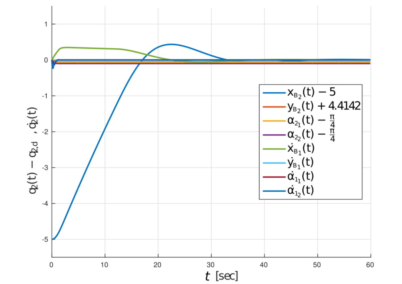
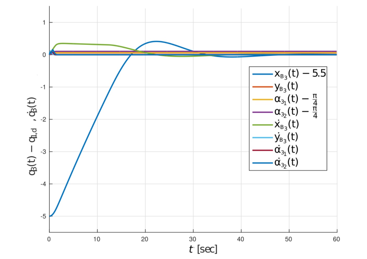
4 Rolling Contacts
In this section we relax the assumption on the rigid grasping points. In particular, we assume that the robotic agents are connected to the object in terms of rolling contacts. As discussed before, this more natural approach to cooperative manipulation allows for a wider class of objects to be manipulated, and allows for modular manipulation scenarios where robots can be swapped to adjust the grasp online.

4.1 System Model
We provide here the model of the coupled system, which is slightly different with respect to that of Section 3.1 to account for the rolling contact constraints. As before, we consider robotic agents grasping a rigid object in D space, with generalized variables . We relax the assumption of fully actuated agents by requiring , . Each agent has a smooth, convex “fingertip” (i.e. passive end-effector) of high stiffness that is in contact with an object via a smooth contact surface. In addition to the end-effector frames , we add the contact frames , located at , with respect to the inertial frame; are defined as Gauss frames [117], where one of the axes is defined orthonormal to the contact plane. We further define , . A visual representation of the contact geometry for the th agent is shown in Fig. 24. The dynamics of the th agent is given by [117]
| (69) |
with the dynamics terms as in (1), is the contact force in three dimensions, and is the Jacobian matrix to the contact point, defined by
where is the manipulator Jacobian that maps , defined in the previous section. Note the difference of (3) and (69) due to the presence of the rolling contacts. Note also that disturbances are not taken into account here for simplicity.
The full hand Jacobian matrix is , with . As before, we consider that the dynamical parameters (masses, moments of inertia) appearing in the terms , , are unknown, . The dynamics (69) can be written in vector form as
| (70) |
where , , , ⊤ , . With a slight abuse of notation, we assume that the set () contains the configurations () that yield a non-singular (in contrast to just () of the case of rigid contacts)
A common assumption in the majority of the related literature is that the object center of mass is accurately known, which is typically not the case in practice. We assume here tracking of a traceable point on the object surface instead of the center of mass , whose information is considered unknown. Note that appropriate sensor equipment, e.g., cameras and markers, can accurately track such points in practice. Hence, to remove the dependency on an unknown object center of mass, we perform a standard rigid body transformation to the conventional object dynamics as follows. Let be the respective rotation matrix of a frame attached to , and , denote the pose and generalized velocity of the object frame, with (without loss of generality) , , and . The position vector from to the respective contact point is , . Moreover, define , , and , .
Given the rolling contacts, the conventional object dynamics with respect to the object center of mass are given by the Newton-Euler formulation:
| (71) |
with the dynamic terms as in (5), and is the grasp map, defined by where , with
Note the difference of with respect to the rigid contact-case (10). We now perform a transformation of the aforementioned dynamics to account for . Let be defined as:
| (72) |
where , such that . Note that is constant.
Substitution of and left multiplication by in (71) yields the adjusted object dynamics with respect to :
| (73) |
where
with , and
Note that does not depend on . Note also by the relation , that , , are functions of , with dependency on the constant but unknown term . We also note the following relation that will be needed subsequently:
| (74) |
Similarly to the agents, the object dynamic parameters appearing in the terms , , are considered to be unknown.
The more practical consideration of rolling contacts, as opposed to a rigid grasp, requires no slip to occur between the agents and object by ensuring that each contact force remains inside the friction cone defined by:
| (75) |
where is the th contact force written in frame , whose orientation is described by , , ( being the respective Euler-angle orientation), with tangential force components and normal force component , is the friction coefficient. The full friction cone is the Cartesian product of all the friction cones: .
In practice, it is common to approximate the friction cone by an inscribed pyramid with sides. The set associated with this pyramid is defined as
| (76) |
where . The overall friction pyramid is then , where , and .
When the contact points do not slip, the grasp relation holds [98], which, after substituting (74), becomes:
| (77) |
where is the vector of contact velocities.
As in Section 3.3, we use for the object orientation the unit quaternion choice . Let hence now a desired pose trajectory, , , to be tracked by . To that end, similar to Section 3.3, we define the position error as well as the quaternion product . The aim is then to regulate to zero and to . Moreover, we aim at ensuring that the agents are always in contact with the object and slipping is avoided. Formally, the problem is defined as follows.
Problem 2.3.
In order to solve the aforementioned problem the following assumptions are made for the grasp:
Assumption 2.10.
The grasp consists of agents with non-collinear contact points and .
Assumption 2.11.
The matrix is non-singular, and the contact points do not exceed the fingertip surface.
Remark 2.9.
Note that agents with non-collinear contact points ensures is full row rank [117]. The condition that ensures the existence of a contact force that lies within the friction cone and yields a desired object wrench, which is called the force-closure condition [98]. Force-closure depends on the initial grasp, and can be ensured by existing high-level grasp planning methods [118]. Moreover, by incorporating optimization techniques, as e.g. in [119], we can enforce prevention of excessive rolling of the contacts and thus relax the respective part of Assumption 2.11. Finally, the non-singular condition of intuitively implies that tracking the desired reference trajectory does not force the agents through such singular configurations (such an assumption was also considered in the case of rigid grasps). This can also be achieved by exploiting internal motions of redundant agents ().
We also assume that the contact vectors and their derivatives are measured accurately online, . This can be achieved either by the use of appropriate tactile sensors or forward simulation of the contact dynamics [117]. By also assuming the geometry of the fingertips known, we can also compute and hence online, . Finally, note that are positive definite, and are skew-symmetric, , similarly to , and .
In the following, we present two adaptive control schemes for the solution of Problem 2.3, a centralized one, where one computer unit (or a “leader” agent) computes the input commands for the entire team, as well as a decentralized one, based on event-triggered inter-agent communication.
4.2 Centralized Scheme
This section presents the centralized proposed control scheme, which employs adaptive control techniques for the compensation of the dynamic uncertainties of the agent and object present in the problem setup.
Without loss of generality, we assume that , , i.e., the agents are not redundant. The proposed solution can be trivially extended to redundant cases, e.g., by following the analysis of [117, Chapter 6]. By combining the agent and object dynamics (70), (73) as well as (77), we can obtain the coupled dynamics
| (78) |
where
and . The following lemma states useful properties of (78):
Lemma 2.2.
The matrix is symmetric and positive-definite, and the matrix is skew-symmetric.
Proof.
The proof is similar to the one of Lemma 2.1 and is omitted. ∎
Next, we proceed to parameterizing the dynamics with respect to constant but unknown dynamic parameters, similarly to the case of rigid contacts. In particular, the left-hand side of the object dynamics (with respect to ) is parameterized as:
where , , is a vector containing the unknown object dynamic parameters, similarly to defined in Section 3.3, but also including the term , introduced in (72), and is the respective (known) regressor matrix. Similarly, the part of (78) that concerns the robotic agents can be linearly parameterized as:
with , being agent ’s regressor matrix, and , the respective vector of unknown, constant parameters. The aforementioned parameterization is written in vector form:
where , and .
Therefore, the left-hand side of the coupled dynamics (78) can be written as
| (79) |
Let now , , be the estimates of and , respectively, by the agents, and the respective errors , and .
We provide next the proposed control protocol. First, we design the reference velocity signal and the associated velocity error as
| (80a) | ||||
| (80b) | ||||
where is the positive definite gain matrix used in (21),, and . Note the difference in the definition of and from (21), which will account tot stabilizing the scalar quaternion error to either or , depending on , while guaranteeing that , (provided that ), and rendering thus (80a) well defined.
We design now the control protocol as , with
| (81) |
where , , , is the Moore-Penrose pseudoinverse of , with the positive definite gain matrix used in (23), , , and is a term in the nullspace of to prevent contact slip, which will be designed later. Moreover, we design the adaptation signals
| (82a) | ||||
| (82b) | ||||
where are constant positive definite gain matrices (as in (25)), and is the projection operator, which satisfies [110]:
| (83) |
for any symmetric positive definite , and , for some . Moreover, by appropriately choosing the initial conditions of the estimates , , we guarantee via the projection operator that , will stay uniformly bounded in predefined sets defined by finite constants , , i.e., , , . Hence, we can achieve the boundedness of the respective errors as
| (84a) | ||||
| (84b) | ||||
More details can be found in [110, Chapter 11].
We design next the internal force component to guarantee slip prevention. Slip is addressed by ensuring the contact forces remain inside the friction cone as specified in (75). From (76), we have to guarantee that , or in vector form,
| (85) |
where .
The design of the internal force component, , to ensure (85) is performed as follows. First, must be in the nullspace of , i.e., . Second, the internal force must satisfy (85). Third, the normal component of the internal force with respect to the contact plane must always be positive (i.e. the manipulators cannot ‘‘pull” on the contact point). To enforce this condition we design11 1 We use the notation . , where is the internal force direction in the contact frame , , and is a gain parameter to be designed. Without loss of generality let be aligned with the normal direction of the contact frame such that , , ensures that only pushing forces are applied at each contact. Satisfaction of the aforementioned conditions is done by solving the following convex quadratic program to define the internal force controller
| (86a) | ||||
| (86b) | ||||
| s. t. | (86c) | |||
| (86d) | ||||
| (86e) | ||||
| (86f) | ||||
where . Note that, since the contact points form a force-closure configuration, (86) always has a feasible solution.
Finally, to satisfy (85), must apply sufficient force inside the friction cone to reject perturbations that will arise during the manipulation motion that can push the contact force outside of the friction cone. Rejection of these perturbations is performed by designing the gain as follows. For simplicity we define the terms , and we denote by and the th scalar element of and respectively for .
Noting that from (86), we define the decreasing function as
where , , is an appropriate polynomial that ensures continuous differentiability of , for instance . Then one can verify that , . We now design the magnitude scaling for the internal forces as
| (87) |
where is a tuning gain. The intuition behind (87) is to upper bound elements of the control and the system dynamics to prevent either from pushing the contact force outside of the friction cone. The term cancels out any effects from . The term handles the system dynamics, which is guaranteed to be bounded in the following theorem.
Remark 2.10.
The internal force control presented here accounts for the dynamics of the system by appropriately scaling , which rejects perturbations from causing slip. However, as opposed to [120], we relax the condition that must upper bound all of the dynamics terms by exploiting knowledge of the applied controller via the term . This reduces the amount of squeezing force applied to prevent crushing the object.
The stability and slip prevention guarantees of the proposed controller are presented in the following theorem.
Theorem 2.5.
Consider robotic agents in contact with an object, described by the dynamics (70), (73), and suppose Assumptions 2.10 and 2.11 hold. a the desired object pose be bounded with bounded first and second derivatives. Moreover, assume that and , . Then, the control protocol (80a)-(87) guarantees that , as well as boundedness of all closed-loop signals. Moreover, by choosing a sufficiently large in (87), it holds that , .
Proof.
Consider the stack vector state . Next, note by (70), (71), and (77) that, when , each can be written as a function of the stack state, i.e., , . Consider also the set
for some positive constants , , satisfying , , , and larger than , respectively, which were introduced in (84). Note that . Next, by using (81) and (82), one obtains the closed-loop dynamics , where is a function that is continuous in and locally Lipschitz in . Then, according to Theorem 8.1 of Appendix 8, there exists a positive time constant and a unique solution , i.e., defined for and satisfying , . Hence, slip is prevented and the dynamics (78) are well-defined, for .
Let now the Lyapunov function
| (88) |
Since , it holds that for a finite positive . Differentiation of results in:
Exploitation of the skew symmetry of , use of , use of (79), and substitution of the control law (81) results in:
where we used the fact that through (86). Finally, by substituting the adaptation laws (82), we obtain
which, by invoking the projection operator property (83) becomes . Thus is negative semi-definite, and is bounded in a compact set as , . In addition, , . Hence, the terms , , are bounded in a compact set defined by and not dependent on , . Therefore, since and are bounded and have bounded derivatives, one concludes that , , and , are also bounded in compact sets, . This also implies boundedness of , as introduced in (78), which, along with Assumption 2.11 and properties of Euler-Lagrange systems [121], implies that , , , are also bounded in compact sets that are independent of , . We prove next the slip prevention using the design of the internal force component . By using (70), (73) and (77), one obtains the following expression for the interaction forces:
| (89) |
where , which, by replacing , using and (79), adding and subtracting and adding , becomes
| (90) |
where
By combining the aforementioned expression with (85), one obtains the following condition for slip prevention:
| (91) |
Note that due to the aforementioned Lyapunov analysis, as well as the adaptation laws (82) through the projection operator, , , , , are bounded in compact set independent of , . By combining this with the aforementioned analysis, we conclude that is bounded for all in a compact set, independent of . Hence, by denoting the maximum bound of the elements of and using the designed internal force component , a sufficient condition for (91) to hold is for the th element to satisfy
. By substituting (87), the left side satisfies
where we use , , , and , , since is decreasing. Hence, by choosing a large enough we guarantee and hence contact slip is avoided . In fact, the internal forces analysis above and the fact that defines pyramid constraints imply that , where is a compact subset of , . Therefore, since and are uniformly bounded through the projection operator by and , respectively, by choosing large enough , , and in the definition of , belongs to a compact subset of , . Thus by invoking Theorem 8.2 of Appendix 8, it follows that .
Note, finally, that , as designed in (81), is bounded, . Therefore, one can conclude that and thus is bounded, . Hence, it follows that is also bounded, . Thus by invoking Barbalat’s lemma (Lemma 8.1 of Appendix 8), it follows that and so and . This implies that , which, given that is a unit quaternion and , , ensures asymptotic stability of the pose error as .
∎
Remark 2.11.
Note that the bound of in (90) can be computed a priori. In practice, the terms , , which concern masses and moments of inertia of the object and the agents, can be known a priori up to a certain accuracy, leading thus to respective bounds. Hence, one can compute upper bounds for and hence for , , , and . Since the structure of the dynamic terms is known, this can also lead to a bound of the terms , , , , , , and that appear in . Hence, tuning of to overcome can be performed off-line.
4.2.1 Simulation Results
The proposed control algorithm ensures asymptotic stability for cooperative manipulation with rolling contacts, as well as no slip, while being robust to dynamic uncertainties of the object-robot system. In this section, we implement the proposed control scheme on three 6 DoF mobile manipulators consisting of a 3 DoF, kg base (X-Y translation, rotation about Z) and a 3-DoF manipulator with identical links of length m and mass of kg each, as depicted in Fig. 25. The objective is to transport a kg box along the desired reference trajectory defined by m, . The control gains used are: , , , , , . The control is implemented with 30% error in all uncertain parameter (including the object center of mass), and the projection operator enforces the following bounds on the uncertain terms: , .
The simulation results are depicted in Figs. 26-30 for seconds. More specifically, Figs. 26 and 27 show the resulting error trajectories of the object-agent system, which satisfy , , and in the presence of rolling effects. Fig. 28 illustrates the boundedness of the uncertain parameters, that is enforced by the proposed control scheme. Fig. 29 shows the required friction, , which denotes the minimum friction coefficient necessary to prevent slip throughout the motion [120]. If the required friction surpasses the true coefficient, then the contact point will slip and the grasp is compromised. As shown in Fig. 29, however, the required friction for each contact is below the true coefficient of , which indicates that slip is prevented as guaranteed by the proposed method. Finally, Fig. 30 depicts the control inputs of the agents. As predicted by the theoretical analysis, asymptotic error stability as well as contact slip prevention are achieved.


4.3 Decentralized Scheme
This section presents a decentralized extension of the aforementioned scheme via event-triggered communication among the agents. The event-triggered control requires an update law (to be designed) that updates relevant variables at each time for . We use the subscript with to denote a variable that is held constant over the time interval and updated at each . The variables communicated among the agents at time are and , allowing all the agents to reconstruct , as well as , with , , . The event-triggered manipulation control law is defined as:
| (92a) | ||||
| (92b) | ||||
with , with the decentralized version of the adaptive update laws defined by (82):
| (93a) | ||||
| (93b) | ||||
where , is such that from (82), and is the event-triggered internal force control yet to be designed. Similarly, is a generalized inverse of the grasp map at and we denote . Let , , , denote the triggering errors. Note that (92) is only dependent on the full grasp map, , in the term , whereas the adaptation laws (93) and remainder of the control depend on .
Moreover, in order to ensure no slip, recall that the condition (85) must hold. Notice that when there is no communication between agents, and are unknown as each agent only has knowledge of and . Thus if the original internal force control (86) is implemented with , the errors and may induce slip. To account for this, we use a conservative that effectively shrinks the friction pyramid. The design of is dependent on the allowable error that will result from triggering. This presents a trade-off where to reduce communication (i.e reduced triggering), a smaller more conservative is required, and vice versa (i.e. larger requires more communication between agents). We introduce the following Lemma to compute .
Lemma 2.3.
Let , and satisfying , where is a positive constant satisfying
| (94) |
and define
| (95) |
If satisfies , then .
Proof.
Denote by the angle defined by and , satisfying
| (96) |
where . Note that and hence has strictly positive eigenvalues, rendering positive and .
Moreover, it holds as well as . Hence, by taking into account and (94), (96) becomes
implying
| (97) |
and rendering hence positive.
In order for to belong to , must lie in a new friction cone , whose angle must be reduced by from , leading thus to . In view of (97), it holds that and hence and . ∎
The event-triggered internal force controller is now defined as follows:
| (98a) |
| (98b) | ||||
| s. t. | (98c) | |||
| (98d) | ||||
| (98e) |
| (99) |
where , , is the th agent’s part in vector , and are the th scalar elements of , and , respectively, are design parameters, and is defined as in (95). Note that is constant for such that it need only be computed at each update.
Now that the full control protocol is defined, the final step is to define the event-triggering condition to update and which are:
| (100a) | ||||
| (100b) | ||||
| (100c) | ||||
| (100e) | ||||
where is the th component of , , , , , , , are design parameters. Note that due to the fact that is full row rank. The time for which an event is triggered is when (100a), (), or (100e) are satisfied, and formally defined as:
| (101) |
Note that the condition (101) can be evaluated by each agent individually. When one agent identifies a triggering condition, the agent then signals to all agents that an update is required and all agents then only communicate and for all .
The proposed control is decentralized with aperiodic updates of only each agent’s contact information. The event-triggered, decentralized control law ensures practical asymptotic stability of the origin as presented in the following theorem:
Theorem 2.6.
Consider robotic agents in contact with an object, described by the dynamics (70), (73), and suppose Assumptions 2.10 and 2.11 hold. Let the desired object pose be bounded with bounded first and second derivatives. Moreover, assume that and , . Then, by choosing sufficiently large control gains , , , the event-triggered control protocol (92), (93), (98) with event-triggered mechanism (101) guarantees ultimate boundedness of , in a set around the origin, and by choosing sufficiently large , , , it holds that , .
Proof.
The proof is structured into 2 Cases. Case 1 addresses the system if no event is triggered. Case 2 addresses the triggering conditions and ensuring non-Zeno behavior for the time updates.
Case 1: Here we address the case when no event is triggered such that and . We note from the proof of Theorem 2.5 that the continuous control law, from (81) ensures asymptotic stability of the system with the Lyapunov candidate function, , defined in (88). We define the following compact set:
with as defined in (88), and .
From , the same analysis from Theorem 2.5 applies here such that there exists a such that for , slip does not occur and the solution is unique. In the following we will apply the Lyapunov analysis over the time interval .
After substitution of (92), becomes
From it follows that which yields, along with (93), (83), and the fact that :
Note that can be increased by tuning . From and , it follows that . From the triggering condition (101), it follows that for all . We thus define , which is constant between events, such that . Note that Assumptions 2.10 and 2.11 as well as the fact that slip does not occur for imply that is well defined and bounded, . Hence becomes
We then complete the squares such that and hence becomes
Now we introduce such that:
where and . By choosing large enough , , and , we can achieve and .
Let now . Note that is compact since , are bounded as per (84). Moreover, in it holds that and hence , and becomes
According to (100e), it holds, between events, that
By summing for all , the latter becomes
implying that . By following Barbalat’s Lemma, it can be shown that will enter the set in finite time.
By using (84), we now investigate inside for which it holds :
where , are positive constants. Since , it holds that , which is bounded, since , and is full row rank. Furthermore is constant between events. Thus in view of (84) and since lies in the compact set , we can conclude that there exists a such that:
Hence becomes
where . Therefore, by invoking Lemma 8.1 of Appendix 8, we guarantee that is ultimately bounded in a compact set defined by and , for .
Now we investigate the slip prevention properties, similar to that of Theorem 2.5. The same derivation of yields:
By following a similar procedure as with the previous section, we conclude that
Substitution of into (85), which ensures slip prevention, yields the following condition to be satisfied:
From the boundedness of signals, we conclude that is bounded for all in a compact set, independent of . Now let denote the maximum bound of the elements of and substitute with to re-write the sufficient condition for no slip as:
or, for each agent separately,
| (102) |
where is the th agent’s part in (as opposed to the scalar ), is th block matrix of ’s diagonal and is the -block matrix of . Here we show that the triggering conditions (100a) and (100b) ensure that . By boundedness of the system dynamics, for sufficiently large bounding the terms , it follows that . Since and it follows that , , and hence Lemma 2.3 dictates that (4.3) is satisfied when
where as given by (95).
From the boundedness of signals, there exists a such that for all . Furthermore, we know is constant between updates and known to all agents. Therefore at each update and can be computed, and we note that is bounded by Assumption 2.10. Thus a sufficient condition for the above expression to hold is:
, which is feasible since from (100b).
By substituting (99) with the choice of , the left side satisfies
where we use , , , and , , since is decreasing. Hence, by choosing a large enough we guarantee and hence contact slip is actively prevented . Following the proof of 2.5, it follows that , and thus slip prevention is ensured for the entirety of the manipulation task.
Furthermore, since , the previous Lyapunov analysis ensures that when , guaranteeing thus, in view of Lemma 8.1 of Appendix 8, that will be ultimately bounded in a compact set around the origin, rendering the closed-loop system practically asymptotically stable.
Case 2: In the previous analysis, practical asymptotic stability is ensured when no triggering occurs. Here we show that indeed the event triggering preserves the results from Case 1 and that the system does not exhibit Zeno behavior. For any , it follows that . Thus if any event triggers in at , and , and it is straightforward to see that such that . Furthermore holds after the event occurs and ensures enters in finite time.
For , the condition holds although will change between events. However, since and are bounded in , there exists a maximum for which is ultimately bounded, and practical stability is preserved.
Now we show there exists a lower bound between each event time instant. Events (100a) and () are dependent on bounds , and , where is fixed and and will never tend to zero due to boundedness of . From the continuous differentiability of and , let denote their respective Lipschitz constants. It follows that there exist lower bounds on event times defined by , , respectively.
Similarly, the event defined by (100e) depends on the bound . Denote by . Then (100e) occurs when
where , , , with . Therefore, since from (100b) and , , , are bounded in compact sets for from the previous analysis, there exist positive constants and such that and , . Hence, by taking into account (100a) it holds that , with being the inter-sampling time between the updates defined by (100e). We conclude then that .
5 Conclusion
This chapter presented novel control protocols for the cooperative manipulation of a single object by robotics agents without employing force sensing. Firstly, we focused on rigid grasps, by introducing two adaptive decentralized control schemes that used quaternion-feedback and prescribed performance control, respectively. Next, we incorporated collision avoidance by using nonlinear MPC, in a centralized and a communication-based decentralized scheme. Secondly, we considered the case of rolling contacts. We developed novel adaptive centralized and decentralized control schemes that compensate for the object’s and the agents’ dynamic uncertainties and guarantee avoidance of contact loss at the contact points.
Chapter 3 Formation Control and Rigid Cooperative Manipulation
As discussed in Chapter 1, an important problem associated with multi-agent coordination is formation control. On one hand, formation specifications can be imposed by a higher level planner associated with temporal tasks. Moreover, as we show here, a particular instance of multi-agent formations, namely rigid formation, is tightly associated to rigid cooperative manipulation presented in the previous chapter. More specifically, this chapter addresses the following two topics.
Firstly, it deals with the problem of distance- and orientation-based formation control of a class of second-order nonlinear multi-agent systems in , under static and undirected communication topologies. More specifically, we design a decentralized model-free control protocol in the sense that each agent uses only local information from its neighbors to calculate its own control signal, without incorporating any knowledge of the model nonlinearities and exogenous disturbances. Moreover, the transient and steady-state response is solely determined by certain designer-specified performance functions and is fully decoupled by the agents’ dynamic model, the control gain selection, the underlying graph topology as well as the initial conditions. Additionally, by introducing certain inter-agent distance constraints, we guarantee collision avoidance and connectivity maintenance between neighboring agents.
Secondly, we introduce a new notion of distance rigidity, namely distance- and bearing-rigidity in , and we connect it with rigid cooperative manipulation. More specifically, the nodes of a general rigid framework are associated to the robotic agents of rigid cooperative manipulation schemes and the object-agent interaction forces are expressed by using the rigidity matrix of the graph formed by the robots, which encodes the infinitesimal rigid body motions of the system. Moreover, we show that the associated cooperative manipulation grasp matrix is related to the rigidity matrix via a range-nullspace relation, based on which we provide novel results on the relation between the arising interaction and internal forces and consequently on the energy-optimal force distribution on a cooperative manipulation system.
6 Introduction
During the last decades, decentralized control of networked multi-agent systems has gained a significant amount of attention due to the great variety of its applications, including multi-robot systems, transportation, multi-point surveillance and biological systems. The main focus of multi-agent systems is the design of distributed control protocols in order to achieve global tasks, such as consensus [122, 2, 3, 4], and at the same time fulfill certain properties, e.g., network connectivity [6, 10].
A particular multi-agent problem that has been considered in the literature is the formation control problem, where the agents represent robots that aim to form a prescribed geometrical shape, specified by a certain set of desired relative configurations between the agents. The main categories of formation control that have been studied in the related literature are ([7]) position-based control, displacement-based control, distance-based control and orientation-based control.
In distance-based formation control, inter-agent distances are actively controlled to achieve a desired formation, dictated by desired inter-agent distances. Each agent is assumed to be able to sense the position of its neighboring agents. When orientation alignment is considered as a control design goal, the problem is known as orientation-based (or bearing-based) formation control. The orientation-based control steers the agents to configurations that achieve desired relative orientation angles. In this work, we aim to design a decentralized control protocol such that both distance- and orientation-based formation is achieved.
The literature in distance-based formation control is rich, and is traditionally categorized in single or double integrator agent dynamics and directed or undirected communication topologies (see e.g. [7, 123, 124, 125, 126, 127, 128, 129, 130, 131, 132, 133, 134, 135, 136, 137, 138]). Orientation-based formation control has been addressed in [139, 140, 141, 142], whereas the authors in [141, 143, 144] have considered the combination of distance- and orientation-based formation.
In most of the aforementioned works in formation control, the two-dimensional case with simple dynamics and point-mass agents has been dominantly considered. In real applications, however, the engineering systems have nonlinear second order dynamics and are usually subject to exogenous disturbances and modeling errors. Other important issues concern the connectivity maintenance, the collision avoidance between the agents and the transient and steady-state response of the closed loop system, which have not been taken into account in the majority of related woks. Thus, taking all the above into consideration, the design of robust distributed control schemes for the multi-agent formation control problem becomes a challenging task.
Another special instance of formation control that has practical relevance and numerous applications in robotics is that of rigid formations. Two cases of rigid formation control have been widely studied in the literature, namely distance rigidity and bearing rigidity. The classic distance rigidity theory studies the problem of under what conditions can the geometric pattern of a network be uniquely determined if the length (distance) of each edge in the multi-agent team is fixed. It is a combinatorial theory for characterizing the “stiffness” or “flexibility” of structures formed by rigid bodies connected by flexible linkages or hinges, and it has been applied extensively in distance-based formation control and network localization [145, 146, 147, 148, 149, 150, 151, 152, 153, 154, 155, 156]. Bearing rigidity theory studies the fundamental problem of under what conditions can the geometric pattern of a multi-agent system be uniquely determined if the bearing of each edge is fixed [157], and it has been used for bearing-based control and estimation problems [158, 159, 160, 161]. Recent works have developed bearing rigidity theory on the manifolds of [162] and [163]. In this chapter, we introduce the notion of distance and bearing rigidity, which studies under what conditions can the geometric pattern of a multi-agent system be uniquely determined if both the distance and the bearing of each edge is fixed. Moreover, we combine the latter with rigid cooperative manipulation, i.e., configurations where a number of robotic agents are attached to a common object by means of rigid contact points.
As shown in the previous chapter, rigid cooperative manipulation by robotic agents (i.e., when the grasps are rigid) is an important and challenging topic, indispensable in cases of difficult maneuvers or heavy payloads. An important property in rigid cooperative manipulation systems that has been studied thoroughly in the related literature and overlooked in the previous chapter, is the regulation of internal forces. Internal forces are forces exerted by the agents at the grasping points that do not contribute to the motion of the object. While a certain amount of such forces is required in many cases (e.g., to avoid contact loss in multi-fingered manipulation), they need to be minimized in order to prevent object damage and unnecessary effort of the agents. Most works in rigid cooperative manipulation assume a certain decomposition of the interaction forces in motion-inducing and internal ones, without explicitly showing that the actual internal forces will be indeed regulated to the desired ones (e.g., [59, 54, 52]); [164, 165, 166, 73] analyze specific load decompositions based on whether they provide internal force-free expressions, whereas [69] is concerned with the cooperative manipulation interaction dynamics. The decompositions in the aforementioned works, however, are based on the inter-agent distances and do not take into account the actual dynamics of the agents. The latter, as we show in this chapter, is tightly connected to the internal forces as well as their relation to the total force exerted by the agents at the grasping points.
This chapter deals with the following two topics:
- 1.
Firstly, we address the distance-based formation control problem with orientation alignment for a team of rigid bodies operating in , with unknown second-order nonlinear dynamics and external disturbances. We propose a purely decentralized control protocol that guarantees distance formation, orientation alignment as well as collision avoidance and connectivity maintenance between neighboring agents and in parallel ensures the satisfaction of prescribed transient and steady state performance. The prescribed performance control framework has been incorporated in multi-agent systems in [167] and [168] for minimally rigid formations, where first order dynamics have been considered without taking into account the problem of orientation alignment.
- 2.
We integrate rigid cooperative manipulation with rigidity theory. Motivated by rigid cooperative manipulation systems, where the inter-agent distances and bearings are fixed, we introduce the notion of distance and bearing rigidity in the special Euclidean group . Based on recent results, we show next that the interaction forces in a rigid cooperative manipulation system depend on the distance and bearing rigidity matrix, a matrix that encodes the allowed coordinated motions of the multi-agent-object system. Moreover, we prove that the cooperative manipulation grasp matrix, which relates the object and agent velocities, is connected via a range-nullspace relation to the rigidity matrix. Furthermore, we rely on the aforementioned findings to provide new results on the internal force-based rigid cooperative manipulation. We derive novel results on the relation between the arising interaction and internal forces in a cooperative manipulation system. This leads to novel conditions on the internal force-free object-agents force distribution and consequently to optimal, in terms of energy resources, cooperative manipulation.
Finally, we verify all the theoretical findings through simulation results.
7 Formation Control in
7.1 Problem Formulation
Consider a set of rigid bodies, with , , operating in a workspace . We consider that each agent occupies a ball , where is the position of the agent’s center of mass with respect to an inertial frame and is the agent’s radius (see Fig. 31). We also denote by the rotation matrix associated with the orientation of the th rigid body. Moreover, we denote by and the linear and angular velocity of agent with respect to frame . The vectors are expressed in coordinates, whereas and are expressed in a local frame centered at each agent’s center of mass. The position, though, of , is not required to be known by the agents, as will be shown later. By defining and , we model each agent’s motion with the nd order Newton-Euler dynamics:
| (103a) | ||||
| (103b) | ||||
where the matrix is the constant positive definite inertia matrix, is the Coriolis matrix, is the body-frame gravity vector, is a bounded vector representing model uncertainties and external disturbances, and , where is the tangent space to at . Finally, is the control input vector representing the D generalized force acting on agent . The following properties hold for the aforementioned terms:
- •
The terms are unknown, are continuous and it holds that
(104a) (104b) , where is a finite unknown positive constant and , and , which are also uknown, .
- •
The functions are assumed to be continuous in and for each fixed , the functions are assumed to be bounded by unknown positive finite constants , i.e., , , .
It is also further assumed that each agent has a limited sensing range of . Therefore, by defining the set , with , and , agent can measure the relative offset (i.e., expressed in ’s local frame), the distance , as well as the relative orientation with respect to its neighbors . In addition, we consider that each agent can measure its own velocity subject to time- and state-varying bounded noise, i.e., agent has continuous feedback of , , where are vector fields bounded by unknown positive finite constants , i.e., , , . Moreover, the vector fields with are assumed to be continuous in and for each fixed , the functions are assumed to be bounded by unknown positive finite constants , i.e., , , .
Remark 3.1.
(Local relative feedback) Note that the agents do not need to have information of any common global inertial frame. The feedback they obtain is relative with respect to their neighboring agents (expressed in their local frames) and they are not required to perform transformations in order to obtain absolute positions/orientations. In the same vein, note also that the velocities are vectors expressed in the agents’ local frames.
The topology of the multi-agent network is modeled through the undirected graph , with (i.e., the initially connected agents), which is assumed to be nonempty and connected. We further denote where . Given the -th edge, we use the simplified notation for the function that assigns to edge the respective agents, with , . Since the agents are heterogeneous with respect to their sensing capabilities (different sensing radii ), the fact that the initial graph is nonempty, connected and undirected implies that
with . We also consider that is static in the sense that no edges are added to the graph. We do not exclude, however, edge removal through connectivity losses between initially neighboring agents, which we guarantee to avoid. That is, the proposed methodology guarantees that , , . It is also assumed that at the neighboring agents are at a collision-free configuration, i.e., , with . Hence, we conclude that
| (106) |
The desired formation is specified by the constants , for which, the formation configuration is called feasible if the set is nonempty. Due to the fact that the agents are not dimensionless and their communication capabilities are limited, the control protocol, except from achieving a desired inter-agent formation and maintaining connectivity, should also guarantee for all that the initially neighboring agents avoid collision with each other. Therefore, all pairs of agents that initially form an edge must remain within distance greater than and less than . We also make the following assumptions that on the graph topology:
Assumption 3.1.
The communication graph is a tree.
Formally, the robust formation control problem under the aforementioned constraints is formulated as follows:
Problem 3.1.
The term “robust” here refers to robustness of the proposed methodology with respect to the unknown dynamics and external disturbances in (103) as well as the unknown noise in the velocity feedback.
7.2 Problem Solution
Let us first introduce the distance and orientation errors:
| (107a) | ||||
| (107b) | ||||
, where we have used Proposition 14.3 of Appendix 14. Regarding , our goal is to guarantee from all initial conditions satisfying (106), while avoiding inter-agent collisions and connectivity losses among the initially connected agents specified by . Regarding , we aim to guarantee the following:
- 1.
- 2.
By using the properties of skew-symmetric matrices presented Appendix 14, we derive the following dynamics of the errors (107):
| (108a) | ||||
| (108b) | ||||
where and , .
By employing Proposition 14.2 of Appendix 14, we obtain as well as
Hence, it holds that:
| (109) |
which implies that: , . The two configurations and correspond to the desired and undesired equilibrium, respectively.
The concepts and techniques of prescribed performance control (see Appendix 9) are adapted in this work in order to: a) achieve predefined transient and steady-state response for the distance and orientation errors , , , as well as ii) avoid the violation of the collision and connectivity constraints between initially neighboring agents, as presented in Section 7.1. The mathematical expressions of prescribed performance are given by the inequality objectives:
| (110a) | ||||
| (110b) | ||||
, where , , with
are designer-specified, smooth, bounded, and decreasing functions of time; the constants , , and , , , incorporate the desired transient and steady-state performance specifications respectively, as presented in Section 9, and , , are associated with the collision and connectivity constraints. In particular, we select
| (111a) | ||||
| (111b) | ||||
, which, since the desired formation is compatible with the collision and connectivity constraints (i.e., ), ensures that , and consequently, in view of (106), that:
| (112a) | |||
| . Moreover, assuming that , , by choosing | |||
| (112b) | |||
| it is also guaranteed that: | |||
| (112c) | |||
. Hence, if we guarantee prescribed performance via (110), by setting the steady-state constants arbitrarily close to zero and by employing the decreasing property of , we guarantee practical convergence of the errors to zero and we further obtain:
| (113a) | ||||
| (113b) | ||||
, which, owing to (111), implies:
, providing, therefore, a solution to problem 3.1. Moreover, note that the choice of along with (113) guarantee that , and the avoidance of the singular equilibrium.
In the sequel, we propose a decentralized control protocol that does not incorporate any information on the agents’ dynamic model and guarantees (110) for all .
Given the errors defined in the previous section, we perform the following steps:
Step I-a: Select the corresponding functions and positive parameters , , , following (110), (112b), and (111), respectively, in order to incorporate the desired transient and steady-state performance specifications as well as the collision and connectivity constraints, and define the normalized errors, ,
| (114) |
Step I-b: Define the transformations , , and by
, and the transformed error states , , ,
| (115a) | ||||
| (115b) | ||||
Next, we design the decentralized reference velocity vector for each agent as
| (116) |
where are positive gains, , with , , and the function is defined as , if is the tail of the th edge (), if is the head of the th edge (), and otherwise (see Appendix 12 for more details on graph edges). The assignment of the head and tail in each edge can be done off-line according to the specified orientation of the graph.
Step II-a: Define for each agent the velocity errors , , and design the decreasing performance functions as , with , where the constants incorporate the desired transient and steady-state specifications, with the design constraints , , , . The term can be measured be each agent at directly after the calculation of .
Moreover, define the normalized velocity errors
| (117) |
where , .
Step II-b: Define the transformation as
and the transformed error states as
| (118) |
Finally, design the decentralized control protocol for each agent as , with
| (119) |
where with , , and are positive gains, .
Remark 3.2.
(Control protocol intuition) Note that the selection of according to (111) and of such that along with (106), guarantee that , , , , , . The prescribed performance control technique enforces these normalized errors and to remain strictly within the sets , and , respectively, , guaranteeing thus a solution to Problem 3.1. It can be verified that this can be achieved by maintaining the boundedness of the modulated errors and in a compact set, .
Remark 3.3.
(Arbitrarily fast convergence to ) The configurations where or are equilibrium configurations that result in , . If , which is a local minima, the orientation formation specification for edge cannot be met, since the system becomes uncontrollable. This is an inherent property of stabilization in , and cannot be resolved with a purely continuous controller [113]. Moreover, initial configurations starting arbitrarily close to might take infinitely long to be stabilized at with common continuous methodologies [114]. Note however, that the proposed control law guarantees convergence to arbitrarily fast, given that . More specifically, given the initial configuration , we can always choose such that , regardless of how close is to . Then, as proved in the next section, the proposed control algorithm guarantees (110b) and the transient and steady-state performance of the evolution is determined solely by and more specifically, the rate of convergence is determined by the term . It can be observed from the desired angular velocities designed in (116) that close to the configuration , the term , which is close to zero (since ), is compensated by the term , which attains large values (since is close to 1). Moreover, potentially large values (but always bounded, as proved in the next section) for and hence due to the term can be compensated by tuning the control gains and .
Remark 3.4.
(Decentralized manner, relative feedback, and robustness) Notice by (116) and (119) that the proposed control protocols are distributed in the sense that each agent uses only local relative information to calculate its own signal. In that respect, regarding every edge , the parameters , as well as the sensing radii , which are needed for the calculation of the performance functions , can be transmitted off-line to the agents . In the same vein, regarding , i.e., the constants can be transmitted off-line to each agent , which can also compute , given the initial velocity errors . Notice also from (116) that each agent uses only relative feedback with respect to its neighbors. In particular, for the calculation of , the tail of edge , i.e., agent , uses feedback of , and the head of edge , i.e., agent , uses feedback of . Both of these terms are the relative inter-agent position difference expressed in the agents’ local frames. For the calculation of , agents and require feedback of the relative orientation , as well as the signal , which is a function of . The aforementioned signals encode information related to the relative pose of each agent with respect to its neighbors, without the need for knowledge of a common global inertial frame. It should also be noted that the proposed control protocol (119) depends exclusively on the velocity of each agent and not on the velocity (expressed in a local frame) of its neighbors. Moreover, the proposed control law does not incorporate any prior knowledge of the model nonlinearities/disturbances, enhancing thus its robustness. Finally, the proposed methodology results in a low complexity. Notice that no hard calculations (neither analytic nor numerical) are required to output the proposed control signal.
We provide now the main result of this section0, which is summarized in the following theorem.
Theorem 3.1.
Consider the multi-agent system described by the dynamics (105), under a static tree communication graph , aiming at establishing a formation described by the desired offsets and , . Then, the control protocol (114)-(119) guarantees the prescribed transient and steady-state performance
, , under all initial conditions satisfying , and (106), providing thus a solution to Problem 3.1.
Proof.
We start by defining some vector and matrix forms of the introduced signals and functions:
where .
With the introduced notation, (108) can be written in vector form as:
| (120a) | ||||
| (120b) | ||||
where ,
is the orientation incidence matrix of the graph:
| (121) |
with , and is the incidence matrix of the graph (see Section 12.A of Appendix 12). The terms and in correspond to the block diagonal matrix with the agents’ rotation matrices along the main block diagonal, and the block diagonal matrix with the rotation matrix of each edge’s tail along the main block diagonal, respectively. These two terms have motivated the incorporation of the terms in the desired velocities designed in (116), since, as shown next, the vector form yields the orientation incidence matrix .
The desired velocities (116) and control inputs (119) can be written in vector form as
| (122a) | ||||
| (122b) | ||||
| (122c) | ||||
where and . Note from (122c) and (114), (117), (115), (118) that can be expressed as a function of the states . Hence, the closed loop system can be written as
By defining , we can write the closed loop system in vector form as
| (123) |
Next, define the set
where we abuse the notation and express , , from (114), (117) as a function of the states. It can be verified that the set is open due to the continuity of the operators and nonempty, due to (111). Our goal here is to prove first that (123) has a unique and maximal solution in and then that this solution stays in a compact subset of .
It can be verified that the function is (a) continuous in for each fixed , and (b) continuous and locally lipschitz in for each fixed . Therefore, the conditions of Theorem 8.1 of Appendix 8 are satisfied and hence, we conclude the existence of a unique and maximal solution of (123) for a timed interval , with , such that , . This implies that
| (124a) | ||||
| (124b) | ||||
| (124c) | ||||
, , . Therefore, the signals are bounded for all . In the following, we aim to show that the solution is bounded in a compact subset of and hence, by employing Theorem 8.2 of Appendix 8, that .
Consider the positive definite Lyapunov candidate , with , which is well defined for , due to (124a). By differentiating and taking into account the dynamics , we obtain
which, by substituting and (120), becomes
| (125) |
where (by employing (121)), and , are the linear parts of and (i.e., the stack vector of the first three components of every , ), respectively. Note first that, due to (124c), the function is bounded for all . Moreover, note that (124a) implies that , . Therefore, it holds that , . In addition, since is a connected tree graph and , , is positive definite (see Lemma 12.1 of Appendix 12) and hence . Hence, we conclude that and the positive definiteness of , . In addition, since , we also conclude that the term is upper bounded, . Finally, and are bounded by definition and assumption, respectively, . Note that all the aforementioned bounds are independent of . We obtain now from (125):
where
and is a positive constant, independent of , satisfying the following inequality: . Note that, in view of the aforementioned discussion, is finite.
Hence, we conclude that . By noting that
, as well as , , we conclude that , , where . Hence, we conclude that , , and therefore
| (126) |
, and by taking the inverse logarithm function:
| (127) |
, where , and . Hence, (126) and (127) imply the boundedness of , , , and in compact sets, , and therefore, through (116), the boundedness of , , .
Similarly, consider the positive definite Lyapunov candidate , with . By differentiating and taking into account the dynamics , we obtain
which, after substituting (108b), (120), becomes
where and are the angular parts of and (i.e., the stack vector of the last three components of every , ), respectively. By substituting (122b) and defining , , we obtain:
| (128) |
According to (121), . Since and are rotation (and thus unitary) matrices, the singular values of are identical to the ones of , and hence . Indeed, let be a singular value decomposition of , where , are unitary matrices, and is a diagonal matrix containing the singular values of . Then where , and are unitary matrices (being products of unitary matrices). Thus, is the singular value decomposition of , and hence its singular values are the diagonal values of . By further defining , with , , (128) becomes
Note that, by construction, , , and . Hence, in view of (124b), we conclude that , . By noting also that , becomes
where is a positive constant, independent of , satisfying , . Note that is finite, , due to (124b) and the boundedness of the noise signals. After substituting (109), we obtain
| (129) |
From (124b) we conclude that , and hence , . Moreover, by noticing that , , and , , (129) becomes
where
From (124b), (114), and the fact that , it holds that . By also employing the property
we obtain
where:
We conclude therefore that . From (115b), given , we obtain:
. Therefore, , and according to Proposition 14.1 of Appendix 14,
Hence, we conclude that . Therefore,
| (130) |
and, by taking the inverse logarithm:
| (131) |
where and , . Therefore, we conclude the boundedness of , in compact sets, , and therefore, through (116), the boundedness of , . From the proven boundedness of and , we also conclude the boundedness of and invoking and (124c), the boundedness of and , . Moreover, in view of (126), (127), (123), (116), we also conclude the boundedness of .
Proceeding along similar lines, we consider the positive definite Lyapunov candidate with . By computing and using the dynamics , we obtain
| (132) |
Since we have proved the boundedness of and , the terms , , and are also bounded, , due to the continuities of , , and in , and the boundedness of and in . Moreover, , , and are also bounded due to (104b), (124c), and by construction, respectively. By also using (104a), we obtain from (132):
where is a positive finite term, independent of , satisfying , and . Hence, . By noting that
, as well as , , we conclude that , , where . Hence, we conclude that , and consequently that
and by taking the inverse logarithm function:
| (133) |
, where . Note that the term is finite, . Moreover, the term is finite due to the choice . Hence, since is strictly positive, the term is also finite. Thus, the term and hence the control laws (119) are also bounded in compact sets for all .
What remains to be shown is that . Towards that end, suppose that is finite, i.e., . Then, according to Theorem 8.2 of Appendix 8, it holds that , where is the distance of to . We first rewrite the condition in a more explicit form, in order to account for the matrix tuple . We define , the projection sets and as well as the distance from a set as with , where is the induced norm in defined as , for . Therefore, the condition of Theorem 8.2 of Appendix 8 can now be stated as follows: Since , it holds that
| (134) |
which we aim to prove that is a contradiction. Firstly, it holds that
However, according to Proposition 14.3, it holds that for any . Hence, . Moreover, from (133) and (117) we obtain , . By invoking (126), (130), we can also conclude that there exists a finite such that , . Hence, since , , implies that there exists a finite such that , . Hence, , , which proves the boundedness of , since .
Next, note that , , and ,, . We have proved, however, from (127), (131), and (133) that the maximal solution satisfies the strict inequalities , , and , , , , . Therefore, we conclude that there exist strictly positive constants , such that and , . Therefore, we have proved that
since is finite. This contradicts (134) and hence, we conclude that .
We have proved the containment of the errors , in the domain defined by the prescribed performance funnels:
, , which also implies that
, , i.e., avoidance of the singularity and satisfaction of the collision and connectivity constraints for the initially connected edge set . ∎
Remark 3.5.
It is worth noting that the control scheme applies also to the case that the graph is minimally rigid, which implies similar properties regarding [168].
7.3 Simulation Results
We considered spherical agents with and dynamics of the form (103), with and , . We selected the exogenous disturbances and measurement noise as , and , where the parameters as well as the dynamic parameters (mass and moment of inertia) of the agents were randomly chosen in , . The initial conditions were taken as: , , , , and
, which give the edge set and the incidence matrix:
The desired graph formation was defined by the constants ,
The definitions of , yield: and . Invoking (111), we have and . Moreover, the parameters of the performance functions were chosen as , and . In addition, we chose , and , for every , . Finally, the control gains were set to and .
The simulation results are shown in Fig.32-42. In particular, Fig. 32-34 and Fig. 35-37 show the distance error signals and the orientation error signals, respectively. All the errors remain within the predefined bounds and converge to . Fig. 38 shows the distance between the agents. The connectivity is maintained for all times as well as the agents do not collide with each other. Finally, Fig. 39-Fig. 42 depict the control input signals of the agents which remain bounded for all times. A video illustrating the simulation results can be found on https://www.youtube.com/watch?v=Z4xLyO1twvk.
8 Cooperative Manipulation via Internal Force Regulation: A Rigidity Theory Approach
Except from the more classical formation control framework, connected to the previous section, formation control can be connected to cooperative manipulation, where the nodes of the formation graph are the robotic agents grasping the object. In this section we associate classical rigidity theory with rigid cooperative manipulation. In particular, motivated by the rigid grasps in a cooperative manipulation scheme, we first introduce the notion of distance and bearing rigidity of a graph in . Next, we associate the nodes of the graph to the robotic agents in a cooperative manipulation scheme, and we provide new results on the interaction and internal forces as well as optimal cooperative manipulation.
8.1 Cooperative Manipulation Modeling
Regarding rigid cooperative manipulation, we follow the notation and dynamics of the previous chapter. We provide here a brief recap.
Let robotic agents, with , rigidly grasping an object, with their joint configurations, , , , and the end-effector poses and velocities, and , , . The stacked agent dynamics in joint- and task-space are (see (1) and (4)
| (135a) | ||||
| (135b) | ||||
where , and we have removed the disturbance vector for simplicity. We remind the reader that the task-space terms are defined in . The object pose and velocity are denoted by , , , and dynamics
| (136a) | ||||
| (136b) | ||||
In view of Fig. 2, one obtains the coupled kinematics
| (137) |
where is the object-to-agent Jacobian introduced in (9), redefined here as a function of instead of , i.e.,
which forms the respective grasp matrix
| (138) |
and has full column-rank due to the rigidity of the grasping contacts; Note that (137) can now be written in stack vector form as
| (139) |
Next, we associate and via (as in (13)) to obtain
| (140) |
which leads to the coupled dynamics (see (14))
| (141) |
where we slightly change the notation with respect to the previous chapter as (instead of ).
The vector of interaction forces among the agents and the object can be decoupled into motion-induced and internal forces
| (142) |
The internal forces are squeezing forces that the agents exert to the object and belong to the nullspace of (i.e., ). Hence, they do not contribute to the acceleration of the coupled system and result in internal stresses that might damage the object. A closed form analytic expression for and will be given in the next section.
Note from (139) that the agent velocities belong to the range space of . Therefore, since is a matrix that encodes rigidity constraints, this motivates the association of to the rigidity matrix used in formation rigidity theory, and of the rigid cooperative manipulation scheme to a multi-agent rigid formation scheme. To this end, we introduce now the notion of Distance and Bearing Rigidity in .
8.2 Distance and Bearing Rigidity in (3)
We begin be recalling that the range space of the grasp matrix corresponds to the rigid body translations and rotations of the system. While this matrix appears naturally in the context of dynamic modeling of rigid bodies, it is also indirectly related to the notion of structural rigidity in discrete geometry, which is a combinatorial theory for determining the flexibility of ensembles formed by rigid bodies connected by flexible linkages or hinges.
In the classical structural rigidity theory, one considers a collection of rigid bars connected by joints allowing free rotations around the joint axis - this is known as a bar-and-joint framework. One is then interested in understanding what are the allowable motions of the framework, i.e., those motions that preserve the lengths of the bars and their connections to the joints. The so-called trivial motions for these frameworks are precisely the rigid body translations and rotations of the system. For some frameworks, there may be additional motions, known as flexes, that also preserve the constraints. This is captured by the notion of infinitesimal motions of the framework and is characterized by the rigidity matrix of the framework [171].
Here we can consider frameworks that also encode the pose of the joints in addition to the lengths of the rigid bars connecting them, leading to a distance and bearing-type framework. Bearing rigidity has been recently explored in the context of formation control and studies the problem of under what conditions the geometric pattern of a network can be uniquely determined if the bearing of each edge in the network is fixed [157] (see Fig. 43). The bearing rigidity has also been extended to frameworks embedded in and [162, 163]. Both the bearing and distance rigidity theories have found many applications for multi-agent systems, in particular for formation control and localization [157, 172, 154, 173].
In this chapter we introduce and formalize the concept of distance and bearing rigidity (abbreviated as D&B Rigidity in the following). This is motivated by the fusion of both distance and pose constraints in the cooperative grasping problem. D&B Rigidity in aims at studying the problem of under what conditions the geometric pattern of a network can be uniquely determined if both the bearing and the distance of each edge in the network is fixed. In this direction, we focus on the notion of infinitesimal rigidity for D&B frameworks. We first formally define a D&B framework in , similarly to Section 12.B of Appendix 12:
Definition 3.1.
A framework in is a triple , where is a graph, is a function mapping each node to a position in , and is a function associating each node with an orientation element of (both with respect to an inertial frame).
As in the previous section concerning formation control, we employ the Special Orthogonal Group (rotation matrices) to express the orientation of the agents. Moreover, we use the shorthand notation , , , , , and . The distances and bearings in a framework can be summarized through the following SE(3) D&B rigidity function, , that encodes the rigidity constraints in the framework. Consider a directed graph , where , as well as its undirected part . Then can be formed by considering the distance and bearing functions , , with
| (143a) | ||||
| (143b) | ||||
which encodes the distance between two agents as well as the local bearing vector , expressed in the frame of agent . Note that the distance functions are considered only for the undirected part of , since . Now is formed by stacking the aforementioned distance and bearing functions, i.e., , with
| (144) |
Note that the aforementioned expressions for , are not unique and other choices that capture the rigidity constraints can also be made. We also mention our slight abuse of notation, where the index in and refers to a labeled edge in and .
In this section, we are interested in the set of D&B infinitesimal motions of a framework in . These can be thought as perturbations to a framework in that leave unchanged. More information about the separate distance and bearing infinitesimal motions can be found in Section 12.B of Appendix 12. The set of D&B infinitesimal motions is characterized by the nullspace of the Jacobian of the -D&B rigidity function arising from the Taylor series expansion of . That is, the nullspace of the matrix , that we term the -D&B rigidity matrix. This matrix is denoted as , i.e.,
| (145) |
with
Here, is defined as
and projects vectors onto the orthogonal complement of . See [157] for more discussion on this projection matrix and its use in the bearing rigidity theory. Infinitesimal motions, therefore, are motions produced by velocities that lie in the nullspace of , for which it holds that , where , as defined before. The infinitesimal motions therefore depend on the number of motion degrees of freedom the entire framework possesses. This directly relates to the structure of the underlying graph. Motions that preserve the distances and bearings of the framework for any underlying graph are called trivial motions. This leads to the definition of infinitesimal rigidity, stated below.
Definition 3.2.
A framework is D&B infinitesimally rigid in if every D&B infinitesimal motion is a D&B trivial motion.
We now aim to identify precisely what the trivial motions of a D&B framework are, and to determine conditions for a framework to be infinitesimally rigid based on properties of the D&B rigidity matrix. Before we proceed, we first note that the D&B rigidity function in can be seen as a superposition of the rigidity functions associated with the classic distance rigidity theory [171] and the bearing rigidity theory [163]. In particular, we note that is the well-studied (distance) rigidity matrix, while is the bearing rigidity matrix. Note that the distance rigidity matrix is associated with the framework , which is the projection of to . With an appropriate permutation, , of the columns of , we have that
| (146) |
which is equal to
The nullspace of , therefore, is the intersection of the nullspaces of and .
With the above interpretation, we can now understand the trivial motions to be the intersection of trivial motions associated to distance rigidity with those associated to bearing rigidity. In particular, let
denote the trivial motions associated to a distance framework [171]. That is, represents translations of the entire framework, and is the rotational subspace induced by the graph in , i.e.,
These motions can be produced by the linear velocities of the agents. It is known that for any underlying graph [171]. For the matrix , we can define the corresponding set
Note that the distance rigidity does not explicitly depend on the orientation of the nodes when expressed as a point in . This accounts for the free entry in the subspace corresponding to the rotations. Thus, the set of trivial motions in can be seen as the projection of in .
Similarly, for an bearing framework one can define the subspace [163]
where the vector represents a scaling of the framework. The space is the rotational subspace induced by , in ,
| (147) |
It is also known that . Thus describes the trivial motions of an bearing framework [163].
The above discussion immediately leads to the following proposition.
Proposition 3.1.
The trivial motions of a D&B framework are characterized by the set
Furthermore, it follows that .
Having characterized the trivial motions, it now follows from Definition 3.2 that for infinitesimal rigidity, we require that . This is summarized in the following proposition.
Proposition 3.2.
The framework is D&B infinitesimally rigid in if and only if
Equivalently, the D&B framework is infinitesimally rigid in if and only if
Hence, all the motions produced by the nullspace of for an infinitesimally rigid framework must correspond to trivial motions, i.e., coordinated translations and rotations. Moreover, given (8.2), it follows that is D&B infinitesimally rigid in if and only if
| (148) |
i.e., the nullspace of consists of the vectors of whose elements are permutated by .
It is worth noting that the aforementioned results are not valid if the rigidity matrix loses rank, i.e., . These are degenerate cases that correspond, for example, to when all agents are aligned along a direction . For more discussion on these degenerate cases, the reader is referred to [174].
As a last remark, we observe that frameworks over the complete graph, , are (except for the degenerate configurations), infinitesimally rigid. That is, . This leads to the following corollary.
Corollary 3.1.
Consider the D&B frameworks and for nondegenrate configurations . Then is D&B infinitesimally rigid if and only if
In the next section, we use the aforementioned results to link the D&B rigidity matrix of a complete graph to the forces and of (142).
8.3 Interaction Forces based on the D&B Rigidity Matrix and Internal-Force based Optimal Cooperative Manipulation
We provide here the main results of this section. Firstly, we give a closed form expression for the interaction and internal forces of the coupled system object-robots. Next, we connect these forces with the D&B rigidity matrix introduced before. After that, we use these results to provide a novel relation between the arising interaction and internal forces and we give conditions on the agent force distribution for cooperative manipulation free from internal forces. For the rest of the chapter, we use the following notation for the cooperative object-manipulation system:
8.3.1 Interaction Forces Based on the D&B Rigidity Matrix
We provide here closed form expressions for the interaction forces of the coupled object-agents system and link them to the D&B rigidity matrix notion introduced in the previous section. In particular, we consider that the robotic agents and the object form a graph that will be defined in the sequel. Note that, due to the rigidity of the grasping points, the forces exerted by an agent influence, not only the object, but all the other agents as well. Hence, since there exists interaction among all the pairs of agents as well as the agents and the object, we model their connection as a complete graph, as described rigorously below. Moreover, as will be clarified later, the rigidity matrix of this graph encodes the constraints of the agents-object system, imposed by the rigidity of the grasping points, and plays an important role in the expression of the agents-object interaction forces.
Let the robotic agents form a framework in , where is the complete graph, i.e., , and , . Consider also the undirected part of , as also described in the previous section. Since the graph is complete, we conclude that and . Moreover, consider the extended framework of the robotic agents and the object, i.e., where the object is considered as the th agent; is the complete graph , where , , and , with . Let also be the undirected edge part, with .
Consider now the rigidity functions , and , , as given in (143), as well as the stack vector as given in (144). The rigidity constraints of the framework are encoded in the constraint . Since the rigidity of the framework stems from the rigidity of the grasping points, these constraints encode also the rigidity constraints of the object-agent cooperative manipulation. By differentiating , one obtains
where is the rigidity matrix associated to and has the form (145). We now write the aforementioned equations as
where
| (149a) | ||||
| (149b) | ||||
One can verify that the motion of the cooperative object-agents manipulation system that is enforced by the aforementioned constraints corresponds to rigid body motions (coordinated translations and rotations of the system). Hence, since is complete, the analysis of the previous section dictates that these motions are the infinitesimal motions of the framework and are the ones produced by the nullspace of .
Next, we turn to the main focus of our results, which is the case of internal forces and we consider the framework comprising only of the robotic agents . The inter-agent rigidity constraints are expressed by the D&B rigidity functions , and , , as given in (143), as well as the stack vector as given in (144). Differentiation of , which encodes the rigidity constraints of the system comprised by the robotic agents, yields
written more compactly as
where
| (150a) | ||||
| (150b) | ||||
Similarly to the case of , we conclude that the agent motions produced by the aforementioned constraints correspond to rigid body motions, which are the infinitesimal motions produced by the nullspace of .
After giving the rigidity constraints in the cooperative manipulation system, we are now ready to derive the expressions for the interaction forces, , in terms of the aforementioned rigidity matrices. We follow the same methodology as in [73]. Consider first (135a) and (136b) written in vector form as
with the barred terms as introduced in the beginning of this section. We use Gauss’ principle [175] to derive closed form expressions for and . Let the unconstrained coupled object-robots system be
where is the unconstrained acceleration, i.e., the acceleration the system would have if the agents did not grasp the object. According to Gauss’s principle [175], the actual accelerations of the system are the closest ones to , while satisfying the rigidity constraints. More rigorously, is the solution of the constrained minimization problem
The solution to this problem is obtained by using the Karush-Kuhn-Tucker conditions [176] and has a closed-form expression. It can be shown that it satisfies
where † denotes the Moore-Penrose inverse. The aforementioned expression is compliant with the one in [177],
since it holds that . Indeed, according to Theorem 3.8 of [178], it holds that , for any . Then the aforementioned equality is obtained by setting .
Therefore, the forces, projected onto the joint-space of the agents, have the form
| (151a) | ||||
| (151b) | ||||
Consider now that , i.e., the agents produce only internal forces, without inducing object acceleration. Then, the agent dynamics are
and the respective unconstrained acceleration is given by
Hence, by proceeding in a similar fashion as for , we derive an expression for the internal forces as
| (152a) | ||||
| (152b) | ||||
with , as defined in (150).
Therefore, one concludes that when the unconstrained motion of the system does not satisfy the constraints (i.e., when ), then the actual accelerations of the system are modified in a manner directly proportional to the extent to which these constraints are violated. Moreover, it is evident from the aforementioned expression that the internal forces depend, not only on the relative distances , but also on the closed loop dynamics and the inertia of the unconstrained system (see the dependence on and ). Therefore, given a desired force to be applied to the object, an internal force-free distribution to agent forces at the grasping points cannot be independent of the system dynamics. This is clearly illustrated in the following example.

Example 3.1.
Consider a simplified D scenario, with two agents rigidly grasping an object (see Fig. 44) subject to the dynamics
with the Jacobian matrices being . The inter-agent constraints here are simply , which gives , and . In view of (152), one can conclude that in this simplified scenario internal forces appear when
which depends on the masses of the agents.
Note that, as dictated in the previous section, the rigidity matrix is not unique, since different choices of that encode the rigidity constraints can be made. Hence, one might think that different expressions of will result in different rigidity constraints of the form (150) and hence different interaction and internal forces - which is unreasonable. Nevertheless, note that all different expressions of the rigidity matrix have the same nullspace (the coordinated translations and rotations of the framework), and that suffices to prove that this is not the case, as illustrated in Corollary 3.2.
Proof.
The poses and velocities in the terms are the actual ones resulting from the coupled system dynamics and hence they respect the rigidity constraints imposed by , . Therefore, exploiting the positive definiteness of , we need to prove that . In view of Definition 14.1 and Proposition 14.4 in Appendix 14, since and have the same nullspace, they are left equivalent matrices and there exists an invertible matrix such that . Hence, it holds that
which is equal to , according to Proposition 14.5 of Appendix 14 and the positive definiteness of . ∎
One can verify that a similar argument holds for the interaction forces and as well.
The aforementioned expressions concern the forces in the joint-space of the robotic agents. The next Corollary gives the expression of the forces in task-space:
Corollary 3.3.
The internal forces are given by
| (153) |
where is the acceleration vector of the task-space unconstrained system
and the forces are given by
| (154) |
where is the acceleration vector of the task-space unconstrained system
Proof.
We now give a more explicit expression for . One can verify that, by appropriately arranging the rows of , it holds that
| (155) |
where and are the matrices
where , corresponding to the edge among the th agent and the object, . Therefore, (154) can be written as
| (156a) | ||||
| (156b) | ||||
Note also that
| (157) |
which will be used in the analysis to follow.
Another expression for the interaction forces can be obtained by differentiating (139), which, after using (135) and (136) yields after straightforward manipulations (similarly to (89))
| (158) |
In order to show the consistency of our results, we prove next that (156a) and (8.3.1) are identical.
Proof.
By using (155), (156a) is expanded as
which, after using (157) and , becomes
Denote now for convenience . According to Theorem 3.8 of [178], it holds that . Next, note that has linearly independent columns and hence
since is symmetric and positive definite. Therefore, we conclude that , and hence . ∎
Remark 3.6.
One concludes, therefore, that in order to obtain internal force-free trajectories, the term must belong to the nullspace of . The latter, however, is identical to the nullspace of , since it holds that and is positive definite. This result is summarized in the following corollary.
Corollary 3.5.
The cooperative manipulation system is free of internal forces, i.e., , if and only if
In cooperative manipulation schemes, the most energy-efficient way of transporting an object is to exploit the full potential of the cooperating robotic agents, i.e., each agent does not exert less effort at the expense of other agents, which might then potentially exert more effort than necessary. For instance, consider a rigid cooperative manipulation scheme, with only one agent (a leader) working towards bringing the object to a desired location, whereas the other agents have zero inputs. Since the grasps are rigid, if the leader has sufficient power, it will achieve the task by “dragging” the rest of the agents, compensating for their dynamics, and creating non-negligible internal forces. In such cases, when the cooperative manipulation system is rigid (i.e., the grasps are considered to be rigid), the optimal strategy of transporting an object is achieved by regulating the internal forces to zero. Therefore, from a control perspective, the goal of a rigid cooperative manipulation system is to design a control protocol that achieves a desired cooperative manipulation task, while guaranteeing that the internal forces remain zero.
8.3.2 Cooperative Manipulation via Internal Force Regulation
We derive here a new relation between the interaction and internal forces and , respectively. Moreover, we derive novel sufficient and necessary conditions on the agent force distribution for the provable regulation of the internal forces to zero, according to (153), and we show its application in a standard inverse-dynamics control law that guarantees trajectory tracking of the object’s center of mass. This is based on the following main theorem, which links the complete agent graph rigidity matrix to the grasp matrix :
Theorem 3.2.
Let robotic agents, with configuration , rigidly grasping an object and associated with a grasp matrix , as in (138). Let also the agents be modeled by a framework on the complete graph in , which is associated with a rigidity matrix . Let also be such that . Then it holds that
Proof.
Since is associated to the complete graph and , the framework is infinitesimally rigid. Hence, the nullspace of consists only of the infinitesimal motions of the framework, i.e., coordinated translations and rotations, as defined in Proposition 3.1. In particular, in view of (148), Proposition 3.2, and (147), one concludes that is the linear span of and the vector space , with , satisfying
| (160a) | ||||
| (160b) | ||||
where , , , with . In view of (139), one obtains , where
The first columns of form the space whereas the last columns span the aforementioned rotation vector space. Indeed, for any , the range of these columns is
for which it is straightforward to verify that (160) holds. Hence, and by using the rank-nullity theorem the result follows. ∎
Hence, since the internal forces belong to , one concludes that they are comprised of all the vectors for which there exists a such that . This can also be verified by inspecting (159); one can prove that . The aforementioned result provides significant insight regarding the control of the motion of the coupled cooperative manipulation system. In particular, by using (159) and Theorem 3.2, we provide next new conditions on the agent force distribution for provable avoidance of internal forces. We first derive a novel relation between the agent forces and the internal forces .
In many works in the related literature, the force is decomposed as
| (161) |
where is a right inverse of . The term is a projection of on the range space of , whereas the term is a projection of on the null space of . A common choice is the Moore-Penrose inverse , which equals to . This specific choice yields the vector that is closest to , i.e., , . However, as the next theorem states, if the second term of (161) must equal , as this is defined in (159), must actually be the weighted pseudo inverse .
Theorem 3.3.
Consider robotic agents rigidly grasping an object with coupled dynamics (141). Let be the stacked vector of agent forces exerted at the grasping points. Then the agent forces and the internal forces are related as:
In order to prove Theorem 3.3, we first need the following preliminary result.
Proposition 3.3.
Consider the grasp and rigidity matrices , , respectively, of the cooperative manipulation system. Then it holds that
Proof.
Let and . Then . Indeed, according to Theorem 3.2, it holds that if , for some , then . By multiplying by , we obtain , which implies that . It also holds that , and hence . Therefore, in view of Proposition 14.6 of Appendix 14, Theorem 3.8 of [178], according to which , and the fact that is invertible, we conclude that
and by left and right multiplication by and , respectively, the result follows. ∎
We are now ready to prove Theorem 3.3.
Proof.
Based on Theorem 3.3, we provide in the next theorem new results on the optimal distribution of a force to the robotic agents, i.e., a distribution that provably yields zero internal forces.
Theorem 3.4.
Consider robotic agents rigidly grasping an object, with coupled dynamics (141). Let a desired force to be applied to the object , which is distributed to the agents’ desired forces as , and where is a right inverse of , i.e., . Then there are no internal forces, i.e., , if and only if
Proof.
According to Theorem 3.3, the derivation of that yields zero internal forces can be formulated as a quadratic minimization problem:
where . Firstly, note that the choice is a minimizer of QP, since , and , and therefore sufficiency is proved.
In order to prove necessity, we prove next that is a strict minimizer, i.e., there is no other right inverse of that is a solution of QP. Note first that has full row rank, which implies that the dimension of its nullspace is . Let be the matrix formed by the vectors that span the nullspace of . It follows that and . Let now the matrix . Since , it follows that . Hence, , which implies that is positive definite. Therefore, according to [179, Theorem ], QP has a strong minimizer. ∎
The aforementioned theorem provides novel necessary and sufficient conditions for provable minimization of internal forces in a cooperative manipulation scheme. As discussed before, this is crucial for achieving energy-optimal cooperative manipulation, where the agents do not have to “waste” control input and hence energy resources that do not contribute to object motion. Related works that focus on deriving internal force-free distributions , e.g., [164, 166, 165, 73], are solely based on the inter-agent distances, neglecting the actual dynamics of the agents and the object. The expression (153), however, gives new insight on the topic and suggests that the dynamic terms of the system play a significant role in the arising internal forces, as also indicated by Corollary 3.5. This is further exploited by Theorem 3.4 to derive a right-inverse that depends on the inertia of the system. Note also that, as explained in [73] and illustrated in Example 3.1, the internal forces depend on the acceleration of the robotic agents and hence the incorporation of in is something to be expected.
The forces , however, are not the actual control input of the robotic agents, and hence we cannot simply set for a given . Therefore, we design next a standard inverse-dynamics control algorithm controller that guarantees tracking of a desired trajectory by the object center of mass while provably achieving regulation of the internal forces to zero.
Let a desired position trajectory for the object center of mass be , and . Let also a desired object orientation be expressed in terms of a desired rotation matrix , with , where is the desired angular velocity. Then an orientation error metric that was also used in the previous formation-control section is
| (162) |
which, after differentiation and by using (136a) becomes (see also (108b))
| (163) |
where . It holds that
The second case represents an undesired equilibrium, where the desired and the actual orientation differ by degrees. This issue is caused by topological obstructions on and it has been proven that no continuous controller can achieve global stabilization [114]. The following control design guarantees that , , from all initial conditions satisfying .
The next corollary shows that a standard inverse-dynamics control protocol guarantees convergence of , to zero while avoiding internal forces, provided that the right inverse is used.
Corollary 3.6.
Consider robotic agents rigidly grasping an object with coupled dynamics (141). Let a desired trajectory be defined by , , , and assume that , with as defined in (162). Consider the inverse-dynamics control law
| (164) |
where , , , , where are positive definite matrices, and is a positive constant. Then the solution of the closed-loop coupled system satisfies the following:
- 1.
,
- 2.
,
- 3.
There are no internal forces, i.e., , , if and only if
Proof.
- 1.
By substituting (164) in (141) and using , we obtain, in view of (15a)-(15c) and the positive definiteness of :
(165) Consider now the function
for which it holds , since . By differentiating , and using (163) and (165), one obtains
Hence, it holds that , which implies that is bounded and consequently .
- 2.
Since , the errors , are bounded, which, given the boundedness of the desired trajectories , and their derivatives, implies the boundedness of the control law . Hence, it can be proved that is bounded which implies the uniform continuity of . Therefore, according to Barbalat’s lemma (Lemma 8.1 of Appendix 8), we deduce that . Since is also bounded, it can be proved by using the same arguments that and hence (165) implies that .
- 3.
∎
Remark 3.7 (Uncertain dynamics and force sensing).
Note that the employed inverse dynamics controller requires knowledge of the agent and object dynamics. In case of dynamic parameter uncertainty, standard adaptive control schemes that attempt to estimate potential uncertainties in the model (see, e.g., [65] or the previous chapter) would intrinsically create internal forces, since the dynamics of the system would not be accurately compensated. The same holds for schemes that employ force/torque sensors that provide the respective measurements at the grasp points (e.g., [59, 54]) in periodic time instants. Since the interaction forces depend explicitly on the control input, such measurements will unavoidably correspond to the interaction forces of the previous time instants due to causality reasons, creating thus small disturbances in the dynamic model.
Remark 3.8 (Load-sharing).
Finally, note that induces an implicit and natural load-sharing scheme via the incorporation of . More specifically, note that the force distribution to the robotic agents via yields for each agent , . Hence, larger values of will produce larger inputs for agent , implying that agents with larger inertia characteristics will take on a larger share of the object load. Note that this is also a desired load-sharing scheme, since larger dynamic values usually imply more powerful robotic agents.
In case it is required to achieve a desired internal force , one can add in (164) a term of the form described in the next corollary.
Corollary 3.7.
Let be a desired internal force to be achieved. Then adding the extra term in (164) achieves .
Proof.
Finally, in view of Theorem 3.2, one can also verify the consistency of the expressions of in (154) with the grasp-matrix rigidity constraint (see (140)). Indeed, Theorem 3.2 dictates that . Therefore, by combining (157) and (156) we conclude that . Note also that, in view of Corollary 3.2, the result is still valid if different and are chosen.

8.4 Simulation Results
This section provides simulation results using identical UR5 robotic manipulators in the realistic dynamic environment V-REP [180]. The agents are rigidly grasping an object of kg in an initial configuration as shown in Fig. 45. In order to verify the theoretical findings of the previous sections, we apply the controller (164) to achieve tracking of a desired trajectory by the object’s center of mass. We simulate the closed loop system for two cases of , namely the proposed one as well as the more standard choice . Moreover, we show for the validity of Theorems 3.3 and 3.4 by plotting the arising internal forces, and we also illustrate the achievement of a desired nonzero internal force.
The initial pose of the object is set as , and the desired trajectory as , (in m and rad, respectively), where , , , and is transformed to the respective . The control gains are set as , , and .
The results are given in Figs. 46-49 for seconds. Fig. 46 depicts the pose and velocity errors , , , which are shown to converge to zero for both choices of , as expected. The control inputs of the agents are shown in Fig. 47. Moreover, the norm of the internal forces, , is computed via (153) and shown in Fig. 48. It is clear that yields significantly large internal forces, whereas keeps them very close to zero, as proven in the theoretical analysis. The larger internal forces in the case of are associated with the larger control inputs . This can be concluded from Fig. 47 and is also more clearly visualized in Fig. 49, which depicts the norms for the two choices of , . It is clear that inputs of larger magnitude occur in the case of , which create internal forces (in the nullspace of ). A video illustrating the aforementioned simulations can be found on https://youtu.be/a31LTBBkE-Q.

Finally, we set a random force vector in the nullspace of and we simulate the control law (164) with the extra component (see Corollary 3.7). Fig. 50 illustrates the error norm , which evolves close to zero. The minor observed deviations can be attributed to model uncertainties and hence the imperfect cancellation of the respective dynamics via (164).
9 Conclusion
This chapter focused on multi-agent formation control design as well as its connection to rigid cooperative manipulation. Firstly, we developed a model-free decentralized control protocol for distance- and orientation-based formation control for a class of multi-agent systems modeled by Newton-Euler dynamics. Collision avoidance as well as connectivity maintenance was guaranteed to be satisfied by the proposed feedback control scheme. Secondly, we linked rigidity theory to rigid cooperative manipulation, by relating the former’s rigidity matrix to the latter’s grasp matrix. Moreover, we provided novel conditions for the internal force-free rigid cooperative manipulation.
Chapter 4 Continuous Coordination of Multi-Agent Systems
As discussed in Chapter 1, in order to be able to express complex tasks as temporal logic formulas, we need to have well-defined discrete representations of the continuous multi-agent system. Intuitively, this implies an appropriate discretization of the multi-agent state space, as well as the design of control schemes to navigate the agents among the points of this discretization. At the same time and since we are mainly interested in physical robotic agents, we need to guarantee safe multi-agent behavior, i.e., guarantee collision avoidance among the robotic agents and with potential workspace obstacles. On the same vein, we are interested in developing decentralized schemes, where the agents have local feedback only with respect to the neighbors. Therefore, multi-agent connectivity maintenance is another critical property we impose. Finally, as mentioned before, real robotic agents’ equations of motion cannot be accurately known (model uncertainties) and are also subject to external disturbances. Hence, the control design needs to be robust and compensate appropriately for this partial model information (see the previous chapters, where adaptive control and PPC were used).
Motivated by the above, this chapter presents continuous control schemes for the coordination of multi-agent robotic systems. More specifically, we address the following three problems. Firstly, we develop an algorithm for the single- as well as multi-agent go-to-goal and collision-avoidance problem for robotic agents with uncertain dynamics. Secondly, we develop a novel leader-follower scheme for the navigation of a leader to a predefined point subject to model uncertainties and collision avoidance and connectivity maintenance constraints. Since the aforementioned algorithms consider mainly spherical robotic agents, we finally introduce a control scheme that guarantees collision avoidance between robotic agents of ellipsoidal shape.
10 Introduction
As mentioned in the previous chapters, multi-agent systems have received a large amount of attention lately, due to the advantages they bring with respect to single-agent setups. Apart from cooperative robotic manipulation and formation control, important multi-agent tasks, applicable to real robotic systems and studied in this chapter, consist of multi-robot navigation and leader-follower coordination. Moreover, we impose certain transient properties on the multi-agent system, such as collision avoidance [181, 182, 183, 184, 185], and/or connectivity maintenance [186, 187, 188, 189, 190, 191, 192, 193], both crucial properties for real robotic systems. At the same time, we aim at developing control schemes that compensate for potentially uncertain dynamics of the robotic agents.
Multi-robot navigation with collision avoidance, possibly also with works-pace obstacles, is a special instance of the motion planning problem [194, 195]. Several techniques have been developed in the related literature for robot motion planning with obstacle avoidance, such as discretization of the continuous space and employment of discrete algorithms (e.g., Dijkstra, ), probabilistic roadmaps, sampling-based motion planning, and feedback-based motion planning [196]. The latter offers closed-form analytic solutions by usually evaluating appropriately designed artificial potential fields, avoiding thus the potential complexity of employing discrete algorithms or discretizing the robot workspace. At the same time, feedback-based methods provide a solution to the control aspect of the motion planning problem, i.e., the correctness based on the solution of the closed-loop differential equation that describes the robot model.
Feedback-based motion planning has been receiving attention for more than two decades. Early works established the Koditschek-Rimon navigation function (KRNF) [84, 197], where the robot successfully converges to its goal while avoiding all obstacles from almost all initial conditions (in the sense of a measure-zero set), if the control gain of the goal term is chosen greater than a predefined constant. At the same time, an artificial potential fields based on harmonic functions and the panel method was proposed in [198]. KRNFs were extended to more general workspaces and adaptive gain controllers [199, 200], to multi-robot systems [201, 202, 203], and more recently, to convex potentials and obstacles [204]. The idea of gain tuning has been also employed to an alternative KRNF in [205].
Tuning-free constructions of artificial potential fields have also been developed in the related literature; [206] considers dynamic obstacles and non-smooth controllers, [207] tackles nonholonomic multi-robot systems, and in [208, 209, 210] harmonic functions are combined with adaptive controllers for the goal gain to achieve almost global safe navigation. Harmonic functions are also used in [211, 212]. A transformation of arbitrarily shaped worlds to points worlds, which facilitates the motion planning problem, is also considered in [209, 210] and in [213] for multi-robot systems. The recent works of [209] and [214] guarantee also safe navigation in a predefined time.
Barrier functions for multi-robot collision avoidance are employed in [181] and optimization-based techniques via model predictive control (MPC) can be found in [215, 216]; [217] and [218] propose reciprocal collision obstacle by local decision making for the desired velocity of the robot(s). Sensing uncertainties are taken into account in [219]. A recent prescribed performance methodology for ellipsoidal obstacles is proposed in [220] and [221] extends a given potential field to nd-order systems. A similar idea is used in [222], where the effects of an unknown drift term in the dynamics are examined. Workspace decomposition methodologies with hybrid controllers are employed in [223] for single- and [224] for multi-robot systems, respectively; A hybrid controller is also designed in the recent work [225]; [226] employs reactive collision avoidance using admissible gaps, and [227] employs a contraction-based methodology that can also tackle the case of moving obstacles.
A common assumption that most of the aforementioned works consider is the simplified robot dynamics, i.e., single integrators/unicycle kinematics, without taking into account any robot dynamic parameters and where the control input is the robot velocity. Hence, indirectly, the schemes depend on an embedded internal system that converts the desired signal to the actual robot actuation command. The above imply that the actual robot trajectory might deviate from the desired one, jeopardizing its safety and possibly resulting in collisions.
Second-order realistic robot models are considered in MPC-schemes, like [216, 215]. Such optimization techniques, however, might result in computationally expensive solutions for large horizons. Moreover, regarding model uncertainties, a global upper bound is required, which is used to enlarge the obstacle boundaries and might yield infeasible solutions. A nd-order model is considered in [220], without, however, considering any unknown dynamic terms. The same holds for [221], where an already given potential function is extended to nd-order systems. The works [228, 202, 208, 229] consider simplified nd-order systems with known dynamic terms (and in particular, inertia and gravitational terms that are assumed to be successfully compensated); [222] guarantees the asymptotic stability of nd-order systems with a class of unknown drift terms to the critical points of a given potential function. However, there is no characterization of the region of attraction of the goal by analyzing the equilibrium points of the whole closed-loop system.
Another important feature of multi-agent systems is their coordination under leader-follower architectures, where an assigned leader aims at executing a task, and the rest of the team is concerned with secondary tasks, such as staying connected with the leader, forming a desired formation, or performing consensus protocols [230, 231, 232, 233, 234, 235, 236]. When robotic teams are concerned, such schemes resemble cases where a leader agent contains information regarding a task, and the followers need to comply with certain specifications to aid the leader.
Most leader-follower schemes in the related literature consider the follower consensus problem with fixed or time varying communication graphs, where the followers’ states converge to the leader’s one, which is assumed to have bounded velocity/acceleration [230, 231, 232, 233, 234, 235]. Moreover, connectivity maintenance in the transient state is also taken into account in a variety of leader-follower works (e.g., [188, 236, 234]). Such schemes cannot be extended to multi-robot systems though, since collision avoidance is of uttermost importance and it is unreasonable to consider the convergence of the agents’ states (e.g., positions) to the same value. Vehicular platoons are special cases of leader-follower structures where collision avoidance is taken into account [237, 238, 239], restricted, however, to the longitudinal platoon-type sensing/communication graph.
Moreover, as discussed before, many of the multi-agent works in the related literature consider simplified/known dynamics ([240, 241, 190, 191, 242, 205, 192, 207, 202, 232, 188, 186, 236, 234, 230, 187, 243, 244, 193]), which can have crucial effects on the actual behavior of real robotic systems, whose dynamics are described accurately by Lagrangian models, jeopardizing their performance/safety. More complex/uncertain dynamics are taken into account in [231, 189, 233], without considering collision specifications; [185] integrates collision avoidance with finite boundedness of the inter-agent distances, and [184, 183, 217] deal with the multi-robot collision avoidance problem, without, however, providing theoretical guarantees with respect to the robot dynamics. Gain tuning is also performed in several works to cancel unknown nonlinearities, which are assumed to be uniformly bounded. An MPC methodology is developed in [215], which can be computationally infeasible in real-time when complex dynamics are considered.
As discussed before, collision avoidance is considered to be a crucial property in real robotic systems, and is tackled in a large variety of multi-robot works. The majority of the related works, however, considers spherical agents, which provide a straightforward metric for the inter-agent or the agent-to-obstacle distances. However, since the shapes of real robotic vehicles can be far from spherical (e.g., robotic manipulators), that approach can be too conservative and may prevent the agents from fulfilling their primary objectives. Ellipsoids, on the other hand, can approximate more accurately the volume of autonomous agents.
The authors in [197, 209, 210] employ diffeomorphisms to transform arbitrarily-shaped obstacles, including ellipsoids, to points. This methodology, however, is not straightforwardly extendable to the case of moving obstacles (i.e., multiple autonomous agents). A point-world transformation of multi-agent systems was taken into account in [80]. As described in [80] though, each agent’s transformation deforms the other agents into shapes whose implicit closed-form equation (and hence a suitable distance metric) is not trivial to obtain. The methodology of [209] provides useful insight, where the volume of each agent is “absorbed” to the other agents via Minkowski sums. The closed-form implicit equation of the resulting shapes, however, although possible to obtain [245], cannot be used to derive an appropriate distance metric in a straightforward way; [246] derives a conservative inter-ellipsoid distance by employing ellipsoid-to-sphere transformations and eigenvalue computations. An arithmetic algorithm that produces velocities for inter-agent elliptical agents is derived in [247], without, however, theoretical guarantees. Optimization-based techniques (e.g., Model Predictive Control), which can be employed for collision avoidance of convex-shaped agents (like e.g., in Chapter 2), can be too complex to solve, especially in cases where the control must be decentralized and/or complex dynamics are considered. The latter property constitutes another important issue regarding the related literature. In particular, most related works consider simplified single- or double-integrator models, which deviate from the actual dynamics and can lead to performance decline and safety jeopardy.
Barrier functions constitute a suitable tool for expressing objectives like collision avoidance. Originated in optimization, they are continuous functions that diverge to infinity as their argument approaches the boundary of a desired/feasibly region. Barrier Lyapunov-like functions for general control systems can be found in [248, 249], and in [181, 250, 251] for multi-agent systems, for obstacle avoidance with spherical obstacles/agents and time-dependent tasks.
This chapter deals with the following three problems. Firstly, we consider the robot navigation in an obstacle-cluttered environment under nd-order uncertain robot dynamics. The considered uncertainties consist of (i) unknown friction/drag terms, which are hard to model accurately, and (ii) unknown mass and unmodeled dynamics, motivated by transportation of objects of unknown mass or fuel consumption along a robot task, or cases where the robot is enhanced with other parts (e.g., robotic manipulators), whose dynamics are not known. We design a novel nd-order smooth navigation function which is integrated with adaptive control laws that compensate for the uncertain terms. Extensive analysis of the equilibrium points of the closed-loop system shows convergence to the desired goal from almost all initial conditions while avoiding obstacle collisions with the workspace boundary and spherical obstacles. The proposed scheme is then extended to star-worlds, i.e., workspaces with star-shaped obstacles [197]. Finally, using the single-robot methodology, we propose a decentralized hybrid coordination algorithm for the navigation of a multi-robot system in an environment cluttered with spherical obstacles.
Secondly, we propose a decentralized control protocol for the coordination of a multi-agent system with nd order uncertain Lagrangian dynamics, subject to collision avoidance and connectivity maintenance. In particular, we consider that a leader agent has to navigate to a desired pose, inter-agent collisions must be avoided, and some of the initially connected agents have to remain connected. We are mainly motivated by cases where a cooperative task (e.g., cooperative pick-and-place tasks) is assigned to a multi-agent system, but the details are given only to a leader agent, which has to lead the entire team along the desired task. By using certain properties of the incidence matrix, we avoid issues of local minima and we relax the assumptions on the connectivity of the graph (as opposed to, e.g., [236, 232]) as well as the access of the leader’s velocity by the followers. Moreover, we consider uncertain terms and unknown external disturbances in the dynamic model, which we cope with by using adaptive and discontinuous control laws.
Finally, we design smooth closed-form barrier functions for the collision avoidance of ellipsoidal agents. By employing results from the computer graphics field, we derive a novel closed-form expression that represents a distance metric of two ellipsoids in D space. Moreover, we use the latter to design a control protocol that guarantees the collision avoidance of a multi-agent system that aims to achieve a primary objective, subject to uncertain nd-order Lagrangian dynamics. The derived control law is (i) decentralized, in the sense that each agent calculates its control signal based on local information, (ii) discontinuous and adaptive, in order to compensate for the uncertainties and external disturbances.
11 Adaptive Robot Navigation with Collision Avoidance Subject to nd-order Uncertain Dynamics
We first consider the problem of single-robot navigation in a workspace cluttered with obstacles, subject to nd-order dynamics, whose analysis is necessary for the extension to the more general multi-robot problem.
11.1 Problem Statement
Consider a spherical robot operating in a bounded workspace , characterized by its position vector , and radius , and subject to the dynamics:
| (168a) | ||||
| (168b) | ||||
where is the unknown mass, is the constant gravity vector, is the input vector, and is a friction-like function, satisfying the following assumption:
Assumption 4.1.
The function is analytic and satisfies
, where is an unknown positive constant.
The aforementioned assumption is a standard condition concerning friction-like terms, which are bounded by the robot velocity [252, 253]. Constant unknown friction terms could be also included in the dynamics (e.g., incorporated in the gravity vector). Note also that implies , and . The workspace is assumed to be an open ball centered at the origin
| (169) |
where is the workspace radius. The workspace contains closed sets , , corresponding to obstacles. Each obstacle is a closed ball centered at , with radius :
The analysis that follows will be based on the transformed workspace:
| (170) |
and the set of obstacles
and the robot is reduced to the point . The free space is defined as
| (171) |
also known as a sphere world [84]. We consider the following common feasibility assumption [84] for :
Assumption 4.2.
The workspace and the obstacles satisfy:
The aforementioned assumption implies essentially that there is enough space among the obstacles and the workspace boundary and the obstacles for the robot to navigate, or equivalently, and , , with .
Moreover, Assumption 4.2 implies that we can find some such that
| (172a) | ||||
| (172b) | ||||
This section treats the problem of navigating the robot to a destination while avoiding the obstacles and the workspace boundary, formally stated as follows:
Problem 4.1.
Consider a robot subject to the uncertain dynamics (168), operating in the aforementioned sphere world, with . Given a destination , design a control protocol such that
An illustration of the considered workspace is provided in Fig. 51.
11.2 Single-Agent Solution
We provide in this section our methodology for solving Problem 4.1. Define first the set as well as the distances , , with , , and . Note that, by keeping , , we guarantee that 33 3 A safety margin can also be included, which needs, however, to be incorporated in the constant of (172)..
We introduce first the notion of the nd-order navigation function:
Definition 4.1.
A nd-order navigation function is a function of the form
| (173) |
where is a (at least) twice contin. differentiable function and are positive constants, with the followings properties:
- 1.
is strictly decreasing, , and , , , for some ,
- 2.
has a global minimum at where ,
- 3.
if and for some , then , for all , where ′ and ′′ denote function derivatives.
- 4.
The function , with
is strictly decreasing.
By using the first property we will guarantee that, by keeping bounded, there are no collisions with the obstacles or the free space boundary. Property will be used for the asymptotic stability of the desired point . Property places the rest of the critical points of (which are proven to be saddle points) close to the obstacles, and the last property is used to guarantee that these are non-degenerate.
Examples for the function that satisfy properties 1) and 4) are
for any positive and sufficiently small , or the functions
| (174) | ||||
Note that , for . We define also the constant
| (175) |
as the minimum distance of the goal to the obstacles/workspace boundary.
We prove next that, by appropriately choosing , only one , affects the robotic agent for each , and furthermore that . Hence, properties 2) and 3) of Def. 4.1 are satisfied.
Proposition 4.1.
Proof.
Moreover, it holds for the desired equilibrium that
and
and hence , .
Intuitively, the obstacles and the workspace boundary have a local region of influence defined by the constant , which will play a significant role in determining the stability of the overall scheme later. Moreover, it encompasses also the potential local sensing capabilities of the robot, since it takes into account the presence of the obstacles and the workspace boundary only when it is “-close” to them. Similar techniques have been used in the literature, e.g., [223, 214]. The expressions for the gradient and the Hessian of , which will be needed later, are the following:
| (177a) | ||||
| (177b) | ||||
Given the aforementioned definitions, we design a reference signal for the robot velocity as
| (178) |
Next, we will design the control input to guarantee tracking of the aforementioned reference velocity as well as compensation of the unknown terms and . More specifically, we define the signals and as the estimation terms of and (see Assumption 4.1), respectively, and the respective errors , . We design now the control law as
| (179) |
where , and , are positive gain constants. Moreover, we design the adaptation laws for the estimation signals as
| (180a) | ||||
| (180b) | ||||
with , positive gain constants, , and arbitrary finite initial condition . The correctness of the proposed control protocol is established in the following theorem:
Theorem 4.1.
Remark 4.1.
Note that the proposed potential function (173) is, in a sense, equivalent to the one designed in [84], since the critical points are “pushed” arbitrarily close to the obstacles and, as shown in the proof of Theorem 4.1, they are also non-degenerate by choosing small enough. In contrast to [84], however, as well as other related works (e.g., [208, 210, 202]), we do not require large goal gains (the gain here) in order to establish the correctness of the propose scheme.
Remark 4.2.
The proposed scheme can be also extended to unknown environments, where the amount and location of the spherical obstacles is unknown a priori, and these are sensed locally on-line. In particular, by having a large enough sensing neighborhood, the location (and possibly the radius) of each obstacle can be sensed when , and hence the respective term (which will be zero, since , for ) can be smoothly incorporated in .
Proof of Theorem 4.1.
Consider the Lyapunov candidate function
| (181) |
Since , there exists a constant such that , , which implies the existence of a finite positive constant such that . By considering the time derivative of and using and Assumption 4.1, we obtain after substituting (180):
which, by substituting (179) and using , becomes
Hence, we conclude that is non-increasing, and hence , , which implies that collisions with the obstacles and the workspace boundary are avoided, i.e., , . Moreover, (177) implies also the boundedness of , . In addition, the boundedness of implies also the boundedness of , , , , and hence of , , , . More specifically, by letting , , we conclude that , , with
Therefore, by invoking LaSalle’s invariance principle (Theorem 8.4 of Appendix 8), we conclude that the solution will converge to the largest invariant set in , which, in view of (178), becomes . Consider now the closed-loop dynamics for :
| (182a) | ||||
| (182b) | ||||
| (182c) | ||||
| (182d) | ||||
Note that, in view of the aforementioned discussion and the continuous differentiability of , the right-hand side of (182b) is bounded in . Note also that (177) implies the boundedness of in . Moreover, by differentiating , using the closed loop dynamics (182) and (177), we conclude the boundedness of and the uniform continuity of in . Hence, since , we invoke Barbalat’s Lemma (Lemma 8.1 in Appendix 8) to conclude that .
Therefore, the set consists of the points where , , and by also using the property we obtain and . Note also that is a monotonically increasing function and it converges thus to some constant positive value , since , and . Therefore, we conclude that the system will converge to an equilibrium satisfying .
Since , the system converges to the critical points of , i.e., we obtain from (177) that at steady-state:
| (183) |
where , . According to the choice of in (176), implies that , , and hence the desired equilibrium satisfies (183). Other undesired critical points of consist of cases where the two sides of (183) cancel each other out. However, as already proved, only one can be nonzero for each . Hence, the undesired critical points satisfy one of the following expressions:
| (184a) | ||||
| (184b) | ||||
for some . In the case of (184b), is collinear with the origin and . However, the choice of in (176) implies that
and hence and have the same direction. Therefore, since , for , , (184b) is not feasible.
Moreover, in the case of (184a), since , and point to the same direction. Hence, the respective critical points are on the D line connecting and . Moreover, since , as chosen in (176), it holds that
We proceed now by showing that the critical points satisfying (184a) are saddle points, which have a lower dimension stable manifold. Consider, therefore, the error , where represents the potential undesired equilibrium point that satisfies (184a). Let also , where , whose linearization around zero yields, after using (182) and ,
| (185) |
where
and
We aim to prove that the equilibrium has at least one positive eigenvalue. To this end, consider a vector , where is a positive constant, and is an orthogonal vector to , i.e. . Then the respective quadratic form yields
which, after employing (177) with , and , becomes
From (184a), by recalling that , we obtain that
| (186) |
Therefore by defining , we obtain
which is rendered positive by choosing a sufficiently large . Hence, has at least one positive eigenvalue. Next, we prove that has no zero eigenvalues by proving that its determinant is nonzero. For the determinant of , it holds in view of (177) that
By using the property , for any invertible matrix and vectors , we obtain
| (187) |
In view of (186) and by using since , and are collinear, (187) becomes
Note that, since and decreases to , , the derivatives satisfy and increase to , . Hence, we conclude that , . Therefore, in order for the critical point to be non-degenerate, we must guarantee that
| (188) |
By expressing , considering that and setting , a lower bound for the left-hand side of (188) is
| (189) |
According to Property of Definition 4.1, (189) is a decreasing function of , for , with and . Therefore, there exists a positive , such that , . Hence, by setting , we achieve and guarantee that .
Next, by defining , it holds that
and
and therefore we obtain that
which is non-zero, since ,
and hence the matrix that forms the latter quadratic form is nonsingular.
Therefore, we conclude that is non-degenerate and has at least one positive eigenvalue. Note that has the same eigenvalues as and an extra zero eigenvalue. According to the Reduction Principle (Theorem 8.8 of Appendix 8), (185) is locally topologically equivalent near the origin to the system
where , are the restrictions of and to the center manifold of (see Theorem 8.8 of Appendix 8). Regarding the trajectories of , since is a non-degenerate saddle (it has at least one positive eigenvalue) its stable manifold has dimension lower than and is thus a set of zero measure. Therefore, all the initial conditions , except for the aforementioned lower-dimensional manifold, converge to the desired equilibrium . ∎
Remark 4.3.
The proof can be trivially extended to the D case on the horizontal plane where there is no gravity, i.e., . In addition, it is worth noting that in that case, the estimation parameter will converge to a constant value different than the mass , as revealed by a careful inspection of the closed-loop system. Moreover, the condition of Theorem 4.1 is only sufficient and not necessary, as will be shown in the simulation results.
11.3 Dynamic Disturbance Addition
Except for the already considered dynamic uncertainties, we can add to the right-hand side of (168) an unknown disturbance vector , i.e.,
subject to a uniform boundedness condition , . In this case, by slightly modifying the control scheme, we still guarantee collision avoidance with the workspace obstacles and boundary. In addition, we achieve uniform ultimate boundedness of the error signals as well as the gradient of , as the analysis in this section shows.
The control scheme of the previous section is appropriately enhanced to incorporate the - modification [110], a common technique in adaptive control. More specifically, the adaptation laws (180) are modified according to
where , are positive gain constants, to be appropriately tuned as per the analysis below.
Consider now the function as defined (181). In view of the analysis of the previous section, the incorporation of , as well as the modification of the adaptation laws, the derivative of becomes
which, by using , , as well as the properties , , , becomes
where , , and . Therefore, is negative when , which implies uniform ultimate boundedness of in a set around zero, whose size is proportional to , which can be shrunk by gain tuning (see Theorem 8.5 of Appendix 8). In addition, is sign indefinite only in the set defined by and negative otherwise, which implies that remains bounded, , and hence collisions with the workspace obstacles and boundary are avoided.
Note that the aforementioned analysis guarantees that will be ultimately bounded in a set close to zero. This point, however, might be a critical point of and it is not guaranteed that will be bounded close to the goal configuration . Nevertheless, intuition suggests that if the disturbance vector does not behave adversarially, the agent will converge close to the goal configuration. This is also verified by the simulation results of Section 11.6.
11.4 Extension to Star Worlds
Before moving to the multi-robot case, we discuss in this section how the proposed control scheme can be extended to generalized sphere worlds, a wider class of configuration spaces than the spheres worlds described in the previous section. In particular, we consider star worlds, which are configuration spaces diffeomorphic to sphere worlds. In particular, a star world is a set of the form
where is a workspace of the form (170) and are disjoint star-shaped obstacles (indexed by ). The latter are sets characterized by the property that all rays emanating from a center point cross their boundary only once [197] (see Fig. 52).
One can design a diffeomorphic mapping , where is a sphere world of the type (171). More specifically, maps the boundary of to the boundary of .
The control scheme of the previous section is modified now to account for the transformation as follows. The desired robot velocity is set to , with
| (190) |
where is the nonsingular Jacobian matrix of . Next, by letting , the control law is designed as , with
| (191) |
where and evolve according to the respective expressions in (180). The next theorem gives the main result of this section.
Theorem 4.2.
Consider a robot operating in , subject to the uncertain nd-order dynamics (168). Given , the control protocol (180), (190), (191) guarantees the collision-free navigation to from almost all initial conditions , given a sufficiently small and that . Moreover, all closed loop signals remain bounded, .
Proof.
Following similar steps as in the proof of Theorem 4.1, we consider the Lyapunov candidate function
whose derivative along the solutions of the closed loop system can be proven to satisfy
which proves the boundedness of the obstacle functions , . Since the boundaries are mapped to through , we conclude that , and no collisions occur. Next, by following similar arguments as in the proof of Theorem 4.1, we conclude that the solution will converge to a critical point of . By choosing a sufficiently small for the obstacle functions , the critical points consist of the desired equilibrium, where , , or undesired critical points satisfying
| (192) |
for some , where we define , . The respective linearization matrix from (185) becomes now
with
and , around . Next, similarly to the proof of Theorem 4.2, we prove that , for , where is a positive constant and , with a vector orthogonal to . The respective quadratic form yields, after employing (192) and defining :
which can be rendered positive for sufficiently large .
Moreover, at a critical point of , it holds that (see the proof of Prop. 2.6 in [84]),
where is a critical point of . Since is nonsingular, it holds that is non-degenerate if and only if is non-degenerate. As already shown in the proof of Theorem 4.1, by choosing sufficiently small, we render the critical points of that are close to the obstacles non-degenerate. Hence, we conclude that the respective critical points of are also non-degenerate and .
Next, in order to prove that the critical point is non-degenerate, we calculate the determinant of . Following the proof of Theorem 4.1, we obtain that
where
which is not zero, since and . Hence, we conclude that the aforementioned quadratic form is also not zero and hence the non-degeneracy of the critical points under consideration. Hence, by following similar arguments as in the proof of Theorem 4.1, we conclude that the initial conditions that converge to these critical saddle points form a set of measure zero. ∎
11.5 Extension to Multi-Robot Systems
This section is devoted to extending the results of Section 11.2 to Multi-Robot systems. Consider, therefore, spherical robots operating in a workspace of the form (169), characterized by their position vectors , as well as their radii , , and obeying the second-order uncertain dynamics (168), i.e.,
| (193a) | ||||
| (193b) | ||||
with satisfying , for unknown positive constants , . We also denote , . The robots desire to navigate to their destination configurations , . The proposed multi-robot scheme is based on a prioritized leader-follower coordination. Prioritization in multi-agent systems for navigation-type objectives has been employed in [203] and [234], where KRNF gain tuning-type methodologies for single integrator agents are developed. Moreover, [234] does not consider inter-agent collision avoidance and [203] does not assume static obstacles.
Intuitively, in the proposed prioritized leader-follower methodology, the leader robot, by appropriately choosing the offset , “sees” the other robots as static obstacles and hence the overall scheme reduces to the one of Section 11.2. The workspace is assumed to satisfy Assumption 4.2 and we further impose extra conditions on the initial states and destinations:
Assumption 4.3.
The workspace , obstacles , , and destinations , , satisfy:
whereas the initial positions satisfy:
for an arbitrarily small positive constant , , where .
Loosely speaking, the aforementioned assumption states that the pairwise distances among obstacles, workspace boundary, initial conditions and final destinations are large enough so that one robot can always navigate between them. Since the convergence of the agents to the their destinations is asymptotic, we incorporate the threshold , which is the desired proximity we want to achieve to the destination, as will be clarified in the sequel. Intuitively, since we cannot achieve in finite time, the high-priority agents will stop once , which is included in the aforementioned conditions to guarantee the feasibility of the collision-free navigation for the lower-priority agents.
Similarly to the single-agent case, we can find a positive constant such that (172) hold as well as
| (194a) | ||||
| (194b) | ||||
| (194c) | ||||
| (194d) | ||||
| (194e) | ||||
| (194f) | ||||
We consider that the agents have a limited sensing range, defined by a radius , , and we assume that each agent can sense the state of its neighbors, as stated next.
Assumption 4.4.
Each agent has a limited sensing radius , satisfying , with as defined in (175), and has access to , .
Moreover, we consider that the destinations, , , as well as the radii, , are transmitted off-line to all the agents44 4 This implies that the agents can compute offline.. Consider now a prioritization of the agents, possibly based on some desired metric (e.g., distance to their destinations), which can be performed off-line and transmitted to all the agents. Our proposed scheme is based on the following algorithm. The agent with the highest priority is designated as the leader of the multi-agent system, indexed by , whereas the rest of the agents are considered as the followers, defined by the index set . The followers and leader employ a control protocol that has the same structure as the one of Section 11.2. The key difference here lies in the definition of the free space for followers and leaders. We define first the sets
which correspond to the leader agent, as well as the follower sets
. The free space for the agents is defined then as
It can be verified that, in view of (194), the sets are nonempty and .
The main difference lies in the fact that the follower agents aim to keep a larger distance from each other, the obstacles, and the workspace boundary than the leader agent, and in particular, a distance enhanced by . In that way, the leader agent will be able to choose an appropriate constant (as in the single-agent case of Section 11.2) so that it is influenced at each time instant only by one of the obstacles/followers, and will be also able to navigate among the obstacles/followers. Note that the followers are required to stay away also from other agents’ destinations, since a potential local minimum in such configurations can prevent the leader agent from reaching its goal. We provide next the mathematical details of the aforementioned reasoning.
Consider the leader distances , , as
and the follower distances , , , as
. Note that , , with and also that is equivalent to all the aforementioned distances being positive.
Let now functions , , , that satisfy the properties of Definition 4.1, as well as the respective constants , , such that , , , , . The nd-order navigation functions for the agents are now defined as , , with
and , , . Note that the robotic agents can choose independently their , , that concerns the collision avoidance with the obstacles and the workspace boundary. The pair-wise inter-agent distances, however, are required to be the same and hence the same (and hence ) is chosen (see the terms in ), which can, nevertheless, be done off-line. To achieve convergence of the leader to its destination, we choose and as in Section 11.2, i.e., . Regarding the ability of the agents to sense each other when , it holds that
, , as dictated by Assumption 4.4.
The control protocol follows the same structure as the single-agent case presented in Section 11.2. In particular, we define the reference velocity for each agent as , with
| (195) |
where is the slightly modified function:
The need for modification of to stems from the differentiation of the terms , as will be clarified in the subsequent analysis.
The control law is now designed as , with
| (196) |
; , are positive constants, are the velocity errors , and , denote the estimates of and , respectively, by agent , evolving according to
| (197a) | ||||
| (197b) | ||||
with , positive gain constants, , and arbitrary initial conditions , . We further denote , .
As presented below, the leader agent will converge to its destination from almost all initial conditions that satisfy Assumption 4.3, whereas the followers might get stuck in local minima. Once the leader reaches -close to its destination (where was introduced in Assumption 4.3), it switches off its control and the next robotic agent in the priority list becomes the leader. We assume that once an agent reaches its goal, it can broadcast this information for the next agent in priority. This occurs iteratively until all the robotic agents reach their destinations. The following theorem considers the convergence of a leader to its destination.
Theorem 4.3.
Consider robots operating in , subject to the uncertain nd-order dynamics (193), and a leader . Under Assumptions 4.1-4.4, the control protocol (195)-(197) guarantees collision avoidance between the agents and the agents and obstacles/workspace boundary as well as convergence of to from almost all initial conditions , given sufficiently small , , and that , . Moreover, all closed loop signals remain bounded, .
Proof.
We prove first the avoidance of collisions by considering the function
Since , is bounded. Differentiation of yields, after using the property
which, by using and substituting the control and adaptation laws (179),(197), becomes
and hence, , which implies the boundedness of all closed-loop signals as well as that collisions between the agents and the agents and obstacles/workspace boundary are avoided . Moreover, following similar arguments as in the proof of Theorem 4.1, we conclude that , . For the followers , depending on the choice of , , the critical point might either correspond to their destination or a local minimum. In any case, it holds that , , and hence, for all the followers ,
| (198a) | ||||
| (198b) | ||||
| (198c) | ||||
| (198d) | ||||
. Therefore, since , , the multi-robot case reduces to the single-robot case of Section 11.2, where the followers resemble static obstacles. Note that the obstacle constraints (172) are always satisfied by the followers (see (198a)-(198c)); (198d) implies that the configuration that corresponds to the leader destination, i.e., , belongs always in its free space . Hence, by choosing sufficiently small in the interval , with as defined in (175), we guarantee the safe navigation of to from almost all initial conditions, as in Section 11.2. ∎
When the current leader reaches -close to its goal, at a time instant 55 5 Note that the proven asymptotic stability of Theorem 4.3 guarantees that this will occur in finite time., it broadcasts this information to the other agents, switches off its control and remains immobilized, considered hence as a static obstacle with center and radius by the rest of the team. Note that and hence, in view of (194), , , and , satisfying the obstacle spacing properties (172). The next agent in priority is then assigned as a leader for navigation, and we redefine the sets
, where , to account for the new obstacle . The new free space is
and, in view of (198), one can conclude that , . Therefore, the application of Theorem 4.3 with as and agent as leader guarantees its navigation -close to . Applying iteratively the aforementioned reasoning, we guarantee the successful navigation of all the agents. More specifically, we initially set off-line the priorities of the agents based on a desired metric (e.g., distance to the goal), and set as the top priority agent. Then the following procedure is iterated until all agents have reached their goals. The agents apply the control protocol (195)-(197). When the leader agent satisfies , it switches off its control, broadcasts this information to all other agents, and the next leader is chosen as the next agent in priority. Therefore, in view of Theorem 4.3, all agents will eventually reach -close to their destinations. This is illustrated in Algorithm 1, which is run by each agent separately. The algorithm receives as input the agent index and destination , , respectively, as well as the priority vector , which have been set a priori. Next, depending on the priority (lines 3, 4), agent applies the control algorithm (195)-(197) (line 8). In case agent has the top priority and reaches its goal, it broadcasts to the other agents that it has arrived and exits the loop (lines 5-7). Finally, the agents are equipped with a callback function that continuously checks whether some agent broadcasts the arrival to its destination, so that they update accordingly the priority vector (lines 9, 10). Note that the latter is a synchronous procedure and the priority variable is always the same for all agents.
As a final remark, note that can be arbitrarily small, achieving thus practical convergence of the agents to their destinations , .
11.6 Simulation Results
11.6.1 Sphere worlds
We consider first a D workspace on the horizontal plane with , populated with randomly placed obstacles, whose radius, enlarged by the robot radius, is , , as depicted in Fig. 51. The mass, and function , both unknown to the robotic agent, are taken as , and , with , and , where we denote , . We choose the goal position as , which the robot aims to converge to from different initial positions, namely , and . We choose a variation of (174) for with and = 100. The control gains are chosen as , , , , and . The results for seconds are depicted in Figs. 53, 54; 53 (left) shows that the robot navigates to its destination without any collisions, and 54 depicts the input and adaptation signals , , . In addition, note that the fact that does not affect the performance of the proposed control protocol and hence we can verify that the condition is only sufficient and not necessary. Moreover, in order to verify the results of Section 11.3, we add a bounded time-varying disturbance vector and we choose the extra control gains as . The results are depicted in Fig. 53 (right), which shows the collision-free navigation of the agent to a set close to , and Fig. 54, which shows the input and adaptation signals , , .
Next, we consider a D workspace with , populated with randomly placed obstacles, whose radius, enlarged by the robot radius, is , ; amd as well as the functions and control gains are chosen as in the D scenario. We choose the goal position as , which the robot aims to converge to from different initial positions, namely , and . The parameter is chosen as . The robot navigation as well as the input and adaptation signals , , are depicted in Figs. 55, and 56 for seconds. Note that the robot navigates to its destination without any collisions and that converges to , as predicted by the theoretical results.


11.6.2 Star worlds
Next, we illustrate the performance of the control protocol of Section 11.4 in a D and a D star-world. We first consider the D workspace shown in Fig. 52, with , which contains star-shaped obstacles, centered at and , respectively. The mass and function are given as in the sphere-world case, with . In order to transform the workspace to a sphere world, we employ the transformation proposed in [197]. In the transformed sphere world, we choose and , whereas the function is chosen as in the sphere-world case. The initial and goal position are selected as and , respectively, and the control gains as , , , , and . The results are depicted in Figs. 57 and 58(a), for seconds. More specifically, 57 shows the resulting trajectory, both in the original star world as well as in the transformed sphere world, and Fig. 58(a) depicts the resulting control input and the adaptation signals , .
Next, we consider a D workspace, with star-shaped obstacles, centered at , , similar to the previous D star-shaped workspace, and . By setting the initial and goal configurations at , and , respectively, and all the parameters and control gains as in the D counterpart, we obtain the results shown in Figs. 59 and 58(b), for seconds; 59 shows the safe robot navigation to the goal and Fig. 58(b) depicts the evolution of the control and adaptation signals , , and .
11.6.3 Multi-Agent case
Finally, we use the control scheme of Section 11.5 in a multi-agent scenario. We consider agents in a D workspace of , populated with obstacles. The agents and obstacles are randomly initialized to satisfy the conditions of the free space of Section 11.5 (see Fig. 60). The radius of the agents and the obstacles is chosen as , , and the sensing radius of the agents is taken as , . The functions , are chosen as in the previous subsections, and we also choose , . The results are depicted in Figs. 61-63 for seconds. More specifically, Fig. 61 shows the convergence of the distance errors to zero, , and Fig. 62 depicts the trajectories of the agents in the workspace, , from which it is clear that there is no collision with the workspace boundary. Finally, Fig. 63 shows the minimum of the distances , , , and , , defined as
which stays strictly positive, , implying that collisions are avoided. A video illustrating the multi-robot case can be found on
https://vimeo.com/393443782.


12 Adaptive Leader-Follower Coordination with Transient Constraints
We study next the problem of leader-follower coordination of a multi-agent system in an obstacle-free workspace. In particular, we consider that a leader agent aims to navigate to a predefined position, subject to collision and connectivity constraints, as well as uncertain nd-order dynamics. We use innovatively a useful property of the graph’s incidence matrix (see Appendix 12) to obtain the desired results.
12.1 Problem Formulation
Consider autonomous robotic agents, with , operating in and described by the spheres , with being agent ’s center, and its bounding radius. In contrast to the previous section, we consider now the more general Lagrangian dynamics for the agents (see Chapter 2):
| (199a) | ||||
| (199b) | ||||
where are positive definite inertia matrices, with the standard property (see (16))
, for positive constants , are the Coriolis terms, are the gravity vectors, are unknown vector fields that represent friction-like terms (as in (193)), are unknown external disturbances and modeling uncertainties, and are the agents’ control inputs, . The terms , and are continuous in their arguments, the terms are Lebesgue measurable and locally bounded, and are uniformly bounded. Note that here we do not require and to be continuous everywhere, since we will employ non-smooth analysis for the stability of the closed-loop system. Moreover, as in Chapter 2, we consider that the dynamic terms , , and include unknown constant dynamic parameters of the agents (e.g., masses, moments of inertia), denoted by the vectors , , . The Lagrangian system (199) satisfies the following well-known properties (as in Chapter 2):
Property 4.1.
The terms are skew-symmetric, i.e., and , , .
Property 4.2.
The dynamic terms of (199) can be linearly parameterized with respect to the agents’ dynamic parameters. That is, for any vectors , it holds that , , where are known regressor matrices, and , , are vectors of constant but unknown dynamic parameters of the agents, .
Moreover, we impose the following assumptions on the system (199), which encapsulate standard properties of friction-terms and external disturbances, similar to Assumption 4.1:
Assumption 4.5.
It holds that , , , where , are unknown positive constants, .
We aim to compensate and by using discontinuous adaptive control. Without loss of generality, we assume that agent corresponds to the team leader, whereas are the followers, which belong to the set . The task of the leader is to navigate to a desired pose , and the entire team is responsible for guaranteeing collision avoidance as well as connectivity maintenance properties.
In addition, as in Sections 7 and 11.5, we consider that each agent has a limited sensing radius , with , which implies that the agents can sense each other without colliding. Based on this, we model the topology of the multi-agent network through the undirected graph , with , where . We further denote . Given the -th edge in the edge set , we use the notation that gives the agent indices that form edge , where is the tail and is the head of edge , and is an arbitrary numbering of the edges .
As discussed before, the leader agent aims at navigating to . We also need to guarantee that inter-agent collisions are avoided for all times, and that some initial edges, denoted by , are preserved. The motivation for that is mainly potential cooperative tasks that the agents have to accomplish, whose details are provided only to a leader agent. Then, the leader has to guide the entire team to the points of interest, which is guaranteed via graph connectivity (all agents are part of an edge). There exist, nevertheless, more sophisticated and less conservative ways to maintain graph connectivity than just maintaining part of the initial edges [186, 187, 191]. Such schemes are not included in the current framework. The results in this section are more general, in the sense that neither the graph connectivity of , , nor the connectivity to the leader are technical requirements of the analysis, as shown below. Formally, the problem treated in this section is the following:
Problem 4.2.
Consider spherical autonomous robotic agents with dynamics (199). Given Properties 4.1-4.2 and Assumption 4.5, develop a decentralized control strategy that guarantees ) achievement of the leader’s task, ) inter-agent collision avoidance, and ) connectivity maintenance between a subset of the initially connected agents, i.e.,
- 1.
,
- 2.
, , ,
- 3.
, , ,
where is an edge numbering for the edge set , with .
12.2 Problem Solution
In this section we propose a decentralized control protocol for the solution of Problem 4.2.
Besides the edge set , with edge numbering and edges, which needs to remain connected, consider also the complete graph , with , , and the edge numbering , where corresponds to the edges in . Moreover, denote by and the incidence matrices of and , respectively (see Section 12.A of Appendix 12).
We construct now the local collision and connectivity functions for all edges and , respectively. Given positive constants and , let and , with
, , where , are polynomials that guarantee that and , respectively, are twice continuously differentiable, , . The aforementioned functions are smooth switches, similar the the one used in Section 11. Then, we choose
| , | |
| , |
with and we also set , . The terms , can be any positive constants. Note that and take into account the limited sensing capabilities of the agents and their derivatives vanish at collisions and connectivity breaks, respectively, of the respective edges. All the parameters for the construction of , can be transmitted off-line to the agents.
Regarding the uncertain terms of (199), note that , , and from Properties 4.1, 4.2 and Assumption 4.5 are unknown to the agents. Hence, we define the estimations of these terms , , , , with the respective errors , , , . By using adaptive control techniques, we prove in the following that these estimations compensate appropriately for the unknown terms, without necessarily converging to them. In addition, we define the leader error signal and and as:
, , , which provide boolean values depending on whether agent is part (head or tail) of edge and (as in (122)). Finally, we define, , , the terms
which diverge to infinity in a collision and a connectivity break of the agents and , respectively. We propose now the following decentralized adaptive control protocol. Choose the agents’ desired velocity as
| (200a) | ||||
| (200b) | ||||
that concerns the collision avoidance and connectivity maintenance properties, with the extra term for the leader to guarantee the navigation to . The terms , are positive constants, . Since is not the actual velocity of the agents, we define the errors , , and design the decentralized control laws
| (201) |
, where , ,
, , , and are positive gains. Moreover, we design the adaptation signals
| (202) |
with arbitrary bounded initial conditions, and positive constants , , , . Note from (201) that, unlike the usual case in the related literature, the leader contributes to the collision avoidance and connectivity maintenance properties, apart from just guaranteeing achievement of its task. Regarding the rest of the terms, , , and compensate for the unknown terms , , and , respectively, and is a dissipative velocity term that ensures closed-loop stability. The main results of this section are summarized in the following theorem.
Theorem 4.4.
Consider a multi-agent team , described by the dynamics (199) subject to Properties 4.1, 4.2 and Assumption 4.5. Then, application of the control and adaptation laws (201), (202) guarantees: 1) navigation of the leader agent to , 2) connectivity maintenance of the subset of the initial edges, 3) inter-agent collision avoidance, and 4) boundedness of all closed loop signals, from all collision-free initial configurations, i.e., , , with , providing thus a solution to Problem 4.2. Moreover, it holds that , .
Proof.
By employing (199), (201), (202), we can write the closed-loop system as
| (203a) | ||||
| (203b) | ||||
| (203c) | ||||
| (203d) | ||||
| (203e) | ||||
, where and are the Filippov regularizations of and , respectively, . In particular, is formed by substituting with in (201). Let now , , , and consider the set
Since, initially the agents do not collide and is a subset of the initially connected agents , it holds that . The right hand side of (203) is measurable in over and Lebesgue measurable and locally bounded in on . Therefore, by invoking Prop. 8.1 of Appendix 8, there exists at least a Filippov solution for some . Consider now the function
| (204) |
which is well defined when . By considering the time derivative of , and taking into account that , , , , we obtain
| (205) |
where , , , , , , , and , where and are the incidence matrices corresponding to and , respectively. Let now , , be the rows of , i.e., . Then, (205) can be written as
| (206a) | ||||
| (206b) | ||||
| (206c) | ||||
Achievement of the desired velocities, i.e., , , would imply that
The actual velocities of the agents, however, are not necessarily equal to the desired ones , and therefore we use a backstepping-like technique to proceed. Consider the vector , with
where , , , , and . Similar to (203), we guarantee the existence of a Filippov solution for the respective closed-loop system obtained by differentiating . We aim to prove that remains in a compact subset of , which implies that remains in a compact subset of . Define the barrier-like function , with
for which, by using the fact , , , it holds that , where are positive definite functions. Since initially the agents do not collide and is a subset of the initially connected agents , , as defined in (204), is well-defined, and hence , , are bounded, , i.e., for a finite constant . By taking the derivative of , and in view of Lemma 8.2 of Appendix 8, one obtains , where is the intersection of the inner products of the all generalized gradients of with the right-hand size of (203). Since is continuously differentiable, the generalized gradient reduces to the standard gradient and one obtains
By substituting in and (205), and using Properties 4.1, 4.2, we obtain
Next, by substituting the control laws (206), the right-hand side becomes
By employing the property , (which also implies that , since when ), as well as (206) and Assumption 4.5, we obtain
where , with
Finally, by substituting , , , as well as the adaptation laws (202), we obtain
Therefore, we conclude that , , , , where is a positive semi-definite function defined on . Hence, the conditions of Theorem 8.6 of Appendix 8 hold, according to which we conclude that all Filippov solutions starting in are extended to , satisfy for all and any positive , and . Thus, the terms , are bounded, , , , which implies that connectivity breaks of the set and inter-agent collisions are avoided, .
In addition, it holds that , , , , as well as . We employ now Property 12.1 of Appendix 8 for incidence matrices, which dictates that . Hence, it holds that
which implies that , meaning that the leader agent will converge to its destination. Moreover, one concludes that , due to (206). Note that can be any positive constant and hence the result is global with respect to , i.e., all initial configurations that are collision-free and satisfy . Moreover, the fact that implies that there is no Zeno behavior due to the discontinuous nature of the controller. ∎
Remark 4.4.
Inspection of the closed loop dynamics (203b) reveals that, if , then the follower agents will converge to an invariant set where .
Remark 4.5.
Note that initial connectivity of the graphs , and connectivity to the leader are not technical requirements, as is usually the case in the related literature (e.g., [236, 232]). In such cases, the leader will still converge to , inter-agent collisions will not occur, and the edges of , will be preserved. Regarding the unknown terms , , , note from Theorem 4.4 and its proof that these are successfully compensated, without the need of convergence of the respective errors to zero. Finally, observe that the framework can be also applied to the multi-robot navigation problem, via alternating between leaders and followers and appropriate prioritization.


12.3 Simulation Results
We conducted simulations with UAVs in using the realistic robotic simulator Gazebo [254]. We considered bounding radii , sensing ranges , , and initial positions , , , , , and m, (see Fig. 64). We also considered that the leader has navigation objectives, that is, to sequentially navigate to the points , , , m (pictured as small spheres in Fig. 64). Since this work provides asymptotic results with respect to the error , the leader switches navigation goal each time it gets closer than to the current goal, i.e., . We also considered
as shown in Fig. 64 via straight black lines. The unknown parameters concerned the UAVs’ mass and the gravity constant. The control gains and parameters were set as , , , and , , , , . The simulation results are shown in Figs. 65-67 for s. More specifically, Fig. 65 shows (a) the evolution of the signal , which converges to zero for each navigation objective, (b) the evolution of the product , which remains bounded, verifying thus the collision avoidance and connectivity maintenance properties, and (c) the evolution of the products of the adaptation signals , , , which remain bounded, verifying thus the boundedness of the individual signals. Moreover, Fig. 66 depicts the evolution of the multi-agent system along the navigation objectives, with the connectivity of (straight black lines), and Fig. 67 shows the control inputs of the UAVs. The simulations were carried out in a ROS-Python interface of an i-H laptop computer with cores at GHz and GB of RAM and an illustrating video can be found in https://youtu.be/bzzXC-v2hEM.
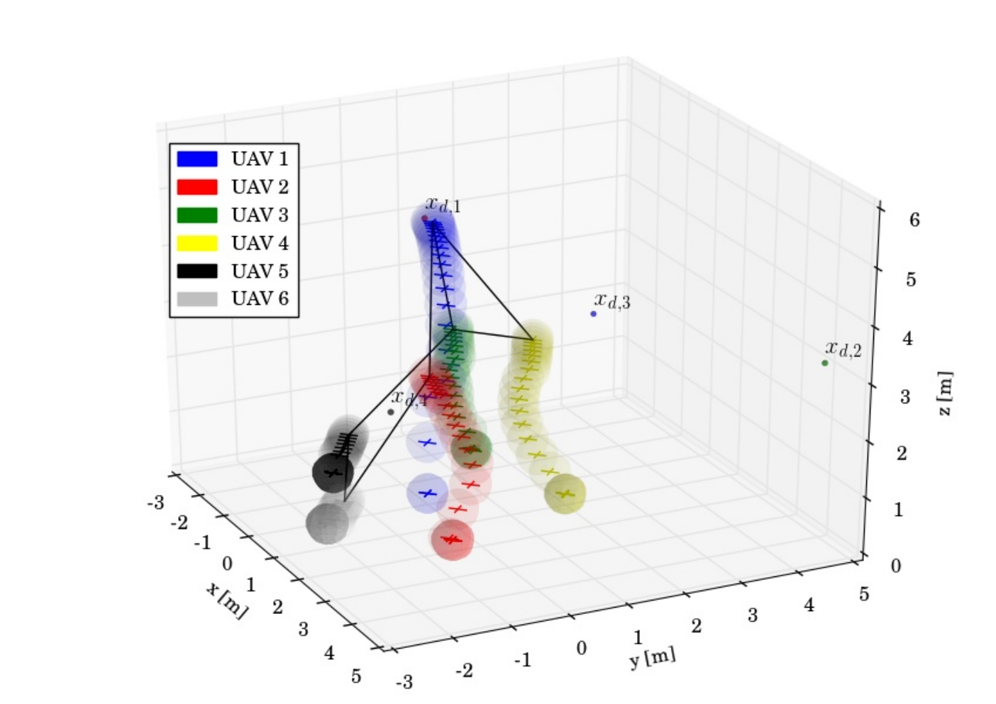
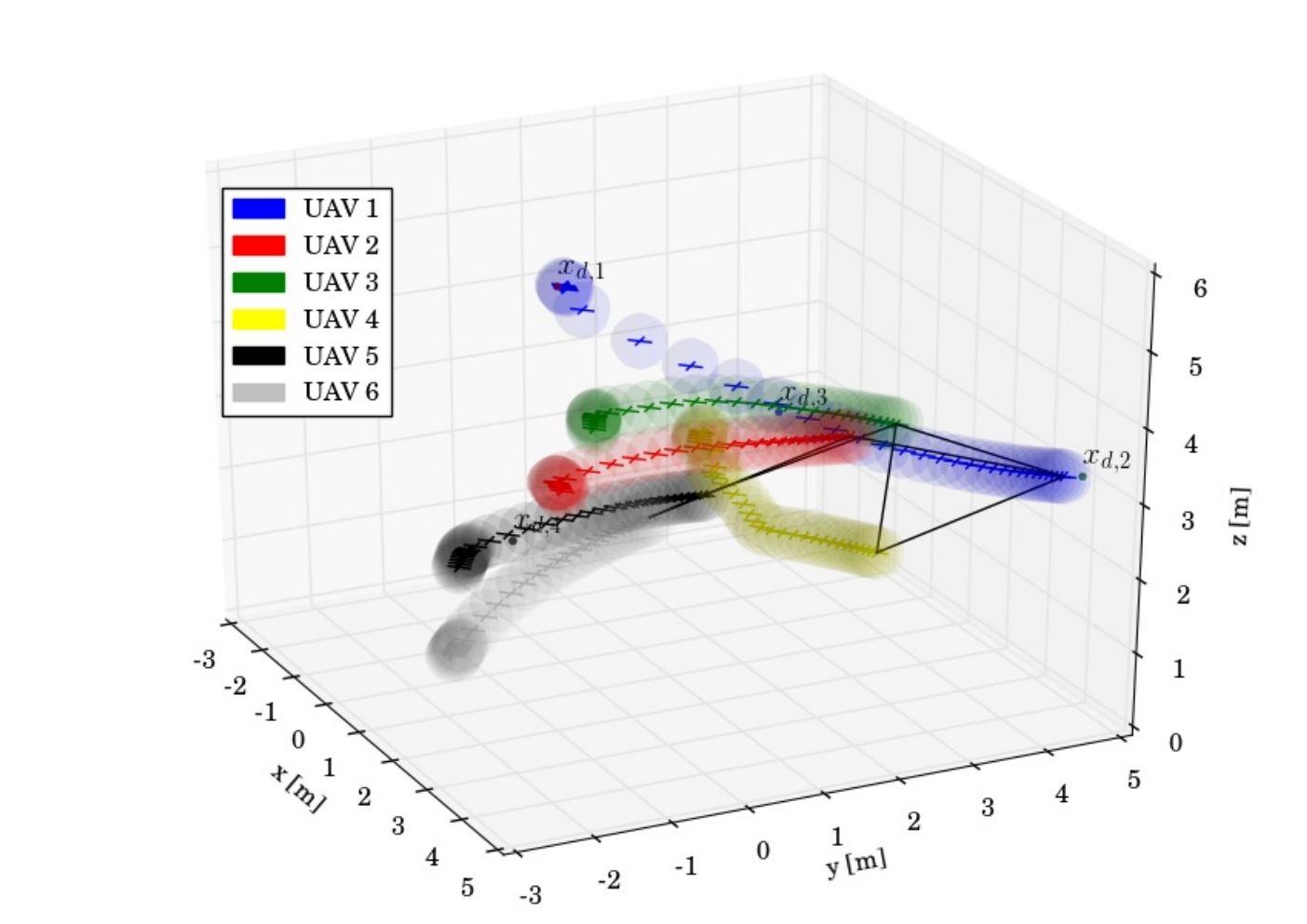
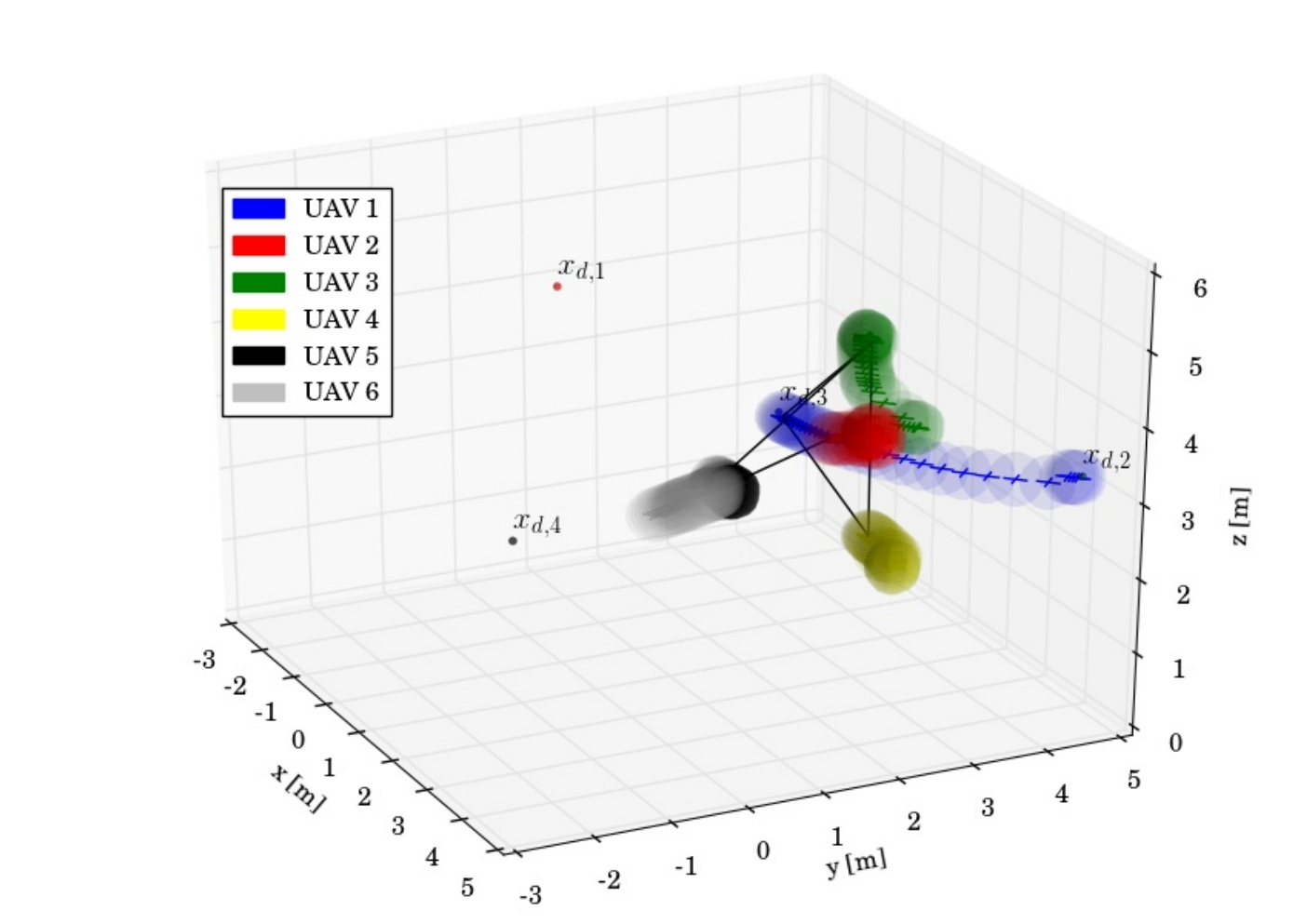
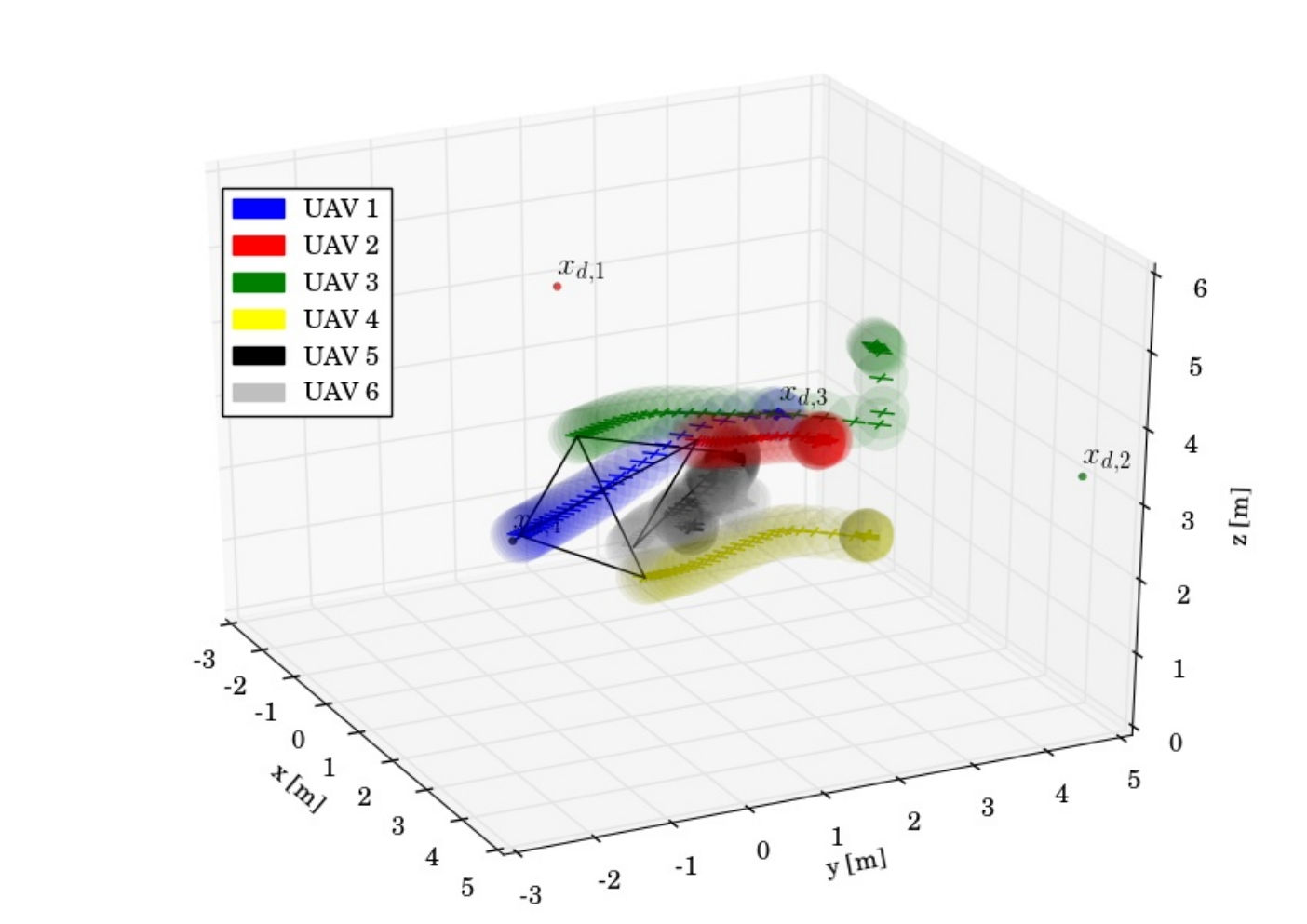
13 Closed-Form Collision Avoidance of Ellipsoidal Multi-Agent Systems
The previous sections, as well as Section 7 of the previous chapter, considered spherical agents, which is a common assumption also in the related literature. In this section, we turn our attention to robotic agents whose volume is approximated as an ellipsoid in , since such an approximation is more realistic for robotic agents (see e.g., Fig. 68). We develop a class of closed-form barrier functions that approximate the distance between two such ellipsoids and design an adaptive control scheme for the collision avoidance of the multi-agent system, subject to some primary task and nd-order uncertain dynamics, like in the previous section.

13.1 Problem Formulation
Consider ellipsoidal autonomous agents, with , operating in , and described now by the ellipsoids
is the th agent’s center of mass pose, where is its inertial position and its unit quaternion-based orientation,with , its scalar and vector parts, respectively, subject to ; , with , corresponding to the principal axis lengths of agent ’s ellipsoid, and is the transformation matrix describing the translation and orientation of agent ’s center of mass, . The agents’ motion follows the standard Lagrangian dynamics (similar to (199)):
| (207a) | ||||
| (207b) | ||||
where is agent ’s velocity, with being its angular velocity, is the matrix mapping the quaternion rates to velocities, defined as and as defined in Section 3.1; The rest of the terms are the same as in (199), with unknown dynamic parameters in , , , and unknown , , . Here we also consider that is decomposed as , where is a bounded term that is responsible for some (potentially cooperative) task, and is a control term to be designed in order to achieve multi-agent decentralized collision avoidance, . More specifically, we consider that is a term that corresponds to the cooperative task dictated by , with
, , for continuous positive definite functions , and nonempty sets , , where , and
can be also a function of that concerns potential formation control objectives. Then becomes
The conditions for are satisfied by standard quadratic functions, e.g.,
(for multi-agent navigation) or
(for formation) for sufficiently distant , where is a potential formation set and represent appropriate quaternion errors (see Section 3.3). Note that and are not responsible for collision avoidance or compensating model uncertainties.
The terms and satisfy Property 4.1, , as well as a slightly modified version of Property 4.2 that accounts only for :
Property 4.3.
The gravity terms of (207) can be written as , , where are known continuous matrices, and , , are constant but unknown dynamic parameters of the agents, .
Moreover, the unknown disturbances satisfy Assumption 4.5 for unknown , , whereas we impose a stronger assumption on for simplicity:
Property 4.4.
[255] The friction terms are dissipative, i.e., , .
As before, we consider that each robot has a limited sensing radius , with the restriction now for an arbitrarily small positive constant , which implies that the agents can sense each other without colliding. Based on this, the undirected time-varying graph that models the topology of the multi-robot network becomes now , with , , and we further define the agent time-varying neighborhood , . Moreover, we consider again the complete graph , with , and an edge numbering set . Finally, we use the same notation for that give the robot indices that form edge .
As discussed before, the agents need to avoid collisions with each other, while executing their task, dictated by . To that end, we aim to design closed-form barrier functions and decentralized feedback control laws that guarantee collision avoidance among the ellipsoidal agents, while compensating appropriately for the model uncertainties and the external disturbances. Formally, the treated problem is the following:
Problem 4.3.
Given D ellipsoidal autonomous agents with the uncertain Lagrangian dynamics (207) executing tasks dictated by , design
- 1.
closed-form barrier functions that encode collision avoidance of the agents,
- 2.
decentralized control laws in that guarantee inter-agent collision avoidance, i.e., , , , as well as boundedness of all closed loop signals.
13.2 Problem Solution
This section describes the proposed solution to Problem 4.3. In order to deal with the ellipsoidal collision avoidance, we employ results from computer graphics that are related to detection of ellipsoid collision and we build appropriate barrier functions whose boundedness implies the collision-free trajectories. Moreover, we use adaptive and discontinuous control laws to appropriately compensate for the uncertainties and external disturbances of (207).
We employ first the results described in Proposition 14.8 of Appendix 14 to build an appropriate ellipsoidal barrier function. Note, however, that these results concern planar ellipsoids and cannot be straightforwardly extended to the D case, which is the case of the considered multi-agent system. For that reason, we consider the respective planar projections. For an ellipsoid , we denote as its projections on the planes -, - and -, respectively, with corresponding matrix terms , i.e.,
Note that in order for to collide (touch externally), all their projections on the three planes must also collide, i.e.,
Therefore, and do not collide if and only if for some . In view of Proposition 14.8 of Appendix 14, that means that the characteristic equations
must always have one positive real root and two negative distinct roots for at least one . Hence, by denoting the discriminant of as , Proposition 14.7 of Appendix 14 suggests that must remain always positive for at least one , since a collision would imply , . Therefore, by defining the smooth function [209]
| (208) |
we conclude that and do not collide if and only if
since a collision would result in . We aim now at defining a decentralized continuously differentiable function for each edge that incorporates the collision avoidance property of agents . We need first the following result regarding the discriminant of :
Proposition 4.2.
Let , be the discriminants of , , respectively, where . Then .
Proof.
Let
with , . It can be verified that
Let be the solutions of , i.e. , and . By substituting in , , we obtain
Hence, are the solutions of . The discriminants of and are
and
respectively, which, by substituting , becomes . ∎
Therefore, we conclude that the discriminants and of and , respectively, are the same, for all . Hence, we can define uniquely for each edge the continuously differentiable function , with
| (209) |
which needs to remain positive for all times in order to achieve the collision avoidance property, i.e., , . Note that, in view of Proposition 4.2, the agents and can calculate (13.2) based on and , respectively, .
We still need to incorporate the fact the that agents have a limited sensing radius, and that agent does not have access to the functions , when . To that end, we define first the greatest lower bound of when both agents are in each other’s sensing radius, i.e.,
| (210) |
Since , , it follows that there exists a positive constant such that . Next, we define the smooth switching functions , with [209]
| (211) |
where is a positive constant satisfying , . Then, by choosing , where is a positive scaling constant, we incorporate the limited sensing radius of the agents in the collision avoidance scheme, since vanishes when or , i.e., when at least one of the agents that form edge lies outside the sensing range of the other agent. Note that are similar to the switches defined in Section 12.2. The terms can be any positive constants, . All the necessary information for the construction of the functions , , i.e., the constants , and the lengths , , , , can be transmitted off-line to the agents.
We can now define a suitable barrier function for each edge as any continuously differentiable function with the property , e.g., , . The barrier function for edge is then , .
We propose now a decentralized feedback control law for the solution of Problem 4.3. Firstly, as in Section 12.2, we define the estimations of the unknown terms and as and , with the respective errors and , . By using adaptive and discontinuous control techniques, we prove in the following that these estimations compensate appropriately for the unknown terms, without necessarily converging to them. In particular, we design the feedback control laws for as
| (212) |
where , , with as defined in Section 13.1. Moreover, if agent is part of edge , and otherwise, , , , , and are positive constant gains. Finally, we design the associated adaptation laws
| (213) |
with arbitrary bounded initial conditions, where and are positive gains, . The correctness of (212)-(213) is shown in the following theorem:
Theorem 4.5.
Consider a multi-agent system comprised of D ellipsoidal agents and subject to the dynamics (207) at a collision-free initial configuration, i.e., , with . Then, application of the control and adaptation laws (212), (213) guarantees that the agents avoid collisions for all times, i.e., , with , , with all closed loop signals being bounded. Moreover, .
Proof.
Consider the vector , , , . Since the initial configuration is collision-free, it holds that . By combining (207), (212), and (213), it can be verified that the conditions of Prop. 3 of Prop. 8.1 in Appendix 8 are satisfied and hence we conclude that at least one Filippov solution exists and any such solution satisfies for a positive . Define
where is the cooperative term defined in Section 13.1. Note that and, for any finite , , which we prove in the following. Define the function
for which it holds that for positive definite functions on . Since , we conclude that is well defined, and hence there exists a finite constant such and , . By differentiating along the solutions of the closed loop system and in view of Lemma 8.2 we obtain . Since is continuously differentiable, the generalized gradient reduces to the standard gradient and therefore, after using Properties 4.1, 4.3, and grouping terms, we obtain
By also using Property 4.4 and Assumption 4.5, substituting with and (212), the adaptation laws (213), and using , and the property , , we obtain
Therefore, , , , where is a positive semi-definite function defined on . Hence, by applying Theorem 8.6 of Appendix 8, we conclude that , is bounded in the compact set , for any and satisfying , , and . Note that, since the sets are nonempty, can be chosen arbitrarily large, corresponding to all collision-free initial configurations. Therefore, inter-agent collisions are avoided, and the adaptation signals , , remain bounded, , . The continuity of the terms implies also their boundedness and hence the boundedness of the control signals (212), (213), . ∎
Remark 4.6.
It can be verified that , and hence , are functions of , , . Therefore, if is a function of , the aforementioned analysis still holds by setting . Moreover, note that achievement of the objectives expressed by is not pursued here and may not be necessarily guaranteed due to the potentially counteracting terms of .
Remark 4.7.
Since (due to Proposition 4.2), , , the control scheme can be extended to directed communication graphs, by setting for the th agent , , with as in (13.2) and as in (211), as in (210), and appropriately modifying the control law. Similarly, collision avoidance with static environment obstacles could be incorporated in the overall scheme.
13.3 Simulation Results
We consider a simulation example with rigid bodies in , described by ellipsoids with axes lengths m, m, m, . The initial poses are (in m)
| , | |
| , | |
| , | |
| , |
We consider that describes an independent multi-agent navigation objective, with desired configurations as
and ,,,, . We set the errors and , and are the scalar and vector parts, respectively, of the quaternion error (see Section 3 ). The desired quaternion configuration is achieved when and hence the function is chosen as
with
The control inputs are therefore chosen as
. The agent masses and moments of inertia are chosen randomly in the interval . We also set , , , with the terms , , and chosen randomly in the interval , . We choose , with , , , , and , , , . The expressions for were derived by using the symbolic toolbox of MATLAB. Fig. 69 shows a D plot of the agent trajectories, and Fig. 70 shows the minimum of the barrier functions (left), which is always positive, and the signals and (right), , . Finally, Fig. 71 depicts the control inputs of the agents. A short video that demonstrates the aforementioned simulation example can be found in https://youtu.be/IAni7zIMM7k.
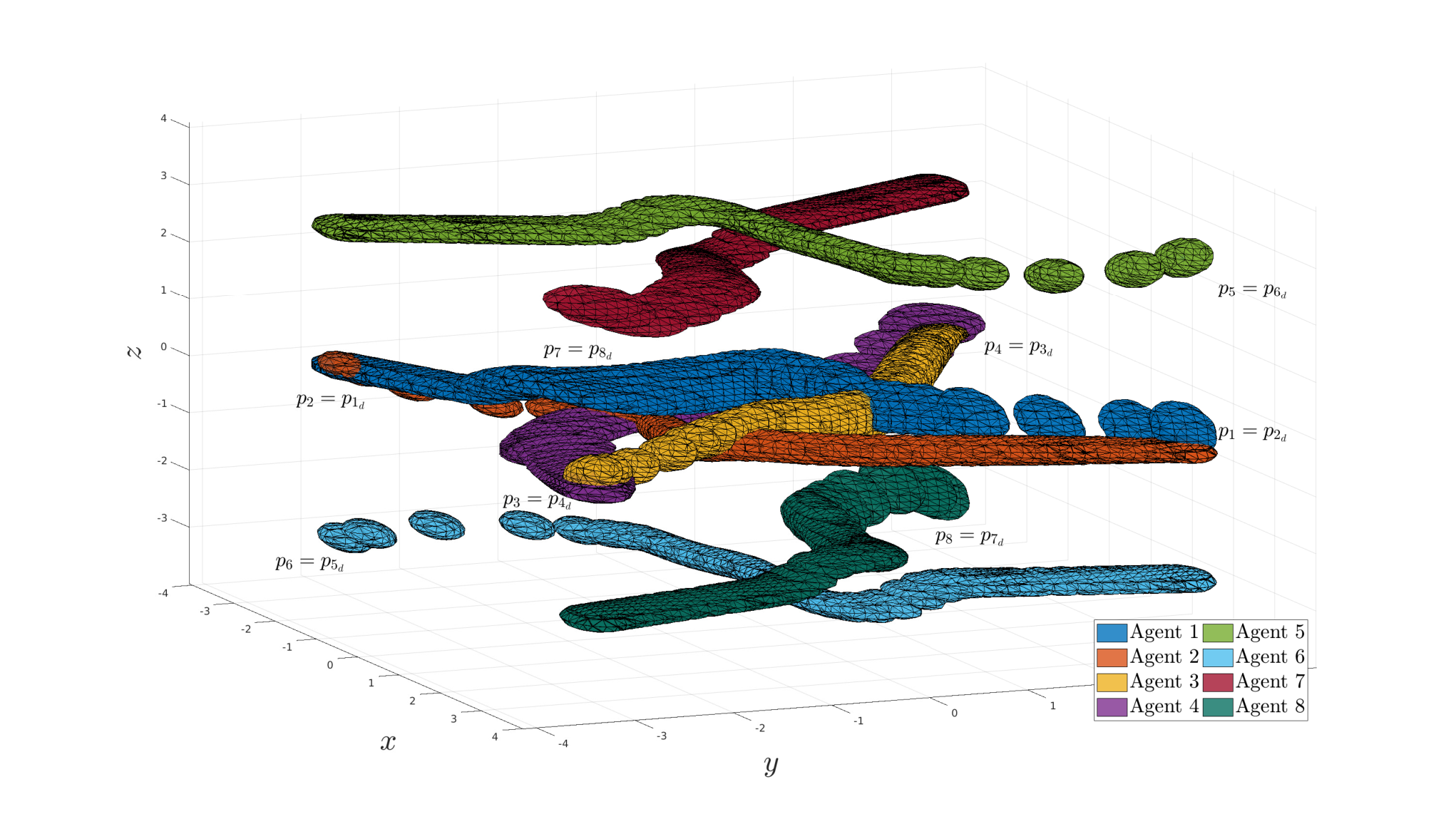

14 Conclusion
This chapter presented several continuous control algorithms for multi-agent coordination of systems with uncertain dynamics. Firstly, we develop an adaptive control scheme for the almost global navigation of a single robotic agent in a workspace with obstacles, which is then extended to a decentralized multi-robot scheme. Secondly, we develop a decentralized adaptive multi-agent algorithm for the leader-follower coordination: A leader agent converges to a predefined goal point while the entire team avoids collision with each other and maintains connectivity. Finally, we develop a closed-form barrier function that encodes the distance between D ellipsoids, and design a decentralized collision avoidance control scheme for a team of ellipsoidal robotic agents, while compensating for the dynamic uncertainties.
Chapter 5 Abstractions of Multi-Agent and Multi-Agent-Object Systems
After designing continuous solutions to multi-agent problems, such as cooperative manipulation, formation, and navigation, we are ready to transit to the problem of multi-agent planning under temporal logic tasks. The content of the previous chapters can act as a means to obtain well-defined discrete representations (abstractions) of the continuous systems in hand. Therefore, this chapter addresses the motion and task planning of multi-agent and multi-agent-object systems (systems comprised of multiple robotic agents and objects) subject to temporal logic constraints, focusing both on the abstraction technique as well as the control synthesis for the accomplishment of the tasks.
More specifically, this chapter can be divided in two main parts. The first part tackles the motion planning of multi-robot teams under local linear temporal tasks, i.e., when each robotic agent has its own task. The second part addresses the case where unactuated objects of the workspace must satisfy a certain temporal logic task, with the robotic agents being responsible for their accomplishment.
15 Introduction
Temporal-logic-based motion planning has gained significant attention in recent years, as it provides a fully automated correct-by-design controller synthesis approach for autonomous robots. Temporal logics such as linear temporal logic (LTL) and metric interval temporal logic (MITL) provide formal high-level languages that can describe complex planning objectives. As already discussed in the previous chapters, standard control problems are restricted to point-to-point navigation, multi-agent formation control, or consensus. Ultimately, however, we would like the robotic agents to execute more complex high-level tasks, involving combinations of safety (”never enter a dangerous regions”), surveillance (”keep visiting regions and infinitely often”) or sequencing (”collect data in region and upload it in region ”) properties. Temporal logic languages offer a means to express the aforementioned specifications, since they can describe complex planning objectives in a more efficient way than the well-studied navigation algorithms. The task specification is given as a temporal logic formula with respect to the discretized abstraction of the robot motion modeled as a finite transition system [256, 257, 258, 259]. Then a high-level discrete plan is found by off-the-shelf model-checking algorithms, given the finite transition system and the task specification [260]. Temporal logics have been extensively used in the related literature for both single- and multi-agent systems, e.g., [261, 262, 263, 264, 265, 266, 267, 268, 269, 270, 271, 272, 257, 258, 273, 274, 275].
A special and important class of autonomous robotic systems is the class of unmanned aerial vehicles (UAV), which can provide efficient multi-agent solutions in several problems, e.g., coverage or inspection. Control of aerial vehicles in a multi-agent setting has been well studied in the related literature. The standard problem of formation control for a team of aerial vehicles is addressed in [276, 277, 278, 279, 280, 281], whereas [282, 283, 284, 285, 286] consider leader-follower formation approaches, where the latter also treats the problem of collision avoidance with static obstacles in the environment; [287], [288, 289] and [290] employ dynamic programming, Model Predictive Control and reachable set algorithms, respectively, for inter-agent collision avoidance, which is tackled also in [291]. In [292] the cooperative evader pursuit problem is treated. Aerial vehicles and temporal logic-based planning is considered in [293], which addresses the vehicle routing problem using MTL specifications and in [294], which approaches the LTL motion planning using MILP optimization techniques, both in a centralized manner. Markov Decision Processes are used for the LTL planning in [295]. The aforementioned works, however, consider discrete agent models and do not take into account their continuous dynamics.
The discretization of a multi-agent system to an abstracted finite transition system necessitates the design of appropriate continuous-time controllers for the transition of the agents among the states of the transition system [260]. Most works in the related literature, however, including the aforementioned ones, either assume that there exist such continuous controllers or adopt single- and double-integrator models, ignoring the actual dynamics of the agents. Discretized abstractions, including design of the discrete state space and/or continuous-time controllers, have been considered in [296, 297, 298, 299, 300] for general systems and [301, 302] for multi-agent systems.
Another drawback of the majority of works in the related literature of temporal logic-based motion planning is the point-agent assumption (as, e.g. in [264, 269, 268]), which does not take into account potential collisions between the robotic agents. The latter is a crucial safety property in real-time scenarios, where actual vehicles are used in the motion planning framework.
Furthermore, most works in the related literature consider temporal logic-based motion planning for fully actuated, autonomous agents. Consider, however, cases where some unactuated objects must undergo a series of processes in a workspace with autonomous agents (e.g., car factories). In such cases, the agents, except for satisfying their own motion specifications, are also responsible for coordinating with each other in order to transport the objects around the workspace. When the unactuated objects’ specifications are expressed using temporal logics, then the abstraction of the agents’ behavior becomes much more complex, since it has to take into account the objects’ goals. More specifically, we are here interested in complex tasks, possibly including time, such as “never take the object to dangerous regions” or “keep moving the object from region A to B within a predefined time interval” which must be executed via the control actions of the robotic agents. Time constraints can be incorporated in the motion planning temporal logic-based problem via specific logics, such as Metric and Metric Interval Temporal Logic (MTL, MITL) [303, 304, 305], as well as Time Window Temporal Logic (TWTL), or Signal Temporal Logic (STL). Such languages have been for multi-agent motion planning in several works (e.g., [306, 307, 272, 308]).
This chapter addresses the motion planning problem of multi-agent systems as well multi-agent-object systems subject to complex tasks, expressed as temporal logic specifications. Firstly, we develop decentralized control protocols for the navigation of a multi-robot team among predefined regions or interest in the workspace, while taking into collision and/or connectivity properties. We consider separately the cases of (i) aerial vehicles, and (ii) mobile robotic manipulators. This allows us to abstract the continuous multi-agent dynamics as discrete transition systems (abstractions), which then can be used to obtain a path that satisfies the given local LTL specifications, by employing formal method-based methodologies.
Secondly, we provide, similar to the first case, appropriate discrete abstractions for multi-robot-object systems, encoding the behavior of the robots as well as the unactuated objects in the workspace. The proposed abstraction design involves both multi-robot safe navigation as well as cooperative object transportation. The abstracted systems are then used to derive paths that satisfy the robotic agents’ and the objects’ (possibly timed) temporal goals.
Although the proposed control schemes from the previous chapters can be used, we provide new control ideas as alternatives for the derivation of the discrete abstractions.
16 Decentralized Motion Planning with Collision Avoidance for a Team of UAVs under High Level Goals
We first describe a decentralized hybrid control algorithm for the motion planning of aerial vehicles subject to Linear Temporal Logic (LTL) specifications.
16.1 Problem Formulation
Consider aerial agents operating in a static workspace that is bounded by a large sphere in -D space , where and are the center and radius of . Within there exist smaller spheres around points of interest, which are described by , where are the central point and radius, respectively, of . We denote the set of all as . Moreover, we introduce a set of atomic propositions for each agent that indicates certain properties of interest of agent in and are expressed as boolean variables. The properties satisfied at each region are provided by the labeling function , which assigns to each region the subset of the atomic propositions that are true in that region.

Each agent occupies a bounding sphere , where is the center and the radius of the sphere (Fig. 72). We also consider that , i.e., the regions of interest are larger than the aerial vehicles. The motion of each agent is controlled via its centroid through the single integrator dynamics:
| (214) |
Moreover, similar to the previous chapter, we consider that agent has a limited sensing range of . Therefore, by defining the neighboring set , agent knows at each configuration the position of all as well as its own position . The workspace is assumed to be perfectly known, i.e., are known to all agents, for all .
With the above ingredients, we provide the following definitions:
Definition 5.1.
An agent is in a region at a configuration , denoted as , if and only if .
Definition 5.2.
Assume that for some . Then there exists a transition for agent from region to region , denoted as , if and only if there exists a finite such that
- 1.
,
- 2.
,
- 3.
,
- 4.
with with and .
Loosely speaking, an agent can transit between two regions of interest and , if there exists a bounded control trajectory in (214) that takes agent from to while avoiding entering all other regions, colliding with the other agents, or exiting the workspace boundary.
Our goal is to control the multi-agent system subject to (214) so that each agent’s behavior obeys a given specification over its atomic propositions .
Definition 5.3.
Given a trajectory of agent , its corresponding behavior is given by the infinite sequence , with and .
The satisfaction of a LTL formula is provided by the following definition (see Appendix 13 for more details on LTL formulas).
Definition 5.4.
The behavior satisfies an LTL formula if and only if .
The control objectives are given for each agent separately as LTL formulas over . An LTL formula is satisfied if there exists a behavior of agent that satisfies . Formally, the problem treated in this section is the following:
Problem 5.1.
Given a set of aerial vehicles subject to the dynamics (214) and LTL formulas over the respective atomic propositions , achieve behaviors that (i) yield satisfaction of and (ii) guarantee inter-agent collision avoidance.
16.2 Problem Solution
We provide here the proposed solution to Problem 5.1, which consists of two main layers, that is, the design of a continuous control scheme, and the derivation of a high level path that satisfies .
16.2.1 Continuous Control Design
The first ingredient of our solution is the development of a decentralized feedback control law that establishes a transition relation according to Def. 5.2. The proposed approach is based on the concept of Decentralized Navigation Functions, introduced in [309], for which an overview can be found in Appendix 10. More specifically, given that for some , we propose a decentralized control law for the transition , as defined in Def. 5.2.
Initially, we define the set of “undesired” regions as and the corresponding free space , with . As the goal configuration we consider the centroid of and we construct the function with . For the collision avoidance between the agents, we employ the function as defined in [309], which encodes the distances among the agents.
Moreover, we need some extra terms that guarantee that agent will avoid the rest of the regions as well as the workspace boundary. To this end, we construct the function with , where the function is a measure of the distance of agent from the workspace boundary and the function is a measure of the distance of agent from the undesired regions .
With the above ingredients, we construct the following navigation function :
for agent , with and the following vector field:
| (215) |
for all , with and , defined in [309], is a term that handles inter-agent collisions when an agent has reached its destination.
The navigation field (215) guarantees that agent will not enter the undesired regions or collide with the other agents and . The latter property of asymptotic convergence along with the assumption that , implies that there exists a finite time instant such that and more specifically that , which is the desired behavior. The time instant can be chosen from the set .
Note, however, that once agent leaves region , there is no guarantee that it will not enter that region again (note that includes ), which might be undesirable. Therefore, we define the set and the corresponding free space , and we construct the function :
where , with corresponding vector field:
| (216) |
which guarantees that region will be also avoided. Therefore, we develop a switching control protocol that employs (215) until agent is out of region and then switches to (216) until . Consider the following switching function:
and the time instant that represents the moment that agent is out of region , i.e., . Then, we propose the following switching control protocol :
| (217) |
where , and is a design parameter indicating the time period of the switching process, with . Invoking the continuity of , we obtain and hence the control protocol (217) guarantees, for sufficiently small , that agent will navigate from to in finite time without entering any other regions or colliding with other agents and therefore establishes a transition .
16.2.2 High-Level Plan Generation
The next step of our solution is the high-level plan, which can be generated using standard techniques inspired by automata-based formal verification methodologies. In Section 16.2.1, we proposed a continuous control law that allows the agents to transit between any in the given workspace , without colliding with each other. Thanks to this and to our definition of LTL semantics over the sequence of atomic propositions, we can abstract the motion capabilities of each agent as a finite transition system as follows [260]:
Definition 5.5.
The motion of each agent in is modeled by the following Transition System (TS):
where is the set of states represented by the regions of interest that the agent can be at, according to Def. 5.1, is the set of initial states that agent can start from, is the transition relation established in Section 16.2.1, and are the atomic propositions and labeling function respectively, as defined in Section 16.1.
After the definition of , we translate each given LTL formula into a Büchi automaton and we form the product . The accepting runs of satisfy and are directly projected to a sequence of waypoints to be visited, providing therefore a desired path for agent . Although the semantics of LTL is defined over infinite sequences of atomic propositions, it can be proven that there always exists a high-level plan that takes a form of a finite state sequence followed by an infinite repetition of another finite state sequence. For more details on the followed technique, we kindly refer the reader to the related literature, e.g., [260].
Following the aforementioned methodology, we obtain a high-level plan for each agent as sequences of regions and atomic propositions and with and .
The execution of produces a trajectory that corresponds to the behavior , with and , . Therefore, since , the behavior yields satisfaction of the formula . Moreover, the property of inter-agent collision avoidance is inherent in the transition relations of and guaranteed by the navigation control algorithm of Section 16.2.1.
Remark 5.1.
The proposed control algorithm is decentralized in the sense that each agent derives and executes its own plan without communicating with the rest of the team. The only information that each agent has is the position of its neighboring agents that lie in its limited sensing radius. It is worth mentioning, nevertheless, that the workspace boundary and regions of interest have to satisfy certain assumptions, such as having a sufficient distance from each other or being sufficiently sparse.


16.3 Simulation and Experimental Results
To demonstrate the efficiency of the proposed algorithm, we consider aerial vehicles with m, m, , operating in a workspace with m and m. Moreover, we consider spherical regions of interest with m, and m, m, m, m and m. The initial configurations of the agents are taken as and therefore, and . An illustration of the described workspace is depicted in Fig. 73.


We consider that agent is assigned with inspection tasks and has the atomic propositions with , and , where we have considered that region is an undesired (“obstacle”) region for this agent. More specifically, the task for agent is the continuous inspection of the workspace while avoiding region . The corresponding LTL specification is . Agents and are interested in moving around resources scattered in the workspace and have propositions with and . We assume that is shared between the two agents whereas and have to be accessed only by agent and and only by agent . The corresponding specifications are and , where we have also included a specific order for the access of the resources. Next, we employ the off-the-shelf tool LTL2BA [310] to create the Büchi automata and by following the procedure described in Section 16.2.2, we derive the paths , whose execution satisfies . Regarding the continuous control protocol, we chose in (215), (216) and the switching duration in (217) was calculated online as , where we assume that the large distance between the regions (see Fig. 73) implies that and thus, . The simulation results are depicted in Fig. 74 and 76. In particular, Fig. 76 illustrates the execution of the paths and by agents and respectively, where the superscript here denotes that the corresponding paths are executed twice. Fig. 74 depicts the resulting control inputs . The figures demonstrate the successful execution of the agents’ paths and therefore, satisfaction of the respective formulas with inter-agent collision avoidance.


The validity and efficiency of the proposed solution was also verified through real-time experiments. The experimental setup involved two remotely controlled IRIS+ quadrotors from D Robotics, which we consider to have sensing range m, upper control input bound m/s, , and bounding spheres with radius m, . We considered two -dimensional scenarios in a workspace with and m.
The first scenario included regions of interest in , with and m, m, m and m. The initial positions of the agents were taken such that and (see Fig. 75). We also defined the atomic propositions with . In this scenario, we were interested in area inspection while avoiding the “obstacle” region, and thus, we defined the individual specifications with the following LTL formulas: . By following the procedure described in Section 16.2.2, we obtained the paths . Fig. 77 depicts the execution of the paths and by agents and , respectively, and Fig. 78 shows the corresponding input signals, which do not exceed the control bounds m/s. It can be deduced by the figures that the agents successfully satisfy their individual formulas, without colliding with each other.
The second experimental scenario included regions of interest in , with and m, m and m. The initial positions of the agents were taken such that and (see Fig. 79). We also defined the atomic propositions , corresponding to a base and several resources in the workspace, with . We considered that the agents had to transfer the resources to the “base” in ; both agents were responsible for but only agent should access . The specifications were translated to the formulas and the derived paths were and . The execution of the paths and by agents 1 and 2, respectively, are depicted in Fig. 81, and the corresponding control inputs are shown in Fig. 80. The figures demonstrate the successful execution and satisfaction of the paths and formulas, respectively, and the compliance with the control input bounds.
Regarding the continuous control protocol in the aforementioned experiments, we chose in (215), (216) and the switching duration in (217) as .


The simulations and experiments were conducted in Python environment using an Intel Core i7 2.4 GHz personal computer with 4 GB of RAM, and are clearly demonstrated in the video found in https://youtu.be/dO77ZYEFHlE.
17 Robust Decentralized Abstractions for Multiple Mobile Manipulators
We now turn our attention to a class of more complex systems, that is, mobile manipulators, which, unlike the previous section, have more complex and uncertain dynamics. In fact, we provide a more explicit dynamics formulation than just a sphere/ellipsoid, which was done so far. We describe a decentralized control algorithm that allows the derivation of a discrete abstraction of the multi-agent dynamics.
17.1 Problem Formulation

Like before, consider fully actuated agents, with index set , composed by a robotic arm mounted on an omnidirectional mobile base, operating in a static workspace that is bounded by a large sphere in D space, i.e. , where is the center of , and is its radius. Without loss of generality, we consider that , corresponding to an inertial frame of reference. As in the previous section, we consider that within there exist disjoint spheres around points of interest, which are described by , where and are the center and radius of the th region, respectively. The regions of interest can be equivalently described by , where is the vector of homogeneous coordinates of , and
The dynamic model of each agent is given by the second-order Lagrangian dynamics (see (1) of Chapter 2):
| (218) |
, where is the vector of generalized coordinates (e.g., pose of mobile base and joint coordinates of the arms), with , and the rest of the terms as in (1) with a slight change of notation; here represents friction-like terms. Without loss of generality, we assume that . In addition, we denote by the inertial position of the mobile base of agent . Moreover, the matrix is skew-symmetric [311], and we further make the following assumption, similar to Assumption 4.1:
Assumption 5.1.
There exist positive constants such that , , .
For the inter-agent collisions, we will use the ideas of Section 13 and ellipsoid collision. We consider hence that each agent is composed by rigid links (see Fig. 82) with the corresponding index set. Each link of agent is approximated by the ellipsoid set [312] ; is the homogeneous coordinates of , and is defined as , where corresponds to the positive lengths of the principal axes of the ellipsoid, and is the transformation matrix for the coordinate frame placed at the center of mass of the -th link of agent , aligned with the principal axes of :
with being the rotation matrix of the link, . For an ellipsoid , we denote by its projections on the planes -, - and -, respectively, with corresponding matrix terms .
By following the procedure of Section 13, we conclude that a sufficient condition for and not to collide is , with as defined in (208) and is the discriminant of the equation , , , , , where the subscript stands for the planar ellipsoid matrices.
Next, we define the constant , which is the maximum distance of the base to a point in the agent’s volume over all possible configurations, i.e. . We also denote . Moreover, we consider that each agent has a sensor located at the center of its mobile base with a sensing radius , where is an arbitrarily small positive constant. Hence, each agent has the sensing sphere and its neighborhood set at each time instant is defined as .
As in Section 16.1, we are interested in defining transition systems for the motion of the agents in the workspace in order to be able to assign complex high level goals through logic formulas. Moreover, since many applications necessitate the cooperation of the agents in order to execute some task (e.g. transport an object), we consider that a nonempty subset , of the initial neighbors of the agents must stay connected through their motion in the workspace, similarly to Section 12. In addition, it follows that the transition system of each agent must contain information regarding the current position of its neighbors. The problem in hand is equivalent to designing decentralized control laws , for the appropriate transitions of the agents among the predefined regions of interest in the workspace.
Definition 5.6.
An agent is in region at a configuration , denoted as , if and only if , .
Definition 5.7.
Agents , with , are in collision-free configurations , denoted as , if and only if .
Given the aforementioned discussion, we make the following assumptions regarding the agents and the validity of the workspace
Assumption 5.2.
The regions of interest are
- (i)
large enough such that all the agents can fit, i.e., given a specific , there exist , such that , , with , , with .
- (ii)
sufficiently far from each other and the obstacle workspace, i.e.,
, where is an arbitrarily small positive constant.
Next, in order to proceed, we need the following definition.
Definition 5.8.
Assume that , for some , with . There exists a transition for agent between and , denoted as , if and only if there exists a finite time , such that
- •
- •
, ,
- •
, ,
- •
, ,
- •
, ,
.
Given the aforementioned definitions, the treated problem is the design of decentralized control laws for the transitions of the agents between two regions of interest in the workspace, while preventing collisions of the agents with each other, the workspace boundary, and the remaining regions of interest. More specifically, we aim to design a finite transition system for each agent of the form [260]
| (219) |
where is the set of regions of interest that the agents can be at, according to Def. 5.6, is a set of initial regions that each agent can start from, is the transition relation of Def. 5.8, is a set of given atomic propositions, represented as boolean variables, that hold in the regions of interest, is a labeling function, and is a function that maps the region that agent occupies to the regions the initial neighbors of agent are at. Therefore, the treated problem is the design of bounded controllers for the establishment of the transitions . Moreover, as discussed before, the control protocol should also guarantee the connectivity maintenance of a subset of the initial neighbors . Another desired property important in applications involving robotic manipulators, is the nonsingularity of the Jacobian matrix , that transforms the generalized coordinate rates of agent to generalized velocities [311] (also defined in Chapter 2). That is, the agents should always remain in the sets , .
Formally, we define the problem treated in this section as follows:
Problem 5.2.
Consider mobile manipulators with dynamics (218) and regions of interest , with , , and .
Given nonempty subsets of the initial edge sets , as well as the indices , such that , design decentralized controllers such that, for all :
- 1.
, for some ,
- 2.
,
- 3.
,
- 4.
.
The aforementioned specifications concern 1) the agent transitions according to Def. 5.8, 2) the confinement of the agents in , 3) the connectivity maintenance between a subset of initially connected agents and 4) the agent singularity avoidance. Moreover, the fact that the initial edge sets are nonempty implies that the sensing radius of each agent covers the regions of the agents in the neighboring set . Similarly, the condition , is a feasibility condition for the goal regions, since otherwise it would be impossible for two initially connected agents to stay connected. Intuitively, the sensing radii should be large enough to allow transitions of the multi-agent system to the entire workspace.
17.2 Problem Solution
To solve Problem 5.2, we use the concept of potential fields, as done in Section 16. Nevertheless, we do not provide an explicit closed-form expression of the potential function, but provide appropriate conditions.
Let be a decentralized potential function, with the following properties:
- (i)
The function is not defined, i.e., , , when a collision or a connectivity break occurs,
- (ii)
The critical points of where the vector field vanishes, i.e., the points where , consist of the goal configurations and a set of configurations whose region of attraction (by following the negated vector field curves) is a set of measure zero.
- (iii)
It holds that and
, .
More specifically, is a function of two main terms, a goal function , which should vanish when , and an obstacle function, that encodes inter-agent collisions, collisions between the agents and the obstacle boundary/undesired regions of interest, connectivity losses between initially connected agents and singularities of the Jacobian matrix ; Next, we provide an analytic construction of the goal and obstacle terms. However, the construction of the function is not taken into account.
The control objective of agent , i.e., reaching the region of interest , is encoded in the function , defined as
where is a configuration such that , for an arbitrarily small positive constant , which implies , . In case that multiple agents have the same target, i.e., there exists at least one such that , then we assume that .
Inter-agent collisions, collisions with the boundary of the workspace and the undesired regions of interest, connectivity between initially connected agents and singularities of the Jacobian matrix are encoded by a function , defined next.
As mentioned before, a sufficient condition for ellipsoids and not to collide, is , , and as defined in (208).
Additionally, we define the greatest lower bound of the when the point is on the boundary of the sensing radius of agent , as . Since , it follows that there exists a positive constant such that .
We further define the function , with , and the distance functions , as
where is a constant satisfying , and are strictly increasing polynomials appropriately selected to guarantee that the functions , and , respectively, are twice continuously differentiable everywhere, with . Note that the functions defined above use only local information in the sensing range of agent . Similarly, encodes the collision of agent with the workspace boundary.
Finally, we choose the function as
, where . Note that we have included the term to also account for singularities of and the term takes into account also the collisions between the ellipsoidal rigid bodies of agent .
With the introduced notation, the properties of the functions are:
- (i)
,
- (ii)
and the regions of attraction of the points , are sets of measure zero.
By further denoting , we are ready to state the main theorem of this section:
Theorem 5.1.
Under the Assumptions 5.1-5.2, the decentralized control laws , with
| (220) |
with positive gain constants, , along with the adaptation laws
| (221) |
with positive gain constants, , guarantee the transitions for finite for almost all initial conditions, while ensuring , as well as the boundedness of all closed loop signals, providing, therefore, a solution to Problem 5.2.
Proof.
The closed loop system of (218) is written as:
| (222) |
. Due to Assumption 5.2, the domain where the functions are well-defined (i.e., where ) is connected. Hence, consider the Lyapunov-like function , with
where and are the stack vectors containing all and , respectively, , and . Note that, since there are no collision or singularities at , the functions , are strictly positive at which implies the boundedness of at . Therefore, since and , there exists a positive and finite constant such that .
By differentiating , substituting the dynamics (218), employing the skew symmetry of as well as , we obtain
which, by substituting the control and adaptation laws (220) and (221), becomes:
where we have used the property . Since , we obtain , which implies that is non-increasing along the trajectories of the closed loop system. Hence, we conclude that , as well as the boundedness of and hence of . Therefore, we conclude that .
Hence, inter-agent collisions, collision with the undesired regions and the obstacle boundary, connectivity losses between the subsets of the initially connected agents and singularity configurations are avoided.
Moreover, by invoking LaSalle’s Invariance Principle, the system converges to the largest invariant set contained in
One can easily conclude that , in and thus we conclude for the closed loop system (222) that , since , in view of Assumption 5.1. Therefore, by invoking the properties of , each agent will converge to a critical point of , i.e., all the configurations where . However, due to properties of , the initial conditions that lead to configurations such that and are sets of measure zero in the configuration space [313]. Hence, the agents will converge to the configurations where from almost all initial conditions, i.e., . Therefore, since , it can be concluded that there exists a finite time instance such that , and hence, each agent will be at its goal region at time . In addition, the boundedness of implies the boundedness of the adaptation laws . Hence, the control laws (220) are also bounded.
∎
17.2.1 Hybrid Control Framework
Due to the proposed continuous control protocol, the transitions of Problem 5.2 are well-defined, according to Def. 5.8. Moreover, since all the agents remain connected with the subset of their initial neighbors and there exist finite constants , such that , all the agents are aware of their neighbors state, when a transition is performed. Hence, the transition system (219) is well defined, . Consider, therefore, that , as well as a given desired path for each agent, that does not violate the connectivity condition of Problem 5.2. Then, the iterative application of the control protocol (220) for each transition of the desired path of agent guarantees the successful execution of the desired paths, with all the closed loop signals being bounded.
Remark 5.2.
Note that, according to the aforementioned analysis, we implicitly assume that the agents start executing their respective transitions at the same time (we do not take into account individual control jumps in the Lyapunov analysis, i.e., it is valid only for one transition). Intuition suggests that if the regions of interest are sufficiently far from each other, then the agents will be able to perform the sequence of their transitions independently. Detailed technical analysis of such cases is part of future research.
17.3 Simulation Results
To demonstrate the validity of the proposed methodology, we consider the simplified example of three agents in a workspace with m and three regions of interest, with m, . Each agent consists of a mobile base and a rigid link connected with a rotational joint, with m, . We also choose m, m, m. The initial base positions are taken as , which imply that and (see Fig. 83(a). The control inputs for the agents are the D force acting on the mobile base, and the joint torque of the link. We also consider a sensing radius of and the subsets of initial neighbors as , and , i.e., agent has to stay connected with agent , agent has to stay connected with agents and and agent has to stay connected with agent . The agents are required to perform two transitions. Regarding the first transition, we choose for agent for agent , and , for agent . Regarding the second transition, we choose , and . The control parameters and gains are chosen as , and . We employ the potential field from [309]. The simulation results are depicted in Fig. 83-86. In particular, Fig. 83(b) and 83(c) illustrate the two consecutive transitions of the agents. Fig. 84 depicts the obstacle functions which are strictly positive, . Finally, the control inputs are given in Fig. 85 and the parameter errors are shown in Fig. 86, which indicates their boundedness. As proven in the theoretical analysis, the transitions are successfully performed while satisfying all the desired specifications.
18 Timed Abstractions for Distributed Cooperative Manipulation
We now switch our attention to multi-agent-object systems. Such systems include, except for a number of robotic agents, a certain number of unactuated objects (items in the environment). We consider that these objects, along with the agents, have themselves some local tasks to complete, expressed as temporal specifications with respect to their locations. This section considers the problem of motion planning for one unactuated object, which is grasped by a number of robotic agents, under timed temporal specifications, and in particular, Metric Interval Temporal Logic (MITL) specifications. In particular, we design appropriate well-defined timed abstractions for a cooperatively manipulated object that allows us to express and solve the object motion planning problem under MITL formulas.
18.1 Problem Formulation
Consider a bounded workspace containing robotic agents rigidly grasping an object, similar to what is shown in Fig. 2. The agents are considered to be fully actuated and they consist of a base that is able to move around the workspace (e.g., mobile or aerial vehicle) and a robotic arm. The setup considered here is the same as in Section 3, which we briefly recap. Each agent knows only its own state, position and velocity, as well as its own and the object’s geometric parameters. More specifically, we assume that each agent knows the distance from its grasping point to the object’s center of mass as well as the relative orientation offset between the two frames and . This information can be either retrieved on-line via appropriate sensors or transmitted off-line to the agents, without the need of inter-agent on-line communication. Finally, no interaction force/torque measurements are required and the dynamic model of the object and the agents is considered unknown.
The dynamics of the agents are (see eq. (3))
whereas the object’s
and the coupled dynamics by
| (223) |
with the coupling terms as in (15) and .


18.1.1 Workspace Partition
As already mentioned, we are interested in designing a well-defined abstraction of the coupled object-agents system, so that we can define MITL formulas over certain properties in a discrete set of regions of the workspace. Therefore, we provide now a partition of into cell regions. We denote by the set that consists of all points that physically belong to the coupled system, i.e., they consist part of either the volume of the agents or the volume of the object. Note that these points depend on the actual value of . We further define the constant , where, with a slight abuse of notation and in view of the coupled object-agents kinematics and the forward kinematics of the agents, we express as a function of . Note that, although the explicit computation of may not be possible, is an upper bound of the maximum distance between the object center of mass and a point in the coupled system’s volume over all possible configurations , and thus, it can be measured. For instance, Fig. 87 shows for the system of Fig. 2. It is straightforward to conclude that
| (224) |
Next, we partition the workspace into equally sized rectangular regions , whose geometric centers are denoted by . The length of the region sides is set to , where is an arbitrary positive constant. Hence, each region can be formally defined as follows:
with , and ; , denotes the -th coordinate. An illustration of the aforementioned partition is depicted in Fig. 88.
Note that each is a uniformly bounded and convex set and also with . We also define the neighborhood of region as the set of its adjacent regions, i.e., , which is symmetric, i.e., .
To proceed we need the following definitions regarding the timed transition of the coupled system between two regions :
Definition 5.9.
The coupled object-agents system is in region at a configuration , denoted as , if and only if the following hold:
- 1.
- 2.
.
Definition 5.10.
Assume that , for some . Then, there exists a transition for the coupled object-agents system from to with time duration , denoted as , if and only if
- 1.
,
- 2.
, .
Note that the entire system object-agents must remain in during the transition and therefore the requirement is implicit in Definition 5.10.
18.1.2 Specification
Given the workspace partition, we can introduce a set of atomic propositions for the object, which are expressed as Boolean variables that correspond to properties of interest in the regions of the workspace (e.g., “Obstacle region”, “Goal region”). Formally, the labeling function assigns to each region the subset of the atomic propositions that are true in . We next provide the timed behavior, similar to Section 16
Definition 5.11.
Given a time trajectory , a timed sequence of is the infinite sequence , with and . The timed behavior of is the infinite sequence , with for , , i.e., the set of atomic propositions that are true when .
The satisfaction of a MITL formula is provided by the following definition (see Appendix 13 for more details on MITL formulas).
Definition 5.12.
The timed sequence satisfies a MITL formula if and only if .
We are now ready to state the problem treated in this section.
Problem 5.3.
Given agents rigidly grasping an object in subject to the coupled dynamics (223), the workspace partition such that , a MITL formula over and the labeling function , derive a control strategy that achieves a timed sequence which yields the satisfaction of .
18.2 Main Results

18.2.1 Control Design
The first ingredient of the proposed solution is the design of a decentralized control protocol such that a transition relation between two adjacent regions according to Definition 5.10 is established. Assume, therefore, that for some . We aim to find a bounded , such that , with , and , for a predefined arbitrary constant corresponding to the transition .
The first step is to associate to the transition a smooth and bounded trajectory with bounded time derivative, defined by the line segment that connects and , i.e. define , such that and
| (225) |
An example of is
| (226) |
The intuition behind the solution of Problem 5.3 via the definition of is the following: if we guarantee that the object’s center of mass stays -close to , i.e., , then and, by invoking (224) and (225), we obtain (and therefore ), and thus the requirements of Definition 5.10 for the transition relation are met. Fig. 89 illustrates the aforementioned reasoning.
Along with , we consider that the object has to comply with certain specifications associated with its orientation. Therefore, we also define a smooth and bounded orientation trajectory with bounded time derivative, that has to be tracked by the object’s center of mass. We choose , , with , so as to ensure the singularity avoidance of . We form, therefore, the desired pose trajectory , with . In case of multiple consecutive transitions over the intervals ,, , ,, the desired orientation trajectories , , , , must be continuous at the transition points, i.e., and .
Therefore, Problem 5.3 is equivalent to a problem of trajectory tracking within certain bounds.
A suitable methodology for the control design in hand is that of prescribed performance control, which was used for the cooperative manipulation problem in Section 3.4. We describe it briefly here and associate it with the abstraction problem.
We consider first the associated position and orientation error as in (29):
| (227) |
Following that section as well as Appendix 9, the mathematical expressions of prescribed performance are given by the inequalities:
| (228) |
, where , with
| (229) |
as in (31).
The proposed prescribed performance control protocol does not incorporate any information on the agents’ or the object’s dynamics or the external disturbances and guarantees (228) for all and hence , which, by appropriately selecting and given that , guarantees a representation singularity-free (i.e., ) transition with time duration of , as will be clarified in the sequel.
As in Section 3.4, consider the following steps: Step I-a. Select the corresponding functions as in (229) with
- (i)
,
- (ii)
,
- (iii)
,
where is a positive constant satisfying .
Step I-b. Introduce the normalized errors
where , as well as the transformed state functions , and signals , with
and design the reference velocity vector with
where , , and we have further used the relation from (29) and (32).
Step II-a. Define the velocity error vector
and select the corresponding positive performance functions with , such that and , where is an arbitrary positive constant.
Step II-b. Define the normalized velocity error
where , as well as the transformed states and signals , with
| (230) |
and design the decentralized feedback control protocol for each agent as , with
| (231) |
where is a positive constant gain and as defined in (24).
The control law (231) can be written in vector form:
| (232) |
where as in (40), and the notation stands for the transition from to .
The next theorem summarizes the results of this section.
Theorem 5.2.
Consider agents rigidly grasping an object with unknown coupled dynamics (223) and as well as . Then, the distributed control protocol (227)-(230) guarantees that with time duration and all closed loop signals being bounded, and thus establishes a transition relation between and for the coupled object-agents system, according to Definition 5.10.
Proof.
By following the proof of Theorem 2.2, we conclude that , , . Therefore, it holds that and thus , , since . Therefore, and, consequently, , since . Moreover, since , we deduce that and invoking (224) and (225), we conclude that , and therefore a transition relation with time duration is successfully established. Finally, according to the proof of Theorem 2.2, it holds , and hence representation singularities are provably avoided. ∎
18.2.2 High-Level Timed Plan Generation
The second part of the proposed solution is the derivation of a high-level plan that satisfies the given MITL formula and can be generated using standard techniques from automata-based formal verification methodologies. Thanks to our proposed control law that allows the transition for all with in a predefined time interval , we can abstract the motion of the coupled object-agents system as a finite Weighted Transition System (WTS) [260]
where
- •
is the set of states defined in Section 18.1.1,
- •
is a set of initial states,
- •
is a transition relation according to Definition 5.10.
- •
and are the atomic propositions and the labeling function, respectively, as defined in Section 18.1.2, and
- •
is a map that assigns to each transition its time duration, i.e., .
Therefore, by designing the switching protocol from (232):
, with (i) , (ii) and (iii) , , we can define the timed run of the WTS as the infinite sequence , where with and are the corresponding time stamps such that . Every timed run generates the timed word over where , is the subset of the atomic propositions that are true when .


The given MITL formula is translated into a Timed Büchi Automaton [305] and the product is built [260]. The projection of the accepting runs of onto provides a timed run of that satisfies ; has the form , i.e., an infinite66 6 It can be proven that if such a run exists, then there also exists a run that can be always represented as a finite prefix followed by infinite repetitions of a finite suffix [260]. sequence of regions to be visited at specific time instants (i.e., ) with and . More details on the technique can be found in [260, 306, 305].
The execution of produces a trajectory , with timed sequence , with . Following Definition 5.11, has the timed behavior with , for . The latter implies that and therefore that satisfies . The aforementioned discussion is summarized as follows:
Theorem 5.3.
The execution of of that satisfies guarantees a timed behavior of the coupled object-agents system that yields the satisfaction of and provides, therefore, a solution to Problem 5.3.
18.3 Simulation Results
The validity of the proposed framework is verified through a simulation study in the Virtual Robot Experimentation Platform (V-REP) [180]. We consider a rectangular rigid body of dimensions representing the object that is rigidly grasped by two agents. Each agent consists of a quadrotor base and a robotic arm of two revolute degrees of freedom as depicted in Fig. 90. We consider that the quadrotor is fully actuated, as mentioned in Section 18.1, and there exists an embedded algorithm that translates the generalized force of the quadrotor base to the actual motor inputs.
The initial conditions of the system are taken as , . The workspace is partitioned into regions, with and . Fig. 91 illustrates the aforementioned setup at , from which it can be deduced that . We further define the atomic propositions , representing goal () and obstacle () regions with and , for the remaining regions.
We consider the MITL formula
which describes the following behavior: the coupled system
- 1.
must always avoid the obstacle regions,
- 2.
must visit the greens region in the first seconds.
By following the procedure described in Section 18.2.2, we obtain the accepting timed run
Regarding each transition , we choose , as in (226) and , where plays the role of for each transition. Regarding the performance function parameters, we choose , , , , , , , , and , . The control gains are chosen as , , and the agents are set to contribute equally to the object motion.
The simulation results are depicted in Figs. 92-95. More specifically, Fig. 92 depicts the timed transitions of the coupled object-agents system, from which it can be deduced that and therefore , . Moreover, Fig. 93 and 94 illustrate the errors and along with the performance functions , respectively, for all the transitions . Finally, the resulted control inputs for the two agents are shown in Fig. 95. A video showing the aforementioned simulation paradigm can be found on https://youtu.be/AiAt9NqL1jo.


19 Planning and Control for Multi-Robot-Object Systems under Temporal Logic Formulas
The final section of this chapter considers the general case of a multi-robot-object system, with agents and objects. Unlike the previous section, the objects are now not assumed to be grasped in the starting configuration. Moreover, temporal logic specifications are imposed both to the robotic agents and the objects, whose behavior depends on the agent actions.
19.1 Problem Formulation
Consider robotic agents operating in a workspace with objects; is a bounded open ball in D space, i.e., , where is the radius of . The objects are represented by rigid bodies whereas the robotic agents are fully actuated and consist of a fully actuated holonomic moving part (i.e., mobile base) and a robotic arm, having, therefore, access to the entire workspace. Within there exist smaller spheres around points of interest, which are described by , where is the center and the radius of . We denote the set of all as and . Moreover, we introduce disjoint sets of atomic propositions , expressed as boolean variables, that represent services provided to agent and object in . The services provided at each region are given by the labeling functions , which assign to each region , the subset of services and , respectively, that can be provided in that region to agent and object , respectively. In addition, we consider that the agents and the object are initially () in the regions of interest , where the functions , specify the initial region indices.
The notation and modeling is identical to the one of the previous section and of Chapter 2, which we briefly recap. For this section, we denote by the stack column vector of the vectors/scalars , , where is an index set.
We denote by , with , the generalized joint-space variables and their time derivatives for agent . The overall joint configuration is then , , with . In addition, the inertial position and Euler-angle orientation of the th end-effector, denoted by and , respectively, expressed in an inertial reference frame, can be derived by the forward kinematics. The generalized velocity of each agent’s end-effector is given by , where is the geometric Jacobian matrix, . The matrix inverse of is well defined in the set away from kinematic singularities, , . The joint- and task-space dynamics of each agent are
| (233a) | ||||
| (233b) | ||||
with the standard dynamic terms (see previous chapters). Note again that the terms of (233b) are only defined in , away from singular configurations. Avoidance of such configurations is not explicitly taken account here. Note, however, that the agents’ tasks consist of navigating as well as cooperatively transporting the objects to predefined points in the workspace. This along with the fact that the agents consist of fully actuated moving bases imposes a kinematic redundancy, which can be exploited to avoid kinematic singularities.
We consider that each agent , for a given , covers a spherical region of constant radius that bounds its volume for that given , where is the center of the spherical region (a point on the robotic arm), ; can be obtained by considering the smallest sphere that covers the workspace of the robotic arm, extended with the mobile base part. Moreover, we consider that the agents have specific power capabilities, which for simplicity, we match to positive integers , , via an analogous relation.
Regarding the objects, we slightly change the notation with respect to the previous chapters and denote by , , , the pose and generalized velocity of the th object’s center of mass. The object dynamic equations are given by the standard Newton-Euler form:
| (234a) | ||||
| (234b) | ||||
Similarly to the agents, each object’s volume is represented by the spherical set of a constant radius , 77 7 Different center might be considered to obtain less conservative spherical volume..
Similarly to (14), the coupled dynamics between an object and a subset of agents that grasp it rigidly is given by
| (235) |
where
, , is the object-to-agent Jacobian matrix (see (10)), and is the overall state , where , and . The subscript here corresponds to the agents of the set . We also use the following Lemma from Chapter 2 that is necessary for the following analysis.
Lemma 5.1.
The matrices and are symmetric and positive definite and the matrices and are skew symmetric, .
Regarding the volume of the coupled agents-object system, we denote by the sphere centered at with constant radius , which is large enough to cover the volume of the coupled system in all configurations 88 8 can be chosen as the largest distance of the object’s center of mass to a point in the agents’ volume over all possible (see previous section).. This conservative formulation emanates from the sphere-world restriction of the multi-agent navigation function framework [314, 84]. In order to take into account other spaces, ideas from [315] could be employed or extensions of the respective works of [313], [209] to the multi-agent case could be developed.
Moreover, in order to take into account the introduced agents’ power capabilities , , we consider a function that outputs whether the agents that grasp an object are able to transport the object, based on their power capabilities. For instance, , where is the mass of object and , implies that the agents have sufficient power capabilities to cooperatively transport object .
Next, we define the boolean functions , to denote whether agent rigidly grasps an object at a given configuration ; We also define , to denote that agent does not grasp any objects, i.e., , , where . Note also that , i.e., agent can grasp at most one object at a time.
We also assume the existence of a procedure that outputs whether or not a set of non-intersecting spheres fits in a larger sphere as well as possible positions of the spheres in the case they fit. More specifically, given a region of interest and a number of sphere radii (of agents and/or objects) the procedure can be seen as a function , where outputs whether the spheres fit in the region whereas provides possible configurations of the agents and the objects or in case the spheres do not fit. For instance, determines whether the agents and the objects fit in region , without colliding with each other; provides a set of configurations such that and the pairwise intersections of the respective sets are empty. The problem of finding an algorithm is a special case of the sphere packing problem [316]. Note, however, that we are not interested in finding the maximum number of spheres that can be packed in a larger sphere but, rather, in the simpler problem of determining whether a set of spheres can be packed in a larger sphere.
The following definitions address the transitions of the agents and the objects between the regions of interest, as in the previous sections.
Definition 5.13.
(Transition) Consider that , for some , and
| (236) |
for all , , and any , such that , . Then, there exists a transition for agent from region to , denoted as , if there exists a finite such that , , , and (236) holds for all .
Definition 5.14.
Definition 5.15.
Definition 5.16.
(Transportation) Consider a nonempty subset of agents and an object such that , and for some , , with
| (237) |
for all , , and any , such that , . Then, the team of agents transports the object from region to region , denoted as , if there exists a finite such that , , , , , , , and (237) holding for all .
Loosely speaking, the aforementioned definitions correspond to specific actions of the agents, namely transition, grasp, release, and transport. We do not define these actions explicitly though, since we will employ directly designed continuous control inputs , , as will be seen later. Moreover, in the grasping/releasing definitions, we have not incorporated explicitly collisions between the agent and the object to be grasped/released other than the grasping point. Such collisions are assumed to be avoided.
Our goal is to control the multi-agent system such that the agents and the objects obey a given specification over their atomic propositions . Given the trajectories , of agent and object , respectively, their corresponding behaviors are given by the infinite sequences
with , representing specific time stamps. The sequences are the services provided to the agent and the object, respectively, over their trajectories, i.e., with and , where and are the previously defined labeling functions. The following Lemma then follows:
Lemma 5.2.
The behaviors satisfy formulas if and , respectively.
The control objectives are given as LTL formulas over , respectively, . The LTL formulas are satisfied if there exist behaviors of agent and object that satisfy . We are now ready to give a formal problem statement consider in this section:
Problem 5.4.
Note that it is implicit in the problem statement the fact that the agents/objects starting in the same region can actually fit without colliding with each other. Technically, it holds that , , .
19.2 Problem Solution
19.2.1 Continuous Control Design
The first ingredient of our solution is the development of feedback control laws that establish agent transitions and object transportations as defined in Def. 5.13 and 5.16, respectively. Although the control protocols of Sections 3.7, 3.8, 11.5 can be applied, we focus on an alternative design that follows the concept of multi-robot navigation functions (see Appendix 10). Moreover, we do not focus on the grasping/releasing actions of Def. 5.14, 5.15 and we refer to some existing methodologies that can derive the corresponding control laws (e.g., [317],[318]).
Assume that the conditions of Problem 5.4 hold for some , i.e., all agents and objects are located in regions of interest with zero velocity. We design a control law such that a subset of agents performs a transition between two regions of interest and another subset of agents performs cooperative object transportation, according to Def. 5.13 and 5.16, respectively. Let denote disjoint sets of agents corresponding to transition, transportation, grasping and releasing actions, respectively, with and , , , , where , . Note that there might be idle agents in some regions, not performing any actions, i.e., the set might not be empty.
More specifically, regarding the transportation actions, we consider that the set consists of disjoint teams of agents, with each team consisting of agents that are in the same region of interest and aim to collaboratively transport an object, i.e. , and , where . Let also be disjoint sets of objects to be transported, grasped, and released, respectively. More specifically, each team in the set will transport cooperatively object , , each agent will grasp object and each agent will release object . Then, suppose that the following conditions also hold at :
- •
,
- •
, ,
- •
,
- •
, ,
- •
, ,
- •
,
- •
,
which mean, intuitively, that the objects , to be transported, grasped, released, are in the regions , , , respectively, and there is also grasping compliance with the corresponding agents. By also assuming that the agents do not collide with each other or with the objects (except for the transportation/releasing task agents), we guarantee that the conditions of Def. 5.13-5.16 hold.
In the following, we design and such that and , with , assuming that (i) there exist appropriate and that guarantee and in , respectively, and (ii) that the agents and objects fit in their respective goal regions, i.e.,
| (238) |
, where we define the sets: , that correspond to the indices of the agents and objects that are in region .
Example 5.1.
As an example, consider agents, , objects, in a workspace that contains regions of interest, . Let and, according to Problem 5.4, take , and , i.e., agents and are in region , agent is in region , agents and are in region and agent is in region . We also consider implying that the objects are in regions and , respectively. We assume that agents grasp objet , and agents grasp object , i.e., . Agents and aim to cooperatively transport object to , agent aims to grasp object , agents and aim to cooperatively transport object to and agent aims to perform a transition to region . Therefore, , , , , , , . Moreover, the region indices , take the form . Finally, the actions that need to be performed by the agents are , , and .
Next, for each region , we compute from a set of configurations for the agents and objects in this region. More specifically,
where we have used the notation of (238). Hence, we now have the goal configurations for the agents performing the transitions as well as agents performing the cooperative transportations.
Following Section 10.A, we define the error functions with , , and as , where is the position part of .
Regarding the grasping agents , these are assumed to operate in the sphere with the fixed center and radius . Regarding the releasing agent and the respective objects , , these are assumed to operate in the sphere with the fixed center and radius .
Based on the above, we define the following collision functions:
that incorporate collisions among the navigating agents, the navigating agents and the objects, the transportation agents, the transportation agents and the objects, the navigating agents and the undesired regions, the transportation agents and the undesired regions, the navigating agents and the workspace boundary, and the transportation agents and the workspace boundary, respectively. Therefore, by following the procedure described in Section 10.A, we can form the total obstacle function , , and thus, define the navigation function [313, 314] as
where , , , is a subset of where the collision functions are positive, and is a positive gain used to derive the proof correctness of [313, 314]. Note that, a sufficient condition for avoidance of the undesired regions and avoidance of collisions and singularities is .
Next, we design the feedback control protocols , as follows:
| (239a) | ||||
| (239b) | ||||
where , with , is a constant positive definite gain matrix. To characterize the solutions of the closed-loop system, we consider the function
Since no collisions occur and the robots and objects have zero velocity at , we conclude that . By differentiating and substituting (233), (235), we obtain
where we have also used the fact that , since the agents performing transportation actions are not in contact with any objects. By employing Lemma 5.1 as well as (234a), becomes:
and after substituting (239):
which is strictly negative unless , . Since is always non-singular, and has full-rank by assumption for the maximal solution, , the latter implies also that , . Hence, , , which suggests that . Moreover, according to La Salle’s Invariance Principle [319], the system will converge to the largest invariant set contained in the set where . We can also conclude that , , which, by employing (239), (233), (235), and the assumption of non-singular , , implies that , , . Since is a navigation function [314], by setting large enough, this condition is true only at the destination configurations (i.e., where ) and a set of isolated saddle points, whose region of attraction is a set of measure zero [313, 84]. Thus, the system converges to the destination configuration from almost everywhere, i.e., and . Therefore, there exist finite time instants , such that and , with inter-agent collision avoidance, . Since the actions , are also performed, we denote as the times that these actions have been completed, . Hence, by setting , all the actions of all agents will be completed at .
19.2.2 High-Level Plan Generation
The second part of the solution is the derivation of a high-level plan that satisfies the given LTL formulas and and can be generated by using standard techniques from automata-based formal verification methodologies. Thanks to (i) the proposed control laws that allow agent transitions and object transportations and , respectively, and (ii) the off-the-self control laws that guarantee grasp and release actions and , we can abstract the behavior of the agents using a finite transition system as presented in the sequel.
Definition 5.17.
The coupled behavior of the overall system of all the agents and objects is modeled by the transition system , where
- 1.
is the set of states; and are the set of states-regions that the agents and the objects can be at, with ; is the set of boolean grasping variables introduced in Section 19.1, with . By defining , with (i.e., ) and , then the coupled state belongs to , i.e., if
- (a)
, i.e., the respective agents and objects fit in the region, ,
- (b)
for all such that , i.e., an agent must be in the same region with the object it grasps,
- (a)
- 2.
is the initial set of states at , which, owing to (i), satisfies the conditions of Problem 5.4,
- 3.
is a transition relation defined as follows: given the states , with
(240) a transition occurs if all the following hold:
- (a)
such that , , (or , ) and , i.e., there are no simultaneous grasp/release and navigation actions,
- (b)
such that , , (or , ) and , i.e., there are no simultaneous grasp/release and transportation actions,
- (c)
, with , such that and ( and ), i.e., there are no simultaneous grasp and release actions,
- (d)
such that and ( or ), i.e., there is no transportation of a non-grasped object,
- (e)
such that and , where , i.e., the agents grasping an object are powerful enough to transfer it,
- (a)
- 4.
with and , are the atomic propositions of the agents and objects, respectively, as defined in Section 19.1.
- 5.
is a labeling function defined as follows: Given a state as in (240) and with , then if and .
- 6.
and as defined in Section 19.1.
- 7.
is a function that assigns a cost to each transition . This cost might be related to the distance of the agents’ regions in to the ones in , combined with the cost efficiency of the agents involved in transport tasks (according to ).
Next, we form the global LTL formula over the set . Then, we translate to a Büchi Automaton and we build the product . Using basic graph-search theory, we can find the accepting runs of that satisfy and minimize the total cost . These runs are directly projected to a sequence of desired states to be visited in the . Although the semantics of LTL are defined over infinite sequences of services, it can be proven that there always exists a high-level plan that takes the form of a finite state sequence followed by an infinite repetition of another finite state sequence. For more details on the followed technique, the reader is referred to the related literature, e.g., [260].
Following the aforementioned methodology, we obtain a high-level plan as sequences of states and atomic propositions and , which minimizes the cost , with
where
- •
, with ,
- •
, with ,
- •
, with ,
- •
,
- •
.
The path is then projected to the individual sequences of the regions for each object , as well as to the individual sequences of the regions and the boolean grasping variables for each agent . The aforementioned sequences determine the behavior of agent , i.e., the sequence of actions (transition, transportation, grasp, release or stay idle) it must take.
By the definition of in Def. 5.17, we obtain that . Therefore, since is satisfied by , we conclude that and .
The sequences , and over and , respectively, produce the trajectories and . The corresponding behaviors are
respectively, according to Section 19.1, with and . Thus, it is guaranteed that and consequently, the behaviors and satisfy the formulas and , respectively, . The aforementioned reasoning is summarized in the next theorem:
Theorem 5.4.
The execution of the path of guarantees behaviors that yield the satisfaction of and , respectively, , providing, therefore, a solution to Problem 5.4.
Remark 5.3.
Note that although the overall set of states of increases exponentially with respect to the number of agents/objects/regions, some states are not reachable, due to our constraints for the object transportation and the size of the regions, reducing thus the state complexity.
19.3 Simulation Results
In this section we demonstrate our approach with computer simulations. We consider a workspace of radius , with regions of interest or radius , , centered at m, m, , respectively (see Fig. 96). Moreover, we consider two cuboid objects of bounding radius , and mass , , initiated at (m,rad), , , , (m,rad), which implies that , and . The considered agents consist of a mobile base and a -dof rotational robotic arm. The mobile base is rectangular with dimensions and mass , and the two arm links have length and mass each. The state vectors of the agents are , where are the planar position of the bases’ center of mass, and the angles of the arms’ joints. The geometric characteristics of the considered agents lead to a bounding radius of , . The atomic propositions are , , and , , indicating whether the agents/objects are in the corresponding regions. The labeling functions are, therefore, , , . We test two scenarios with agents, respectively. We generate the optimal high-level plan for these scenarios and present two indicative transitions of the continuous execution for the second case. The simulations were carried out using Python environment on a laptop computer with cores at GHz CPU and GB of RAM memory.
| Actions | Actions | ||
|---|---|---|---|
| () | ( | ||
| (, ) | (, ) | ||
| (, ) | (, ) | ||
| () | (, ) | ||
| () | () | ||
| (, ) | () | ||
| (, ) | (, ) | ||
| (, ) | (, ) | ||
| () | (, ) | ||
| (, ) | (, ) | ||
| (, ) | () | ||
| (, ) | () | ||
| (, ) |
- 1.
We consider agents with initial conditions , , , , , which imply that , , and that no collisions occur at . We also assume that . We represent the agents’ power capabilities with the scalars and construct the functions if and only if , with , and if and only if , with , i.e., the objects can be transported only if the agents that grasp them have a sum of capability scalars no less than and , respectively. Regarding the cost , we simply choose the sum of the distances of the transition and transportation regions, i.e., given as in (240) such that , we have that
The LTL formula is taken as
which represents the following behavior. Agent must never go to region , which must be visited by agent infinitely many times, object must be taken infinitely often to region , always followed by a visit in region , and object must be eventually taken to region .
The resulting transition system consists of reachable states and transitions and it was created in . The Büchi automaton contains states and transitions and the product contains states and transitions. Table 2 shows the actions of the agents for the derived path, which is the sequence of states , where the states with (⋆) constitute the suffix that is run infinitely many times. Loosely speaking, the derived path describes the following behavior: Agent goes first to to grasp and transfer object to and back to with agent . The two agents then navigate to to take object to . In the following, after agent goes to , they both go to to transfer object to . Then, they navigate to to transfer object to and back. Finally, the actions that are run infinitely many times consist of agent going to from to and back, and transferring object to and with agent . One can verify that the resulting path satisfies the LTL formula. Note also that the regions are not large enough to contain both agents and objects in a grasping configuration, which played an important role in the derivation of the plan. The time taken for the construction of the product and the derivation of the path was .
- 2.
We now consider agents with , , as in the first case, implying , with , , and no collisions occurring at . The functions and are the same as in the first case. The formula in this scenario is
which represents the following behavior. Agent must never visit region , which must be visited infinitely many times by agent , object must be taken infinitely many times to region , eventually followed by a visit in region , and object must be taken infinitely many times to region .
The resulting transition system consists of reachable states and transitions and it was created in . The Büchi automaton contains states and transitions and the product contains states and transitions. Table 3 shows the agent actions for the derived path as the sequence of states . In this case, the three agents navigate first to regions , and , respectively, and agents and take object to . Next, agent goes to to transfer object to and then with agent . The latter transportations occur infinitely often. The time taken for the construction of the product and the derivation of the path was . It is worth noting the exponential increase of the computation time with the simple addition of just one agent, which can be attributed to the centralized manner of the proposed methodology. The necessity, therefore, of less computational, decentralized schemes is evident and constitutes the main focus of our future directions.
Next, we present the continuous execution of the transitions , and for the second simulation scenario. More specifically, Fig. 97 depicts the navigation of the three agents , , and , that corresponds to , with gains , . Moreover, Fig. 98 depicts the transportation of object by agents and , i.e., , that corresponds to .


| Actions | |
|---|---|
| () | |
| () | |
| () | |
| () | |
| () | |
| () | |
| () | |
| () | |
| () | |
| () | |
| () |
20 Conclusion
This chapter presented hybrid control strategies for multi-agent systems and multi-agent-object systems under complex specifications expressed as temporal logic formulas. We considered firstly multi-agent teams of aerial vehicles and mobile manipulators with uncertain dynamics, by providing local agent abstractions as well local paths that satisfy the respective agents’ LTL formulas. Secondly, we incorporated specifications of unactuated objects of the environment. Based on the previous chapters, we designed appropriate timed abstractions for a single object grasped by two agents in a partitioned workspace, and designed a timed path for it to follow, satisfying its timed specifications, expressed as MITL formulas. Next, we devised a hybrid control scheme for a system comprised of multiple robotic agents and objects that have local LTL formulas over a set of regions of interest in the workspace. We provided a multi-agent-object abstraction as well as a path that satisfies the local specifications.
Chapter 6 Single-Agent Extensions
This final chapter considers some additional problems for single-agent systems. Firstly, we consider the optimal motion planning of a single robot in a workspace with obstacles, under time temporal constraints. Unlike Section 18, we do not resort to a complete partition of the workspace, making thus the proposed algorithm more efficient. Moreover, a novel reconfiguration scheme guarantees that the obtained path is asymptotically optimal.
Secondly, we integrate adaptive control methodologies with sampling-based motion planning for high-dimensional complex systems, such as robotic manipulators. In particular, a standard adaptive control scheme is developed that compensates for the uncertain Lagrangian dynamics of the system and allows tracking of a predefined trajectory within certain bounds. These bounds are then passed to a RRT-variant planner that outputs a feasible collision-free geometric path to follow.
Finally, we develop an extension of the standard Prescribed Performance Control methodology (see Appendix 9) that guarantees compliance with funnel constrains as well as asymptotic stability. The developed scheme applies for control-affine nd-order systems with completely unknown dynamic terms.
21 Introduction
The first part of this chapter deals with robot motion planning under timed temporal constraints in an obstacle-cluttered workspace. As already discussed in the previous chapters, temporal logic-based motion planning has gained significant attention in recent years, since it provides a fully automated correct-by-design control synthesis approach for autonomous robots. An attribute that makes the problem both more interesting and challenging is the incorporation of time constraints in the temporal specification, as done in Section 18.
In this case, however, we do not fully partition the workspace and take into account the environment obstacles via a continuous feedback control scheme proposed in [214]. The latter guarantees timed collision-free navigation and allows thus the discretization of the robot motion as a weighted transition system among a predefined set of regions of interest, as in Sections 16 and 19. Subsequently, we employ formal verification techniques to derive a plan that satisfies the untimed specification and recast the assignment of the transition times as a convex optimization problem thereby achieving satisfaction of the timed specification. The transition times are recalculated after each transition, incorporating newly acquired information, and resulting in decreased control effort. In that sense, the proposed scheme is asymptotically optimal with respect to the robot control effort.
The second part of the chapter focuses on the motion planning problem of complex high-dimensional systems (e.g., robotic manipulators) with dynamic uncertainties in obstacle-cluttered environments. In particular, we integrate sampling-based motion planning and adaptive control techniques to provide a computationally efficient framework that navigates the system to a desired goal while provably avoiding obstacles and compensating for the uncertain dynamics.
For complex systems in high-dimensional spaces, closed-form feedback control fails to guarantee global solutions, and randomized planning has been introduced to overcome the respective scalability issues of standard motion planners (e.g., ); [320, 321, 322] introduce the notions of probabilistic roadmaps (PRM) and random trees (RRT, EST), respectively, which constitute efficient and probabilistically complete solutions to multiple- and single-query, respectively, high-dimensional motion planning problems. The intuition behind these algorithms is the addition of random sampled states of the free space to a discrete graph/tree, promoting the search of the unexplored free space.
Furthermore, although the initial works derive geometric solutions in the configuration space, trees have been extended to kinodynamic planning, where the robot dynamics are taken into account [321, 323, 324, 325]. In these algorithms, the robot dynamics are simulated forward in time, possibly by randomly sampling inputs, in order to find a feasible path. Except for the randomized inputs, the incremental step as well as the duration of this forward simulation are often also chosen randomly. In high dimensional spaces, this randomness might require excessive tuning of the aforementioned parameters in order to find a solution in a reasonable amount of time. Along the lines of PRM, [326] and [327] introduce the notion of LQR-trees, which constitute trees of trajectories that probabilistically cover the state space. In that way, every controllable initial condition belongs to the region of attraction (funnel) of a trajectory and is thus driven to the goal via local linearization of the dynamics and optimal feedback control. Dynamics linearization and reachability sets were also recently used to develop an optimal kinodynamic algorithm, namely R3T [328].
A potential drawback of the aforementioned algorithms on kinodynamic motion planning is their strong dependence on the robot dynamics, which in general might be uncertain/unknown. The accurate identification of the dynamic models of real robots is a very tedious and often ineffective procedure. Therefore, the robot model used in standard forward simulation-based kinodynamic algorithms might deviate from the actual dynamics, outputting hence paths that might be colliding with obstacles or difficult to be realized by the actual robotic system. Similar to the LQR-trees, [329] proposes an algorithm that builds trees of funnels based on the (known) bounds of model disturbances, restricted however to polynomial robot dynamics. Planning under uncertainty has been also considered in a stochastic framework and via belief trees [330, 331, 332, 333]. These approaches, however, usually deal with linearized dynamics, and/or propagate the uncertainties on the planning horizon, constraining thus excessively the free space.
In this chapter, we propose a two-layer framework that integrates “intelligent” feedback control protocols with geometric motion planning for high-dimensional Lagrangian holonomic systems (e.g., robotic manipulators). Firstly, motivated by the difficulty of measuring accurately the robotic system’s dynamical parameters (like masses, and moments of inertia) as well as potential external disturbances, we design a feedback control scheme that does not use any information on these parameters/disturbances. The control scheme is a variation of standard adaptive control design, and aims at achieving tracking of a given trajectory for the robot, which is assumed to obey nd-order dynamics. The tracking of the trajectory is achieved within certain bounds that stem from the aforementioned uncertainties/disturbances. These bounds create an implicit funnel around the trajectory, which can be further shrunk by appropriate tuning of the control parameters, the latter being a standard procedure in adaptive control design. This funnel is then incorporated in a RRT-like algorithm, which outputs a path connecting an initial configuration to the goal. The construction of the RRT and the employed control protocol guarantee that the robot will follow the derived path without colliding with the workspace obstacles.
In that way, by using appropriate feedback control, the proposed methodology “relieves” the sampling-based motion planner of the robot dynamics and their uncertainties, hence the problem of constructing a path becomes purely geometrical. The motion planner relies only on the performance of the control layer, encoded in the aforementioned bounds. Similar ideas were pursued in [334] and [335]; [334], however, just provides a general idea of interfacing the planning and control layers, without elaborating on a particular systematic control technique, while [335] considers mainly predictive controllers for linear systems, without avoiding the forward simulation of the available system model.
The proposed framework exhibits the following important characteristics: 1) The robot dynamics are not forward simulated and hence they are decoupled from the motion planner. Consequently, even though a nd-order system is considered, the motion planner is purely geometrical and depends on the geometry of the configuration space as well as the bounds of the robot uncertainties. 2) We do not resort to linearization of the dynamics and computation of basins of attraction around the output trajectories, since the designed feedback control protocol applies directly to the nonlinear model. Finally,
the proposed algorithm is expected, in practice, to exhibit lower complexity than standard kinodynamic planning algorithms, since it is purely geometrical and does not simulate any differential equations.
The proposed methodology is validated using a UR5 robotic manipulator in V-REP environment [180].
The third part of this chapter deals with the problem of asymptotic stability subject to funnel constraints for a class of nd-order uncertain systems, which have been mostly studied through robust and adaptive control, as well as neural network/fuzzy logic control [12, 336]. There exists a variety of works achieving both asymptotic and “practical” (ultimately bounded errors) stability under the presence of model uncertainties (e.g., [337, 338, 339, 340, 341, 342, 343, 344, 345, 346, 347, 348, 349]). The majority of the related works that achieve asymptotic stability assume parametric uncertainty of the underlying dynamics, and employ standard adaptive control techniques to compensate for them. Neural network approximations and fuzzy logic controllers have been also extensively used (e.g., [346, 347, 348, 349]), being valid, however, only in certain compact sets of the state space, and possibly yielding complex structures. Asymptotic stability subject to parametric and structural uncertainties is guaranteed in [339] under a set of initial conditions, where gain tuning and growth conditions on the unknown terms are assumed. The same property is achieved in [344], where the controller uses partial information of the input matrix, as well as gain tuning.
A well-studied special instance of adaptive control is funnel control, where the output of the system is confined to a predefined funnel [350, 351, 352]. It is a model-free control scheme of high-gain type, with numerous applications during the last years. Examples include chemical reactors [353], robotic manipulation [354] (and Section 3.4), vehicle platooning [238, 237], temporal logic planning (see Section 18), and multi-agent systems [355, 356, 357] (and also Section 7). The intuition behind funnel control is the incorporation of an adaptive gain in the control scheme, which increases (in absolute value) as the system’s output reaches the funnel’s boundary. In that way, the system’s output is “pushed” to always remain inside the funnel. Funnel control has been developed for both linear (e.g., [358]) and nonlinear systems (e.g., [359, 350, 352]), involving parametric (e.g., [354]) as well as structural (e.g., [352]) dynamic uncertainties, for a wide class of systems. A funnel bang-bang controller for SISO systems was developed in [360].
An important property that most related funnel-control works fail to achieve is that of asymptotic stability subject to unknown nonlinear dynamics. Traditional funnel control guarantees only confinement of the system output in a prespecified funnel, and thus the closest property to asymptotic stability that can be achieved is that of “practical stability”, where the funnel converges arbitrarily close to zero. The latter, however, might yield undesired large inputs due to the small funnel values, and can be problematic in real-time systems. On the other hand, with potential guarantees of asymptotic stability, the funnel is not needed to converge close to zero, and can be used in order to encode just transient constraints for the system. Asymptotic tracking subject to transient constraints has been considered in several works [358, 361, 357, 354]; [358, 361, 357] consider linear systems (LTI and double integrators), whereas [354] assumes known model structure, with the uncertainties being only parametric; Along with the funnel confinement objective, finite-time stability has been also considered in [362] for a Lagrangian-dynamics model. One can conclude that the aforementioned works cannot be extended in a straightforward manner to nonlinear systems where the dynamic terms have both parametric and structural uncertainties. In addition, a class of systems for which funnel control has not been taken into account in the related works is the non-smooth type, i.e., systems with discontinuous right-hand side. Such models are motivated by real-time systems, where several dynamic terms (e.g., friction) can be accurately modeled by discontinuous functions of the state.
The third part of this chapter considers the asymptotic tracking control problem subject to transient constraints imposed by a predefined funnel for a class of MIMO systems satisfying a loose set of assumptions. The control design combines adaptive and discontinuous control techniques and its region of attraction is independent of the system (unknown) dynamics, and relies on the initial funnel condition. If the latter is a design parameter, the results can be rendered global. It is worth noting that asymptotic stability has not been guaranteed in the related literature for such systems under the mild considered assumptions.
22 Reconfigurable Motion Planning and Control in Obstacle Cluttered Environments under Timed Temporal Tasks
We first tackle the problem of single-robot motion planning in workspace with obstacles under time temporal constraints. We develop a novel reconfigurable control scheme that achieves asymptotic optimality of the derived paths.
22.1 Problem Formulation
Consider a robotic agent operating in an open bounded subset of the -dimensional Euclidean space. In addition, the workspace is populated with connected, closed sets , indexed by the set , representing obstacles. Accordingly, we define the free space as
Remark 6.1.
To facilitate the exposition, we assume that all the data describing the workspace are known a priori. The analysis remains the same for the case of initially unknown workspaces where obstacles are discovered along the way.
The agent is assumed to be a point99 9 Treating a robot with volume can be achieved by initially “transferring” its volume to the other workspace entities (e.g., obstacles) and subsequently considering it as a point. described by the position variable which is governed by the single integrator dynamics,
| (241) |
Moreover, similarly to the previous sections, we consider that there exist points of interest in the free space, denoted by , for every , with , that correspond to certain properties of interest (e.g., gas station, obstacle region, repairing area, etc.) These properties of interest are expressed as boolean variables via the finite set of atomic propositions . The properties satisfied at each point are provided by the labeling function , which assigns to each point , the subset of the atomic propositions that hold true in that point.
Since, in practice, the aforementioned properties shared by a point of interest are naturally inherited to some neighborhood of that point we define for each , the region of interest corresponding to the point of interest as the set
We also let be the subset of the free space outside the regions of interest. We define thus the set as well as the corresponding labeling function as , with , , and . The agent is assumed to be in a region , , in , simply when and , respectively. We assume that, for all , the location of the points as well as the radii are known.
We make the following standard assumptions [197] regarding the geometry of the workspace and the regions of interest.
Assumption 6.1.
The collection of sets comprised of all obstacles and regions of interest is pairwise disjoint.
The aforementioned assumption simply states that the obstacles/regions of interest are sufficiently away from each other as well as the workspace boundary.
As already mentioned, we are interested in defining timed temporal formulas over the atomic propositions , and hence, over the regions of interest of . To that end, we need to discretize the system using a finite set of states. We will achieve that by guaranteeing timed transitions between the regions of interest in and by building a well-defined timed transition system among them. We first need the following definition regarding the transitions of the agent.
Definition 6.1.
Assume that , for a , i.e., the agent is either in a region , for some , or in . Then, given , there exists a timed transition to , , denoted as (or ), if there exists a time-varying feedback control law , with , such that the solution of the closed loop system (241) satisfies the following:
- 1.
, for all ,
- 2.
,
- 3.
,
where if and if .
Intuitively, according to 6.1, the agent has to transit between two regions (or and ), while avoiding all other regions of interest, obstacles, as well as the workspace boundary. In what follows, we sometimes use instead of to emphasize the transition time . We have included the space outside the regions to account for initial conditions that might satisfy . Next, we define the behavior of the agent, in order to formulate the problem of timed specifications.
Definition 6.2.
The specifications in this section are expressed via a Metric Interval Temporal Logic (MITL) formula (see Appendix 13 for more details), although other timed variants could be used. The timed behavior satisfies a timed formula if and only if .
We are now ready to state the problem addressed in this section.
Problem 6.1.
Consider a robot with dynamics governed by (241), operating in the workspace , with initial position . Given a timed formula over and a labeling function , develop a control strategy that results in a solution , which achieves a timed behavior that yields the satisfaction of .
22.2 Problem Solution
In this section we present the proposed solution, which consists of two layers: (i) a tuning-free continuous control law that guarantees the navigation of the agent to a desired point from all obstacle-collision-free configurations, and (ii) a discrete time plan over the regions of interest for the robot to follow, which employs formal verification and optimization techniques and is updated on-line.
22.2.1 Motion Controller
The first part of the proposed solution is the design of a control protocol such that a transition to a region of interest is established, according to Def. 6.1. Assume, therefore, that , and more specifically, for some and . Given , we wish to find a time-varying state-feedback control law , with , such that (). To that end, we first redefine the free space as
so that regions of interest that shall not be crossed during the transition are regarded as obstacles.
Following the previous work [363], the tuple constitutes a well-defined instance of the Prescribed Time Scale Navigation Problem [363, Problem 1] in . Theorem 2 of the aforementioned work suggests that the construction of the required feedback law reduces to the problem of smoothly transforming the free space to a topologically equivalent, yet geometrically simpler, space.
More specifically, we require a diffeomorphism where is a point world [209]; an open disk modulo a finite set with cardinality equal to the number of obstacles and regions of interest . Under the prevailing Assumption 6.1, [210, Theorem 1] provides a computationally efficient method to determine the space and the mapping .
22.2.2 High-Level Plan Generation
The second part of our solution is the derivation of a high-level timed plan over the regions of interest, which satisfies the given timed formula . This plan will be generated using standard techniques from automata-based formal verification and optimization methodologies. Thanks to the proposed control law of the previous section that allows the transitions in the set in predefined time intervals, we can abstract the motion of the robotic agent as a finite transition system , where is the set of states defined in Section 22.1, is the initial state, is a transition relation according to Def. 6.1, and are the atomic propositions and the labeling function, respectively, as defined in Section 22.1, and is a cost associated with each transition. More specifically, we consider as cost the distance the agent has to cover from a region (or ) to a region . However, this cost is highly dependent on the initial robot configuration and the number and position of the obstacles between the initial and the goal regions, and cannot be computed explicitly. Therefore, we initially set , , and , with , and proceed with the derivation of the timed plan as a timed sequence of regions in .
Firstly, the timed formula over the atomic propositions is translated to the TBA (see Appendix 13 for more details) using off-the-shelf tools [364]. Secondly, we calculate the product Büchi Automaton as , where
- •
,
- •
,
- •
gives the set of edges; , with , if and only if (i) and (ii) , .
- •
with if and only if and for some state in , i.e., there is always a transition from , for all the the possible valuations of the clocks .
- •
, with , where .
We use the abbreviation for , where . Note that the product consists of a finite number of states, and therefore we can employ graph-search techniques to find the optimal timed path, with respect to the cost , from the initial states to the accepting states , which will satisfy the given timed formula [365]. This path will contain a finite prefix — a finite sequence of states to be visited — and a infinite suffix — a specific sequence of states to be visited infinitely many times [365, 260]. Moreover, note that the motion controller developed in Section subsubsection 22.2.1 can guarantee the safe navigation among two regions of interest in any predefined time interval.
By viewing as a graph, we can find a path that starts at the initial states and traverses an accepting state in infinitely many times. Such a path has the form
Here, , for , denotes the sequence of states
with , , for , , and . Moreover, , and
indicating the corresponding guards and reset maps, for . The transition set is defined similarly. Loosely speaking, the path consists of consecutive (at most ) transitions of the form among states in , where is fixed, and transitions of the form among the states of , where is fixed.
Note that we have not yet associated any time intervals with the transitions , which correspond to physical transitions among the regions of interest. We do that now by using the transition guards . More specifically, consider the transitions
that encode the physical transition from to in . The intersection of the respective guards , , provides a time interval of the form , with , , such that, , for , where is the time duration of the navigation . Note that might be a function of the previous transition duration .
Since is, in general, an infinite set, and we have, thus, infinitely many choices for , we propose a procedure for assigning the time durations , for each , and . In particular, we formulate the transition times assignment as a convex optimization problem. To that end, let be the concatenation of the transition times constituting the variable of the following optimization problem:
| (242a) | ||||
| (242b) | ||||
| (242c) | ||||
Note that the objective function is a convex function of and the constraints can be expressed as linear inequalities on the problem variables. Thus, the above optimization problem is convex and can be efficiently solved using off-the-shelf software. The choice of this particular cost function is motivated by the following two observations: (i) the time assigned to a transition is an increasing function of the transition cost, and (ii) brief transition times are penalized. Furthermore, the imposed constraints guarantee the satisfaction of the formula provided that transitions are executed within the specified transition times. We also report empirical evidence from numerical simulations suggesting that reduction in control effort is achieved.
After solving the aforementioned optimization problem and obtaining the time durations , the robot performs the first transition using the motion controller presented in subsubsection 22.2.1 where is taken equal to the corresponding transition time. Once the transition is completed, the corresponding transition cost is updated by being set equal to the length of the integral curve of the closed-loop system for the duration of the transition. The updated value of the transition cost is in some sense more accurate than the initial estimate based on the Euclidean distance since the existence of obstacles can potentially obstruct the straight line path between two regions of interest.
Having acquired this new information the associated optimization problem can be solved to acquire new values for the transition times. We note that after each transition the constraints of the optimization problem are altered. In particular, the TBA of the formula has to be shifted forward by an amount of time equal to the last performed transition which induces a change in the guards and, therefore, to the optimization problem constraints. We assume that the time needed for solving the optimization problem is short enough so that satisfaction of the formula is not jeopardized. This assumption is reasonable enough primarily owing to the problem’s low computational complexity and, secondarily, the fact that the previously computed values of the transition times are a good prior for initiating the numerical solver. Nevertheless, computational overhead can be accounted for in the constraints by allocating the required time, or optimization could be performed en route to the next region of interest with the transition times adjusted in an any-time fashion.
22.3 Simulation Results
To demonstrate the proposed scheme, we consider a task and motion planning problem for a robot operating in a planar office environment. In particular, we consider three points of interest and therefore have , where . The corresponding regions of interest , where for , define the set . The set of atomic prepositions is and the labeling function is defined as , . The scenario setting is illustrated in Figure 99.
We require that the robot “always visits each region of interest at least once every time units” which is equivalent to the MITL formula The robot is initially located at and, therefore, the infinitely repeating cycle of transitions with appropriately assigned transition times is an accepting run. Let , which is defined recursively as follows: , then assuming is defined for some ,
where is the upper shift matrix and is the solution of the optimization problem (242) under the following constraints:
The motion controller results in collision-free trajectories (Figure 99), and by performing each transition time in the time derived from the optimization procedure results in a run that satisfies the formula (see bottom of Figure 100). Finally, it is worth noting that the transition times converge in just a few steps as illustrated on the top part of Figure 100 and the overall control effort per suffix execution is reduced (Table 4).
| Cycle | 1 | 2 | 3 | 4 | 5 |
|---|---|---|---|---|---|
| 8.06 | 7.67 | 7.67 | 7.65 | 7.66 |
23 Sampling-based Motion Planning for Uncertain High-dimensional Systems via Adaptive Control
We turn now our attention to the motion planning problem for uncertain high-dimensional systems, such as robotic manipulators. We integrate sampling-based motion planning techniques with intelligent adaptive control methodologies to tackle the problem of uncertain dynamics and collision-free navigation.
23.1 Problem Formulation
Consider a robotic system with state , , representing its positions and velocities. Usual robotic structures (e.g., robotic manipulators) might consist of translational and rotational joints, which we define here as and , respectively, with , and hence , where is a closed subset of . Without loss of generality, we assume that . We consider that the equations of motion of the robot obey the standard nd-order Lagrangian dynamics (1)
| (243) |
with the various terms as in (1). We assume here that is continuous and uniformly bounded by a known bound as , We remind the reader that the dynamical terms , , of (243) depend on the dynamical parameters of the robot, i.e., its mass and moment of inertia. These parameters are assumed to be unknown, and hence they cannot be used in the planning and control modules. The same applies to the function . Nevertheless, as will be shown later, having satisfying estimates for these terms renders the planning module for the robot less conservative in terms of collision checking.
We consider that the robot operates in a workspace filled with obstacles occupying a closed set . We denote the set of points that consist the volume of the robot at configuration as . The collision-free space is defined as the open set . Our goal is to achieve safe navigation of the robot to a predefined goal region from an initial configuration via a path satisfying and , for some positive .
The problem we consider is the following:
Problem 6.2.
Given and , respectively, design a control trajectory , for some finite , such that the solution of (243) satisfies , , and .
The feasibility of Problem 6.2 is established in the following assumption.
Assumption 6.2.
There exists a (at least twice differentiable) path such that and .
23.2 Problem Solution
We present here the proposed solution for Problem 6.2. Our methodology follows a two-layer approach, consisting of a robust trajectory-tracking control design and a higher-level sampling-based motion planner. Firstly, we use an adaptive control protocol that compensates for the uncertain dynamical parameters of the robot and forces the system to evolve in a funnel around a desired trajectory, whose size depends on the initial estimates of the dynamical parameters and the bound of the external disturbances. Secondly, we develop a geometric sampling-based motion planner that uses this funnel to find a collision free trajectory from the initial to the goal configuration. Intuitively, the robust control design helps the motion planner procedure, which does not have to take into account the complete dynamics (243).
23.2.1 Control Design
We first recap the dynamics linear parameterization with respect to the aforementioned unknown parameters, denoted by , . More specifically, similarly to Chapter 2, it holds that
| (244) |
, where is a matrix independent of . Let be a reference trajectory, with and being its translational and rotational parts, respectively. Such a trajectory will be the output of the sampling-based motion planning algorithm that will be developed in the next section. We wish to design the control input of (243) such that converges close to , despite the uncertainty in . We show how such a design can be used in the motion planning of a robotic system with dynamical uncertainties by developing a suitable variant of a standard adaptive control scheme.
We start by defining the appropriate error metric between and , which represents their distance. Regarding the translational part, we define the standard Euclidean error . For the rotation part, however, the same error does not represent the minimum distance metric, since evolves on the -dimensional sphere, and its use might cause conservative or infeasible results in the planning layer. Hence, unlike standard adaptive control schemes for robotic manipulators, which drive the Euclidean difference to zero (e.g., [366, 367]), we use the chordal metric , , or for vectors . Nevertheless, note that rotational joints subject to upper and/or lower mechanical limits evolve in rather than the unit circle and should hence be included in instead of .
We are now ready to define a suitable distance metric for as follows: for , we define as
Note, however, that the chordal metric induces a limitation with respect to tracking on the unit sphere. Consider , where we further define as the th element of , . Differentiation yields
which is zero when or . The second case is an undesired equilibrium, which implies that the point cannot be stabilized from all initial conditions using a continuous controller. This is an inherent property of dynamics on the unit sphere due to topological obstructions ([113]). In the following, we devise a control scheme that, except for driving to , guarantees that , , provided that , . To do that, we define the mapping
| (245) |
for vectors , , as well as the signal . Note that is not defined when for some , which we exploit in the control design.
We define first the reference signals for as , with
| (246a) | ||||
| (246b) | ||||
where is a symmetric positive definite gain matrix, and are positive gain constants, . Define also the associated velocity error
and the estimate of , as well as the error .
Let now be defined as
and design the control law as , with
| (247) |
where , with as given in (244), the signal is defined as
and is a symmetric and positive definite gain matrix. Moreover, design the evolution of as
| (248) |
with any initial condition , , and being a symmetric positive definite gain matrix, and a positive constant. Note that the control law (247) is well-defined when , since , .
The correctness of the aforementioned control scheme is proven in the subsequent theorem.
Theorem 6.1.
Proof.
Let and consider the candidate Lyapunov function
Since , is bounded by a constant .
Differentiation of yields
which, by substituting , becomes
where . By using the skew symmetric property of and the dynamics’ linear parameterization (244), we obtain
and by substituting and , as well as using ,
Next, by using the identity , , we obtain
Therefore, is negative when , or , or , or and hence we conclude that there exists a finite such that the state is ultimately bounded as
for all . Since, outside it holds that , we obtain that , , i.e., , , . Therefore, we conclude that , , . Finally, since remains bounded , we conclude that all the closed loop signals remain bounded and , , . ∎
Note that the disturbance term prohibits the system from achieving asymptotic convergence, i.e., . Nevertheless, Theorem 6.1 establishes a funnel around the desired trajectory where the state will evolve in. This funnel will be used as clearance in the motion planner of the subsequent section to derive a collision-free path to the goal region. Note however, that this funnel cannot be accurately known by the user/designer, since cannot be accurately known (the terms and contain the unknown terms ). Lower and upper bounds of can be obtained, however, since these involve mass and moments of inertia, which can be estimated by the geometry and the material of the links/motors. Hence, one can obtain an upper bound on . On the same note, a conservative estimate of , appearing in (249), can be obtained by estimating an upper bound of (e.g., by testing suitable trajectories on the robot) and using the aforementioned upper bound of . Therefore, we can obtain an overestimate of the bounds in (249), which will be used in the motion planner of the next section. These bounds can be tightened by appropriate tuning of the gain constants, as elaborated in the next remark.
Remark 6.2.
The collision-free geometric trajectory of the motion planner will connect the initial condition to the goal and hence it is reasonable to enforce . By also reasonably assuming that , from Theorem 6.1 becomes , which can be rendered arbitrarily small by choosing large values for the control gains and . In the same vein, choosing large values for , , and shrinks the constants and , respectively. Therefore, the size of the funnel dictated by (249) can become smaller by appropriate gain tuning. This will lead to less conservative solutions for the motion planner of the next section, as will be clarified in the next subsection. Nevertheless, it should be noted that too large gains might result in excessive control inputs that cannot be realized by the actuators in realistic systems. Finally, note that the incorporation of in the adaptation law (248), which is not common in standard adaptive control techniques, has been included to create an extra degree of freedom for reducing the value of . This, along with the tracking using the chordal metric for the rotation part, constitute the differences of the proposed control scheme with respect to standard adaptive control for uncertain robotic systems.
23.3 Motion Planner
We describe here the construction of the sampling-based motion planner, referred to as Bounded-RRT or B-RRT, that drives the robot from an initial state to the goal, which follows similar steps as the standard geometric RRT algorithm. Before presenting the algorithm, we define the extended-free space, which will be used to integrate the results from the feedback control of the previous subsection. In order to do that, we define first the open polyhedron as
| (250) |
for and , where is the metric introduced in (245). We define now the -extended free space , where . Note that if and/or .
Remark 6.3.
Since is open, there exist positive constants , such that and the feasible path from Assumption 6.2 satisfies , .
The control scheme of the previous subsection guarantees that the robot can track a trajectory within the bounds (249). In other words, given a desired trajectory signal , the control algorithm (247) - (248) guarantees that , , with , as defined in (249). Hence, the motion planner developed here takes that into account by producing trajectories that belong to the extended free space 1010 10 We keep the same notation , although only upper bounds of these values can be actually estimated and hence used by the planner. The respective algorithm is presented in Algorithm 2. It is a variant of the standard RRT algorithm. The main difference, which constitutes the key point of the algorithm, is the procedure that aims to find a collision-free trajectory from a node on the tree towards the sampled point. In particular, the sampling of new nodes-points as well as the collision checker of the path between two nodes are carried out with respect to the extended free space . Moreover, the motion planner does not need to integrate the system dynamics (243) with sampled input values in order to design a feasible and collision-free robot trajectory. Instead, we use the established evolution funnel to design a collision-free trajectory for the robot, without involving the dynamics. This implies that the motion planner is purely geometrical.
The functions that appear in Algorithm 2 are the following:
- •
- •
: Finds the node in the tree such that
- •
: Computes a point lying on the straight line from to such that , where is a tuning constant that represents the incremental distance from to .
- •
: Checks whether the path , for some positive , from to is collision free with respect to the extended free space, i.e., check whether , .
The difference hence of B-RRT with respect to the standard RRT algorithm is the use of the extended free space in the procedures of sampling new points (function ) and checking collisions of the path between two nodes (function ). As stated before, this stems from the control design of the previous section, which guarantees that the robot trajectory will evolve in with respect to a desired trajectory .
We briefly describe now the B-RRT algorithm. The tree to be constructed is initialized in line 2, with the node set initialized to the system’s initial configuration , and the respective edge set to the empty set. The algorithm samples then a point in the extended free space . Then the nearest neighbor , in terms of , is found in the tree (line 7), and a new point on the line between and is computed; can be chosen such that , according to a predefined incremental distance ([368]). If the line segment between and belongs to the extended free space , then the respective node and edge are added to the tree (lines 9-11). After the execution of the algorithm, a standard search algorithm can be employed to find the sequence of edges that lead from to . Moreover, note that the bounds in (249) concern (at least twice) continuously differentiable trajectories. Therefore, the resulting solution path, which is formed by the concatenation of the respective edges in the tree, has to be converted to a such a trajectory. This procedure might modify the initial path that was checked for collisions, and hence the smooth version should be re-checked for collisions in . Subsequently, the resulting smooth (at least twice cont. different.) path is endowed with time constraints to derive a timed trajectory , for some , which is given as the desired trajectory input to the control protocol designed in the previous section. The actual trajectory of the system is guaranteed to track in the funnel defined by . Since these bounds are taken into account in the design of the trajectory by Algorithm 2, the system will remain collision free. Note also that and hence the velocity of the formed trajectory is chosen by the user. Therefore, the robot can execute the respective path in a predefined time interval.
The probabilistic completeness of the algorithm is stated in the next theorem.
Theorem 6.2.
Proof.
Assumption 6.2 and Remark 6.3 imply that there exist positive and and (at least) one twice differentiable path connecting and . As stated in Remark 6.2, by increasing the values of the control gains , , , one can decrease the constants , from eq. (249) such that , . Hence, satisfies and the feasible path satisfies , , which guarantees the feasibility of Algorithm 2.
Next, by following similar arguments with Lemma 2 of [368], one can prove that for any and , it holds that , where is the random variable associated with the minimum distance of the tree to the point (in terms of ) after iteration , and denotes the probability. Hence, the vertices of converge to the sampling distribution in , which is assumed to be uniform. Therefore, since lies in , a subset of converges to it and the proof follows. ∎
23.4 Collision Checking in
Collision checking for points in variants of the standard RRT algorithm is performed by checking whether belongs to or not. For a line segment connecting two nodes of , the latter is usually discretized into a finite set of points, which are checked separately for collision (e.g., [320, 369]). Another approach is to consider an over-approximation of the convex hull of the points that form ([370]). In our case, however, we are interested in checking for collisions in the extended free space . Recall that the proposed feedback control scheme guarantees that for any trajectory , formed by the several line segments that connect the nodes in sampled in Algorithm 2. Therefore, checking whether the points belong to is not sufficient. That is, for each such point , one must check whether , , which is equivalent to checking if . There are two procedures that one can use for that. Firstly, for each , a finite number of points can be sampled from a uniform distribution in and separately checked for collision. Then, for a sufficiently high number of such samples, and assuming a certain “fat”-structure of the workspace obstacles (e.g., there are no long and skinny obstacles such as wires, cables and tree branches, etc., see ([371]) for more details), this approach can be considered to be complete, i.e., the resulting path will belong to the extended free space . Secondly, we calculate the limit poses of each link of the robot, based on the lower and upper bounds by the joints that affect it, as defined by . Subsequently, we compute the convex hull of these limit poses, which is expanded by an appropriate constant to yield an over-approximation of the swept volume of the potential motion of the link, as described in [370]. The resulting shape is then checked for collisions for each link separately.
23.5 Experimental Results
This section presents experimental results for a UR5 robot, which consists of rotational degrees of freedom (see Fig. 101), using the V-REP environment ([180]). We assume that the first joint is free to move on the unit circle, i.e., , whereas the rest of the joints are restricted to to avoid problematic configurations.

We consider that the robot end-effector has to sequentially navigate from its initial configuration rad to the following four target points (depicted in Fig. 101):
- •
Target 1: m and orientation rad, which yields the configuration rad.
- •
Target 2: m and orientation rad, which yields the configuration rad.
- •
Target 3: m and orientation rad, which yields the configuration , , , , , rad.
- •
Target 4: m and orientation rad, which yields the configuration , , , , , rad.
Regarding the collision checking in of the B-RRT algorithm, we check a finite number of samples around each point of the resulting trajectory for collision. We run B-RRT with and such samples and we compared the results to a standard geometric RRT algorithm in terms of time per number of nodes. The results for runs of the algorithms are given in Fig. 102 for the four paths, in logarithmic scale. One can notice that the average nodes created do not differ significantly among the different algorithms. As expected, however, B-RRT requires more time than the standard geometric RRT algorithm, since it checks the extra samples in for collision. One can also notice that the time increases with the number of samples. However, more samples imply greater coverage of and hence the respective solutions are more likely to be complete with respect to collisions.
Since, in contrast to the standard geometric RRT, B-RRT implicitly takes into account the robot dynamics through the designed tracking control scheme and the respective extended free space , we compare the results to a standard kinodynamic RRT algorithm that simulates forward the robot dynamics, assuming known dynamical parameters. In particular, we run the algorithm only for the first two joints, with initial and goal configurations at and rad, respectively, and keep the other joints fixed at . For the forward simulation of the respective dynamics we choose a sampling step of sec and total simulation time sec for each constant control input. The termination threshold distance is set to (with respect to the distance ), i.e., the algorithm terminates when the forward simulation reached a configuration closer than units to the goal configuration. The results for 10 runs of the algorithm are depicted in Fig. 103, which provides the execution time and number of nodes created in logarithmic scale. Note that, even for this simple case (planning for only two joints), the execution time is comparable to the B-RRT case of samples in the fourth path scenario . As pointed out before, this is justified by the fact that the inputs are randomized as well as the complex dynamics of the considered robotic system. Hence, one concludes the necessity of an efficient technique that still takes into the robotic dynamics, which is given by our two-layer framework, combining an appropriately designed RRT planner with an “intelligent” feedback control algorithm that also compensates for the uncertain dynamics.
Next, we illustrate the motion of the robot through the four target points via the control design of Section 23.2.1. For each sub-path (, ) we fit a smooth timed trajectory , on the generated nodes, whose total time duration depends on the distance between successive nodes. The estimates of the masses and inertias of the robot links and rotors, composing , were initialized at of the actual values. Morever, in view of (249), we aim to impose an upper bound of rad for each , . To that end, we choose the control gains as , , and . The results are depicted in Fig. 104 (a), which shows the error values , , and all paths . One can verify that the error values stay always bounded in the region rad, achieving thus the desired performance.
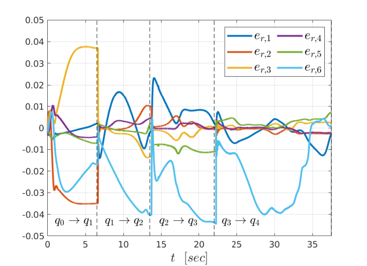

For comparison purposes, we also simulate a PID controller of the form
where , and are positive definite gain matrices. The errors , , for the four paths are shown in Fig. 104 (b). Note that they exceed the interval , which defined the clearance in the B-RRT algorithm, jeopardizing hence the actual trajectory of the robot. A video illustrating the robot trajectory using the two control laws can be found here: https://youtu.be/y7bCoUoTlPA.
24 Asymptotic Tracking of Nonsmooth Feedback Stabilizable Unknown Systems with Prescribed Transient Response
Finally, inspired by funnel-based techniques and the PPC methodology [115], we propose in this section a novel control scheme that achieves asymptotic stability while complying with funnel constraints, for a nd-order control affine uncertain and possibly non-smooth system.
24.1 Problem Formulation
We consider the asymptotic tracking control problem subject to transient constraints imposed by a predefined funnel. The consider systems are MIMO systems of the form
| (251a) | ||||
| (251b) | ||||
| (251c) | ||||
where , , with , , are the system’s states, is the system’s output, which is required to track a desired trajectory , and , are unknown vector fields, not necessarily continuous everywhere. We assume that is available for measurement, whereas is not. In fact, the dynamics governing is called dynamic uncertainty and represents unmodeled dynamic phenomena that potentially affect the closed-loop response. The assumptions on the system dynamics are restricted to local essential boundedness and measurability as well as controllability conditions on and internal stability of , without considering any uniform boundedness/growth condition or model approximation:
Assumption 6.3.
The maps , , are Lebesgue measurable and locally essentially bounded for each fixed , uniformly in , and the maps and are Lebesgue measurable and uniformly bounded for each fixed , by unknown bounds.
Assumption 6.4.
The matrix
is positive definite, , i.e., , where is its unknown minimum eigenvalue.
Assumption 6.5.
There exists a sufficiently smooth function and class functions , , such that , and
where is continuous and class for each fixed , and is uniformly bounded for each fixed .
Assumption 6.6.
The state is available for measurement.
Assumption 6.7.
The desired trajectory and its derivatives are bounded by finite and unknown constants , i.e., , , , where .
24.2 Problem Solution
The control objective is the asymptotic output tracking of a desired bounded trajectory , with bounded derivatives, as stated in Assumption 6.7. Moreover, as discussed before, we aim at imposing a certain predefined behavior for the transient response of the system. More specifically, motivated by funnel control techniques (Appendix 9, [359, 350, 352]), given predefined funnels, described by the smooth functions , where , are positive lower and upper bounds, respectively, we aim at guaranteeing that1111 11 The analysis can be extended to non-symmetric funnels. , , given that , . These functions can encode maximum overshoot or convergence rate properties. Note that, compared to the majority of the related works on funnel control (e.g., [372, 359, 352],[373]), we do not require arbitrarily small final values , which would achieve convergence of arbitrarily close to zero, since one of the objectives is actual asymptotic stability. In this section, the problem statement is as follows:
Problem 6.3.
Consider the system (251) and let a desired trajectory as well as prescribed funnels, described by , . Design a control protocol such that
- 1.
,
- 2.
, , ,
and all closed loop signals remain bounded.
Our solution to Problem 6.3 is based on the PPC error transformation, which converts the constrained error behavior to an unconstrained one. More specifically, we define the errors
| (252) |
as well as the error transformations according to:
| (253) |
where is a smooth, strictly increasing analytic function, with . Since is increasing, the inverse mapping is well-defined, and it holds that
| (254a) | |||
and hence, if remains bounded in a compact set, the desired funnel objective is achieved, . We further require that
| (255) |
A possible choice that satisfies the aforementioned specifications is .
From (253), we obtain
| (256) |
which, after differentiation, becomes
or, in stack vector form,
| (257) |
where , , , and . Due to the increasing property of , it holds that is positive definite, and thus in order to render negative a straightforward choice for a desired value for is
| (258) |
where is a positive and constant scalar gain. Since, however, is not the system’s input, we follow a backstepping-like methodology and define the error
| (259) |
Next, we proceed in a similar manner and define a funnel for each , , described by the functions , where are the positive lower and upper bounds, respectively, with the constraint , . Note that can be calculated at since it is a function of the state, the funnel functions and the desired trajectory profile. Then, we define the open set
| (260) |
and design the control law as
| (261) |
where
, , , , , are positive constant scalar gains, and is an adaptive variable gain, subject to the constraint , and dynamics
| (262) |
where is a positive constant gain.
Remark 6.4.
The control design procedure follows closely the prescribed performance backstepping-like methodology of Section 3.4, 7, introduced in [109]. The desired signals and control laws there consist only of proportional terms with respect to the transformed errors , , i.e., and in (258) and (261), respectively, which are guaranteed to be ultimately bounded. In this work, we incorporate (a) the extra terms in (258) that would render (257) exponentially stable, and (b) the discontinuous term in (261), which, as will be shown in the sequel, enforces convergence of the transformed errors to zero, guaranteeing thus asymptotic stability. This is achieved without requiring the funnel functions to converge to zero. However, one can still set the prescribed funnel to converge arbitrarily close to zero, achieving thus a predefined convergence rate.
Remark 6.5.
Note that no information regarding the dynamic model is incorporated in the control protocol (252)-(262). All the necessary signals consist of the funnel terms , and of known functions of the state and the desired trajectory . Furthermore, no a-priori gain tuning is needed and, as the next theorem states, the solution of Problem 6.3 is guaranteed from all initial conditions that satisfy , . As will be revealed subsequently, the adaptive gain compensates the unknown dynamic terms, which are proven to be bounded due to the confinement of the state in the prescribed funnels.
Theorem 6.3.
Consider a system subject to the dynamics (251), Assumptions 6.3-6.7, as well as a desired trajectory and funnels as described in Problem 6.3 satisfying , . Then the control protocol (252)-(262) guarantees the existence of at least one local Filippov solution of the closed-loop system (251)-(261) that solves Problem 6.3. Moreover, every such local solution can be extended to a global solution and all closed-loop signals remain bounded, for all .
Proof.
The intuition of the subsequent proof is as follows: We first show the existence of at least one Filippov solution of the closed loop system in for a time interval . Next, we prove that for any of these solutions, the state remains bounded in by bounds independent of the endpoint of . Hence, the dynamic terms of (251) are also upper bounded by a term, which we aim to compensate via the adaptation gain .
We start by defining some terms that will be used in the subsequent analysis:
Note that all the aforementioned terms are strictly positive. In particular, is strictly positive due to the definition of the funnels and Assumption 6.4, and is strictly positive due to the strictly increasing property of and hence of . Moreover, in view of (254), it holds that .
By employing (261), (262), we can write the closed loop system
| (263a) | ||||
| (263b) | ||||
| (263c) | ||||
| (263d) | ||||
where , , are the Filippov regularizations (see (270)) of the respective terms. For specifically, is formed by substituting the term with its reguralized term, which is if , and otherwise. Note that, in any case, it holds that . Define now and consider the open set . Since and , , the set is nonempty. Moreover, since , and hence its derivative, are analytic, their zero sets have zero measure [374] and thus the right hand-side of (263) is Lebesgue measurable and locally essentially bounded in over the set , and Lebesgue measurable in over the set . Hence, according to Prop. 8.1 of Appendix 8, for each initial condition , there exists at least one Filippov solution of (263), defined in , where such that , . By applying (256), we conclude the existence of the respective Filippov solutions , . Let now denote the initial condition of the system (263) satisfying and consider the family of Filippov solutions starting from denoted by the set . Note that, although not explicitly stated, and might be different for each solution in . We aim to prove that all are bounded and converge to zero, for all .
In view of the definition of (see also (260)), for all it holds that
| (264a) | ||||
| (264b) | ||||
, where and are the upper bounds of and , respectively, . Consider now the Lyapunov function , for which it holds, in view of (257), (258), (259), and (264b)
. Hence, we conclude that when . Since is positive definite, , the latter is equivalent to . Hence, we conclude that all satisfy
Since is finite, it holds that and hence , . Moreover, since and are smooth, the derivative approaches infinity only when . Therefore, in view of the definition of in (257), we conclude the existence of a finite such that , . Next, (253) implies that , . Hence, we conclude that , , where is the uniform bound of the desired trajectory, introduced in Assumption 6.7. We also conclude that , . In addition, by employing and (264b), we conclude that , . Finally, by differentiating , employing the smoothness and boundedness of and its derivatives, the smoothness of , the boundedness of as well as the aforementioned bounds, we can conclude the existence of a bound such that , .
Furthermore, the boundedness of and Assumption 6.5 imply the existence of a positive finite constant such that , . Hence, since is Lebesgue measurable and locally essentially bounded in and , , , , there exists some positive , such that , , and hence, for each , since is formed by the convex closure of , it holds that , and . Note that, in view of the aforementioned discussion, depends solely on the initial conditions and the parameters of the funnel functions. Define now the finite constant term as
| (265) |
Note that the term in the parenthesis of (265) is an upper bound for the term , for all and almost all .
Define also the signal , where is the adaptive gain introduced in (261). Consider now the function
where , and is a positive constant to be defined; satisfies , for and . Then, according to Lemma 8.2 of Appendix 8, with
Since is continuously differentiable, its generalized gradient reduces to the standard gradient and thus it holds that , where . After using (251), (261), (262), and , one obtains
Note that, since , (262) implies that , . Moreover, since the Filippov regularization (270) is defined as a closed set and , it holds that . By substituting and employing the skew-symmetry of the second term, we obtain in view of Assumption 6.4 and the definition of in (265):
for all solutions . By setting in (255), we obtain and hence by employing , , we obtain that
Therefore, by setting , employing , and in view of the fact that , we obtain
, , where is continuous and positive semi-definite on , since and are positive definite. Hence, we conclude that , , and all . Choose now any finite and let . Note that all the conditions of Theorem 8.6 in Appendix 8 are satisfied and hence, all Filippov solutions starting from are bounded and remain in , . Moreover, , implying that and it also holds that and , which, in view of the increasing property of and the fact that , implies that and . Notice that Zeno behavior is avoided since .
Note that , and hence , can be arbitrarily large allowing any finite initial condition , which implies any . In addition, it holds that , which implies the boundedness of , and by . Therefore, we conclude that , . Moreover, by employing (253), we conclude that , and hence , . Therefore, we conclude that all solutions are bounded in compact sets , which means that , and , as designed in (261) and (262), respectively, remain also bounded, . ∎
Remark 6.6.
Note that no boundedness assumptions or growth conditions are needed for the vector fields and . In particular, the effect of is canceled by the introduced adaptive signal , which increases according to (262). It is proved, nevertheless, that this adaptive signal remains bounded. Moreover, the response of the system is solely determined by the funnel functions and , isolated from the system dynamics and the control gains selection. Nevertheless, we note that appropriate gain tuning might be needed to suppress chattering in real life scenarios. Similarly, note that the region of attraction (initial conditions) of is independent from the system dynamics and the control gain selection and depends only on the choice of the funnel functions , . In particular, if are design parameters, we can always choose them such that , , which renders the result global. In fact, the choice , [352] is not excluded from our control scheme and does not restrict the initial condition . Moreover, noise can be taken into account in the measurement of , i.e., consider that is available for measurement, where is an unknown noise signal with appropriate continuity and boundedness properties. By redefining and including the time derivative of in (265), the analysis still holds. Note, however, that in this case it can only be deduced that and hence does not necessarily converge to .
Remark 6.7.
Since funnel control traditionally guarantees confinement of the state in the desired funnel, a common practice is to tune the funnel to converge to arbitrarily small values, achieving thus “practical stability”, i.e., the state converging arbitrarily close to zero. Note that, in our case, the funnel functions , , are not required to decrease to values arbitrarily close to zero, yet asymptotic stability is still achieved. In fact, the proposed control schemes can be used to achieve merely asymptotic stability results without any funnel constraints, if the latter is not required. More specifically, given the initial errors , we can use the proposed control protocols by employing any constant values , . Finally, the proposed control scheme can be extended to systems of the form for some , where the funnel constraints are set for the combined signal .
24.3 Simulation Results
We consider here the simulation of two inverted pendulum connected by a spring and a damper [372], with dynamics:
where is the force between the connection points of the spring and damper at the pendulums, and
is the distance between these connection points; is defined as
and , are friction terms on the motors evolving according to , with
The time varying signal is taken as:
modeling a loss of effectiveness of the second motor when . We also choose as the gravity constant and , . The initial conditions are , (rad, rad/s), and the desired trajectory rad. The prescribed funnel functions are chosen as , , which converge to . We also choose , as well as the gains , , , , , and . The simulation results are depicted in Figs. 105-108 for . More specifically, Fig. 105 depicts the errors along with the performance functions , . One can conclude that and not only respect their imposed funnels but also converge asymptotically to zero, without the need of arbitrarily small values for and . This can be verified also by Fig. 106, which depicts the evolution of the transformed errors , , , and shows their asymptotic convergence to zero. Finally, Figs. 107 and 108 illustrate the inputs as well as the adaptation signal , . One can conclude the convergence of to a constant value as well as the boundedness of the control input , as was proved in the theoretical analysis.
25 Conclusion
This chapter presented planning and control algorithms for single-agent systems. Firstly, we developed a hybrid algorithm for the planning of a robotic system under timed temporal logic formulas in an obstacle-cluttered workspace. By using previous results, we guaranteed the collision-free timed navigation leading to a timed abstraction of the system. A high-level planner and a novel optimization technique provided the timed path that satisfy the specification and is asymptotically optimal via reconfiguration. Secondly, we turned our attention to the motion planning of high-dimensional uncertain systems (e.g., robotic manipulators). We developed a two-layer framework by integrating adaptive control techniques and sampling-based motion planning. The closed-loop system provably navigated to a desired goal while avoiding collisions and compensating for the dynamic uncertainties. Finally, we developed a control scheme that guarantees asymptotic stability for an uncertain nd-order system, while complying to funnel constraints, by integrating adaptive and discontinuous control methodologies.
Chapter 7 Summary and Future Research Directions
This chapter summarizes the content of the thesis and provides potential future research directions.
26 Summary
In Chapter 2, we proposed a set of control algorithms for the cooperative manipulation of rigid objects. We tackled first the case of rigid grasping contacts, and developed closed-form adaptive control algorithms, compensating for uncertainty in the dynamic parameters of the object and the agents, and Nonlinear Model Predictive Control schemes, taking into account constraints such as obstacle avoidance and input saturation. A Prescribed Performance Control methodology has been also developed to achieve prescribed transient and steady-state response for the object. Secondly, we considered the case of rolling contacts, for which we developed novel centralized and decentralized control algorithms that guarantee agents-object contact maintenance, along with object reference tracking.
In Chapter 3, we tackled the problem of multi-agent formation and its relation to rigid cooperative manipulation. Firstly, we developed a robust model-free decentralized control scheme for the formation control of a tree-graph multi-agent system with prescribed transient and steady-state response, subject to collision and connectivity constraints. Secondly, we associated rigid cooperative manipulation schemes to multi-agent rigidity theory. We related the grasp matrix of the former to the rigidity matrix of the latter and we used that to derive novel conditions for the internal force-free cooperative manipulation.
In Chapter 4 we considered the problems of multi-agent navigation and leader-follower coordination subject to collision and/or connectivity constraints as well as uncertain dynamics. We first developed an adaptive control protocol for the problem of single-agent navigation in an obstacle-cluttered environment with uncertain dynamics under almost all initial conditions. This was extended to a prioritization-based decentralized scheme for multi-agent systems. Secondly, we proposed a novel adaptive control scheme for the leader-follower coordination, that is, navigation of a leader agent to a predefined pose, while guaranteeing collision avoidance and connectivity maintenance. Finally, we designed an adaptive control protocol for the collision avoidance among ellipsoidal agents using a novel distance metric for D ellipsoids.
In Chapter 5 we used previous continuous control schemes to derive appropriate discrete abstractions and synthesize controllers for the satisfaction of complex tasks expressed as temporal logic formulas. We first considered local tasks for multi-agent systems, such as UAVs and robotic manipulators, and then we focused on cases where unactuated objects have their own specifications. We considered discretizations both using predefined regions of interest as well as a full workspace partition. Collision avoidance was taken into account to define safe transitions among the discrete states. Linear and Metric Interval Temporal Logic formulas were applied and control synthesis was performed using standard automata-based formal verification techniques.
In Chapter 6 we developed extension algorithms for single-agent problems. Firstly, we considered the motion planning problem of a single agent in an obstacle-cluttered environment under timed temporal tasks. By using previous results on safe timed navigation, we developed an algorithm that guarantees the satisfaction of the timed specification as well as asymptotically optimal performance in terms of energy efficiency. Secondly, we addressed the problem of motion planning of high-dimensional complex systems in obstacle-cluttered environments with uncertain dynamics. We integrated adaptive control techniques with sampling-based motion planning algorithms to develop a two-layer framework that guarantees the safe navigation of the system to its goal. Finally, we developed a novel model-free adaptive control scheme that guarantees asymptotic stability of a class of nonlinear systems while respecting predefined funnel constraints.
27 Future Research Directions
Regarding the cooperative manipulation schemes of Chapter 2, a strong assumption is that the agents operate away from kinematic singularities (except for the NMPC frameworks). Future directions can aim at addressing this issue and guarantee singularity avoidance. Moreover, grasp reconfiguration that allows more modular schemes is a promising direction, as well as fault-tolerant extensions of the current schemes. Finally, real-time experiments with robotic agents with soft fingertip-type end-effectors should be attempted.
Regarding Chapter 3, future efforts can aim at extending the developed formation control scheme to more general multi-agent graph structures as well as taking into account collisions among all the agents. Moreover, one can notice that the control law for provably achieving zero internal forces in the rigid cooperative manipulation scheme, depending on the multi-agent rigidity matrix, is centralized. Therefore, one might aim at extending the proposed algorithm to a decentralized scheme as well as considering compliant grasping contacts. Real-time experiments should be also conducted to showcase the validity of the proposed conditions.
Regarding the multi-agent coordination of Chapter 4, future works can address less conservative solutions for the multi-agent collision-free navigation. This can be also attempted by using the proposed leader-follower scheme and appropriate prioritization. Sampled inter-agent communication should be also used to resemble more realistic scenarios. Regarding the proposed ellipsoidal collision avoidance problem, one drawback that is required to be tackled in future works is the fact that the scheme interferes with the main assigned tasks, potentially causing them to fail (local minima scenarios).
Regarding Chapter 5, future directions are needed towards the generalization of the proposed multi-agent schemes to incorporate timed temporal specifications. Regarding the multi-agent-object hybrid scheme that is based on region-of-interest discretization, a decentralized extension must be considered. Moreover, failure of transition executions can be taken into account via plan reconfiguration. Finally, future works should also focus on real-time experiments to further validate the proposed frameworks.
Finally, regarding Chapter 6, future works are required to focus mainly at extending the proposed frameworks to multi-agent schemes, as well as incorporation of input saturation constraints.
As a final remark, another interesting topic of research is the consideration of delays in the multi-agent communication, as well as the sampled feedback and control realization, which have been neglected in this thesis.
Appendix 8 Dynamical Systems
This Appendix provides preliminary background on the theory of dynamical systems. We consider both smooth and non-smooth systems.
Appendix 8.A Lipschitz Continuous Systems
We start with defining standard results on the existence of solutions of ODEs.
Consider the initial value problem:
| (266) |
with where is a non-empty open set containing the origin, and .
Definition 8.1.
Theorem 8.1.
[376] Let from (266) satisfy the following conditions:
- 1.
For every , the function defined on is measurable. For every , the function defined on is continuous.
- 2.
For every compact , there exist constants such that
.
Then the initial value problem (266) with and some , has a unique and maximal solution , with and .
Note that the second condition imposed in the aforementioned theorem is a locally Lipschitz condition.
Theorem 8.2.
Definition 8.2.
The origin is the equilibrium point for (266) if
We next provide the comparison function definitions, necessary for the stability classification of the equilibrium point.
Definition 8.3.
Definition 8.4.
Now we can characterize the equilibrium point of (266) with respect to its stability.
Definition 8.5.
([319, 12]) The equilibrium point of (266) is
- •
uniformly stable, if there exists a class function and a positive constant independent of , such that
(267) - •
uniformly asymptotically stable, if there exists a class function and a positive constant independent of , such that
(268) - •
exponentially stable, if (268) is satisfied with , ,
- •
globally uniformly stable, if (267) is satisfied with for any initial state and ,
- •
globally uniformly asymptotically stable, if (268) is satisfied with for any initial state ,
- •
globally exponentially stable, if (268) is satisfied for any initial state and with , .
The main Lyapunov stability theorem is then formulated as follows:
Theorem 8.3.
([319, 12]) Let be an equilibrium point of (266). Let be a continuously differentiable function such that, , ,
Let such that . Then, the equilibrium point of (266) is
- •
uniformly stable, if and are class functions on and on ,
- •
uniformly asymptotically stable, if , , and are class functions on ,
- •
exponentially stable, if on , , ,
- •
globally uniformly stable, if , and are class functions, and on ,
- •
globally uniformly asymptotically stable if , and are class functions, and is a class function on ,
- •
globally exponentially stable, if , on , , ,
We provide next standard invariance results for time-invariant and time-varying systems.
Theorem 8.4.
(LaSalle [319, 12]) Let be a positive invariant non-empty set of the time-invariant ODE , where is continuous and satisfies condition 2 of Theorem (8.1). Let be a continuously differentiable function such that , . Let , and let be the largest invariant set contained in . Then, every bounded solution starting in converges to as .
Lemma 8.1.
We conclude the results for smooth systems with the standard ultimate boundedness theorem.
Theorem 8.5.
([319, 12]) Let be an equilibrium point of (266). Let be a continuously differentiable function such that
, , where , are class functions and is a continuous positive definite function. Take such that and suppose that . Then, there exist a class function and for every initial state satisfying , there exists a such that
Moreover, if and belongs to class , then the aforementioned result holds for any initial state , with no restriction on how large is.
Note that the aforementioned results also apply for the case where evolves in a manifold, by changing the metric to the respective manifold one.
Appendix 8.B Systems with Discontinuous Right-Hand-Side
This section provides some equivalent results for non-smooth systems.
Consider the following differential equation with a discontinuous right-hand side:
| (269) |
where , , is Lebesgue measurable and locally essentially bounded, uniformly in . The Filippov regularization of is defined as [377]
| (270) |
where is the intersection over all sets of Lebesgue measure zero, and is the convex closure of a set . We are interested in the Filippov solutions of (269):
Definition 8.6 ([378]).
A function , with , is called a Filippov solution of (269) on if is absolutely continuous and if, for almost all , it satisfies , where is the Filippov regularization of .
The existence of Filippov solutions is given next.
Proposition 8.1 ([379]).
Let , where is the Filippov regularization of . Let also be measurable and locally essentially bounded in over , and measurable in over . Then, there exists a Fillipov solution of (269).
We next provide the definitions for regular functions and generalized gradients.
Definition 8.7 ([378]).
Given a function , the right directional derivative of at in the direction of is defined as
Additionally, the generalized directional derivative of at in the direction of is defined as
Definition 8.8 ([378]).
A function is said to be regular at if for all , the right directional derivative of at in the direction of exists and .
Definition 8.9 ([378]).
For a function that is locally Lipschitz in , define the generalized gradient of at by
where is the set of measure zero where the gradient of is not defined.
Lemma 8.2 ([378]).
Let be a Filippov solution of (269) and be a locally Lipschitz, regular function. Then is absolutely continuous, exists almost everywhere (a.e.), i.e., for almost all , and , where
Finally, we provide the main invariance and stability result for the non-smooth type (269).
Theorem 8.6 ([378]).
For the system given in (269), let be an open and connected set containing and suppose that is Lebesgue measurable and is essentially locally bounded, uniformly in . Let be locally Lipschitz and regular such that , , , and
where and are continuous positive definite functions and is a continuous positive semi-definite on . Choose and such that and . Then for all Filippov solutions of (269), with , it holds that , , , and .
Appendix 8.C Reduction Principle
Consider now the autonomous time-invariant version of (266)
| (271) |
where is sufficiently smooth, and is an equilibrium point, i.e., . Let be the respective Jacobian matrix with eigenvalues with positive real part, eigenvalues with negative real part, and eigenvalues with zero real part. Let denote the linear (generalized) eigenspace of corresponding to the union of the eigenvalues on the imaginary axis. The next theorem provides the center manifold existence around the equilibrium point.
Theorem 8.7 ([380]).
There is a locally defined smooth -dimensional invariant manifold of (271) that is tangent to at .
System (271) can be written as
| (272a) | |||
| (272b) | |||
where , , is a matrix with all its eigenvalues on the imaginary axis, while has no eigenvalue on the imaginary axis. The functions and have Taylor expansions starting with at least quadratic terms. The center manifold of system (272) can be locally represented as a graph of a smooth function as .
Appendix 9 Funnel Control
This Appendix provides preliminary background on funnel control and in particular, Prescribed Performance Control (PPC).
Funnel control describes the behavior where the output of the system is confined to a predefined funnel, as depicted in Fig. 109. A special instance of funnel control, which this thesis focuses on, is Prescribed Performance Control, proposed in [115], and describes the behavior where a tracking error , with , evolves strictly within a predefined region that is bounded by certain functions of time, achieving prescribed transient and steady-state performance. The mathematical expression of prescribed performance is given by the inequalities:
where are smooth and bounded functions of time satisfying and , called performance functions.
Although the functions can be any bounded functions, it is usually preferred to be decaying functions. A particular interesting instance is the choice of the exponential performance functions , with , appropriately chosen constants, the terms are selected such that and the terms represent the maximum allowable size of the tracking error at steady state, which may be set arbitrarily small to a value reflecting the resolution of the measurement device, thus achieving practical convergence of to zero. Moreover, the decreasing rate of , which is affected by the constants in this case, introduces a lower bound on the required speed of convergence of . Therefore, the appropriate selection of the performance functions imposes performance characteristics on the tracking error .
The systems considered are general nonlinear systems of the form
where are unknown functions satisfying certain continuity and controllability properties. We describe briefly the control design as well as the intuition behind it. Firstly, given a desired signal and an error , as well as a choice of performance functions , for each component , we define the normalized error
where , as well as the transformation , with
Intuitively, in order to guarantee , we need to guarantee that is bounded. This is attempted via the choice of control law
which acts as a barrier function, i.e., it increases to infinity as approaches the boundary of . Local existence of solutions guarantees that there exists a maximal time such that , . Differentiating thus the well-defined (for ) Lyapunov function candidate yields
By assuming Lipschitz , uniform bounded , and positive definite , we use the boundedness of , to conclude that the second term above is bounded by a constant , . Hence it turns out that when , from which we can conclude the ultimate boundedness of in a compact set, and hence that .
Appendix 10 Navigation Functions
This Appendix provides preliminary background on navigation functions.
Navigation functions, initially proposed in [313] for single-point-sized robot navigation, are real-valued maps realized through cost functions, whose negated gradient field is attractive towards the goal configuration (referred to as the good or desirable set) and repulsive with respect to the obstacles set (referred to as the bad set which we want to avoid). We provide here a brief overview of the multi-agent versions introduced in [314] and [309].
Appendix 10.A Multirobot Navigation Functions (MRNFs)
Consider spherical robots, with center , , and radius , i.e., , , operating in an open spherical workspace of radius . Each robot has a destination point , and . Let be a compact connected analytic manifold with boundary. A map is a Multirobot Navigation Function (MRNF) if
- 1.
It is analytic on ,
- 2.
It has only one minimum at ,
- 3.
Its Hessian at all critical points is full rank,
- 4.
, ,
where . The class of MRNFs has the form
where is the goal function, is the obstacle function, and is a tunable gain; denotes the desirable set and the set we want to avoid. Next we provide the procedure for the construction of the function .
A robot proximity function, a measure for the distance between two robots , is defined as , . The term relation is used to describe the possible collision schemes that can be defined in a multirobot team, possibly including obstacles. The set of relations between the members of the team can be defined as the set of all possible collision schemes between the members of the team. A binary relation is a relation between two robots. Any relation can be expressed as a set of binary relations. A relation tree is the set of robot/obstacles that form a linked team. Each relation may consist of more than one relation tree. The number of binary relations in a relation is called relation level. Illustrative examples can be found in [314]. A relation proximity function (RPF) provides a measure of the distance between the robots involved in a relation. Each relation has its own RPF. A RPF is the sum of the robot proximity functions of a relation. It assumes the value of zero whenever the related robots collide (since the involved robot proximity functions will be zero) and increases with respect to the distance of the related robots. The RPF of relation at level is given by , where we omit the arguments for notational brevity. A relation verification function (RVF) is defined as
where , and is the complementary to set of relations in the same level , is an index number defining the relation in level , and . The RVF serves as an analytic switch, which goes to zero only when the relation it represents is realized. By further introducing the workspace boundary obstacle functions as , we can define where is the number of levels and the number of relations in level . It has been proved that, by choosing the parameter large enough, the negated gradient field leads to the destination configuration , from almost all initial conditions [314].
Appendix 10.B Decentralized Navigation Functions (DNFs)
Consider now the class of decentralized navigation functions, which has the form , with . The key difference in this case is the term that is associated with the collision avoidance property of agent with the rest of the team and is based on the inter-agent decentralized distance function [309]: with
that represents the distance between agents and . The term is used in order to avoid inter-agent collisions in case one or more agents that take part in a collision scheme are very close to their goals. Note that in that case, the classical form of would yield values very close to , since agent is very close to its goal, without actively taking part in avoiding potential collisions. The term , therefore, forces agent to avoid potential collisions. Analytic expressions for and can be found in [309]. With the aforementioned tools, the control law for agent is , which, as shown in [309], drives all agents to their goal positions and guarantees inter-agent collision-avoidance.
Appendix 11 Nonlinear Model Predictive Control
This Appendix provides preliminary background on Nonlinear Model Predictive Control (NMPC).
Nonlinear Model Predictive Control has become an attractive feedback control strategy in applications where, except for stabilization or trajectory tracking of a system, certain state and input constraints must be also satisfied [381, 88, 87]. In general, the NMPC is formulated as solving at each sampling time step an online Finite Horizon Optimal Control Problem (FHOCP) subject to system dynamics and state and input constraints. Based on measurements obtained at each sampling time step, the controller predicts the dynamic behavior of the system over a predictive horizon in the future and determines the input such that a predetermined open-loop performance objective is minimized. In order to incorporate feedback, the optimal open-loop input is implemented only until the next sampling time step. Using the new system state at the next sampling time step, the whole procedure (prediction and optimization) is repeated, moving the control and prediction horizon forward. Summarizing, a standard NMPC scheme works as follows
- 1.
Obtain estimates of the states of the system.
- 2.
Calculate a constraint-conforming optimal input minimizing the desired cost function over the prediction horizon using the system model and the current state estimate for prediction.
- 3.
Implement the first part of the optimal input until the next sampling time step.
- 4.
Go to step 1.
More technically, consider the stabilization problem for a class of systems described by the following nonlinear dynamical system:
| (273) |
with is locally Lipschitz continuous and satisfies . The system is subject to the following input and state constraints:
respectively, where is compact and is connected, and . Denote by , the sampling step and the finite prediction horizon, respectively. Consider a sequence of sampling times . Then, at every sampling time step , the following FHOCP is solved:
| (274a) | ||||
| subject to: | (274b) | |||
| (274c) | ||||
| (274d) | ||||
| (274e) | ||||
where and are running and terminal costs, respectively, usually chosen as
?where and are positive definite matrix and a positive semi-definite weight matrix. The hat denotes predicted variables (internal to the controller), i.e., is the solution of (274) driven by the input with the initial condition . Due to the fact that a finite prediction horizon is used, the actual closed-loop input and state trajectories will differ from the predicted open-loop trajectories, even if no model plant mismatch and no disturbances are present. This is the key difference between standard control strategies, where the feedback control law is obtained a priori, and NMPC, where the feedback control law is obtained online. Since a finite horizon approach is used, the terminal set is introduced and is appropriately designed as described in [381, 88] in order to guarantee the stability of the closed-loop system. The solution to FHOCP (274) is denoted by . It defines the open-loop input that is applied to the system until the next sampling time step as
The control input is a feedback control law, since it is re-calculated at each sampling instant using the new state information. The solution of (273) from an initial state , applying an input is denoted by , . We next define the admissible control input.
Definition 11.1.
A control input for a state is called admissible, if
- 1.
it is piecewise continuous;
- 2.
;
- 3.
;
- 4.
;
The following theorem states the stability results for NMPC.
Theorem 11.1 ([87]).
Consider system (273) and suppose that
- •
the NMPC open-loop optimal control problem (274) is feasible at
- •
the terminal set is closed with and the terminal cost is cont. differentiable and positive definite
- •
the terminal set and terminal cost are chosen such that, , there exists an (admissible) input such that , , and
Then, the closed-loop system is asymptotically stable with the region of attraction being the sets of states for which the an admissible input exists.
Appendix 12 Graph Theory and Rigid Frameworks
This Appendix provides preliminary background on graph theory and rigid frameworks.
Appendix 12.A Graph Theory
An undirected graph is a pair , where is a finite set of nodes, representing a team of agents, and , with , is the set of edges that model the communication capabilities between neighboring agents. For each agent, its neighboring set is defined as . A directed graph is formed by the edges being , i.e., does not necessarily imply . The complete graph of nodes, , is denoted by .
If there is an edge , then are called adjacent. A path of length from vertex to vertex is a sequence of distinct vertices, starting with and ending with , such that consecutive vertices are adjacent. For , the path is called a cycle. If there is a path between any two vertices of the graph , then is called connected. A connected graph is called a tree if it contains no cycles.
Consider an arbitrary orientation of , which assigns to each edge precisely one of the ordered pairs or . When selecting the pair , we say that is the tail and is the head of the edge . By considering a numbering of the graph’s edge set, we define the incidence matrix as
Moreover, the incidence matrix satisfies the following important property.
Property 12.1.
Consider the incidence matrix of an arbitrary graph as , where are the rows of . Then it holds that , i.e., the rows of the incidence matrix sum up to zero.
Lemma 12.1.
[128, Section III] Assume that the graph is a connected tree. Then, is positive definite for any positive definite matrix .
Appendix 12.B Rigidity Theory
We review here some necessary notions on distance and bearing rigidity.
12.B.1 Distance Rigidity in
Let an undirected graph and be the position of node . Let also . A framework in is the tuple . We assume that the nodes are not collinear in or occupy the exact same position.
Definition 12.1.
Two frameworks and are distance equivalent if , .
Definition 12.2.
Two frameworks and are distance congruent if , .
Definition 12.3.
A framework is distance rigid if there exists a constant such that any framework that is distance equivalent to and satisfies is also distance congruent to it.
Definition 12.4.
A framework is globally distance rigid if an arbitrary framework that is distance equivalent to is also distance congruent to it.
Consider an orientation assigned to , as described in the previous section, as well as a numbering , . Let the interneighbor distances be expressed by , . Define the distance function as
The distance rigidity matrix is defined as the respective Jacobian
Let now be a variation of the configuration . If , then is an infinitesimal distance motion of . An infinitesimal distance motion is trivial if it corresponds only to a translation and a rotation of the entire framework.
Definition 12.5.
A framework is infinitesimally rigid if all the infinitesimal distance motions are trivial.
Lemma 12.2.
A framework is infinitesimally rigid if
- •
, if
- •
, if
12.B.2 Bearing Rigidity in
Let a directed graph and now be the pose of node . Let also . A framework in is the tuple . We assume that the nodes are not collinear in or occupy the exact same position.
Let be the relative bearings, with
as well as .
Definition 12.6.
Two frameworks and are bearing equivalent if
Definition 12.7.
Two frameworks and are bearing congruent if
Definition 12.8.
A framework is globally bearing rigid in if every framework which is equivalent to it is also congruent to it.
Definition 12.9.
A framework is bearing rigid in if there exists a neighborhood of such that
Similar to distance rigidity, the respective rigidity matrix is defined as , whose null-space describes the infinitesimal bearing motions of in . An infinitesimal bearing motion in is trivial if it corresponds only to a translation, rotation, or dilation of the framework. The infinitesimal bearing rigidity in follows from Definition 12.5.
Lemma 12.3.
A framework is infinitesimally bearing rigid in if and only if , or, equivalently, .
Appendix 13 Temporal Logics-based Task Specification
This Appendix provides preliminary background on specifications expressed as temporal logic formulas.
Appendix 13.A Task Specification in LTL
Definition 13.1.
A transition system () is a tuple ), where is a discrete finite set of states, is a discrete finite set of initial states, is a transition relation, is a discrete set of atomic propositions1212 12 boolean variables that are either true or false in a given state, and is a labeling function that assigns to each state the atomic propositions that are true in that state.
Definition 13.2.
A run of a is an infinite sequence
with , , .
Definition 13.3.
A word of a run is the infinite sequence
where .
We focus on the task specification given as a Linear Temporal Logic (LTL) formula. The basic ingredients of a LTL formula are a set of atomic propositions and several boolean and temporal operators. LTL formulas are formed according to the following grammar [260]: , where , and are LTL formulas and , are the next and until operators, respectively. Definitions of other useful operators like (always), (eventually) and (implication) are omitted and can be found at [260]. The semantics of LTL are defined over infinite words over . Intuitively, an atomic proposition is satisfied on a word if it holds at its first position , i.e. , denoted as . Formula holds true if is satisfied on the word suffix that begins in the next position , whereas states that has to be true until becomes true. Finally, and holds on eventually and always, respectively. For a full definition of the LTL semantics, the reader is referred to [260].
A LTL formula over a set of atomic propositions can be translated to a Büchi Automaton [260]. Then, by calculating the product of the transition system with as , we can find the runs of that satisfy the formula . These runs can then be projected back to , providing paths over that satisfy . More details regarding the technique can be found in [260].
Appendix 13.B Task Specification in MITL
Definition 13.4.
A Weighted Transition System () is a tuple
where is a discrete finite set of states, is a discrete finite set of initial states, is a transition relation, is a finite set of atomic propositions, is a labeling function and is a map that assigns a positive weight to each transition.
Definition 13.5.
[305] The time sequence is an infinite sequence of time values , satisfying the following constraints:
- •
Monotonicity: .
- •
Progress: such that .
Definition 13.6.
Let be a finite set of atomic propositions. A timed word over is an infinite sequence
where is an infinite word over and is a time sequence according to Definition 13.5.
Definition 13.7.
A timed run of a is an infinite sequence
such that , and . The time stamps are inductively defined as
- 1.
,
- 2.
.
The timed run generates the timed word
over the set , where is the subset of atomic propositions that are true at state at time , .
The syntax of Metric Interval Temporal Logic (MITL) over a set of atomic propositions is defined by the grammar
where , and and are the next, future, always and until operators, respectively; is a nonempty time interval in one of the following forms: with . MITL can be interpreted either in continuous or point-wise semantics. We utilize the latter and interpret MITL formulas over timed runs such as the ones produced by a .
Definition 13.8.
We provide next a description of Timed Büchi Automata (TBA), originally proposed in [305]. Let be a finite set of clocks. The set of clock constraints is defined by the grammar:
where is a clock, is a clock constraint, and . A clock valuation is a mapping that assigns a value to each clock. A clock has valuation for . Given and , we denote by and the fact that the valuation and the time instant , respectively, satisfy the clock constraint .
Definition 13.9.
A Timed Büchi Automaton is a tuple
where is a finite set of locations, is the set of initial locations, is a finite set of clocks, is a finite set of atomic propositions that defines the input alphabet , gives the set of edges of the form , where , are the source and target locations, is the guard of edge, is a set of clocks to be reset upon executing the edge, and is an input string; finally, is a set of accepting locations.
A state of is a pair . The initial state of is , with . Given two states , , and an edge , there exists a discrete transition if . Moreover, , , and , . Given , there exists a time transition if and (component-wise summation). We write if there exists such that and , with .
An infinite run of starting at a state is an infinite sequence of time and discrete transitions , where , . This run corresponds to the timed word , with , . The run is called accepting if for infinitely many . A timed word is called accepting if there exists an accepting run associated with it. The problem of deciding the language emptiness of a given TBA is PSPACE-complete [305]. In other words, an accepting run of a given TBA can be synthesized, if one exists. Any timed formula over originating from the decidable fragment of timed logics (e.g., MITL, discrete-time MTL, finite MTL1313 13 In this case, the generated Timed Automaton will have finite accepting runs., coFlat-MTL, Bounded-MTL [382, 383]) can be algorithmically translated into a TBA with input alphabet , such that the language of timed words that satisfy is the language of timed words produced by the TBA.
Appendix 14 Useful Properties
This appendix provides some additional technical properties that are useful throughout the thesis.
Proposition 14.1.
Let , with . Then it holds that , .
Proof.
It holds that . Hence, , . ∎
Proposition 14.2.
[169] Let , and . Then .
Proposition 14.3.
Let . Then, for the rotation matrix it holds that ; if and only if ; when , for every in the unit sphere.
Let , , and . Then the following hold [170]:
- •
;
- •
;
- •
;
- •
.
We provide next some useful properties of linear algebra.
Definition 14.1.
A matrix is left equivalent (or row equivalent) to a matrix if and only if there exists an invertible matrix such that .
The following propositions can be proved:
Proposition 14.4.
Let Then and are left equivalent if and only if they have the same nullspace , i.e., , for any .
Proposition 14.5.
Let , and , where is an invertible matrix. Then it holds that
Proposition 14.6.
Let such that . Then it holds that
Proposition 14.7.
Consider the cubic equation with and roots , with . Then, given its discriminant , the following hold:
- (i)
, with , such that , i.e., at least two roots are equal,
- (ii)
, and , with , i.e., all roots are real and distinct.
Proposition 14.8.
[384] Consider two planar ellipsoids
with , , and terms that describe their motion in D space. Given their characteristic polynomial , which has degree , the following hold:
- (i)
, i.e, the polynomial has always one positive real root,
- (ii)
if and only if the characteristic equation has two distinct negative roots, i.e., , with , and .
- (iii)
and , i.e., and touch externally, if and only if and only if has a negative root with multiplicity .
Index
References
- [1] W. Ren and R. Beard. Consensus Seeking in Multi-agent Systems under Dynamically Changing Interaction Topologies. IEEE Transactions on Automatic Control (TAC), 50(5):655–661, 2005.
- [2] R. Olfati-Saber and R. Murray. Consensus problems in networks of agents with switching topology and time-delays. IEEE Transactions on Automatic Control (TAC), 49(9):1520–1533, 2004.
- [3] A. Jadbabaie, J. Lin, and S. Morse. Coordination of groups of mobile autonomous agents using nearest neighbor rules. IEEE Transactions on Automatic Control (TAC), 48(6):988–1001, 2003.
- [4] H. Tanner, A. Jadbabaie, and G. J. Pappas. Flocking in fixed and switching networks. IEEE Transactions on Automatic Control (TAC), 52(5):863–868, 2007.
- [5] D. V. Dimarogonas and K. Kyriakopoulos. On the rendezvous problem for multiple nonholonomic agents. IEEE Transactions on Automatic Control (TAC), 52(5):916–922, 2007.
- [6] M. Egerstedt and X. Hu. Formation constrained multi-agent control. IEEE Transactions on Robotics and Automation, 17(6):947–951, 2001.
- [7] K. Oh, M. Park, and H. Ahn. A survey of multi-agent formation control. Automatica, 53:424–440, 2015.
- [8] M. Ji and M. Egerstedt. Distributed Coordination Control of Multi-Agent Systems While Preserving Connectedness. IEEE Transactions on Robotics (TRO), 23(4):693–703, 2007.
- [9] M. Zavlanos and G. J. Pappas. Potential Fields for Maintaining Connectivity of Mobile Networks. IEEE Transactions on Robotics (TRO), 23(4):812–816, 2007.
- [10] M. Zavlanos and G. J. Pappas. Distributed connectivity control of mobile networks. IEEE Transactions on Robotics (TRO), 24(6):1416–1428, 2008.
- [11] D. V. Dimarogonas, S. G. Loizou, K. J. Kyriakopoulos, and M. Zavlanos. A Feedback Stabilization and Collision Avoidance Scheme for Multiple Independent Non-Point Agents. Automatica, 42(2):229–243, 2006.
- [12] M. Krstic, I. Kanellakopoulos, and P. Kokotovic. Nonlinear and Adaptive Control Design. Publisher: Wiley New York, 1995.
- [13] Christos K Verginis, Matteo Mastellaro, and Dimos V Dimarogonas. Robust quaternion-based cooperative manipulation without force/torque information. IFAC-PapersOnLine, 50(1):1754–1759, 2017.
- [14] Christos K Verginis, Matteo Mastellaro, and Dimos V Dimarogonas. Robust cooperative manipulation without force/torque measurements: Control design and experiments. IEEE Transactions on Control Systems Technology, 28(3):713–729, 2020.
- [15] A. Nikou, C. K. Verginis, S. Heshmati-alamdari, and D. V. Dimarogonas. A nonlinear model predictive control scheme for cooperative manipulation with singularity and collision avoidance. Proceedings of the 25th IEEE Mediterranean Conference on Control and Automation (MED), Valletta, Malata, pages 707–712, 2017.
- [16] Christos K Verginis, Alexandros Nikou, and Dimos V Dimarogonas. Communication-based decentralized cooperative object transportation using nonlinear model predictive control. European control conference (ECC), pages 733–738, 2018.
- [17] C. K. Verginis, W. S. Cortez, and D. V. Dimarogonas. Adaptive cooperative manipulation with rolling contacts. American Control Conference (ACC), Denver, Coloardo, USA, 2020.
- [18] C. K. Verginis, W. S. Cortez, and D. V. Dimarogonas. Decentralized adaptive control for cooperative manipulation with rolling contacts. Under preparation, 2020.
- [19] Christos K Verginis, Alexandros Nikou, and Dimos V Dimarogonas. Robust formation control in se(3) for tree-graph structures with prescribed transient and steady state performance. Automatica, 103:538–548, 2019.
- [20] C. K. Verginis and D. V. Dimarogonas. Energy-optimal cooperative manipulation via provable internal-force regulation. IEEE International Conference on Robotics and Automation (ICRA), Paris, France, 2020.
- [21] Christos K. Verginis, Daniel Zelazo, and Dimos V. Dimarogonas. Cooperative manipulation via internal force regulation: A rigidity theory perspective. To appear in the IEEE Transactions on Control of Network Systems, 2022.
- [22] C. K. Verginis and D. V. Dimarogonas. Adaptive robot navigation with collision avoidance subject to 2nd-order uncertain dynamics. Under Review, 2019.
- [23] C. K. Verginis and D. V. Dimarogonas. Adaptive leader-follower coordination of lagrangian multi-agentsystems under transient constraints. IEEE Conference on Decision and Control (CDC), pages 3833–3838, 2020.
- [24] C. K. Verginis and D. V. Dimarogonas. Closed-form barrier functions for multi-agent ellipsoidal systems with uncertain lagrangian dynamics. IEEE Control Systems Letters (LCSS), pages 727–732, 2019.
- [25] C. K. Verginis, Z. Xu, and D. V. Dimarogonas. Decentralized motion planning with collision avoidance for a team of uavs under high level goals. Proceedings of the International Conference on Robotics and Automation (ICRA), pages 781–787, 2017.
- [26] C. K. Verginis and D. V. Dimarogonas. Robust decentralized abstractions for multiple mobile manipulators. Proceedings of the Conference on Decision and Control (CDC), Melbourne, Australia, pages 2222–2227, 2017.
- [27] C. K. Verginis and D. V. Dimarogonas. Distributed cooperative manipulation under timed temporal specifications. American Control Conference (ACC), Seattle, WA, USA, pages 1358–1363, 2017.
- [28] Christos K Verginis and Dimos V Dimarogonas. Timed abstractions for distributed cooperative manipulation. Autonomous Robots, 42(4):781–799, 2018.
- [29] Christos K Verginis and Dimos V Dimarogonas. Multi-agent motion planning and object transportation under high level goals. IFAC-PapersOnLine, 50(1):15816–15821, 2017.
- [30] C. K. Verginis and D. V. Dimarogonas. Motion and cooperative transportation planning for multi-agent systems under temporal logic formulas. BOSCH AI Conference, Arxiv Link: https://arxiv.org/pdf/1803.01579.pdf, 2018.
- [31] Christos K Verginis, Constantinos Vrohidis, Charalampos P Bechlioulis, Kostas J Kyriakopoulos, and Dimos V Dimarogonas. Reconfigurable motion planning and control in obstacle cluttered environments under timed temporal tasks. IEEE International Conference on Robotics and Automation (ICRA), pages 951–957, 2019.
- [32] C. K. Verginis, D. V. Dimarogonas, and L. E. Kavraki. Sampling-based motion planning for uncertain high-dimensional systems via adaptive control. To appear in the Workshop on the Algorithmic Foundations of Robotics (WAFR), Oulu, Finland, 2020.
- [33] Christos K Verginis and Dimos V Dimarogonas. Asymptotic stability of uncertain lagrangian systems with prescribed transient response. IEEE Conference on Decision and Control (CDC), pages 7037–7042, 2019.
- [34] C. K. Verginis and D. V. Dimarogonas. Asymptotic tracking of second-order nonsmooth feedback stabilizable unknown systems with prescribed transient response. under review, 2019.
- [35] Alexandros Nikou, Christos K Verginis, and Dimos V Dimarogonas. Robust distance-based formation control of multiple rigid bodies with orientation alignment. IFAC-PapersOnLine, 50(1):15458–15463, 2017.
- [36] Christos K Verginis, Alexandras Nikou, and Dimos V Dimarogonas. Position and orientation based formation control of multiple rigid bodies with collision avoidance and connectivity maintenance. IEEE Conference on Decision and Control (CDC), pages 411–416, 2017.
- [37] Lars Lindemann, Christos K Verginis, and Dimos V Dimarogonas. Prescribed performance control for signal temporal logic specifications. IEEE Conference on Decision and Control (CDC), pages 2997–3002, 2017.
- [38] A. Nikou, S. Heshmati-alamdari, C. K. Verginis, and D. V. Dimarogonas. Decentralized abstractions and timed constrained planning of a general class of coupled multi-agent systems. IEEE Conference on Decision and Control (CDC), Melbourne, Australia, pages 990–995, 2017.
- [39] Jieqiang Wei, Christos Verginis, Junfeng Wu, Dimos V Dimarogonas, Henrik Sandberg, and Karl H Johansson. Asymptotic and finite-time almost global attitude tracking: representations free approach. 2018 European Control Conference (ECC), pages 3126–3131, 2018.
- [40] T. Pan, C. K. Verginis, A. M. Wells, D. V. Dimarogonas, and L. E. Kavraki. Augmenting control policies with motion planning for robust and safe multi-robot navigation. submitted to the IEEE/RSJ International Conference on Intelligent Robots and Systems (IROS), 2020.
- [41] N. Lissandrini, C. K. Verginis, P. Roque, A. Cenedese, and D. V. Dimarogonas. Decentralized nonlinear mpc for robust cooperative manipulation by heterogeneous aerial-ground robots. submitted to the IEEE/RSJ International Conference on Intelligent Robots and Systems (IROS), 2020.
- [42] S. A. Schneider and R. H. Cannon. Object impedance control for cooperative manipulation: Theory and experimental results. IEEE Transactions on Robotics and Automation, 8(3):383–394, 1992.
- [43] T. G. Sugar and V. Kumar. Control of cooperating mobile manipulators. IEEE Transactions on robotics and automation, 18(1):94–103, 2002.
- [44] O. Khatib, K. Yokoi, K. Chang, D. Ruspini, R. Holmberg, and A. Casal. Decentralized cooperation between multiple manipulators. IEEE International Workshop onRobot and Human Communication, pages 183–188, 1996.
- [45] Y.-H. Liu, S. Arimoto, and T. Ogasawara. Decentralized cooperation control: non-communication object handling. Proceedings of the IEEE Conference on Robotics and Automation (ICRA), 3:2414–2419, 1996.
- [46] Y.-H. Liu and S. Arimoto. Decentralized adaptive and nonadaptive position/force controllers for redundant manipulators in cooperations. The International Journal of Robotics Research, 17(3):232–247, 1998.
- [47] Mohamed Zribi and Shuheen Ahmad. Adaptive control for multiple cooperative robot arms. Proceedings of the IEEE Conference on Decision and Control (CDC), pages 1392–1398, 1992.
- [48] L. Gudiño-Lau, M. Arteaga, L. Munoz, and V. Parra-Vega. On the control of cooperative robots without velocity measurements. IEEE Transactions on Control Systems Technology, 12(4):600–608, 2004.
- [49] J. T. Wen and K. Kreutz-Delgado. Motion and force control of multiple robotic manipulators. Automatica, 28(4):729–743, 1992.
- [50] T. Yoshikawa and X.-Z. Zheng. Coordinated dynamic hybrid position/force control for multiple robot manipulators handling one constrained object. The International Journal of Robotics Research, 12(3):219–230, 1993.
- [51] C. D. Kopf. Dynamic two arm hybrid position/force control. Robotics and Autonomous Systems, 5(4):369–376, 1989.
- [52] F. Caccavale, P. Chiacchio, and S. Chiaverini. Task-space regulation of cooperative manipulators. Automatica, 36(6):879–887, 2000.
- [53] F. Caccavale, P. Chiacchio, A. Marino, and L. Villani. Six-dof impedance control of dual-arm cooperative manipulators. IEEE/ASME Transactions On Mechatronics, 13(5):576–586, 2008.
- [54] D. Heck, D. Kostic, A. Denasi, and H. Nijmeijer. Internal and external force-based impedance control for cooperative manipulation. Proceedings of the IEEE European Control Conference (ECC), pages 2299–2304, 2013.
- [55] S. Erhart and S. Hirche. Adaptive force/velocity control for multi-robot cooperative manipulation under uncertain kinematic parameters. Proceedings of the IEEE/RSJ International Conference on Intelligent Robots and Systems (IROS), pages 307–314, 2013.
- [56] S. Erhart, D. Sieber, and S. Hirche. An impedance-based control architecture for multi-robot cooperative dual-arm mobile manipulation. Proceedings of the IEEE/RSJ International Conference on Intelligent Robots and Systems (IROS), pages 315–322, 2013.
- [57] Y. Kume, Y. Hirata, and K. Kosuge. Coordinated motion control of multiple mobile manipulators handling a single object without using force/torque sensors. Proceedings of the IEEE/RSJ International Conference on Intelligent Robots and Systems (IROS), pages 4077–4082, 2007.
- [58] J. Szewczyk, F. Plumet, and P. Bidaud. Planning and controlling cooperating robots through distributed impedance. Journal of Robotic Systems, 19(6):283–297, 2002.
- [59] A. Tsiamis, C. K. Verginis, C. P. Bechlioulis, and K. J. Kyriakopoulos. Cooperative manipulation exploiting only implicit communication. Proceedings of the IEEE/RSJ International Conference on Intelligent Robots and Systems (IROS), pages 864–869, 2015.
- [60] F. Ficuciello, A. Romano, L. Villani, and B. Siciliano. Cartesian impedance control of redundant manipulators for human-robot co-manipulation. Proceedings of the IEEE/RSJ International Conference on Intelligent Robots and Systems (IROS), pages 2120–2125, 2014.
- [61] A.-N. Ponce-Hinestroza, J.-A. Castro-Castro, H.-I. Guerrero-Reyes, V. Parra-Vega, and E. Olguỳn-Dỳaz. Cooperative redundant omnidirectional mobile manipulators: Model-free decentralized integral sliding modes and passive velocity fields. Proceedings of the IEEE International Conference on Robotics and Automation (ICRA), pages 2375–2380, 2016.
- [62] W. Gueaieb, F. Karray, and S. Al-Sharhan. A robust hybrid intelligent position/force control scheme for cooperative manipulators. IEEE/ASME Transactions on Mechatronics, 12(2):109–125, 2007.
- [63] Z. Li, C. Yang, C. Y. Su, S. Deng, F. Sun, and W. Zhang. Decentralized fuzzy control of multiple cooperating robotic manipulators with impedance interaction. IEEE Transactions on Fuzzy Systems, 23(4):1044–1056, 2015.
- [64] K. G. Tzierakis and F. N. Koumboulis. Independent force and position control for cooperating manipulators. Journal of the Franklin Institute, 340(6):435–460, 2003.
- [65] Alessandro Marino. Distributed adaptive control of networked cooperative mobile manipulators. IEEE Transactions on Control Systems Technology, 26(5):1646–1660, 2017.
- [66] M. Ciocarlie, F. Hicks, R. Holmberg, J. Hawke, M. Schlicht, J. Gee, S. Stanford, and R. Bahadur. The velo gripper: A versatile single-actuator design for enveloping, parallel and fingertip grasps. The International Journal of Robotics Research, 2014.
- [67] A. Petitti, A. Franchi, D. Di Paola, and A. Rizzo. Decentralized motion control for cooperative manipulation with a team of networked mobile manipulators. Proceedings of the IEEE International Conference on Robotics and Automation (ICRA), pages 441–446, 2016.
- [68] F. Aghili. Self-tuning cooperative control of manipulators with position/orientation uncertainties in the closed-kinematic loop. 2011 IEEE/RSJ International Conference on Intelligent Robots and Systems (IROS), pages 4187–4193, 2011.
- [69] S. Erhart and S. Hirche. Model and analysis of the interaction dynamics in cooperative manipulation tasks. IEEE Transactions on Robotics, 32(3):672–683, 2016.
- [70] Alessandro Marino and Francesco Pierri. A two stage approach for distributed cooperative manipulation of an unknown object without explicit communication and unknown number of robots. Robotics and Autonomous Systems, 103:122–133, 2018.
- [71] Alessandro Marino. A decentralized adaptive control for tightly connected networked lagrangian systems. 2017 IEEE 56th Annual Conference on Decision and Control (CDC), pages 4656–4661, 2017.
- [72] Davide Ortenzi, Rajkumar Muthusamy, Alessandro Freddi, Andrea Monteriù, and Ville Kyrki. Dual-arm cooperative manipulation under joint limit constraints. Robotics and Autonomous Systems, 99:110–120, 2018.
- [73] S. Erhart and S. Hirche. Internal force analysis and load distribution for cooperative multi-robot manipulation. IEEE Transactions on Robotics, 31(5):1238–1243, 2015.
- [74] Z. Wang and M. Schwager. Multi-robot manipulation with no communication using only local measurements. Proceedings of the IEEE Conference on Decision and Control (CDC), pages 380–385, 2015.
- [75] L. Chaimowicz, M. F. M. Campos, and V. Kumar. Hybrid systems modeling of cooperative robots. Proceedings of the IEEE International Conference on Robotics and Automation (ICRA), 3:4086–4091, 2003.
- [76] T. D. Murphey and M. Horowitz. Adaptive cooperative manipulation with intermittent contact. Proceedings of the IEEE International Conference on Robotics and Automation (ICRA), pages 1483–1488, 2008.
- [77] Z. Wang and M. Schwager. Kinematic multi-robot manipulation with no communication using force feedback. Proceedings of the IEEE International Conference on Robotics and Automation (ICRA), pages 427–432, 2016.
- [78] H. Bai and J. T. Wen. Cooperative load transport: A formation-control perspective. IEEE Transactions on Robotics, 26(4):742–750, 2010.
- [79] Dominik Sieber and Sandra Hirche. Human-guided multirobot cooperative manipulation. IEEE Transactions on Control Systems Technology, 27(4):1492–1509, 2018.
- [80] H. G. Tanner, S. G. Loizou, and K. J. Kyriakopoulos. Nonholonomic navigation and control of cooperating mobile manipulators. IEEE Transactions on Robotics and Automation, 19(1):53–64, 2003.
- [81] Martina Lippi and Alessandro Marino. Cooperative object transportation by multiple ground and aerial vehicles: Modeling and planning. 2018 IEEE International Conference on Robotics and Automation (ICRA), pages 1084–1090, 2018.
- [82] Dario Sanalitro, Heitor J Savino, Marco Tognon, Juan Cortés, and Antonio Franchi. Full-pose manipulation control of a cable-suspended load with multiple uavs under uncertainties. IEEE Robotics and Automation Letters, 5(2):2185–2191, 2020.
- [83] Chiara Gabellieri, Marco Tognon, Dario Sanalitro, Lucia Pallottino, and Antonio Franchi. A study on force-based collaboration in swarms. Swarm Intelligence, pages 1–26, 2019.
- [84] D. Koditschek and E. Rimon. Robot navigation functions on manifolds with boundary. Advances in Applied Mathematics, 11(4):412–442, 1990.
- [85] B. Siciliano L. Sciavicco, L. Villani, and G. Oriolo. Robotics: modelling, planning and control. Springer Science & Business Media, 2010.
- [86] K. Oliveira and M. Morari. Contractive model predictive control for constrained nonlinear systems. IEEE Transactions on Automatic Control, 45(6):1053–1071, 2000.
- [87] R. Findeisen, L. Imsland, F. Allgöwer, and B. A. Foss. State and output feedback nonlinear model predictive control: An overview. European Journal of Control, 9(2-3):190–206, 2003.
- [88] H. Chen and F. Allgöwer. A quasi-infinite horizon nonlinear model predictive control scheme with guaranteed stability. Automatica, 34(10):1205–1217, 1998.
- [89] R. Findeisen, L. Imsland, F. Allgöwer, and B. Foss. Towards a sampled-data theory for nonlinear model predictive control. New Trends in Nonlinear Dynamics and Control and their Applications, pages 295–311, 2003.
- [90] F. Fontes. A general framework to design stabilizing nonlinear model predictive controllers. Systems and Control Letters, 42(2):127–143, 2001.
- [91] L. Grüne and J. Pannek. Nonlinear Model Predictive Control. Springer London, 2011.
- [92] E. Camacho and C. Bordons. Nonlinear model predictive control: An introductory review. Assessment and Future Directions of Nonlinear Model Predictive Control, pages 1–16, 2007.
- [93] B. Kouvaritakis and M. Cannon. Nonlinear predictive control: Theory and practice. Iet, (61), 2001.
- [94] Janick V Frasch, Andrew Gray, Mario Zanon, Hans Joachim Ferreau, Sebastian Sager, Francesco Borrelli, and Moritz Diehl. An auto-generated nonlinear mpc algorithm for real-time obstacle avoidance of ground vehicles. 2013 European Control Conference (ECC), pages 4136–4141, 2013.
- [95] F. Fontes, L. Magni, and Éva Gyurkovics. Sampled-data model predictive control for nonlinear time-varying systems: Stability and robustness. Assessment and Future Directions of Nonlinear Model Predictive Control, pages 115–129, 2007.
- [96] Ryuta Ozawa and Kenji Tahara. Grasp and dexterous manipulation of multi-fingered robotic hands: a review from a control view point. Advanced Robotics, 31(19-20):1030–1050, 2017.
- [97] Jeffrey Kerr and Bernard Roth. Analysis of multifingered hands. The International Journal of Robotics Research, 4(4):3–17, 1986.
- [98] Arlene BA Cole, John Edmond Hauser, and Sosale Shankara Sastry. Kinematics and control of multifingered hands with rolling contact. IEEE Transactions on Automatic Control, 34(4):398–404, 1989.
- [99] Yongxiang Fan, Liting Sun, Minghui Zheng, Wei Gao, and Masayoshi Tomizuka. Robust dexterous manipulation under object dynamics uncertainties. IEEE International Conference on Advanced Intelligent Mechatronics (AIM), pages 613–619, 2017.
- [100] A. Caldas, A. Micaelli, M. Grossard, M. Makarov, P. Rodriguez-Ayerbe, and D. Dumur. Object-level impedance control for dexterous manipulation with contact uncertainties using an LMI-based approach. IEEE International Conference on Robotics and Automation (ICRA), pages 3668–3674, 2015.
- [101] T Wimböck, C Ott, A Albu-Schäffer, and G Hirzinger. Comparison of object-level grasp controllers for dynamic dexterous manipulation. The International Journal of Robotics Research, 31(1):3–23, 2012.
- [102] Kenji Tahara, Suguru Arimoto, and Morio Yoshida. Dynamic object manipulation using a virtual frame by a triple soft-fingered robotic hand. IEEE International Conference on Robotics and Automation (ICRA), pages 4322–4327, 2010.
- [103] Akihiro Kawamura, Kenji Tahara, Ryo Kurazume, and Tsutomu Hasegawa. Dynamic grasping of an arbitrary polyhedral object. Robotica, 31(4):511–523, 2013.
- [104] Wenceslao Shaw-Cortez, Denny Oetomo, Chris Manzie, and Peter Choong. Tactile-based blind grasping: Trajectory tracking and disturbance rejection for in-hand manipulation of unknown objects. American Control Conference (ACC), pages 693–698, 2019.
- [105] S. Ueki, H. Kawasaki, and T. Mouri. Adaptive control of multi-fingered robot hand using quaternion. 17th IFAC World Congress, pages 6757–6762, 2008.
- [106] S. Ueki, H. Kawasaki, T. Mouri, and A. Kaneshige. Object manipulation based on robust and adaptive control by hemispherical soft fingertips. 18th IFAC World Congress, 18:14654–14659, 2011.
- [107] C.C. Cheah, H.Y. Han, S. Kawamura, and S. Arimoto. Grasping and position control for multi-fingered robot hands with uncertain jacobian matrices. IEEE International Conference on Robotics and Automation (ICRA), 3:2403–2408, 1998.
- [108] Papat Fungtammasan and Tetsuyou Watanabe. Grasp input optimization taking contact position and object information uncertainties into consideration. IEEE Transactions on Robotics, 28(5):1170–1177, 2012.
- [109] C. P. Bechlioulis and G. A. Rovithakis. A low-complexity global approximation-free control scheme with prescribed performance for unknown pure feedback systems. Automatica, 50(4):1217–1226, 2014.
- [110] E. Lavretsky and K. Wise. Robust and Adaptive Control: With Aerospace Applications. Springer Science and Business Media, 2012.
- [111] R. Campa, K. Camarillo, and L. Arias. Kinematic modeling and control of robot manipulators via unit quaternions: Application to a spherical wrist. Proceedings of the IEEE Conference on Decision and Control (CDC), pages 6474–6479, 2006.
- [112] J.-J. E. Slotine and W. Li. On the adaptive control of robot manipulators. The International Journal of Robotics Research, 6(3):49–59, 1987.
- [113] S. P. Bhat and D. S. Bernstein. A topological obstruction to continuous global stabilization of rotational motion and the unwinding phenomenon. Systems & Control Letters, 39(1):63–70, 2000.
- [114] C. G. Mayhew, R. G. Sanfelice, and A. R. Teel. Quaternion-based hybrid control for robust global attitude tracking. IEEE Transactions on Automatic Control, 56(11):2555–2566, 2011.
- [115] C. Bechlioulis and G. Rovithakis. Robust Adaptive Control of Feedback Linearizable MIMO Nonlinear Systems with Prescribed Performance. IEEE Transactions on Automatic Control (TAC), 53(9):2090–2099, 2008.
- [116] Alexandros Nikou and Dimos V Dimarogonas. Decentralized tube-based model predictive control of uncertain nonlinear multiagent systems. International Journal of Robust and Nonlinear Control, 29(10):2799–2818, 2019.
- [117] Richard M Murray, Zexiang Li, and S Shankar Sastry. A mathematical introduction to robotic manipulation. CRC press, 1994.
- [118] Kaiyu Hang, Miao Li, Johannes A. Stork, Yasemin Bekiroglu, Florian T. Pokorny, Aude Billard, and Danica Kragic. Hierarchical fingertip space: A unified framework for grasp planning and in-hand grasp adaptation. IEEE Transactions on robotics, 32(4):960–972, 2016.
- [119] Wenceslao Shaw-Cortez, Denny Oetomo, Chris Manzie, and Peter Choong. Grasp constraint satisfaction for object manipulation using robotic hands. 2018 IEEE Conference on Decision and Control (CDC), pages 415–420, 2018.
- [120] W. Shaw-Cortez, D. Oetomo, C. Manzie, and P. Choong. Tactile-based blind grasping: A discrete-time object manipulation controller for robotic hands. IEEE Robot. Autom. Lett., 3(2), 2018.
- [121] Romeo Ortega, Antonio Loria, Per Johan Nicklasson, and Hebertt Sira-Ramirez. Passivity-Based Control of Euler-Lagrange Systems: Mechanical, Electrical, and Electromechanical Applications. Communications and Control Engineering. Springer, 1998.
- [122] W. Ren and R. Beard. Consensus seeking in multi-agent systems under dynamically changing interaction topologies. IEEE Transactions on Automatic Control (TAC), 50(5):655–661, 2005.
- [123] R. Olfati-Saber and R. Murray. Distributed cooperative control of multiple vehicle formations using structural potential functions. IFAC Proceedings Volumes, 15(1):242–248, 2002.
- [124] S. Smith, Mireille E Broucke, and Bruce A Francis. Stabilizing a multi-agent system to an equilateral polygon formation. 17th International Symposium on Mathematical Theory of Networks and Systems, pages 2415–2424, 2006.
- [125] J. Hendrickx, B. Anderson, J. Delvenne, and V. Blondel. Directed graphs for the analysis of rigidity and persistence in autonomous agent systems. International Journal of Robust and Nonlinear Control (IJRNC), 17(10-11):960–981, 2007.
- [126] B. Anderson, C. Yu, S. Dasgupta, and S. Morse. Control of a three-coleader formation in the plane. Systems and Control Letters, 56(9):573–578, 2007.
- [127] B. Anderson, C. Yu, B. Fidan, and J. Hendrickx. Rigid Graph Control Architectures for Autonomous Formations. IEEE Control Systems, 28:48–63, 2008.
- [128] D. V. Dimarogonas and K. Johansson. On the stability of distance-based formation control. Proceedings of the IEEE Conference on Decision and Control (CDC), Cancun, Mexico, pages 1200–1205, 2008.
- [129] M. Cao, B. Anderson, S. Morse, and C. Yu. Control of acyclic formations of mobile autonomous agents. Proceedings of the IEEE Conference on Decision and Control (CDC), Cancun, Mexico, pages 1187–1192, 2008.
- [130] C. Yu, B. Anderson, S. Dasgupta, and B. Fidan. Control of minimally persistent formations in the plane. SIAM Journal on Control and Optimization, 48(1):206–233, 2009.
- [131] L. Krick, M. Broucke, and B. Francis. Stabilisation of infinitesimally rigid formations of multi-robot networks. International Journal of Control (IJC), 82(3):423–439, 2009.
- [132] F. Dorfler and B. Francis. Geometric Analysis of the Formation Problem for Autonomous Robots. IEEE Transactions on Automatic Control (TAC), 55(10):2379–2384, 2010.
- [133] K. Oh and H. Ahn. Formation control of mobile agents based on inter-agent distance dynamics. Automatica, 47(10):2306–2312, 2011.
- [134] M. Cao, S. Morse, C. Yu, B. Anderson, and S. Dasgupta. Maintaining a Directed, Triangular Formation of Mobile Autonomous Agents. Communications in Information and Systems, 11(1):1, 2011.
- [135] T. Summers, Changbin C. Yu, S. Dasgupta, and B. Anderson. Control of minimally persistent leader-remote-follower and coleader formations in the plane. IEEE Transactions on Automatic Control (TAC), 56(12):2778–2792, 2011.
- [136] M. Park, K. Oh, and H. Ahn. Modified gradient control for acyclic minimally persistent formations to escape from collinear position. Proceedings of the IEEE Conference on Decision and Control (CDC), Maui, HI, USA, pages 1423–1427, 2012.
- [137] A. Belabbas, S. Mou, S. Morse, and B. Anderson. Robustness Issues with Undirected Formations. 51st IEEE Conference on Decision and Control (CDC), pages 1445–1450, 2012.
- [138] K. Oh and H. Ahn. Distance-based undirected formations of single-integrator and double-integrator modeled agents in n-dimensional space. International Journal of Robust and Nonlinear Control (IJRNC), 24(12):1809–1820, 2014.
- [139] M. Basiri, A. Bishop, and P. Jensfelt. Distributed control of triangular formations with angle-only constraints. Systems and Control Letters, 59(2):147–154, 2010.
- [140] Tolga Eren. Formation shape control based on bearing rigidity. International Journal of Control (IJC), 85(9):1361–1379, 2012.
- [141] M. Trinh, K. Oh, and H. Ahn. Angle-based control of directed acyclic formations with three-leaders. 2014 International Conference on Mechatronics and Control (ICMC), Jinzhou, China, pages 2268–2271, 2014.
- [142] S. Zhao and D. Zelazo. Bearing rigidity and almost global bearing-only formation stabilization. IEEE Transactions on Automatic Control (TAC), 61(5):1255–1268, 2016.
- [143] A. Bishop, M. Deghat, B. Anderson, and Y. Hong. Distributed formation control with relaxed motion requirements. International Journal of Robust and Nonlinear Control (IJRNC), 25(17):3210–3230, 2015.
- [144] K. Fathian, D. Rachinskii, M. Spong, and N. Gans. Globally asymptotically stable distributed control for distance and bearing based multi-agent formations. Proceedings of the IEEE American Control Conference (ACC), Boston, MA, USA, pages 4642–4648, 2016.
- [145] Hector Garcia De Marina, Bayu Jayawardhana, and Ming Cao. Distributed rotational and translational maneuvering of rigid formations and their applications. IEEE Transactions on Robotics, 32(3):684–697, 2016.
- [146] Zhiyong Sun. Distributed stabilization control of rigid formations with prescribed orientations. Cooperative Coordination and Formation Control for Multi-agent Systems, pages 81–99, 2018.
- [147] Xudong Chen, Mohamed-Ali Belabbas, and Tamer Başar. Global stabilization of triangulated formations. SIAM Journal on Control and Optimization, 55(1):172–199, 2017.
- [148] Shaoshuai Mou, Mohamed-Ali Belabbas, A Stephen Morse, Zhiyong Sun, and Brian DO Anderson. Undirected rigid formations are problematic. IEEE Transactions on Automatic Control, 61(10):2821–2836, 2016.
- [149] Daniel Zelazo, Antonio Franchi, Heinrich H Bülthoff, and Paolo Robuffo Giordano. Decentralized rigidity maintenance control with range measurements for multi-robot systems. The International Journal of Robotics Research, 34(1):105–128, 2015.
- [150] Yu-Ping Tian and Qin Wang. Global stabilization of rigid formations in the plane. Automatica, 49(5):1436–1441, 2013.
- [151] Kwang-Kyo Oh and Hyo-Sung Ahn. Distance-based undirected formations of single-integrator and double-integrator modeled agents in n-dimensional space. International Journal of Robust and Nonlinear Control, 24(12):1809–1820, 2014.
- [152] Laura Krick, Mireille E Broucke, and Bruce A Francis. Stabilisation of infinitesimally rigid formations of multi-robot networks. International Journal of control, 82(3):423–439, 2009.
- [153] Brian DO Anderson, Changbin Yu, Baris Fidan, and Julien M Hendrickx. Rigid graph control architectures for autonomous formations. IEEE Control Systems Magazine, 28(6):48–63, 2008.
- [154] Eren Togla, O. K. Goldenberg, W. Whiteley, Y. R. Yang, A. S. Morse, B. D. O. Anderson, and P. N. Belhumeur. Rigidity, computation, and randomization in network localization. IEEE INFOCOM, 4:2673–2684, 2014.
- [155] G. Mao, B. Fidan, and B. D. O. Anderson. Wireless sensor network localization techniques. Computer networks, 51(10):2529–2553, 2007.
- [156] J Aspnes, T. Eren, D. K. Goldenberg, A. S. Morse, W. Whiteley, Y. R. Yang, , B. D. O. Anderson, and P. N. Belhumeur. A theory of network localization. IEEE Transactions on Mobile Computing, 5(12):1663–1678, 2006.
- [157] S. Zhao and D. Zelazo. Bearing rigidity theory and its applications for control and estimation of network systems: Life beyond distance rigidity. IEEE Control Systems Magazine, 39(2):66–83, April 2019.
- [158] S. Zhao and D. Zelazo. Bearing rigidity and almost global bearing-only formation stabilization. IEEE Transactions on Automatic Control, 61(5):1255–1268, May 2016.
- [159] R. Tron, L. Carlone, F. Dellaert, and K. Daniilidis. Rigid components identification and rigidity control in bearing-only localization using the graph cycle basis. American Control Conference (ACC), pages 3911–3918, July 2015.
- [160] Tolga Eren. Formation shape control based on bearing rigidity. International Journal of Control, 85(9):1361–1379, 2012.
- [161] A. Bishop, I. Shames, and B. Anderson. Stabilization of rigid formations with direction-only constraints. Proceedings of the IEEE Conference on Decision and Control (CDC), Orlando, FL, USA, pages 746–752, 2011.
- [162] D. Zelazo, A. Franchi, and P. R. Giordano. Rigidity theory in se(2) for unscaled relative position estimation using only bearing measurements. 2014 European Control Conference (ECC), pages 2703–2708, June 2014.
- [163] G. Michieletto, A. Cenedese, and A. Franchi. Bearing rigidity theory in se(3). 2016 IEEE 55th Conference on Decision and Control (CDC), pages 5950–5955, Dec 2016.
- [164] Ian D Walker, Robert A Freeman, and Steven I Marcus. Analysis of motion and internal loading of objects grasped by multiple cooperating manipulators. The International journal of robotics research, 10(4):396–409, 1991.
- [165] D. Williams and O. Khatib. The virtual linkage: a model for internal forces in multi-grasp manipulation. Proceedings of the IEEE International Conference on Robotics and Automation (ICRA), 1:1025–1030, 1993.
- [166] J. H. Chung, B.-Y. Yi W. K., and Kim. Analysis of internal loading at multiple robotic systems. Journal of mechanical science and technology, 19(8):1554–1567, 2005.
- [167] C. Bechlioulis and K. Kyriakopoulos. Robust model-free formation control with prescribed performance and connectivity maintenance for nonlinear multi-agent systems. Proceedings of the IEEE Conference on Decision and Control (CDC), Los Angeles, CA, USA, pages 4509–4514, 2014.
- [168] Farhad Mehdifar, Charalampos P. Bechlioulis, Farzad Hashemzadeh, and Mahdi Baradarannia. Prescribed performance distance-based formation control of multi-agent systems (extended version), 2019.
- [169] T. Lee, D. E. Chang, and Y. Eun. Attitude control strategies overcoming the topological obstruction on so (3). American Control Conference (ACC), Seattle, WA, USA, pages 2225–2230, 2017.
- [170] T. Lee, M .Leok, and N. H. McClamroch. Control of complex maneuvers for a quadrotor uav using geometric methods on se(3). arXiv:1003.2005, 2010.
- [171] Leonard Asimow and Ben Roth. The rigidity of graphs. Transactions of the American Mathematical Society, 245:279–289, 1978.
- [172] Hyo-Sung Ahn. Formation Control: Approaches to Distributed Agents. Springer International Publishing, 2020.
- [173] Shiyu Zhao and Daniel Zelazo. Localizability and distributed protocols for bearing-based network localization in arbitrary dimensions. Automatica, 69:334–341, 2016.
- [174] Giulia Michieletto, Daniel Zelazo, and Angelo Cenedese. A unified dissertation on bearing rigidity theory. CoRR, abs/1902.03101, 2019.
- [175] R E. Kalaba and Firdaus Udwadia. Equations of motion for nonholonomic, constrained dynamical systems via gauss’s principle. ASME. J. Appl. Mech, 60(3):662–668, 1993.
- [176] Stephen Boyd and Lieven Vandenberghe. Convex optimization. Cambridge university press, 2004.
- [177] Firdaus Udwadia and R E. Kalaba. A new perspective on constrained motion. Proceedings of The Royal Society A: Mathematical, Physical and Engineering Sciences, 439:407–410, 1992.
- [178] Arthur Albert. Regression and the Moore-Penrose Pseudoinverse. Elsevier, 1972.
- [179] Nicholas IM Gould. On practical conditions for the existence and uniqueness of solutions to the general equality quadratic programming problem. Mathematical Programming, 32(1):90–99, 1985.
- [180] R. Eric, P. N. S. Surya F., and Marc. V-rep: a versatile and scalable robot simulation framework. Proceedings of The International Conference on Intelligent Robots and Systems (IROS), 2013.
- [181] Li Wang, Aaron D Ames, and Magnus Egerstedt. Safety barrier certificates for collisions-free multirobot systems. IEEE Transactions on Robotics, 33(3):661–674, 2017.
- [182] Lorenzo Sabattini, Cristian Secchi, and Nikhil Chopra. Decentralized connectivity maintenance for networked lagrangian dynamical systems with collision avoidance. Asian Journal of Control, 17(1), 2015.
- [183] Daniel Claes and Karl Tuyls. Multi robot collision avoidance in a shared workspace. Autonomous Robots, pages 1–22, 2018.
- [184] Chengtao Cai, Chunsheng Yang, Qidan Zhu, and Yanhua Liang. Collision avoidance in multi-robot systems. International Conference on Mechatronics and Automation (ICMA), pages 2795–2800, 2007.
- [185] Shihua Li and Xiangyu Wang. Finite-time consensus and collision avoidance control algorithms for multiple auvs. Automatica, 49(11):3359–3367, 2013.
- [186] Michael M Zavlanos, Magnus B Egerstedt, and George J Pappas. Graph-theoretic connectivity control of mobile robot networks. Proceedings of the IEEE, 99(9):1525–1540, 2011.
- [187] Lorenzo Sabattini, Cristian Secchi, Nikhil Chopra, and Andrea Gasparri. Distributed control of multirobot systems with global connectivity maintenance. IEEE Transactions on Robotics, 29(5):1326–1332, 2013.
- [188] Meng Ji and Magnus Egerstedt. Distributed coordination control of multiagent systems while preserving connectedness. IEEE Transactions on Robotics, 23(4):693–703, 2007.
- [189] Chao Sun, Guoqiang Hu, Lihua Xie, and Magnus Egerstedt. Robust finite-time connectivity preserving coordination of second-order multi-agent systems. Automatica, 89:21–27, 2018.
- [190] Yiannis Kantaros and Michael M Zavlanos. Global planning for multi-robot communication networks in complex environments. IEEE Transactions on Robotics, 32(5):1045–1061, 2016.
- [191] Matthew Turpin, Nathan Michael, and Vijay Kumar. Capt: Concurrent assignment and planning of trajectories for multiple robots. The International Journal of Robotics Research, 33(1):98–112, 2014.
- [192] Michael M Zavlanos and George J Pappas. Distributed connectivity control of mobile networks. IEEE Transactions on Robotics, 24(6):1416–1428, 2008.
- [193] Michael M Zavlanos and George J Pappas. Potential fields for maintaining connectivity of mobile networks. IEEE Transactions on Robotics, 23(4):812–816, 2007.
- [194] Jean-Claude Latombe. Robot motion planning, volume 124. Springer Science & Business Media, 2012.
- [195] Howie M Choset, Seth Hutchinson, Kevin M Lynch, George Kantor, Wolfram Burgard, Lydia E Kavraki, and Sebastian Thrun. Principles of robot motion: theory, algorithms, and implementation. MIT press, 2005.
- [196] Steven M LaValle. Planning algorithms. Cambridge university press, 2006.
- [197] Elon Rimon and Daniel E Koditschek. Exact robot navigation using artificial potential functions. IEEE Transactions on Robotics and Automation, 8(5):501–518, 1992.
- [198] J-O Kim and Pradeep K Khosla. Real-time obstacle avoidance using harmonic potential functions. IEEE Transactions on Robotics and Automation, 8(3):338–349, 1992.
- [199] Ioannis Filippidis and Kostas J Kyriakopoulos. Adjustable navigation functions for unknown sphere worlds. 2011 50th IEEE Conference on Decision and Control and European Control Conference, pages 4276–4281, 2011.
- [200] Ioannis F Filippidis and Kostas J Kyriakopoulos. Navigation functions for everywhere partially sufficiently curved worlds. 2012 IEEE International Conference on Robotics and Automation, pages 2115–2120, 2012.
- [201] Savvas G Loizou and Kostas J Kyriakopoulos. Closed loop navigation for multiple holonomic vehicles. IEEE/RSJ International Conference on Intelligent Robots and Systems, 3:2861–2866, 2002.
- [202] Dimos V Dimarogonas, Savvas G Loizou, Kostas J Kyriakopoulos, and Michael M Zavlanos. A feedback stabilization and collision avoidance scheme for multiple independent non-point agents. Automatica, 42(2):229–243, 2006.
- [203] Giannis Roussos and Kostas J Kyriakopoulos. Decentralized and prioritized navigation and collision avoidance for multiple mobile robots. Distributed Autonomous Robotic Systems, pages 189–202, 2013.
- [204] Santiago Paternain, Daniel E Koditschek, and Alejandro Ribeiro. Navigation functions for convex potentials in a space with convex obstacles. IEEE Transactions on Automatic Control, 63(9):2944–2959, 2017.
- [205] Herbert G Tanner and Amit Kumar. Towards decentralization of multi-robot navigation functions. IEEE International Conference on Robotics and Automation (ICRA), 4:4132, 2005.
- [206] Savvas G Loizou, Herbert G Tanner, Vijay Kumar, and Kostas J Kyriakopoulos. Closed loop navigation for mobile agents in dynamic environments. Proceedings 2003 IEEE/RSJ International Conference on Intelligent Robots and Systems (IROS 2003)(Cat. No. 03CH37453), 4:3769–3774, 2003.
- [207] D. Panagou. A distributed feedback motion planning protocol for multiple unicycle agents of different classes. IEEE Transactions on Automatic Control, 62(3):1178–1193, 2017.
- [208] Savvas G Loizou. Closed form navigation functions based on harmonic potentials. 2011 50th IEEE Conference on Decision and Control and European Control Conference, pages 6361–6366, 2011.
- [209] S. G. Loizou. The navigation transformation. IEEE Transactions on Robotics, 33(6):1516–1523, 2017.
- [210] Panagiotis Vlantis, Constantinos Vrohidis, Charalampos P Bechlioulis, and Kostas J Kyriakopoulos. Robot navigation in complex workspaces using harmonic maps. 2018 IEEE International Conference on Robotics and Automation (ICRA), pages 1726–1731, 2018.
- [211] Stephen Waydo and Richard M Murray. Vehicle motion planning using stream functions. 2003 IEEE International Conference on Robotics and Automation (Cat. No. 03CH37422), 2:2484–2491, 2003.
- [212] Paweł Szulczyński, Dariusz Pazderski, and Krzysztof Kozłowski. Real-time obstacle avoidance using harmonic potential functions. Journal of Automation Mobile Robotics and Intelligent Systems, 5:59–66, 2011.
- [213] Savvas G Loizou. The multi-agent navigation transformation: Tuning-free multi-robot navigation. Robotics: Science and Systems, 6:1516–1523, 2014.
- [214] Constantinos Vrohidis, Panagiotis Vlantis, Charalampos P Bechlioulis, and Kostas J Kyriakopoulos. Prescribed time scale robot navigation. IEEE Robotics and Automation Letters, 3(2):1191–1198, 2018.
- [215] Alexandros Filotheou, Alexandros Nikou, and Dimos V Dimarogonas. Decentralized control of uncertain multi-agent systems with connectivity maintenance and collision avoidance. European Control Conference, 2018.
- [216] José M Mendes Filho, Eric Lucet, and David Filliat. Real-time distributed receding horizon motion planning and control for mobile multi-robot dynamic systems. 2017 IEEE International Conference on Robotics and Automation (ICRA), pages 657–663, 2017.
- [217] Jur Van Den Berg, Jamie Snape, Stephen J Guy, and Dinesh Manocha. Reciprocal collision avoidance with acceleration-velocity obstacles. IEEE International Conference on Robotics and Automation (ICRA), 2011.
- [218] Steven Roelofsen, Denis Gillet, and Alcherio Martinoli. Collision avoidance with limited field of view sensing: A velocity obstacle approach. 2017 IEEE International Conference on Robotics and Automation (ICRA), pages 1922–1927, 2017.
- [219] Erick J Rodríguez-Seda, Dušan M Stipanović, and Mark W Spong. Collision avoidance control with sensing uncertainties. Proceedings of the 2011 American Control Conference, pages 3363–3368, 2011.
- [220] Sotiris Stavridis, Dimitrios Papageorgiou, and Zoe Doulgeri. Dynamical system based robotic motion generation with obstacle avoidance. IEEE Robotics and Automation Letters, 2(2):712–718, 2017.
- [221] Victoria Grushkovskaya and Alexander Zuyev. Obstacle avoidance problem for second degree nonholonomic systems. IEEE Conference on Decision and Control (CDC), pages 1500–1505, 2018.
- [222] Jan Maximilian Montenbruck, Mathias Bürger, and Frank Allgöwer. Navigation and obstacle avoidance via backstepping for mechanical systems with drift in the closed loop. 2015 American Control Conference (ACC), pages 625–630, 2015.
- [223] Omur Arslan and Daniel E Koditschek. Exact robot navigation using power diagrams. 2016 IEEE International Conference on Robotics and Automation (ICRA), pages 1–8, 2016.
- [224] Omur Arslan, Dan P Guralnik, and Daniel E Koditschek. Coordinated robot navigation via hierarchical clustering. IEEE Transactions on Robotics, 32(2):352–371, 2016.
- [225] Soulaimane Berkane, Andrea Bisoffi, and Dimos V Dimarogonas. A hybrid controller for obstacle avoidance in an n-dimensional euclidean space. 2019 European Control Conference (ECC), 2019.
- [226] Muhannad Mujahed and Barbel Mertsching. The admissible gap (ag) method for reactive collision avoidance. 2017 IEEE International Conference on Robotics and Automation (ICRA), pages 1916–1921, 2017.
- [227] Lukas Huber, Aude Billard, and Jean-Jacques Slotine. Avoidance of convex and concave obstacles with convergence ensured through contraction. 2019 IEEE International Conference on Robotics and Automation, 2019.
- [228] Daniel E Koditschek. The control of natural motion in mechanical systems. Journal of dynamic systems, measurement, and control, 113(4):547–551, 1991.
- [229] Omur Arslan and Daniel E Koditschek. Smooth extensions of feedback motion planners via reference governors. 2017 IEEE International Conference on Robotics and Automation (ICRA), pages 4414–4421, 2017.
- [230] Jiangping Hu and Gang Feng. Distributed tracking control of leader–follower multi-agent systems under noisy measurement. Automatica, 46(8):1382–1387, 2010.
- [231] Xianfu Zhang, Lu Liu, and Gang Feng. Leader–follower consensus of time-varying nonlinear multi-agent systems. Automatica, 52:8–14, 2015.
- [232] Zhongkui Li, Xiangdong Liu, Wei Ren, and Lihua Xie. Distributed tracking control for linear multiagent systems with a leader of bounded unknown input. IEEE Transactions on Automatic Control, 58(2), 2013.
- [233] Wei Liu and Jie Huang. Adaptive leader-following consensus for a class of higher-order nonlinear multi-agent systems with directed switching networks. Automatica, 79:84–92, 2017.
- [234] Meng Guo, Jana Tumova, and Dimos V Dimarogonas. Communication-free multi-agent control under local temporal tasks and relative-distance constraints. IEEE Transactions on Automatic Control, 61(12):3948–3962, 2016.
- [235] Jie Mei, Wei Ren, and Guangfu Ma. Distributed coordinated tracking with a dynamic leader for multiple euler-lagrange systems. IEEE Transactions on Automatic Control, 56(6):1415–1421, 2011.
- [236] Tove Gustavi, Dimos V Dimarogonas, Magnus Egerstedt, and Xiaoming Hu. Sufficient conditions for connectivity maintenance and rendezvous in leader–follower networks. Automatica, 46(1):133–139, 2010.
- [237] Christos K Verginis, Charalampos P Bechlioulis, Dimos V Dimarogonas, and Kostas J Kyriakopoulos. Decentralized 2-d control of vehicular platoons under limited visual feedback. IEEE/RSJ International Conference on Intelligent Robots and Systems (IROS), pages 3566–3571, 2015.
- [238] Christos K Verginis, Charalampos P Bechlioulis, Dimos V Dimarogonas, and Kostas J Kyriakopoulos. Robust distributed control protocols for large vehicular platoons with prescribed transient and steady-state performance. IEEE Transactions on Control Systems Technology, 26(1):299–304, 2018.
- [239] Sadra Sadraddini, S Sivaranjani, Vijay Gupta, and Calin Belta. Provably safe cruise control of vehicular platoons. IEEE Control Systems Letters, 1(2):262–267, 2017.
- [240] Wei Ren, Randal W Beard, and Ella M Atkins. A survey of consensus problems in multi-agent coordination. American Control Conference, pages 1859–1864, 2005.
- [241] Kwang-Kyo Oh, Myoung-Chul Park, and Hyo-Sung Ahn. A survey of multi-agent formation control. Automatica, 53:424–440, 2015.
- [242] Magnus Egerstedt and Xiaoming Hu. Formation constrained multi-agent control. IEEE transactions on robotics and automation, 17(6):947–951, 2001.
- [243] Lorenzo Sabattini, Cristian Secchi, and Cesare Fantuzzi. Arbitrarily shaped formations of mobile robots: artificial potential fields and coordinate transformation. Autonomous Robots, 30(4):385, 2011.
- [244] Silvia Mastellone, Dušan M Stipanović, Christopher R Graunke, Koji A Intlekofer, and Mark W Spong. Formation control and collision avoidance for multi-agent non-holonomic systems: Theory and experiments. The International Journal of Robotics Research, 27(1):107–126, 2008.
- [245] Yan Yan and Gregory S Chirikjian. Closed-form characterization of the minkowski sum and difference of two ellipsoids. Geometriae Dedicata, 177(1):103–128, 2015.
- [246] Elon Rimon and Stephen P Boyd. Obstacle collision detection using best ellipsoid fit. Journ. Intell. Rob. Syst., 18(2):105–126, 1997.
- [247] Andrew Best, Sahil Narang, and Dinesh Manocha. Real-time reciprocal collision avoidance with elliptical agents. IEEE International Conference on Robotics and Automation, pages 298–305, 2016.
- [248] Muhammad Zakiyullah Romdlony and Bayu Jayawardhana. Stabilization with guaranteed safety using control lyapunov–barrier function. Automatica, 66:39–47, 2016.
- [249] Xiangru Xu. Constrained control of input–output linearizable systems using control sharing barrier functions. Automatica, 87:195–201, 2018.
- [250] Dimitra Panagou, Dušan M Stipanović, and Petros G Voulgaris. Distributed coordination control for multi-robot networks using lyapunov-like barrier functions. IEEE Transactions on Automatic Control, 61(3):617–632, 2015.
- [251] Lars Lindemann and Dimos V Dimarogonas. Control barrier functions for signal temporal logic tasks. IEEE control systems letters, 3(1):96–101, 2019.
- [252] C Canudas De Wit, Hans Olsson, Karl Johan Astrom, and Pablo Lischinsky. A new model for control of systems with friction. IEEE Transactions on automatic control, 40(3):419–425, 1995.
- [253] C Makkar, WE Dixon, WG Sawyer, and G Hu. A new continuously differentiable friction model for control systems design. Proceedings of the IEEE/ASME International Conference on Advanced Intelligent Mechatronics., pages 600–605, 2005.
- [254] Nathan P Koenig and Andrew Howard. Design and use paradigms for gazebo, an open-source multi-robot simulator. IEEE/RSJ International Confernece on Intelligent Robots and Systems (IROS), 4, 2004.
- [255] Rafael Kelly, Victor Santibáñez Davila, and Julio Antonio Loría Perez. Control of robot manipulators in joint space. Springer-Verlag, 2005.
- [256] H. Kress-Gazit, G. Fainekos, and G. J. Pappas. Temporal-Logic-Based Reactive Mission and Motion Planning. IEEE Transactions on Robotics (TRO), 25(6):1370–1381, 2009.
- [257] C. Belta, A. Bicchi, M. Egerstedt, E. Frazzoli, E. Klavins, and G. J. Pappas. Symbolic planning and control of robot motion. IEEE Robotics & Automation Magazine, 14(1):61–70, 2007.
- [258] A. Bhatia, L. E. Kavraki, and M. Y. Vardi. Sampling-based motion planning with temporal goals. IEEE International Conference on Robotics and Automation (ICRA), Anchorage, AK, USA, pages 2689–2696, 2010.
- [259] M. Kloetzer and C. Belta. Automatic Deployment of Distributed Teams of Robots From Temporal Motion Specifications. IEEE Transactions on Robotics (TRO), 26(1):48–61, 2010.
- [260] C. Baier, J.P. Katoen, and K. G. Larsen. Principles of model checking. MIT Press, 2008.
- [261] M. M. Quottrup, T. Bak, and R. I. Zamanabadi. Multi-robot planning : a timed automata approach. Proceedings of the IEEE International Conference on Robotics and Automation (ICRA), New Orleans, LA, USA, 5:4417–4422, 2004.
- [262] S. G. Loizou and K. J. Kyriakopoulos. Automated planning of motion tasks for multi-robot systems. Proceedings of the IEEE Conference on Decision and Control (CDC), European Control Conference (ECC), Seville, Spain, pages 78–83, 2005.
- [263] I. Filippidis, D. V. Dimarogonas, and K. J. Kyriakopoulos. Decentralized Multi-Agent Control from Local LTL Specifications. 51st IEEE Conference on Decision and Control (CDC), Maui, Hawaii, USA, pages 6235–6240, 2012.
- [264] M. Guo and D. V. Dimarogonas. Multi-Agent Plan Reconfiguration Under Local LTL Specifications. The International Journal of Robotics Research (IJRR), 34(2):218–235, 2015.
- [265] V. Nenchev and C. Belta. Receding horizon robot control in partially unknown environments with temporal logic constraints. European Control Conference (ECC), Aalborg, Denmark, pages 2614–2619, 2016.
- [266] S. Feyzabadi and S. Carpin. Multi-objective planning with multiple high level task specifications. Proceedings of the IEEE International Conference on Robotics and Automation (ICRA), Stockholm, Sweden, pages 5483–5490, 2016.
- [267] M. Guo, J. Tumova, and D. V. Dimarogonas. Hybrid control of multi-agent systems under local temporal tasks and relative-distance constraints. Proceedings of the IEEE Conference on Decision and Control (CDC), Osaka, Japan, pages 1701–1706, 2015.
- [268] G. Fainekos, A. Girard, K.G. Hadas, and G. J. Pappas. Temporal Logic Motion Planning for Dynamic Robots. Automatica, 45(2):343–352, 2009.
- [269] M. Kloetzer and C. Belta. Ltl planning for groups of robots. Proceedings of the IEEE International Conference on Networking, Sensing and Control (ICNSC), Ft. Lauderdale, FL, USA, pages 578–583, 2006.
- [270] A. Ulusoy, S. L. Smith, X. C. Ding, C. Belta, and D. Rus. Optimality and robustness in multi-robot path planning with temporal logic constraints. The International Journal of Robotics Research, 32(8):889–911, 2013.
- [271] Z. Zhang and R. V. Cowlagi. Motion-planning with global temporal logic specifications for multiple nonholonomic robotic vehicles. Proceedings of the IEEE American Control Conference (ACC), Boston, MA, USA, pages 7098–7103, 2016.
- [272] D. Aksaray, C.-I. Vasile, and C. Belta. Dynamic routing of energy-aware vehicles with temporal logic constraints. Proceedings of the IEEE International Conference on Robotics and Automation (ICRA), Stockholm, Sweden, pages 3141–3146, 2016.
- [273] A. Bhatia, M. R. Maly, L. E. Kavraki, and M. Y. Vardi. Motion planning with complex goals. IEEE Robotics & Automation Magazine, 18(3):55–64, 2011.
- [274] R. V. Cowlagi and Z. Zhang. Motion-planning with linear temporal logic specifications for a nonholonomic vehicle kinematic model. Proceedings of the IEEE American Control Conference (ACC), Boston, MA, USA, pages 6411–6416, 2016.
- [275] Y. Diaz-Mercado, A. Jones, C. Belta, and M. Egerstedt. Correct-by-construction control synthesis for multi-robot mixing. Proceedings of the IEEE Conference on Decision and Control (CDC), Osaka, Japan, pages 221–226, 2015.
- [276] S. Liu, C. Wang, G. Liang, H. Chen, and X. Wu. Formation control strategy for a group of quadrotors. Proceedings of the IEEE International Conference on Information and Automation, pages 2504–2511, 2015.
- [277] Y. Bocheng, D. Xiwang, S. Zongying, and Z. Yisheng Zhong. Formation control for quadrotor swarm systems: Algorithms and experiments. Proceedings of the 32nd Chinese Control Conference (CCC), pages 7099–7104, 2013.
- [278] N. Koeksal, B. Fidan, and K. Bueyuekkabasakal. Real-time implementation of decentralized adaptive formation control on multi-quadrotor systems. European Control Conference (ECC), Linz, Austria, pages 3162–3167, 2015.
- [279] Z. Hou and I.Fantoni. Composite nonlinear feedback-based bounded formation control of multi-quadrotor systems. European Control Conference (ECC), Aalborg, Denmark, pages 1538–1543, 2016.
- [280] R. L. Pereira and K. H. Kienitz. Tight formation flight control based on h-infinity approach. 24th Mediterranean Conference on Control and Automation (MED), Athens, Greece, 2016.
- [281] X. Dong, B. Yu, Z. Shi, and Y. Zhong. Time-varying formation control for unmanned aerial vehicles: Theories and applications. IEEE Transactions on Control Systems Technology, 23(1):340–348, 2015.
- [282] D. A. Mercado, R. Castro, and R. Lozano. Quadrotors flight formation control using a leader-follower approach. European Control Conference (ECC), Zürich, Switzerland, pages 3858–3863, 2013.
- [283] V. Roldao, R. Cunha, D. Cabecinhas, C. Silvestre, and P. Oliveira. A novel leader-following strategy applied to formations of quadrotors. European Control Conference (ECC), Zürich, Switzerland, pages 1817–1822, 2013.
- [284] S. Ulrich. Nonlinear passivity-based adaptive control of spacecraft formation flying. American Control Conference (ACC), Boston, MA, USA, pages 7432–7437, 2016.
- [285] N. D. Hao, B. Mohamed, H. Rafaralahy, and M. Zasadzinski. Formation of leader-follower quadrotors in cluttered environment. American Control Conference (ACC), Boston, MA, USA, pages 6477–6482, 2016.
- [286] K. A. Ghamry and Y. Zhang. Formation control of multiple quadrotors based on leader-follower method. International Conference on Unmanned Aircraft Systems (ICUAS), Denver, CO, USA, pages 1037–1042, 2015.
- [287] Z. N. Sunberg, M. J. Kochenderfer, and M. Pavone. Optimized and trusted collision avoidance for unmanned aerial vehicles using approximate dynamic programming. Proceedings of the International Conference on Robotics and Automation (ICRA), Stockholm, Sweden, pages 1455–1461, 2016.
- [288] A. Eskandarpour and V. J. Majd. Cooperative formation control of quadrotors with obstacle avoidance and self collisions based on a hierarchical mpc approach. Proceedings of the RSI/ISM International Conference on Robotics and Mechatronics (ICRoM), Tehran, Iran, pages 351–356, 2014.
- [289] Sina Sharif Mansouri, George Nikolakopoulos, and Thomas Gustafsson. Distributed model predictive control for unmanned aerial vehicles. 2015 Workshop on Research, Education and Development of Unmanned Aerial Systems (RED-UAS), pages 152–161, 2015.
- [290] Y. Zhou and J. S. Baras. Reachable set approach to collision avoidance for uavs. Proceedings of the IEEE Conference Decision and Control (CDC), Osaka, Japan, pages 5947–5952, 2015.
- [291] Javier Alonso-Mora, Tobias Naegeli, Roland Siegwart, and Paul Beardsley. Collision avoidance for aerial vehicles in multi-agent scenarios. Autonomous Robots, 39(1):101–121, 2015.
- [292] A. Pierson, A. Ataei, I. C. Paschalidis, and M. Schwager. Cooperative multi-quadrotor pursuit of an evader in an environment with no-fly zones. Proceedings of the IEEE International Conference on Robotics and Automation (ICRA), Stockholm, Sweden, pages 320–326, 2016.
- [293] S. Karaman and E. Frazzoli. Vehicle routing problem with metric temporal logic specifications. Proceedings of the IEEE Conference on Decision and Control (CDC), Cancun, Mexico, pages 3953–3958, 2008.
- [294] S. Karaman and E. Frazzoli. Complex mission optimization for multiple-uavs using linear temporal logic. Proceedings of the IEEE American Control Conference (ACC), Seattle, WA, USA, pages 2003–2009, 2008.
- [295] J. Xiaoting and N. Yifeng. Robust strategy planning for uav with ltl specifications. Proceedings of the IEEE Chinese Control Conference (CCC), Yinchuan, China, pages 2890–2895, 2016.
- [296] C. Belta, V. Isler, and G. J. Pappas. Discrete abstractions for robot motion planning and control in polygonal environments. IEEE Transactions on Robotics, 21(5):864–874, 2005.
- [297] C. Belta and L. C. Habets. Controlling a class of nonlinear systems on rectangles. IEEE Transactions on Automatic Control, 51(11):1749–1759, 2006.
- [298] G. Reissig. Computing abstractions of nonlinear systems. IEEE Transactions on Automatic Control, 56(11):2583–2598, 2011.
- [299] A. Tiwari. Abstractions for hybrid systems. Formal Methods in System Design, 32(1):57–83, 2008.
- [300] M. Rungger, A. Weber, and G. Reissig. State space grids for low complexity abstractions. Proceedings of the IEEE Conference on Decision and Control (CDC), Osaka, Japan, pages 6139–6146, 2015.
- [301] D. Boskos and D. V. Dimarogonas. Decentralized abstractions for feedback interconnected multi-agent systems. Proceedings of the IEEE Conference on Decision and Control (CDC), Osaka, Japan, pages 282–287, 2015.
- [302] C. Belta and V. Kumar. Abstraction and control for groups of robots. IEEE Transactions on robotics, 20(5):865–875, 2004.
- [303] R. Alur, T. Feder, and T. A. Henzinger. The benefits of relaxing punctuality. Journal of the ACM (JACM), 43(1):116–146, 1996.
- [304] D. Souza and P. Prabhakar. On the expressiveness of mtl in the pointwise and continuous semantics. International Journal on Software Tools for Technology Transfer, 9(1):1–4, 2007.
- [305] R. Alur and D. L. Dill. A theory of timed automata. Theoretical computer science, 126(2):183–235, 1994.
- [306] A. Nikou, J. Tumova, and D. V. Dimarogonas. Cooperative task planning of multi-agent systems under timed temporal specifications. Proceedings of the IEEE American Control Conference (ACC), Boston, MA, USA, pages 7104–7109, July 2016.
- [307] S. Karaman and E. Frazzoli. Linear temporal logic vehicle routing with applications to multi-uav mission planning. International Journal of Robust and Nonlinear Control, 21(12):1372–1395, 2011.
- [308] Lars Lindemann and Dimos V Dimarogonas. Decentralized robust control of coupled multi-agent systems under local signal temporal logic tasks. 2018 Annual American Control Conference (ACC), pages 1567–1573, 2018.
- [309] D. V. Dimarogonas and K. J. Kyriakopoulos. Decentralized navigation functions for multiple robotic agents with limited sensing capabilities. Journal of Intelligent & Robotic Systems, 48(3):411–433, 2007.
- [310] Paul Gastin and Denis Oddoux. Fast ltl to büchi automata translation. International Conference on Computer Aided Verification, pages 53–65, 2001, http://www.lsv.ens-cachan.fr/ gastin/ltl2ba/.
- [311] B. Siciliano and O. Khatib. Springer handbook of robotics. Springer Science & Business Media, 2008.
- [312] Y.-K. Choi, J.-W. Chang, W. Wang, M.-S. Kim, and G. Elber. Continuous collision detection for ellipsoids. Transactions on visualization and Computer Graphics, 15(2):311–325, 2009.
- [313] E. Rimon and D. Koditschek. Exact robot navigation using artificial potential functions. IEEE Transactions on Robotics and Automation (TRA), 8(5):501–518, 1992.
- [314] S. G. Loizou and K. J. Kyriakopoulos. A feedback-based multiagent navigation framework. International Journal of Systems Science, 37(6):377–384, 2006.
- [315] S. G. Loizou. The multi-agent navigation transformation: Tuning-free multi-robot navigation. Proceedings of Robotics: Science and Systems, 2014.
- [316] D. Z. Chen. Sphere packing problem. Encyclopedia of Algorithms, pages 1–99, 2008.
- [317] M. R. Cutkosky. Robotic grasping and fine manipulation, volume 6. Springer Science & Business Media, 2012.
- [318] M. F. Reis, A. C. Leite, and F. Lizarralde. Modeling and control of a multifingered robot hand for object grasping and manipulation tasks. IEEE Conference on Decision and Control (CDC), Osaka, Japan, pages 159–164, 2015.
- [319] H. K. Khalil. Nonlinear Systems. Prentice Hall, 2002.
- [320] Lydia E Kavraki, Petr Svestka, J-C Latombe, and Mark H Overmars. Probabilistic roadmaps for path planning in high-dimensional configuration spaces. IEEE transactions on Robotics and Automation, 12(4):566–580, 1996.
- [321] David Hsu, J-C Latombe, and Rajeev Motwani. Path planning in expansive configuration spaces. Proceedings of International Conference on Robotics and Automation, 3:2719–2726, 1997.
- [322] Steven M LaValle. Rapidly-exploring random trees: A new tool for path planning. 1998.
- [323] Steven M LaValle and James J Kuffner Jr. Randomized kinodynamic planning. The international journal of robotics research, 20(5):378–400, 2001.
- [324] Ioan A Şucan and Lydia E Kavraki. Kinodynamic motion planning by interior-exterior cell exploration. Algorithmic Foundation of Robotics VIII, pages 449–464, 2009.
- [325] Eduard Vidal, Mark Moll, Narcís Palomeras, Juan David Hernández, Marc Carreras, and Lydia E Kavraki. Online multilayered motion planning with dynamic constraints for autonomous underwater vehicles. 2019 International Conference on Robotics and Automation (ICRA), pages 8936–8942, 2019.
- [326] Russ Tedrake, Ian R Manchester, Mark Tobenkin, and John W Roberts. Lqr-trees: Feedback motion planning via sums-of-squares verification. The International Journal of Robotics Research, 29(8):1038–1052, 2010.
- [327] Philipp Reist, Pascal Preiswerk, and Russ Tedrake. Feedback-motion-planning with simulation-based lqr-trees. The International Journal of Robotics Research, 35(11):1393–1416, 2016.
- [328] Albert Wu, Sadra Sadraddini, and Russ Tedrake. R3t: Rapidly-exploring random reachable set tree for optimal kinodynamic planning of nonlinear hybrid systems. 2019.
- [329] Anirudha Majumdar and Russ Tedrake. Funnel libraries for real-time robust feedback motion planning. The International Journal of Robotics Research, 36(8):947–982, 2017.
- [330] Noel E Du Toit and Joel W Burdick. Probabilistic collision checking with chance constraints. IEEE Transactions on Robotics, 27(4):809–815, 2011.
- [331] Èric Pairet, Juan David Hernández, Morteza Lahijanian, and Marc Carreras. Uncertainty-based online mapping and motion planning for marine robotics guidance. 2018 IEEE/RSJ International Conference on Intelligent Robots and Systems (IROS), pages 2367–2374, 2018.
- [332] Adam Bry and Nicholas Roy. Rapidly-exploring random belief trees for motion planning under uncertainty. 2011 IEEE international conference on robotics and automation, pages 723–730, 2011.
- [333] Ali-Akbar Agha-Mohammadi, Suman Chakravorty, and Nancy M Amato. Firm: Sampling-based feedback motion-planning under motion uncertainty and imperfect measurements. The International Journal of Robotics Research, 33(2):268–304, 2014.
- [334] Jerome Le Ny and George J Pappas. Sequential composition of robust controller specifications. 2012 IEEE International Conference on Robotics and Automation, pages 5190–5195, 2012.
- [335] Brandon D Luders, Sertac Karaman, Emilio Frazzoli, and Jonathan P How. Bounds on tracking error using closed-loop rapidly-exploring random trees. Proceedings of the 2010 American Control Conference, pages 5406–5412, 2010.
- [336] Jay A Farrell and Marios M Polycarpou. Adaptive approximation based control: unifying neural, fuzzy and traditional adaptive approximation approaches, volume 48. John Wiley & Sons, 2006.
- [337] Zhongle Wu, Jian Chen, Chengshuai Wu, and Kaixiang Zhang. Adaptive tracking for mimo nonlinear systems with unknown fast time-varying parameters. International Journal of Robust and Nonlinear Control, 28(13):4058–4074, 2018.
- [338] Jian Chen, Aman Behal, and Darren M Dawson. Robust feedback control for a class of uncertain mimo nonlinear systems. IEEE Transactions on Automatic Control, 53(2):591–596, 2008.
- [339] Bin Xian, Darren M Dawson, Marcio S de Queiroz, and Jian Chen. A continuous asymptotic tracking control strategy for uncertain nonlinear systems. IEEE Transactions on Automatic Control, 49(7):1206–1211, 2004.
- [340] Lei Wang, Romeo Ortega, Hongye Su, and Zhitao Liu. Stabilization of nonlinear systems nonlinearly depending on fast time-varying parameters: an immersion and invariance approach. IEEE Transactions on Automatic Control, 60(2):559–564, 2015.
- [341] Hvard Fjær Grip, Tor A Johansen, Lars Imsland, and Glenn-Ole Kaasa. Parameter estimation and compensation in systems with nonlinearly parameterized perturbations. Automatica, 46(1):19–28, 2010.
- [342] Alessandro Astolfi and Romeo Ortega. Immersion and invariance: a new tool for stabilization and adaptive control of nonlinear systems. IEEE Transactions on Automatic control, 48(4):590–606, 2003.
- [343] K Zhang, Z Wang, and A Behal. A continuous asymptotic tracking control strategy for a class of uncertain mimo nonlinear systems. Decision and Control (CDC), 2015 IEEE 54th Annual Conference on, pages 6209–6214, 2015.
- [344] Baris Bidikli, Enver Tatlicioglu, Erkan Zergeroglu, and Alper Bayrak. An asymptotically stable continuous robust controller for a class of uncertain mimo nonlinear systems. arXiv preprint arXiv:1301.5483, 2013.
- [345] Riccardo Marino and Patrizio Tomei. An adaptive output feedback control for a class of nonlinear systems with time-varying parameters. IEEE Transactions on Automatic Control, 44(11):2190–2194, 1999.
- [346] Shuzhi Sam Ge and Cong Wang. Adaptive nn control of uncertain nonlinear pure-feedback systems. Automatica, 38(4):671–682, 2002.
- [347] Dan Wang and Jie Huang. Adaptive neural network control for a class of uncertain nonlinear systems in pure-feedback form. Automatica, 38(8):1365–1372, 2002.
- [348] Bong-Jun Yang and Anthony J Calise. Adaptive control of a class of nonaffine systems using neural networks. IEEE Transactions on Neural Networks, 18(4):1149–1159, 2007.
- [349] Wei-Yen Wang, Yi-Hsing Chien, Yih-Guang Leu, and Tsu-Tian Lee. Adaptive t–s fuzzy-neural modeling and control for general mimo unknown nonaffine nonlinear systems using projection update laws. Automatica, 46(5):852–863, 2010.
- [350] Charalampos P Bechlioulis and George A Rovithakis. Prescribed performance adaptive control for multi-input multi-output affine in the control nonlinear systems. IEEE Transactions on Automatic Control, 55(5):1220–1226, 2010.
- [351] Achilles Theodorakopoulos and George A Rovithakis. Low-complexity prescribed performance control of uncertain mimo feedback linearizable systems. IEEE Transactions on Automatic Control, 61(7):1946–1952, 2016.
- [352] Thomas Berger, Huy Hoàng Lê, and Timo Reis. Funnel control for nonlinear systems with known strict relative degree. Automatica, 87:345–357, 2018.
- [353] Achim Ilchmann and Stephan Trenn. Input constrained funnel control with applications to chemical reactor models. Systems & control letters, 53(5):361–375, 2004.
- [354] Yiannis Karayiannidis and Zoe Doulgeri. Model-free robot joint position regulation and tracking with prescribed performance guarantees. Robotics and Autonomous Systems, 60(2):214–226, 2012.
- [355] Hashim A Hashim, Sami El-Ferik, and Frank L Lewis. Adaptive synchronisation of unknown nonlinear networked systems with prescribed performance. International Journal of Systems Science, 48(4):885–898, 2017.
- [356] Charalampos P Bechlioulis and George A Rovithakis. Decentralized robust synchronization of unknown high order nonlinear multi-agent systems with prescribed transient and steady state performance. IEEE Transactions on Automatic Control, 62(1):123–134, 2017.
- [357] Luca Macellari, Yiannis Karayiannidis, and Dimos V Dimarogonas. Multi-agent second order average consensus with prescribed transient behavior. IEEE Transactions on Automatic Control, 62(10):5282–5288, 2017.
- [358] Achim Ilchmann and Eugene P Ryan. Asymptotic tracking with prescribed transient behaviour for linear systems. International Journal of Control, 79(8):910–917, 2006.
- [359] Achim Ilchmann, Eugene P Ryan, and Philip Townsend. Tracking with prescribed transient behavior for nonlinear systems of known relative degree. SIAM Journal on Control and Optimization, 46(1):210–230, 2007.
- [360] Daniel Liberzon and Stephan Trenn. The bang-bang funnel controller for uncertain nonlinear systems with arbitrary relative degree. IEEE Transactions on Automatic Control, 58(12):3126–3141, 2013.
- [361] Martijn Dresscher and Bayu Jayawardhana. Prescribing transient and asymptotic behaviour of lti systems with stochastic initial conditions. IFAC-PapersOnLine, 50(1):1822–1827, 2017.
- [362] Seong Ik Han. Prescribed consensus and formation error constrained finite-time sliding mode control for multi-agent mobile robot systems. IET Control Theory & Applications, 12(2):282–290, 2017.
- [363] C. Vrohidis, P. Vlantis, C. P. Bechlioulis, and K. J. Kyriakopoulos. Prescribed time scale robot navigation. IEEE Robotics and Automation Letters, 3(2):1191–1198, April 2018.
- [364] Thomas Brihaye, Gilles Geeraerts, Hsi-Ming Ho, and Benjamin Monmege. MightyL: A Compositional Translation from MITL to Timed Automata. 29th International Conference on Computer Aided Verification (CAV’17), 10426:421–440, July 2017.
- [365] Meng Guo, Karl H Johansson, and Dimos V Dimarogonas. Motion and action planning under ltl specifications using navigation functions and action description language. Intelligent Robots and Systems (IROS), 2013 IEEE/RSJ International Conference on, pages 240–245, 2013.
- [366] Patrizio Tomei. Robust adaptive control of robots with arbitrary transient performance and disturbance attenuation. IEEE transactions on automatic control, 44(3):654–658, 1999.
- [367] Jean-Jacques E Slotine and Weiping Li. On the adaptive control of robot manipulators. The international journal of robotics research, 6(3):49–59, 1987.
- [368] James J Kuffner and Steven M LaValle. Rrt-connect: An efficient approach to single-query path planning. Proceedings 2000 ICRA. Millennium Conference. IEEE International Conference on Robotics and Automation. Symposia Proceedings (Cat. No. 00CH37065), 2:995–1001, 2000.
- [369] Sertac Karaman and Emilio Frazzoli. Incremental sampling-based algorithms for optimal motion planning. Robotics Science and Systems VI, 104(2), 2010.
- [370] John Schulman, Yan Duan, Jonathan Ho, Alex Lee, Ibrahim Awwal, Henry Bradlow, Jia Pan, Sachin Patil, Ken Goldberg, and Pieter Abbeel. Motion planning with sequential convex optimization and convex collision checking. The International Journal of Robotics Research, 33(9):1251–1270, 2014.
- [371] A Frank van der Stappen, Dan Halperin, and Mark H Overmars. The complexity of the free space for a robot moving amidst fat obstacles. Computational Geometry, 3(6):353–373, 1993.
- [372] Charalampos P Bechlioulis and George A Rovithakis. Robust partial-state feedback prescribed performance control of cascade systems with unknown nonlinearities. IEEE Transactions on Automatic Control, 56(9):2224–2230, 2011.
- [373] Jin Gyu Lee and Stephan Trenn. Asymptotic tracking via funnel control. IEEE Conference on Decision and Control, 2019.
- [374] Boris Mltyagin. The zero set of a real analytic function. arXiv:1512.07276v1, 2015.
- [375] E. D. Sontag. Mathematical control theory: deterministic finite dimensional systems. Springer Science & Business Media, 6, 2013.
- [376] A. Bressan and B. Piccoli. Introduction to the mathematical theory of control. American institute of mathematical sciences Springfield, 2, 2007.
- [377] Brad Paden and Shankar Sastry. A calculus for computing filippov’s differential inclusion with application to the variable structure control of robot manipulators. IEEE transactions on circuits and systems, 34(1):73–82, 1987.
- [378] Nicholas Fischer, Rushikesh Kamalapurkar, and Warren E Dixon. Lasalle-yoshizawa corollaries for nonsmooth systems. IEEE Transactions on Automatic Control, 58(9):2333–2338, 2013.
- [379] Jorge Cortes. Discontinuous dynamical systems. IEEE control Systems, 28(3), 2008.
- [380] Yuri A Kuznetsov. Elements of applied bifurcation theory, volume 112. Springer Science & Business Media, 2013.
- [381] Rolf Findeisen and Frank Allgöwer. An introduction to nonlinear model predictive control. 21st Benelux meeting on systems and control, 11:119–141, 2002.
- [382] J. Ouaknine and J. Worrell. On the decidability of metric temporal logic. Annual IEEE Symposium on Logic in Computer Science (LICS’05), pages 188–197, 2005.
- [383] Patricia Bouyer, Nicolas Markey, Joël Ouaknine, and James Worrell. The cost of punctuality. Proceedings of the 22nd Annual IEEE Symposium on Logic in Computer Science (LICS’07), pages 109–118, 2007.
- [384] Yi-King Choi, Wenping Wang, Liu Yang, and Myung-Soo Kim. Continuous collision detection for two moving elliptic disks. IEEE Transactions on Robotics, 22(2), 2006.