Benchmarking Noisy Intermediate Scale Quantum Error Mitigation Strategies for Ground State Preparation of the HCl Molecule
Abstract
Due to numerous limitations including restrictive qubit topologies, short coherence times and prohibitively high noise floors, few quantum chemistry experiments performed on existing noisy intermediate-scale quantum hardware have achieved the high bar of chemical precision, namely energy errors to within 1.6 mHa of full configuration interaction. To have any hope of doing so, we must layer contemporary resource reduction techniques with best-in-class error mitigation methods; in particular, we combine the techniques of qubit tapering and the contextual subspace variational quantum eigensolver with several error mitigation strategies comprised of measurement-error mitigation, symmetry verification, zero-noise extrapolation and dual-state purification. We benchmark these strategies across a suite of eight 27-qubit IBM Falcon series quantum processors, taking preparation of the HCl molecule’s ground state as our testbed.
I Introduction
We find ourselves in the era of noisy intermediate-scale quantum (NISQ) computation, which is characterized by various obstacles including restrictive qubit topologies, short coherence times and imperfect quantum gates; these factors compound to limit what is achievable using existing or near-term quantum devices. The development of quantum error mitigation (QEM) techniques has therefore been a necessary pursuit, aiming to extract usable data from the raw output of NISQ machines.
A plethora of techniques have been proposed that exploit various properties of noise in NISQ devices. Some evaluate collections of Clifford circuits (which are classically efficient to simulate) either to mitigate against measurement errors Bravyi et al. 2021; Nation et al. 2021 or for learning-based approaches that aim to characterize the noise model Strikis et al. 2021; Czarnik et al. 2021a; Lowe et al. 2021. Others average over the effect of noise by recompiling circuits at random Temme et al. 2017; Endo et al. 2018; Mari et al. 2021 or make predictions informed by the character of the noise and its behaviour under amplification Li and Benjamin 2017; Temme et al. 2017; Endo et al. 2018; Kandala et al. 2019a; Giurgica-Tiron et al. 2020; He et al. 2020; Mari et al. 2021. There are also techniques that use problem-specific properties (e.g. known symmetries) to identify and discard invalid outcomes Bonet-Monroig et al. 2018; McArdle et al. 2019; Cai 2021a and purification-based approaches that promote some pure component of the noisy states prepared in hardware Huggins et al. 2021; O’Brien et al. 2021; Cai 2021b; Czarnik et al. 2021b; Huo and Li 2022. We refer the reader to the works of Endo et al. Endo et al. 2021 and Cai et al. Cai et al. 2022 for a comprehensive review of the QEM literature and to Resch & Karpuzcu Resch and Karpuzcu 2021 for an exposition of noise sources in quantum computation.
While QEM has permitted some degree of success in obtaining usable results from NISQ computers, a number of works have cautioned that QEM may be restricted by some fundamentals limits Takagi et al. 2022a; Takagi et al. 2022b; Quek et al. 2022. With this in mind, it is not clear whether ‘quantum advantage’ will be feasible using QEM alone and we may still require partially error corrected machines for this to be realised in practice.
| [10pt] | MEM | SV | ZNE | DSP | TP |
|---|---|---|---|---|---|
| MEM | [10pt] | ✓ | ✓ | ✓ | ✗ |
| SV | ✓ | [10pt] | ✓ | ✗ | ✗ |
| ZNE | ✓ | ✓ | [10pt] | ✓ | ✗ |
| DSP | ✓ | ✗ | ✓ | [10pt] | ✓ |
| TP | ✗ | ✗ | ✗ | ✓ | [10pt] |
In this work we place an emphasis on scalable quantum error mitigation techniques for the NISQ era. As such, we benchmark the following:
- 1.
Measurement-error mitigation (MEM) - IV.2
- 2.
Non- symmetry verification (SV) - IV.3
- 3.
Zero-noise extrapolation (ZNE) - IV.4
- 4.
Dual-state purification (DSP) - IV.5
- 5.
Tomography purification (TP) applied to DSP
including every possible combination given by the compatibility matrix in Figure 1. For a fixed shot budget we intend to identify which combined strategy is most effective in mitigating errors, executed across a suite of IBM quantum hardware.
The problem we take as a testbed for this QEM benchmark is preparation of the molecule ground state, with the ultimate goal of measuring the corresponding energy to chemical precision (errors within 1.6 mHa of full configuration interaction). Of the numerous quantum chemistry experiments performed on NISQ hardware to date Peruzzo et al. 2014; Shen et al. 2017; O’Malley et al. 2016; Santagati et al. 2018; Kandala et al. 2017; Colless et al. 2018; Hempel et al. 2018; Kandala et al. 2019b; Nam et al. 2020; McCaskey et al. 2019; Smart and Mazziotti 2019; Arute et al. 2020; Gao et al. 2021; Kawashima et al. 2021; Rice et al. 2021; Eddins et al. 2022; Motta et al. 2022; Yamamoto et al. 2022; Kirsopp et al. 2022; Khan et al. 2022; O’Brien et al. 2022; Zhao et al. 2022; Kiss et al. 2022, only a select few have achieved this threshold; of those that have, most consist of hydrogen chains of varying size.
II The Hardware
The IBM Quantum hardware is equipped with the universal gate set and, at the time of writing, eight -qubit Falcon series quantum processors were available to us. From the point of view of gate errors and coherence these devices are the most reliable available through IBM Quantum at present, with the greatest Quantum Volumes (QV) Cross et al. 2019; Resch and Karpuzcu 2021; in Table 1 we provide a snapshot of the hardware specification at the point of execution of our Qiskit Runtime programs.
One way we may assess the quality of these devices is to evaluate quantum state fidelities for increasing numbers of qubits. Namely, we shall prepare the -qubit Greenberger–Horne–Zeilinger (GHZ) state
| (1) |
via the circuit given in Figure 2 and determine the fidelity
| (2) | ||||
where is the noisy state prepared on the hardware and are the probabilities with which we obtain the all or state, respectively.

| Coherence | Gate Specification | ||||||
|---|---|---|---|---|---|---|---|
| QV | Chosen 5q Cluster | Type | Time [S] | Type | Time [nS] | Error | |
| ibmq_montreal | 128 | {0, 1, 2, 3, 4} | T1: | Entangling: | |||
| T2: | Local: | ||||||
| Readout: | |||||||
| ibmq_kolkata | 128 | {16, 19, 22, 25, 20} | T1: | Entangling: | |||
| T2: | Local: | ||||||
| Readout: | |||||||
| ibmq_mumbai | 128 | {0, 1, 2, 3, 4} | T1: | Entangling: | |||
| T2: | Local: | ||||||
| Readout: | |||||||
| ibm_hanoi | 64 | {0, 1, 4, 7, 2} | T1: | Entangling: | |||
| T2: | Local: | ||||||
| Readout: | |||||||
| ibm_cairo | 64 | {16, 14, 11, 8, 13} | T1: | Entangling: | |||
| T2: | Local: | ||||||
| Readout: | |||||||
| ibm_auckland | 64 | {16, 14, 11, 8, 13} | T1: | Entangling: | |||
| T2: | Local: | ||||||
| Readout: | |||||||
| ibmq_toronto | 32 | {9, 8, 11, 14, 5} | T1: | Entangling: | |||
| T2: | Local: | ||||||
| Readout: | |||||||
| ibm_geneva | 32 | {9, 8, 11, 14, 5} | T1: | Entangling: | |||
| T2: | Local: | ||||||
| Readout: | |||||||
In Figure 3 we observe a decay in fidelity as more qubits are included in the GHZ state preparation procedure, with a sharp drop to near-zero fidelity at . This is due to the longest connected path of qubits being of length , given the chip topology of Figure 4; beyond this point we incur expensive SWAP operations that rapidly consume the remaining fidelity, indicated by the dramatic jump in number of CNOT gates from 22-qubit onwards. We also include the effect of measurement-error mitigation on the fidelity and note that we are able to recover approximately fidelity in most cases.
III Qubit Reduction Techniques
Taken in the minimal STO-3G basis, the full HCl problem consists of 20 qubits and therefore direct treatment is not yet feasible on current quantum computers. In order for the hardware to accommodate our problem we layered the qubit reduction techniques of tapering Bravyi et al. 2017; Setia et al. 2020 (Section III.1) and contextual subspace Kirby et al. 2021; Weaving et al. 2023; Ralli et al. 2023 (Section III.2) to yield a dramatically condensed 3-qubit Hamiltonian
| (3) |
where we provide the explicit coefficients and Pauli terms in Table 2. The exact ground state energy of this Hamiltonian lies within mHa of the full configuration interaction (FCI) energy (Ha, calculated using PySCF Sun et al. 2018); this is nearly half what is generally considered chemical precision (1.6 mHa), although we stress that, due to the minimal basis set used here, one should not expect agreement with experimentally-obtained energy values. Subtracting the relatively large identity term leaves a target energy of Ha; with respect to chemical precision, this represents a challenging error ratio that we aim to capture via QEM.
Due to incompatibility with some of the error-mitigation techniques investigated here, we do not implement any measurement reduction strategies such as (qubit-wise) commuting decompositions or unitary partitioning Izmaylov et al. 2019; Ralli et al. 2021. Instead, each Hamiltonian term is treated independently so there is zero covariance between expectation value estimates and the overall variance is therefore obtained as
| (4) |
the statistical analysis is conducted with a bootstrapping of the raw quantum measurement data.
III.1 Qubit Tapering
Tapering allows one to map Hamiltonian symmetries onto distinct qubits and consequently project over them, thus reducing the effective dimension of the problem. This works by identifying an independent set of Pauli operators such that , which we refer to as symmetry generators and can be identified efficiently using the Symmer Python package Ralli and Weaving 2022. Assuming the elements of commute amongst themselves (if not, select the largest commuting subset within) one may perform a Clifford rotation mapping each symmetry to a distinct qubit position and consequently project onto the corresponding stabilizer subspace; under this procedure it is possible to remove qubits from the Hamiltonian while remaining isospectral.
Since this is a fermionic system we are guaranteed a reduction of at least two qubits arising from the preservation of spin up/down parities; under the Jordan-Wigner mapping Jordan and Wigner 1993 these manifest as where the sets index qubit positions encoding up (), down () electron spin orbitals, respectively. These spin parity operators are still symmetries (i.e. single-Paulis terms) under the Bravyi-Kitaev mapping Bravyi and Kitaev 2002, however their closed form is less convenient since individual qubits do not represent distinct spin-orbitals. For our particular formulation of the -qubit HCl system with even (odd) indices encoding spin up (down) electrons we have
| (5) | ||||
We also identified two additional symmetries
| (6) | ||||
that arise from the abelian subgroup of the non-abelian point group (to which all heteronuclear diatomic molecules belong) generated by reflections along the molecular plane ( symmetry) and rotations through an angle of ( symmetry). In all, with the symmetry generating set , qubit tapering permits a reduction of 20 to 16 qubits while exactly preserving the energy spectrum.
III.2 Contextual Subspace
Whereas tapering exploits physical symmetries of the Hamiltonian to remove redundant qubits, it is possible to achieve further reductions by imposing pseudo-symmetries on the system. This is the contextual subspace approach Kirby et al. 2021; Weaving et al. 2023; Ralli et al. 2023 in which we partition the Hamiltonian into noncontextual and contextual components; the former may be mapped onto a classical optimization problem whereas the latter yields quantum corrections obtained via some eigenvalue-finding algorithm (VQE, QPE etc.). The qubit reduction is effected by enforcing noncontextual symmetries on the contextual Hamiltonian, thus ensuring any quantum corrections are consistent with the noncontextual ground state configuration.
The choice over which noncontextual symmetries to enforce is highly non-trivial. Here, we select stabilizers that preserve commutativity with the most dominant coupled-cluster amplitudes, thus maximising variational flexibility in the contextual subspace. Using this heuristic, we are able to project onto a 3-qubit contextual subspace that permits chemical precision. In Table 2 we provide explicit details of the corresponding Hamiltonian, whose ground state energy has absolute error mHa with respect to the FCI energy.
This dramatic reduction in qubit resource is likely due to CCSD being near exact (we obtained an error of Ha with respect to FCI, five orders of magnitude below chemical precision), as there are just two unoccupied spin-orbitals in the minimal STO-3G basis set and therefore excitations above doubles are not possible.
| Index | Coefficient | Index | Coefficient | ||||||
|---|---|---|---|---|---|---|---|---|---|
| 0 | I | I | I | -453.090742 | 17 | Y | Y | X | 0.035219 |
| 1 | I | Z | Z | 0.846721 | 18 | I | I | X | -0.015458 |
| 2 | Z | I | Z | 0.846721 | 19 | I | Z | X | 0.015458 |
| 3 | I | Z | I | 0.620754 | 20 | Z | I | X | 0.015458 |
| 4 | Z | I | I | 0.620754 | 21 | Z | Z | X | -0.015458 |
| 5 | I | I | Z | 0.393828 | 22 | I | X | X | -0.009644 |
| 6 | Z | Z | I | 0.258369 | 23 | I | Y | Y | -0.009644 |
| 7 | Z | Z | Z | 0.238049 | 24 | Z | X | X | 0.009644 |
| 8 | X | Z | I | -0.061959 | 25 | Z | Y | Y | 0.009644 |
| 9 | Z | X | I | 0.061959 | 26 | X | I | X | 0.009644 |
| 10 | Z | X | Z | -0.061959 | 27 | X | Z | X | -0.009644 |
| 11 | X | Z | Z | 0.061959 | 28 | Y | I | Y | 0.009644 |
| 12 | Y | Y | I | -0.055599 | 29 | Y | Z | Y | -0.009644 |
| 13 | Y | Y | Z | 0.055599 | 30 | I | X | I | 0.004504 |
| 14 | X | X | X | -0.035219 | 31 | I | X | Z | -0.004504 |
| 15 | X | Y | Y | -0.035219 | 32 | X | I | I | -0.004504 |
| 16 | Y | X | Y | -0.035219 | 33 | X | I | Z | 0.004504 |
IV Error Mitigation
In this section we review the technical aspects of each quantum error mitigation (QEM) technique investigated through our benchmark, the results of which are later discussed in Section V.5.
IV.1 Estimators
The language we shall use to describe our QEM techniques is that of estimators. Suppose that we are interested in some observable (a Hermitian operator, i.e. ) and have access to a general quantum state ; we wish to estimate the quantity , but may only probe the state via some finite sample of quantum measurements where . The way in which we collect and subsequently combine our sample to approximate the desired observable property defines an estimator ; the goal of QEM is to construct effective estimators that are capable of suppressing errors and extracting some usable data from the noise.
For example, we may define a naïve estimator for the expectation value of a Pauli operator . Given a pure quantum state , we may sample from the quantum device in a compatible basis (i.e. one that commutes with ) and obtain eigenstates such that where to estimate the expectation value . The raw estimator is
| (7) |
Since any Hermitian operator may be decomposed as with , this allows us to extend our estimator to the full observable by linearity
| (8) |
which shall form a baseline for our QEM benchmark.
We shall use the following metrics to assess the efficacy of QEM techniques:
| (9) | ||||
and the related quantity
| (10) | ||||
or mean squared error. Taking and the ground state of , our objective is to approximate . The goal of QEM is to reduce bias as far as possible (ideally within the threshold of chemical precision, i.e. mHa) while aiming not to amplify variance severely.
Although it would be preferable to run multiple instances of each quantum simulation to evaluate , this is not feasible given the length of time taken to produce each energy estimate. Instead, we rely on the statistical tool of bootstrapping, introduced in further detail in Appendix A, whereby we generate resampled data from the empirical measurement outcomes.
IV.2 Measurement-Error Mitigation
Measurement-error mitigation (MEM) aims to characterize the errors incurred during the readout phase of a quantum experiment Bravyi et al. 2021; it treats the state preparation itself as a black box and does not consider errors that occur prior to measurement.
A naive, non-scalable, approach to MEM is to prepare-and-measure each of the basis states individually; given some with we perform measurements to obtain a noisy distribution of binary outcomes where denotes the probability of preparing the state and measuring . The doubly stochastic matrix is referred to as the assignment (or transition) matrix and lies at the core of this technique.
Now, suppose we wish to implement a circuit with noiseless measurement output ; since , then by linearity we have
| (11) |
More realistically, what we will actually have access to is , the output from some quantum experiment. Therefore, by inverting the assignment matrix we obtain a measurement-error mitigated distribution .
In its current form, it will not be possible to construct the assignment matrix for large numbers of qubits. The ‘tensored’ approach of Nation et al. Nation et al. 2021 is designed to assess the qubitwise measurement assignment error, namely evaluating the probability that qubit is eroneously flipped . The single-qubit assignment matrix for this process is
| (12) |
and we subsequently reconstruct the full -qubit assignment error probability by taking products over the relevant single-qubit transitions
| (13) |
This expression makes some strong assumptions on the character of the readout errors, in particular that they are predominantly uncorrelated. On the IBM Quantum hardware Nation et al. found this to be a reasonable assumption (using ibmq_kolkata), with little difference observed between this tensored approach versus a complete measurement calibration until inducing correlations by increasing the readout pulse amplitudes from their optimized values Nation et al. 2021.
The expression of in terms of single-qubit readout errors (13) requires just quantum experiments to be carried out, versus in a complete measurement calibration. Furthermore, its form is particularly convenient as it is amenable to matrix-free iterative linear algebra techniques Saad 2003. The Python package mthree developed through the work of Nation et al. is available in Qiskit; we utilized this for our QEM benchmark and is the only technique presented here that we did not implement ourselves. In Figure 5 we present the measurement distribution pre- and post-MEM for a 21-qubit GHZ preparation procedure on ibmq_kolkata, recalling from Figure 3 that we observed an increase from to in GHZ state fidelity. The effect of relaxation is also visible in this plot, whereby the state occurs with considerably greater probability than since the former is energetically favourable.

IV.3 Symmetry Verification
An inexpensive method of error mitigation is to take known symmetries of the Hamiltonian (usually those of the variety, i.e. Pauli operators that commute termwise across the Hamiltonian) and enforce stabilizer constraints on the measured binary strings resulting from a quantum experiment; we shall refer to this as symmetry verification (SV) Bonet-Monroig et al. 2018; McArdle et al. 2019; Cai 2021a. On the other hand, in Section III we described how those same symmetries may instead be utilized for the purposes of qubit reduction, which allowed us to dramatically reduce the dimension of our Hamiltonian. In doing so, we may no longer use symmetries to postselect allowed measurement outcomes as the reduced Hamiltonian has been abstracted from them. However, there still exist symmetries of a more general nature that need not commute with each term individually, but do so with respect to the full Hamiltonian. Examples in the setting of electronic structure are the (Jordan-Wigner encoded) particle and spin quantum number operators
| (14) |
note how the latter differs from the up/down spin parity operators of (5). These are not symmetries as they do not commute with individual terms in the Hamiltonian and are therefore nontrivial in the contextual subspace; the projection procedure respects commutation and therefore we may use the reduced operators
| (15) | ||||
for error mitigation in our HCl 3-qubit contextual subspace – as an exercise we suggest the reader confirms that these operators do indeed commute with the Hamiltonian described by the terms in Table 2. An interesting feature of this reduced operator is the identity term that was not present in the original formulation of the number operator in (14); the coefficient indicates the number of particles that have been effectively projected out of the contextual subspace, in this case seventeen out of the eighteen available electrons. The rotations involved in the projection procedure abstract the reduced system from the underlying physical system, however this observation suggests there may be some natural interpretation of the contextual subspace method, which would be an interesting pursuit for further research.
An important point is that we may only mitigate errors of terms that commute with the number and spin operators which, in this case, means only the diagonal ones; this may still yield significant improvements in error since these terms have the greatest coefficient magnitude and errors here will be amplified proportionally.
Given an ensemble of measurements , we discard any binary strings that do not respect the number and spin symmetries; given that we know the number of particles in the system and the allowed spin values where for quantum number (multiplicity ), we require that and for some . Our HCl problem is in a singlet configuration, hence the only allowable spin value is and thus valid quantum measurements are those in the kernel of .
This QEM technique requires no additional coherent overhead and only minor postprocessing, yet we observe respectable error suppression from enforcing number and spin symmetries on the diagonal Hamiltonian terms, as seen in Table 4. We intend to investigate the use of non-abelian point group symmetries (see Section III.1) for the purposes of error mitigation in future work, although it is not immediately clear whether this will be possible.
IV.4 Zero-Noise Exptrapolation
The technique of zero-noise extrapolation (ZNE), also referred to in the literature as richardson extrapolation, operates on the principle that one may methodically amplify noise present in our quantum measurement output, obtaining a collection of increasingly noisy energy estimates before extrapolating the data and inferring the experimentally untouchable point of ‘zero noise’ Li and Benjamin 2017; Temme et al. 2017; Endo et al. 2018; Kandala et al. 2019a; Giurgica-Tiron et al. 2020; He et al. 2020; Mari et al. 2021. There are many methods of amplifying noise in our quantum circuits: some do so continuously by stretching gates temporally, requiring pulse-level control over the hardware, whereas others employ discrete approaches that either insert identity blocks of increasing complexity (e.g. unitary folding) or replace the target gate with a product over its roots.
It is the latter method we employ here. Given a quantum circuit , some constituent native gate and a noise parameter , we shall replace each instance of in-circuit with the equivalent operation to yield a noise-amplified circuit . One may note that corresponds with the unmodified circuit, whereas we intend to infer a value for by evaluating expectation values at integer values and extrapolating.
In particular, we shall take since this is the dominant source of error by an order of magnitude, as seen in Table 1. In order to decompose CNOT into its roots, we define the two-qubit gate
| (16) | ||||
where and note that . In other words, the Hadamard gates applied on the target qubit diagonalize the gate and thus
| (17) |

The CNOT root-product decomposition is given as a circuit in Figure 6(a). When it comes down to implementation of zero-noise extrapolation on a quantum computer, one must be mindful of which gates are native to said device and should avoid circuit optimization routines since these may result in an unpredictable scaling of noise. For example, as stated in Section II, the CNOT is in fact the native entangling gate on IBM Quantum systems; therefore, CPhase operations will be transpiled back in terms of CNOT and gates at the point of execution, the decomposition of which is given in Figure 6(b). Such considerations can wreak havoc on zero-noise extrapolation if not controlled carefully.
For our specific implementation of ZNE we shall assume that the individual noise amplified estimates have been obtained via an estimator so that , which might have previously had some other QEM strategy applied. We shall then evaluate estimates for before performing weighted least squares (WLS) regression with weights to infer a ‘zero-noise’ estimate . This penalises highly varying points in the extrapolation; in Figure 7 we compare WLS against ordinary least squares (OLS) and a bootstrapped collection of possible ZNE curves. We note that such a regression approach allows us to quantify the success of our extrapolation via the coefficient of determination, or value, expressed as a ratio of residual and total sum of squares Draper and Smith 1998. WLS yields the smallest bias in all but two cases: ibm_hanoi and ibm_geneva. In the former we have a low-variance, low-bias point at that is pinning the extrapolation whilst the noisier estimates vary dramatically, whereas the latter exhibits a problematic low-variance, negatively-biased point at that is causing the extrapolation to fail.
IV.5 Dual-State Purification
Purification-based error mitigation techniques operate on the basis that in quantum computation we are often interested in preparing some pure state , whereas in reality what is actually prepared on the noisy quantum hardware is some mixed state
| (18) |
where and we assume for . The central observation that purification-based methods exploit is
| (19) |
and the convergence is exponentially fast. This is precisely the formulation of virtual distillation Huggins et al. 2021, in which one prepares copies of the mixed state over disjoint quantum registers and induces their product via application of a cyclic shift operator. However, this permutation circuit is expensive and not feasible for near-term applications; the error mitigation technique we investigate here – dual state purification (DSP), also referred to in the literature as echo verification Cai et al. 2022 – is closely related but may be implemented at significantly reduced cost. While the technique was first presented in the context of quantum phase estimation (QPE) O’Brien et al. 2021, it was subsequently extended to the NISQ era Cai 2021b; Huo and Li 2022. The idea behind this method is that one prepares some quantum state, performs an intermediary readout and subsequently uncomputes the circuit before postselecting on zero measurement outcomes; this bears some resemblance to second-order virtual distillation () but with the state
| (20) |
as opposed to form given in (19) Huo and Li 2022.
We now describe explicitly the steps one must follow to implement DSP. The setting is that of a Pauli operator whose expectation value we wish to evaluate with respect to an -qubit state . Denoting by the set of non-identity qubit indices we may identify a change-of-basis operator such that defined as
| (21) |
Now, we note the effect of applying a gate controlled on a qubit position to an ancilla register. With the expression
| (22) |
we observe
| (23) | ||||
Finally, as demonstrated by Huo & Li Huo and Li 2022, we may uncompute the circuit that prepares and post-select on measurement outcomes , occurring with probability , to drive the ancilla register into the state .
We now describe the full process of computing the expectation value . First of all, the circuit is initialized in the state
| (24) |
before applying the unitary and basis transformation supported on some qubit subset :
| (25) | ||||
We now compute and store the parity of qubits on the ancilla register:
| (26) | ||||
Inverting the change-of-basis and unitary circuit we obtain
| (27) | ||||
Finally, we perform a projective measurement onto the outcome, effected by the projection operator with probability :
| (28) | ||||
in practice, this projective measurement is realised by post-selecting on zero measurement outcomes.
In effect, we have induced a virtual calculation of the desired expectation value on the ancilla qubit. The quantity may be extracted by performing measurements of the ancilla state in the and bases, as we shall demonstrate now.
Using the normalization condition for we infer that
| (29) |
which we note is at least , meaning we should in principle retain at worst of the samples taken from the quantum hardware. Inspecting (28), sampling from the state in the -basis yields and with probabilities and , respectively, from which we obtain the estimator
| (30) |
for the ancilla expectation value .
We may also express in the -basis
| (31) |
sampling from this state we obtain and with probabilities and , respectively. From this we may derive an estimator
| (32) | ||||
for the ancilla expectation value .
Finally, by combining (30) and (32) we may reconstruct an error mitigated estimator for the desired quantity :
| (33) |
One may actually reconstruct using only the -basis measurements by noting and therefore
| (34) |
which one may arrive at by forming a quadratic equation from (32) and solving. Doing the same for the -basis measurements yields
| (35) |
however it is not possible to determine the correct sign using these measurements alone; supplementary -basis measurements would be required to indicate the sign here.
One might also note that, expressing in the -basis
| (36) | ||||
we must have ; this was also noted by Huo & Li Huo and Li 2022 and we might be able to exploit this fact for additional error mitigation in future work.
In Figure 8 we present the DSP circuit. The only errors that are not suppressed through this process are those occurring in the readout phase, since errors may propagate through to the ancilla register and are not cancelled during the subsequent uncomputation. However, there is one additional trick we may employ here; if the circuit is error-free, then the state of the ancilla qubit is necessarily pure. In practice, the ancilla will be described by a mixed state
| (37) |
where is the infidelity, which we may characterise fully via state tomography. Measuring the ancilla in the bases we may reconstruct where and identifying the largest eigenvalue with corresponding eigenvector we take this as an approximation to the pure state obtained in the noiseless setting. Huo & Li Huo and Li 2022 found this additional state tomography procedure to be essential in obtaining accurate results from dual-state purification.
Furthermore, from (30) we note that , but in practice it is possible for negative value to appear from quantum experiments. In fact, the depolarizing noise can be sufficiently high such that the corresponding eigenvalue of dominates, resulting in spurious expectation values that can violate this non-negativity constraint maximally. This is a considerable problem when one considers the form (33), since this can result in division by zero, yielding a potentially infinite expectation value estimate for . We combat this by always choosing the eigenvalue with positive , even in the case when it does not hold the greatest weight. We observed this in particular for terms necessitating expensive SWAP operations; for our HCl circuit this meant only terms of the form under change-of-basis (see Section V.2 for details), since this results in a closed loop of three CNOT gates which is not directly expressible on any IBM system (the heavy-hex topology of Figure 4 does not contain cycles of three connected qubits). We also observed instability of the tomography purification method when whereby the error can be increased through this procedure. Therefore, we opted only to run this additional step when the raw expectation value exceeded some threshold near zero, taking the standard DSP result otherwise.
A potential modification for future work would be to flip the initial state of the system register via a layer of gates and postselect on measurement outcomes. While this should theoretically be no different to initializing with , the effect of relaxation is for qubits to decay into the energetically favourable state (as was observed in Figure 5), resulting in the erroneous postselection of invalid measurements. By flipping the initial state, we should expect to retain fewer measurements in the postselected data, but the probability of these corresponding with successful circuit runs should be improved.
V Ground State Preparation
Before proceeding onto the quantum error mitigation benchmark, there are a few additional considerations to resolve. Firstly, one must identify a suitable ansatz circuit that is sufficiently expressible to realize the desired ground state. Secondly, we discuss the mapping of our circuits onto physical qubits, in particular for dual-state purification since one should be mindful of the added qubit connectivity constraints arising from parity computation stored on the ancilla qubit. Thirdly, despite not implementing any shot reduction methods in this work, we still wish to distribute the shot budget in an informed manner, preferably tailored to each device; this is the final point of discussion before moving onto the results of our benchmark.
V.1 Ansatz Construction
Initially, we tested the noncontextual projection ansatz Weaving et al. 2023 derived from the 316-term CCSD operator. The projection into the 3-qubit contextual subspace yields a 6-term excitation pool from which we identify 4 operators via qubit-ADAPT-VQE that permit chemical precision. Despite this dramatic reduction in circuit depth from the full UCCSD ansatz, the resulting noncontextual projection ansatz consists of 12 CNOT gates which we found to be prohibitive in achieving chemical precision.
To remedy this, we abandon chemical intuition in the name of hardware efficiency. It is already known that an arbitrary 3-qubit quantum state may be prepared on quantum hardware using at most 4 CNOT gates Žnidarič et al. 2008. In fact, we found that only 2 CNOT gates are sufficient in constructing a 3-qubit ansatz circuit that is sufficiently expressible for our electronic structure problem, presented in Figure 9. In Figure 10 we present the outcome of a noiseless VQE simulation over this ansatz to illustrate its expressibility.

V.2 Ancilla Readout Mapping for DSP
The main bottleneck for dual-state purification is the ancilla readout step. Given the limited topology of the available quantum systems (Figure 4) and the structure of our Ansatz (Figure 9), it is not possible to realize every 3-qubit Pauli measurement basis () without the aid of SWAP operations since at least one basis will always result in a closed loop of three CNOTs, which cannot be directly implemented on the hardware. We identified an optimal readout mapping that ensures just one measurement basis requires a SWAP operation by selecting a cluster of five qubit of the form in Figure 11 and implementing the readout as per Figure 12.
 ) for Hamiltonian terms of the form as in (f).
V.3 Shot Budget Distribution
To ensure a fair comparison, we define a fixed shot budget up front and distribute according to the particular combined error-mitigation strategy. The optimal shot distribution is in proportion with where Rubin et al. 2018; however, the state-dependency means this may only be evaluated in-circuit. Therefore, we allocate of the overall budget to determine a rough estimate of the variance for each Hamiltonian term in order to rebalance the shot distribution accordingly; after this preliminary step we are left with remaining shots. For example, defining we allow
- 1.
ZNE: circuit shots for each Pauli term per noise amplification factor where is the number of noisy estimates desired for the energy extrapolation procedure.
- 2.
DSP: circuit shots for each Pauli term , where the factor of comes from performing both and measurements over the ancilla qubit.
- 3.
DSP+ZNE: circuit shots for each Pauli term per noise amplification factor.
Since the shot budget is fixed, layering multiple error-mitigation techniques may result in increased variance since fewer shots might be allocated to individual point estimates. It is the goal of this work to practically evaluate this trade-off between absolute error and uncertainty in the energy estimate, which has been noted in numerous studies Takagi et al. 2022a; Cai et al. 2022.
V.4 Methods
To construct the molecular Hamiltonian for HCl (bond length 1.341 Å), we first performed a restricted Hartree-Fock calculation in PySCF Sun et al. 2018 in the STO-3G basis. OpenFermion was then used to build the second quantised fermionic molecular Hamiltonian McClean et al. 2020 and was mapped onto Pauli operators via the Jordan-Wigner transformation Jordan and Wigner 1993. This was then converted into the Symmer Ralli and Weaving 2022 operator representation to leverage the included tapering and contextual subspace functionality, which facilitated a reduction to 3-qubits while incurring a ground state energy error of just mHa in the resulting contextual subspace Hamiltonian with respect to full configuration interaction (FCI); Section III discusses this in further detail.
We used Qiskit ANIS et al. 2021 for the construction of our hardware efficient ansatz circuit and the state preparation jobs required for each quantum error mitigation (QEM) strategy were composed as Qiskit Runtime programs. These were submitted to the IBM Quantum service and allowed us to retrieve all the necessary quantum circuit samples in the shortest amount of time possible to mitigate against noise drift.
The mthree Nation et al. 2021 package was utilized to perform measurement-error mitigation (MEM, Section IV.2) whereas we wrote bespoke implementations for all the other QEM techniques introduced in Section IV, namely symmetry verifcation (SV, Section IV.3), zero-noise extrapolation (ZNE, Section IV.4) and dual-state purification (DSP, Section IV.5) with or without tomography purification (TP). The linear regression functionality of statsmodels Seabold and Perktold 2010 was utilized for the purposes of ZNE and the relevant post-processing required for each QEM technique was parallelized with multiprocessing to permit a greater number of resamples to be extracted in our bootstrapping procedures (see Appendix A for details).
We also provide all the Hamiltonian data, runtime program scripts, quantum experiment data and post-processing functions to aid the reader in reproducing the results of this paper, accessible via GitHub Weaving 2023.
V.5 Results
| Error Suppression [%] | Change in Std Dev | |||||
|---|---|---|---|---|---|---|
| Mean | Best | Worst | Mean | Best | Worst | |
| MEM+SV | ||||||
| +ZNE | 94.327 | 99.392 | 88.101 | 3.680 | 1.078 | 7.207 |
| DSP+TP | 93.253 | 99.713 | 80.793 | 2.543 | 1.583 | 3.833 |
| MEM+DSP | ||||||
| +TP | 92.661 | 98.601 | 75.508 | 2.113 | 0.789 | 3.472 |
| MEM+ZNE | 87.094 | 97.877 | 69.185 | 7.069 | 1.202 | 25.063 |
| MEM+SV | 82.678 | 96.643 | 67.108 | 0.638 | 0.519 | 0.758 |
| SV+ZNE | 79.799 | 94.938 | 52.882 | 4.270 | 0.385 | 8.594 |
| MEM | 76.505 | 96.704 | 65.358 | 0.669 | 0.517 | 0.762 |
| SV | 63.577 | 80.992 | 33.191 | 0.748 | 0.645 | 0.887 |
| MEM+DSP | ||||||
| +TP+ZNE | 59.767 | 99.758 | -98.987 | 6.738 | 3.104 | 8.853 |
| DSP+TP | ||||||
| +ZNE | 34.012 | 95.721 | -107.805 | 7.462 | 5.593 | 9.523 |
| ZNE | 33.384 | 52.230 | 18.303 | 6.699 | 0.642 | 24.689 |
| MEM+DSP | ||||||
| +ZNE | -10.180 | 93.343 | -238.874 | 6.779 | 3.715 | 8.601 |
| MEM+DSP | -18.002 | 75.430 | -330.030 | 2.224 | 1.080 | 3.440 |
| DSP+ZNE | -68.019 | 1.854 | -298.966 | 7.235 | 5.453 | 8.989 |
| DSP | -76.967 | 29.366 | -393.687 | 2.620 | 1.896 | 3.726 |


|
RAW |
MEM+SV+ZNE |
DSP+TP |
MEM+DSP+TP |
MEM+ZNE |
MEM+SV |
SV+ZNE |
MEM |
SV |
MEM+DSP+TP+ZNE |
DSP+TP+ZNE |
ZNE |
MEM+DSP+ZNE |
MEM+DSP |
DSP+ZNE |
DSP | ||
|---|---|---|---|---|---|---|---|---|---|---|---|---|---|---|---|---|---|
| ibmq_montreal | bias | 294.7 | 16.7 | 0.8 | 6.9 | 19.0 | 30.2 | 14.9 | 85.9 | 59.2 | 61.1 | 143.2 | 240.7 | 65.6 | 72.4 | 301.9 | 208.1 |
| 2.9 | 13.4 | 4.6 | 3.7 | 16.5 | 1.7 | 14.0 | 2.0 | 1.9 | 9.0 | 18.1 | 13.5 | 10.8 | 4.2 | 16.8 | 5.8 | ||
| ibmq_kolkata | bias | 85.5 | 9.4 | 1.4 | 3.3 | 1.8 | 28.1 | 40.3 | 28.2 | 57.1 | 8.8 | 10.6 | 65.5 | 93.0 | 37.3 | 144.5 | 88.7 |
| 2.0 | 2.2 | 7.7 | 6.9 | 7.4 | 1.5 | 1.9 | 1.5 | 1.8 | 17.5 | 18.2 | 4.7 | 17.2 | 6.9 | 18.0 | 7.4 | ||
| ibmq_mumbai | bias | 235.4 | 1.4 | 37.2 | 3.3 | 36.0 | 23.8 | 18.6 | 42.9 | 44.7 | 0.6 | 54.5 | 118.1 | 146.7 | 165.1 | 332.4 | 349.8 |
| 2.7 | 12.9 | 8.4 | 6.9 | 12.9 | 1.6 | 15.5 | 1.7 | 1.7 | 23.9 | 25.7 | 12.7 | 23.2 | 6.7 | 23.8 | 7.7 | ||
| ibm_auckland | bias | 73.4 | 8.7 | 0.9 | 7.1 | 5.8 | 22.3 | 29.1 | 25.4 | 38.1 | 146.1 | 152.6 | 54.2 | 248.8 | 315.8 | 293.0 | 362.5 |
| 2.2 | 2.4 | 6.5 | 5.5 | 2.6 | 1.5 | 0.8 | 1.5 | 1.7 | 15.7 | 15.8 | 1.4 | 16.4 | 6.0 | 16.5 | 6.6 | ||
| ibm_cairo | bias | 208.9 | 4.1 | 4.8 | 4.7 | 64.4 | 7.0 | 26.5 | 6.9 | 64.0 | 19.5 | 8.9 | 99.8 | 255.2 | 200.4 | 205.4 | 242.8 |
| 2.6 | 18.5 | 4.2 | 5.3 | 64.2 | 1.3 | 22.0 | 1.3 | 1.9 | 20.8 | 18.2 | 63.3 | 19.6 | 5.5 | 17.5 | 4.9 | ||
| ibm_hanoi | bias | 98.5 | 96.4 | 44.1 | 31.1 | 157.9 | 15.5 | 64.5 | 20.8 | 30.8 | 12.0 | 26.6 | 110.6 | 59.6 | 90.2 | 84.7 | 171.9 |
| 2.5 | 12.7 | 7.6 | 7.3 | 23.8 | 1.6 | 12.2 | 1.7 | 1.9 | 21.2 | 20.1 | 23.4 | 21.5 | 7.2 | 21.0 | 7.2 | ||
| ibmq_toronto | bias | 125.9 | 3.6 | 24.2 | 30.8 | 18.8 | 21.4 | 11.0 | 28.6 | 37.9 | 2.3 | 125.6 | 87.7 | 8.4 | 55.0 | 123.6 | 162.4 |
| 2.2 | 7.5 | 4.8 | 1.8 | 4.5 | 1.6 | 11.5 | 1.7 | 1.8 | 9.9 | 12.6 | 7.2 | 10.3 | 2.4 | 12.2 | 5.0 | ||
| ibm_geneva | bias | 200.9 | 53.0 | 18.4 | 3.6 | 109.5 | 100.6 | 65.9 | 100.6 | 153.7 | 27.8 | 37.9 | 107.2 | 358.7 | 28.0 | 471.2 | 232.3 |
| 2.7 | 81.4 | 4.7 | 7.8 | 148.4 | 1.9 | 24.3 | 1.9 | 2.3 | 14.6 | 12.3 | 60.4 | 15.2 | 7.8 | 16.1 | 5.5 |
In Table 4 we report the results of benchmarking our suite of error mitigation strategies for the 3-qubit HCl problem across every 27-qubit system currently available to us through IBM Quantum with a shot budget of ; the order in which each QEM technique (MEM, SV, ZNE, DSP, TP) appears in the combined strategy identifier indicates the order in which each method is being applied. Table 3 presents the average error suppression in relation to the raw estimate, calculated as
| (38) |
and change in standard deviation across our suite of systems excluding ibm_hanoi and ibm_geneva, due to these systems performing sub-optimally (resulting in a failure of ZNE in Figure 7). When is near zero, the error suppression will approach , whereas values close to indicate little (or no) improvement over the raw estimator; negative values of error suppression correspond with instances whereby the QEM strategy has had a detrimental effect to the energy estimate, a highly unfavourable situation.
The shot budget yields a raw standard deviation of mHa, quantified via a bootstrapping procedure (discussed in Appendix A). In Figure 13 we plot the bootstrap distributions for a selection of the best performing QEM strategies to illustrate the trade-off between estimator bias and variance in practice, serving as a valuable comparison with previous theoretical analyses Cai et al. 2022.
We observed that application of the MEM and SV techniques served to consistently lower both the estimator bias and standard deviation, which can be attributed to these approaches rectifying readout errors. Used in combination, the MEM+SV strategy permitted a respectable reduction in bias while also suppressing deviations with very little classical overhead.
Unlike MEM and SV, the ZNE and DSP techniques necessitate modification to the quantum circuits themselves; the former, a decomposition of each CNOT gate into procedurally more complex circuit blocks, and the latter requiring a prepare-readout-invert structure with a supplementary ancilla qubit. Both of these methods can be seen to inflate the standard deviation.
By itself, DSP performs very poorly (indeed, the worst four strategies were all DSP-based), but when used in combination with TP we are permitted dramatic reductions in bias which exceed all other QEM strategies in the benchmark. The dependence on tomography purification for the ancilla qubit was also observed in Huo & Li Huo and Li 2022 and is essential to obtain good results from dual-state purification. We stress that, although state tomography is not scalable in general, here it is applied to a single qubit and hence does not contribute a significant cost in the number of measurements required.
We found mixed success with ZNE-based strategies depending on which other QEM techniques were deployed in combination. Applied on top of MEM and SV we observed a significant improvement in error suppression, bar ibm_hanoi and ibm_geneva where extrapolation failed (Figure 7), albeit at a significant increase in standard deviation. On the other hand, performing noise amplification on the ancilla qubit for the purposes of DSP produced disappointing results. These observations might be attributed to coherent errors causing unpredictable noise amplification behaviour; this could have been improved by including probabilistic error cancellation Temme et al. 2017, converting coherent error into incoherent error that may be extrapolated more confidently.
VI Conclusion
In this work we compared various quantum error-mitigation strategies, applied to the problem of preparing the HCl molecule ground state on NISQ hardware. Motivated by the results of our benchmark in Section V.5, we identified three hybrid strategies with the strongest performance:
- •
Dual-State Purification with Tomography Purification (DSP + TP) yields compelling error suppression ( on average) although at an increase in standard deviation (2.543 times the raw value on average); given a generous shot budget and sufficient qubit connectivity this strategy should produce reliably accurate results. Implementing dual-state purification requires heavy modification to the ansatz resulting in doubled circuit depth, although the errors incurred here are suppressed. Further layering measurement-error mitigation produces a similar suppression in error although the increase in standard deviation is slightly less (2.113 times the raw value on average).
- •
Measurement-Error Mitigation with Symmetry Verification (MEM + SV) comes with very low overhead yet respectable error suppression ( on average) on top of a reduction in standard deviation (0.638 times the raw value on average). Furthermore, there is no required modification to the ansatz circuit since both techniques operate solely on the binary measurement output. We recommend this strategy for restrictive shot budgets or where qubit topology does not permit the readout block needed for dual-state purification.
- •
Zero-Noise Extrapolation on top of Measurement Error Mitigation with Symmetry Verification (MEM + SV + ZNE) is sensitive to many factors but used carefully can yield excellent results ( average error suppression when we exclude the cases where extrapolation failed in Figure 7). There are many approaches to implementing ZNE, even extending to the pulse-level. On superconducting devices this might be preferable since it offers fine control over noise amplification. ZNE produced the largest inflation in standard deviation (3.680 times the raw value on average) and therefore a significantly greater shot budget would be necessary, due to error propagation in the extrapolation and since we evaluate several noise factors per expectation value.
As indicated by Table 3, each of these strategies achieved an average error suppression exceeding across the suite of 27-qubit IBM Quantum chips. Given the level of noise present on these devices, which is reflected in the raw energy estimates, the high bar of chemical precision would necessitate a suppression of . This was obtained for three out of eight instances of DSP+TP (on the highest QV=128 systems ibmq_montreal and ibmq_kolkata, plus the QV=64 system ibm_auckland, with further device specifications given in Table 1) and a single instance of MEM+SV+ZNE (on the QV=128 system ibmq_mumbai), bearing in mind that the standard deviation exceeds the chemically precise region and an increased shot budget would be necessary to counteract this.
From the empirical results presented in this work, it is clear that we must rely heavily on methods of quantum error mitigation if we are to obtain usable results from NISQ hardware. Through our benchmark on the IBM Quantum 27-qubit Falcon processors, we have demonstrated the most effective combined strategies which we intend to take forward in our future quantum simulation work.
acknowledgements
T.W. and A.R. acknowledge support from the Unitary Fund and the Engineering and Physical Sciences Research Council (EP/S021582/1 and EP/L015242/1, respectively). T.W. also acknowledges support from CBKSciCon Ltd., Atos, Intel and Zapata. W.K. and P.J.L. acknowledge support by the NSF STAQ project (PHY-1818914). W. K. acknowledges support from the National Science Foundation, Grant No. DGE-1842474. S.S. wishes to acknowledge financial support from the National Centre for HPC, Big Data and Quantum Computing” (Spoke 10, CN00000013). P.V.C. is grateful for funding from the European Commission for VECMA (800925) and EPSRC for SEAVEA (EP/W007711/1). Access to the IBM Quantum Computers was obtained through the IBM Quantum Hub at CERN with which the Italian Institute of Technology (IIT) is affiliated. We would also like to thank George Ralli, Andrew Tranter at Quantinuum, William Simon and Oliver Maupin at Tufts University, Marco Maronese at IIT, Michele Grossi and Oriel Kiss at CERN for valuable discussions during the development of this work.
References
- Bravyi et al. (2021) S. Bravyi, S. Sheldon, A. Kandala, D. C. Mckay, and J. M. Gambetta, Mitigating measurement errors in multiqubit experiments, Physical Review A 103, 042605 (2021).
- Nation et al. (2021) P. D. Nation, H. Kang, N. Sundaresan, and J. M. Gambetta, Scalable mitigation of measurement errors on quantum computers, PRX Quantum 2, 040326 (2021).
- Strikis et al. (2021) A. Strikis, D. Qin, Y. Chen, S. C. Benjamin, and Y. Li, Learning-based quantum error mitigation, PRX Quantum 2, 040330 (2021).
- Czarnik et al. (2021a) P. Czarnik, A. Arrasmith, P. J. Coles, and L. Cincio, Error mitigation with clifford quantum-circuit data, Quantum 5, 592 (2021a).
- Lowe et al. (2021) A. Lowe, M. H. Gordon, P. Czarnik, A. Arrasmith, P. J. Coles, and L. Cincio, Unified approach to data-driven quantum error mitigation, Physical Review Research 3, 033098 (2021).
- Temme et al. (2017) K. Temme, S. Bravyi, and J. M. Gambetta, Error mitigation for short-depth quantum circuits, Physical review letters 119, 180509 (2017).
- Endo et al. (2018) S. Endo, S. C. Benjamin, and Y. Li, Practical quantum error mitigation for near-future applications, Physical Review X 8, 031027 (2018).
- Mari et al. (2021) A. Mari, N. Shammah, and W. J. Zeng, Extending quantum probabilistic error cancellation by noise scaling, Physical Review A 104, 052607 (2021).
- Li and Benjamin (2017) Y. Li and S. C. Benjamin, Efficient variational quantum simulator incorporating active error minimization, Physical Review X 7, 021050 (2017).
- Kandala et al. (2019a) A. Kandala, K. Temme, A. D. Córcoles, A. Mezzacapo, J. M. Chow, and J. M. Gambetta, Error mitigation extends the computational reach of a noisy quantum processor, Nature 567, 491 (2019a).
- Giurgica-Tiron et al. (2020) T. Giurgica-Tiron, Y. Hindy, R. LaRose, A. Mari, and W. J. Zeng, Digital zero noise extrapolation for quantum error mitigation, in 2020 IEEE International Conference on Quantum Computing and Engineering (QCE) (IEEE, 2020) pp. 306–316.
- He et al. (2020) A. He, B. Nachman, W. A. de Jong, and C. W. Bauer, Zero-noise extrapolation for quantum-gate error mitigation with identity insertions, Physical Review A 102, 012426 (2020).
- Bonet-Monroig et al. (2018) X. Bonet-Monroig, R. Sagastizabal, M. Singh, and T. O’Brien, Low-cost error mitigation by symmetry verification, Physical Review A 98, 062339 (2018).
- McArdle et al. (2019) S. McArdle, X. Yuan, and S. Benjamin, Error-mitigated digital quantum simulation, Physical review letters 122, 180501 (2019).
- Cai (2021a) Z. Cai, Quantum error mitigation using symmetry expansion, Quantum 5, 548 (2021a).
- Huggins et al. (2021) W. J. Huggins, S. McArdle, T. E. O’Brien, J. Lee, N. C. Rubin, S. Boixo, K. B. Whaley, R. Babbush, and J. R. McClean, Virtual distillation for quantum error mitigation, Physical Review X 11, 041036 (2021).
- O’Brien et al. (2021) T. E. O’Brien, S. Polla, N. C. Rubin, W. J. Huggins, S. McArdle, S. Boixo, J. R. McClean, and R. Babbush, Error mitigation via verified phase estimation, PRX Quantum 2, 020317 (2021).
- Cai (2021b) Z. Cai, Resource-efficient purification-based quantum error mitigation, arXiv preprint (2021b), arXiv:2107.07279 .
- Czarnik et al. (2021b) P. Czarnik, A. Arrasmith, L. Cincio, and P. J. Coles, Qubit-efficient exponential suppression of errors, arXiv preprint (2021b), arXiv:2102.06056 .
- Huo and Li (2022) M. Huo and Y. Li, Dual-state purification for practical quantum error mitigation, Physical Review A 105, 022427 (2022).
- Endo et al. (2021) S. Endo, Z. Cai, S. C. Benjamin, and X. Yuan, Hybrid quantum-classical algorithms and quantum error mitigation, Journal of the Physical Society of Japan 90, 032001 (2021).
- Cai et al. (2022) Z. Cai, R. Babbush, S. C. Benjamin, S. Endo, W. J. Huggins, Y. Li, J. R. McClean, and T. E. O’Brien, Quantum error mitigation, arXiv preprint (2022), arXiv:2210.00921 .
- Resch and Karpuzcu (2021) S. Resch and U. R. Karpuzcu, Benchmarking quantum computers and the impact of quantum noise, ACM Computing Surveys (CSUR) 54, 1 (2021).
- Takagi et al. (2022a) R. Takagi, S. Endo, S. Minagawa, and M. Gu, Fundamental limits of quantum error mitigation, npj Quantum Information 8, 1 (2022a).
- Takagi et al. (2022b) R. Takagi, H. Tajima, and M. Gu, Universal sample lower bounds for quantum error mitigation, arXiv preprint (2022b), arXiv:2208.09178 .
- Quek et al. (2022) Y. Quek, D. S. França, S. Khatri, J. J. Meyer, and J. Eisert, Exponentially tighter bounds on limitations of quantum error mitigation, arXiv preprint (2022), arXiv:2210.11505 .
- Peruzzo et al. (2014) A. Peruzzo, J. McClean, P. Shadbolt, M.-H. Yung, X.-Q. Zhou, P. J. Love, A. Aspuru-Guzik, and J. L. O’Brien, A variational eigenvalue solver on a photonic quantum processor, Nature communications 5, 1 (2014).
- Shen et al. (2017) Y. Shen, X. Zhang, S. Zhang, J.-N. Zhang, M.-H. Yung, and K. Kim, Quantum implementation of the unitary coupled cluster for simulating molecular electronic structure, Physical Review A 95, 020501 (2017).
- O’Malley et al. (2016) P. J. J. O’Malley et al., Scalable Quantum Simulation of Molecular Energies, Physical Review X 6, 031007 (2016).
- Santagati et al. (2018) R. Santagati, J. Wang, A. A. Gentile, S. Paesani, N. Wiebe, J. R. McClean, S. Morley-Short, P. J. Shadbolt, D. Bonneau, J. W. Silverstone, D. P. Tew, X. Zhou, J. L. O’Brien, and M. G. Thompson, Witnessing eigenstates for quantum simulation of Hamiltonian spectra, Science Advances 4, 1 (2018).
- Kandala et al. (2017) A. Kandala, A. Mezzacapo, K. Temme, M. Takita, M. Brink, J. M. Chow, and J. M. Gambetta, Hardware-efficient variational quantum eigensolver for small molecules and quantum magnets, Nature 549, 242 (2017).
- Colless et al. (2018) J. I. Colless, V. V. Ramasesh, D. Dahlen, M. S. Blok, M. E. Kimchi-Schwartz, J. R. McClean, J. Carter, W. A. de Jong, and I. Siddiqi, Computation of Molecular Spectra on a Quantum Processor with an Error-Resilient Algorithm, Physical Review X 8, 011021 (2018).
- Hempel et al. (2018) C. Hempel, C. Maier, J. Romero, J. McClean, T. Monz, H. Shen, P. Jurcevic, B. P. Lanyon, P. Love, R. Babbush, et al., Quantum chemistry calculations on a trapped-ion quantum simulator, Physical Review X 8, 031022 (2018).
- Kandala et al. (2019b) A. Kandala, K. Temme, A. D. Córcoles, A. Mezzacapo, J. M. Chow, and J. M. Gambetta, Error mitigation extends the computational reach of a noisy quantum processor, Nature 567, 491 (2019b).
- Nam et al. (2020) Y. Nam, J.-S. Chen, N. C. Pisenti, K. Wright, C. Delaney, D. Maslov, K. R. Brown, S. Allen, J. M. Amini, J. Apisdorf, et al., Ground-state energy estimation of the water molecule on a trapped-ion quantum computer, npj Quantum Information 6, 1 (2020).
- McCaskey et al. (2019) A. J. McCaskey, Z. P. Parks, J. Jakowski, S. V. Moore, T. D. Morris, T. S. Humble, and R. C. Pooser, Quantum chemistry as a benchmark for near-term quantum computers, npj Quantum Information 5, 99 (2019).
- Smart and Mazziotti (2019) S. E. Smart and D. A. Mazziotti, Quantum-classical hybrid algorithm using an error-mitigating -representability condition to compute the Mott metal-insulator transition, Physical Review A 100, 022517 (2019).
- Arute et al. (2020) F. Arute, K. Arya, R. Babbush, D. Bacon, J. C. Bardin, R. Barends, S. Boixo, M. Broughton, B. B. Buckley, D. A. Buell, et al., Hartree-Fock on a superconducting qubit quantum computer, Science 369, 1084 (2020).
- Gao et al. (2021) Q. Gao, G. O. Jones, M. Motta, M. Sugawara, H. C. Watanabe, T. Kobayashi, E. Watanabe, Y.-y. Ohnishi, H. Nakamura, and N. Yamamoto, Applications of quantum computing for investigations of electronic transitions in phenylsulfonyl-carbazole TADF emitters, npj Computational Materials 7, 70 (2021).
- Kawashima et al. (2021) Y. Kawashima, E. Lloyd, M. P. Coons, Y. Nam, S. Matsuura, A. J. Garza, S. Johri, L. Huntington, V. Senicourt, A. O. Maksymov, J. H. V. Nguyen, J. Kim, N. Alidoust, A. Zaribafiyan, and T. Yamazaki, Optimizing electronic structure simulations on a trapped-ion quantum computer using problem decomposition, Communications Physics 4, 245 (2021).
- Rice et al. (2021) J. E. Rice, T. P. Gujarati, M. Motta, T. Y. Takeshita, E. Lee, J. A. Latone, and J. M. Garcia, Quantum computation of dominant products in lithium–sulfur batteries, The Journal of Chemical Physics 154, 134115 (2021).
- Eddins et al. (2022) A. Eddins, M. Motta, T. P. Gujarati, S. Bravyi, A. Mezzacapo, C. Hadfield, and S. Sheldon, Doubling the Size of Quantum Simulators by Entanglement Forging, PRX Quantum 3, 010309 (2022).
- Motta et al. (2022) M. Motta, G. O. Jones, J. E. Rice, T. P. Gujarati, R. Sakuma, I. Liepuoniute, J. M. Garcia, and Y. Ohnishi, Quantum chemistry simulation of ground- and excited-state properties of the sulfonium cation on a superconducting quantum processor, arXiv preprint (2022), arXiv:2208.02414 .
- Yamamoto et al. (2022) K. Yamamoto, D. Z. Manrique, I. T. Khan, H. Sawada, and D. M. Ramo, Quantum hardware calculations of periodic systems with partition-measurement symmetry verification: Simplified models of hydrogen chain and iron crystals, Physical Review Research 4, 033110 (2022).
- Kirsopp et al. (2022) J. J. M. Kirsopp, C. Di Paola, D. Z. Manrique, M. Krompiec, G. Greene‐Diniz, W. Guba, A. Meyder, D. Wolf, M. Strahm, and D. Muñoz Ramo, Quantum computational quantification of protein–ligand interactions, International Journal of Quantum Chemistry 122, 1 (2022).
- Khan et al. (2022) I. T. Khan, M. Tudorovskaya, J. J. M. Kirsopp, D. M. Ramo, P. W. Warrier, D. K. Papanastasiou, and R. Singh, Chemically Aware Unitary Coupled Cluster with ab initio Calculations on System Model H1: A Refrigerant Chemicals Application, arXiv preprint (2022), arXiv:2210.14834 .
- O’Brien et al. (2022) T. E. O’Brien et al., Purification-based quantum error mitigation of pair-correlated electron simulations, arXiv preprint (2022), arXiv:2210.10799 .
- Zhao et al. (2022) L. Zhao, J. Goings, K. Wright, J. Nguyen, J. Kim, S. Johri, K. Shin, W. Kyoung, J. I. Fuks, J.-K. K. Rhee, and Y. M. Rhee, Orbital-optimized pair-correlated electron simulations on trapped-ion quantum computers, arXiv preprint (2022), arXiv:2212.02482 .
- Kiss et al. (2022) O. Kiss, M. Grossi, P. Lougovski, F. Sanchez, S. Vallecorsa, and T. Papenbrock, Quantum computing of the 6Li nucleus via ordered unitary coupled clusters, Physical Review C 106, 034325 (2022).
- Cross et al. (2019) A. W. Cross, L. S. Bishop, S. Sheldon, P. D. Nation, and J. M. Gambetta, Validating quantum computers using randomized model circuits, Physical Review A 100, 032328 (2019).
- Bravyi et al. (2017) S. Bravyi, J. M. Gambetta, A. Mezzacapo, and K. Temme, Tapering off qubits to simulate fermionic Hamiltonians, arXiv preprint (2017), arXiv:1701.08213 .
- Setia et al. (2020) K. Setia, R. Chen, J. E. Rice, A. Mezzacapo, M. Pistoia, and J. D. Whitfield, Reducing qubit requirements for quantum simulations using molecular point group symmetries, Journal of Chemical Theory and Computation 16, 6091 (2020).
- Kirby et al. (2021) W. M. Kirby, A. Tranter, and P. J. Love, Contextual subspace variational quantum eigensolver, Quantum 5, 456 (2021).
- Weaving et al. (2023) T. Weaving, A. Ralli, W. M. Kirby, A. Tranter, P. J. Love, and P. V. Coveney, A stabilizer framework for the contextual subspace variational quantum eigensolver and the noncontextual projection ansatz, Journal of Chemical Theory and Computation 19, 808 (2023).
- Ralli et al. (2023) A. Ralli, T. Weaving, A. Tranter, W. M. Kirby, P. J. Love, and P. V. Coveney, Unitary partitioning and the contextual subspace variational quantum eigensolver, Phys. Rev. Res. 5, 013095 (2023).
- Sun et al. (2018) Q. Sun, T. C. Berkelbach, N. S. Blunt, G. H. Booth, S. Guo, Z. Li, J. Liu, J. D. McClain, E. R. Sayfutyarova, S. Sharma, et al., Pyscf: the python-based simulations of chemistry framework, Wiley Interdisciplinary Reviews: Computational Molecular Science 8, e1340 (2018).
- Izmaylov et al. (2019) A. F. Izmaylov, T.-C. Yen, R. A. Lang, and V. Verteletskyi, Unitary partitioning approach to the measurement problem in the variational quantum eigensolver method, Journal of chemical theory and computation 16, 190 (2019).
- Ralli et al. (2021) A. Ralli, P. J. Love, A. Tranter, and P. V. Coveney, Implementation of measurement reduction for the variational quantum eigensolver, Physical Review Research 3, 033195 (2021).
- Ralli and Weaving (2022) A. Ralli and T. Weaving, symmer, https://github.com/UCL-CCS/symmer (2022).
- Jordan and Wigner (1993) P. Jordan and E. P. Wigner, über das paulische äquivalenzverbot, in The Collected Works of Eugene Paul Wigner (Springer, 1993) pp. 109–129.
- Bravyi and Kitaev (2002) S. B. Bravyi and A. Y. Kitaev, Fermionic quantum computation, Annals of Physics 298, 210 (2002).
- Saad (2003) Y. Saad, Iterative methods for sparse linear systems (SIAM, 2003).
- Draper and Smith (1998) N. R. Draper and H. Smith, Applied regression analysis, Vol. 326 (John Wiley & Sons, 1998).
- Žnidarič et al. (2008) M. Žnidarič, O. Giraud, and B. Georgeot, Optimal number of controlled-not gates to generate a three-qubit state, Physical Review A 77, 032320 (2008).
- Rubin et al. (2018) N. C. Rubin, R. Babbush, and J. McClean, Application of fermionic marginal constraints to hybrid quantum algorithms, New Journal of Physics 20, 053020 (2018).
- McClean et al. (2020) J. R. McClean, N. C. Rubin, K. J. Sung, I. D. Kivlichan, X. Bonet-Monroig, Y. Cao, C. Dai, E. S. Fried, C. Gidney, B. Gimby, et al., Openfermion: the electronic structure package for quantum computers, Quantum Science and Technology 5, 034014 (2020).
- ANIS et al. (2021) M. S. ANIS et al., Qiskit: An open-source framework for quantum computing (2021).
- Seabold and Perktold (2010) S. Seabold and J. Perktold, statsmodels: Econometric and statistical modeling with python, in 9th Python in Science Conference (2010).
- Weaving (2023) T. Weaving, quantum-error-mitigation, https://github.com/TimWeaving/quantum-error-mitigation (2023).
- Efron and Tibshirani (1994) B. Efron and R. J. Tibshirani, An introduction to the bootstrap (CRC press, 1994).
- Virtanen et al. (2020) P. Virtanen et al., SciPy 1.0: Fundamental Algorithms for Scientific Computing in Python, Nature Methods 17, 261 (2020).
- D’Agostino and Pearson (1973) R. D’Agostino and E. S. Pearson, Tests for departure from normality, Biometrika 60, 613 (1973).
Appendix A Bootstrapping
To evaluate the uncertainty in our energy estimates we rely on the statistical technique of bootstrapping Efron and Tibshirani 1994. Ideally, one would perform quantum experiments many times to probe the ‘true’ population, but from a practical standpoint this is not feasible due to the length of time required for each energy estimate (in our case minutes for a shot budget of ). Instead, we perform the experiment just once and generate resampled measurement data from the empirical distribution. This technique is widespread in statistics and makes the statistical analysis very convenient, not least as we may assume normality under the central limit theorem, which we verified using the normaltest function in SciPy Virtanen et al. 2020 that implements the D’Agostino-Pearson test D’Agostino and Pearson 1973.
Suppose we perform an -shot quantum experiment and obtain a collection of binary measurement outcomes where . Our various QEM strategies combine these measurements in some way to yield an energy estimate , but we would like to say something about the uncertainty in each estimator without having to perform further experiments. The bootstrapping approach involves resampling from the empirical measurement distribution , namely sampling elements with replacement to form a new set of measurements . We perform this process as many times as possible given the available compute resource, say repetitions, to approximate
| (39) |
this is how we obtained the variances in Table 4.
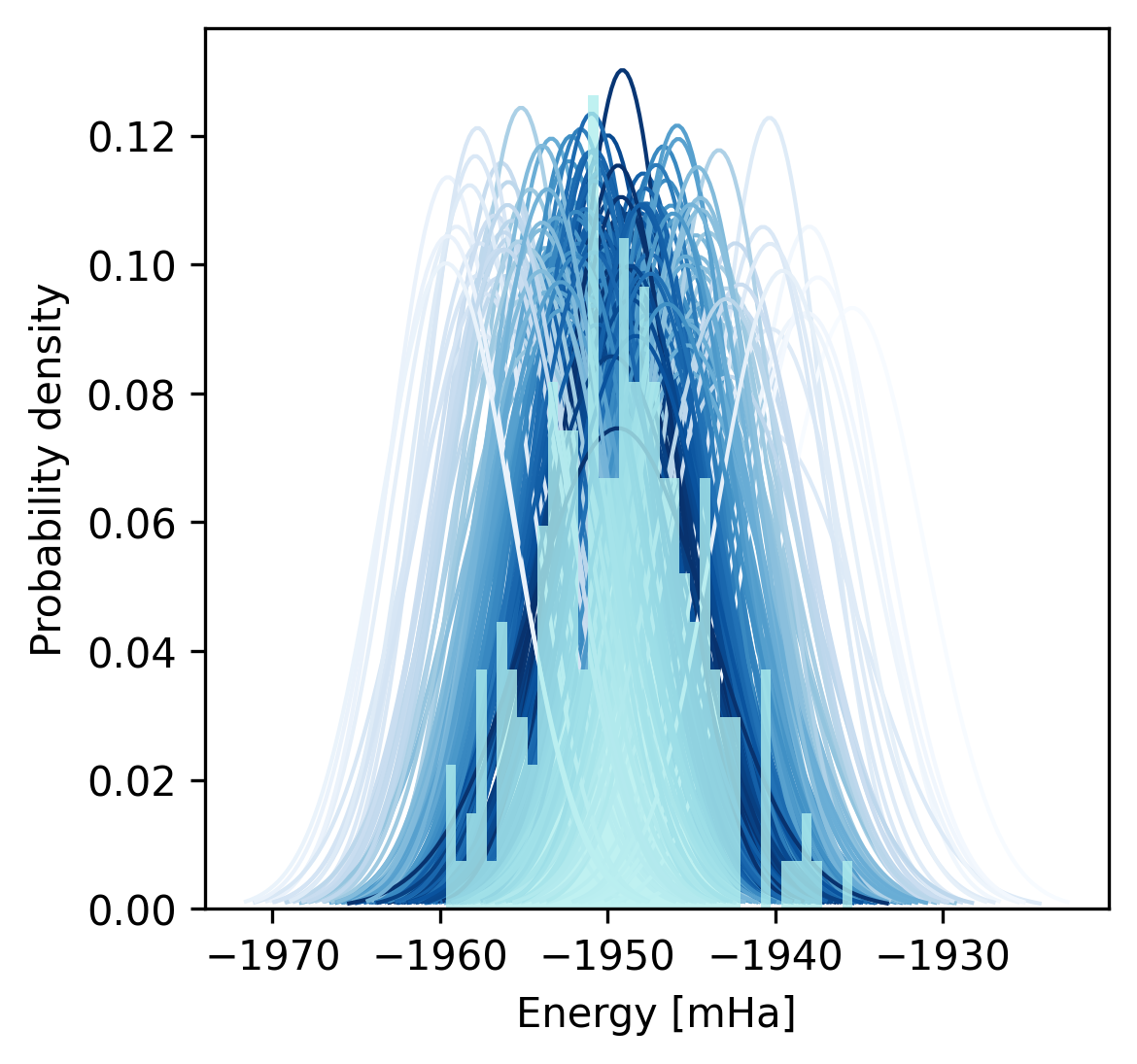
One might question whether bootstrapping is well-motivated here. A priori, one has no reason to expect acceptable agreement with the true population parameters, hence we ran 225 instances of our quantum experiment applied just to the diagonal terms of the Hamiltonian (given in Table 2), necessitating only computational basis measurements. We performed circuit shots in each experiment, for a combined total of point samples before assessing the quality of the bootstrapped distributions against the overall sample. The 225 quantum experiments provide a target standard deviation , indicated by the vertical line in Figure 15, and we compare with this the bootstrap standard deviations obtained per experiment.
In Figure 14 we plot the result of our bootstrapping test and see reasonable agreement with the true energy distribution obtained from the NISQ hardware; the standard deviations all coincide with the experimentally-obtained value to (on the order of chemical precision), as indicated in Figure 15, and therefore we employ bootstrapping with confidence.