Interactive Segmentation as Gaussian Process Classification
Abstract
Click-based interactive segmentation (IS) aims to extract the target objects under user interaction. For this task, most of the current deep learning (DL)-based methods mainly follow the general pipelines of semantic segmentation. Albeit achieving promising performance, they do not fully and explicitly utilize and propagate the click information, inevitably leading to unsatisfactory segmentation results, even at clicked points. Against this issue, in this paper, we propose to formulate the IS task as a Gaussian process (GP)-based pixel-wise binary classification model on each image. To solve this model, we utilize amortized variational inference to approximate the intractable GP posterior in a data-driven manner and then decouple the approximated GP posterior into double space forms for efficient sampling with linear complexity. Then, we correspondingly construct a GP classification framework, named GPCIS, which is integrated with the deep kernel learning mechanism for more flexibility. The main specificities of the proposed GPCIS lie in: 1) Under the explicit guidance of the derived GP posterior, the information contained in clicks can be finely propagated to the entire image and then boost the segmentation; 2) The accuracy of predictions at clicks has good theoretical support. These merits of GPCIS as well as its good generality and high efficiency are substantiated by comprehensive experiments on several benchmarks, as compared with representative methods both quantitatively and qualitatively. Codes will be released at https://github.com/zmhhmz/GPCIS_CVPR2023.
1 Introduction
Driven by the huge potential in reducing the pixel-wise annotation cost, interactive segmentation (IS) has sparked much research interest he2014interactive, which aims to segment the target objects under user interaction with less interaction cost. Among various types of user interaction xu2017deep; acuna2018efficient; castrejon2017annotating; ling2019fast; bai2014error; wu2014milcut; majumder2020two; zhang2020interactive, in this paper, we focus on the popular click-based mode, where positive annotations are clicked on the target object while negative ones are clicked in the background regions jang2019interactive; sofiiuk2020f; sofiiuk2021reviving; lin2022focuscut; chen2022focalclick.

Recent years have witnessed the promising success of deep learning (DL)-based methods in the IS task. The most commonly adopted research line is that the user interaction is encoded as click maps and fed into a deep neural network (DNN) together with input images to extract deep features for the subsequent segmentation xu2016deep; sofiiuk2021reviving. However, these methods generally suffer from two limitations: 1) As shown in Fig. 1 (a), after extracting the deep features, they generally perform pixel-wise classification without specific designs for the IS task. As a result, during the last-layer classification, the deep features of different pixels are not fully interactive and the information contained in clicked pixels cannot be finely propagated to other pixels under explicit regularization. 2) There is no explicit theoretical support that the clicked regions can be properly activated and correctly classified. Although some researchers have proposed different strategies, e.g., non-local-based modules chen2021conditional and the backpropagating refinement scheme jang2019interactive; sofiiuk2020f, they usually incur extra computational cost and are not capable enough to deal with the two problems simultaneously. Besides, the relations between deep features of different pixels are generally characterized and captured based on off-the-shelf network modules. Such implicit design makes it hard to clearly understand the working mechanism underlying these methods.
To alleviate these aforementioned issues, inspired by the intrinsic capabilities of Gaussian process (GP) models, e.g., explicitly measuring the relations between data points by a kernel function, and promoting accurate predictions at training data via interpolation, we rethink the IS task and attempt to construct a GP-based inference framework for the specific IS task. Concretely, as shown in Fig. 1 (b), we propose to treat the IS task from an alternative perspective and reformulate it as a pixel-level binary classification problem on each image, where clicks are viewed as training pixels with classification labels, i.e., foreground or background, and the unclicked points as the to-be-classified testing pixels. With such understanding, we construct the corresponding GP classification model. To solve it, we propose to utilize the amortized variational inference to efficiently approximate the intractable GP posterior in a data-driven manner, and then adopt the decoupling techniques wilson2020efficiently; wilson2021pathwise to achieve the GP posterior sampling with linear complexity. To improve the learning flexibility, we further embed the deep kernel learning strategy into the decoupled GP posterior inference procedure. Finally, by correspondingly integrating the derived GP posterior sampling mechanism with DNN backbones, we construct a GP Classification-based Interactive Segmentation framework, called GPCIS. In summary, our contributions are mainly three-fold:
1) We propose to carefully formulate the IS task as a Gaussian process classification model on each image. To adapt the GP model to the IS task, we propose specific designs and accomplish the approximation and efficient sampling of the GP posterior, which are then effectively integrated with the deep kernel learning mechanism for more flexibility.
2) We build a concise and clear interactive segmentation network under a theoretically sound framework. As shown in Fig. 1 (b), the correlation between the deep features of different pixels is modeled by GP posterior. With such explicit regularization, the information contained in clicks can be finely propagated to the entire image and boost the prediction of unclicked pixels. Besides, our method can provide rational theoretical support for accurate predictions at clicked points. These merits are finely validated in Sec. 5.2.
3) Extensive experimental comparisons as well as model verification comprehensively substantiate the superiority of our proposed GPCIS in segmentation quality and interaction efficiency. It is worth mentioning that the proposed GPCIS can consistently achieve superior performance under different backbone segmentors, showing its fine generality.
2 Related Work
In this section, we briefly review the related work on the click-based interactive segmentation (IS) task.
Traditional methods for IS grady2006random; gulshan2010geodesic; kim2010nonparametric; rother2004grabcut generally utilize the low-level features of to-be-segmented images and build optimization-based graphical models, which usually suffer from unsatisfactory performance and low efficiency. Motivated by the promising success of deep neural networks (DNN) long2015fully; chen2017deeplab in semantic segmentation, various methods have borrowed these pipelines for handling the IS task by transforming user interactions into click maps and taking them as the network input xu2016deep; liew2017regional; li2018interactive; lin2020interactive. In 99%AccuracyNet forte2020getting and RITM sofiiuk2021reviving, the mask predicted during the previous click was also regarded as the network input for helping the predictions for the current click. Recently, to better exploit the information contained in clicks and further propagate it to the entire image for promoting the segmentation of unclicked points, FCANet lin2020interactive put more emphasis on leveraging the first click and CDNet chen2021conditional designed the non-local-based conditional diffusion modules. Although these methods can deal with the relations between the features of different pixels to some extent, they can hardly provide any explicit theoretical basis for corrected predictions at clicked points. To this end, BRS jang2019interactive, f-BRS sofiiuk2020f, and CA kontogianni2020continuous have proposed to perform loss backpropagation during testing to adapt click maps or their network parameters to the current testing image. Clearly, the extra computation cost would adversely affect the efficiency of interactive segmentation. Recently, another research line, e.g., RIS-Net liew2017regional, FocalClick chen2022focalclick, and FocusCut lin2022focuscut, deals with the IS task from a local view to refine the segmentation results. Albeit attaining performance improvement, these methods have not fully exploited the relations between the deep features of clicks and those of unclicked points. Against this issue, in this paper, we build a concise and efficient model to explicitly model the relations between the deep features of the entire to-be-segmented image. It is worth noting that triebel2014active employs a Gaussian process model to develop an active learning framework for interactive segmentation, aiming to actively query pixels to be labeled.
3 Preliminaries: Gaussian Processes
Gaussian processes (GP) williams2006gaussian can be understood as the “Gaussian distribution over functions”. As a compelling tool, by directly modeling the prior and posterior of functions, it has been widely adopted in various tasks williams1995gaussian; nickisch2008approximations; liu2020gaussian. Mathematically, a GP is defined as a stochastic process where the joint distribution of any finite random variables is Gaussian. Define a mean function and a covariance function , a GP satisfies with mean and covariance matrix , for any finite observations . Specifically, for the GP prior, is generally assumed to be a constant zero function. The covariance function can be elaborately designed to model the correlations between the data points.
Given noise-free latent observations at training data , the GP posterior at testing data is written as williams2006gaussian:
| (1) |
where
| (2) |
As seen, the GP posterior utilizes the relations between the testing data and the training data to estimate the distribution of the function at , where the relations are explicitly measured by the kernel function .
4 Methodology
In this section, we firstly propose that the interactive segmentation (IS) problem can be regarded as a pixel-wise binary classification task on each input image. Based on such understanding, we carefully formulate this task with a GP classification model. Then, to solve it, we propose the corresponding algorithms to finely approximate and efficiently sample from GP posterior. Finally, by flexibly combining the GP model with DNN backbones, we construct the entire inference framework. The details are given below.
4.1 Model Formulation
For the interactive segmentation on an RGB image , users iteratively impose positive or negative clicks on the image to segment the target object, where is the number of the pixels; is the number of the interactive clicks; and is the label (i.e., foreground/background) of the click. By feeding the to-be-segmented image to a DNN , we can extract the feature representations as , where denotes the features of pixel . Given the features at clicked pixels and their labels , our goal is to predict the labels of the unclicked pixels with the features , where is the number of unclicked pixels. Next, we aim to solve the two core problems: ❶ How to finely model the relations between the deep features of different pixels and fully propagate the information contained in clicks for boosting the correct predictions at unclicked pixels? ❷ How to guide and promote accurate predictions at clicks?
Inspired by the appealing properties of Gaussian process (GP) models for our task, e.g., the capability of explicitly modeling the relations between data points and accurately interpolating the training data, we propose to rethink the IS task from a micro perspective and formulate it as a pixel-level binary classification task on each image, where the features of clicked pixels are regarded as training data with labels and those of unclicked pixels as testing data. Based on such understanding, we attempt to handle the pixel-wise binary classification task via GP models.
Specifically, we define a GP with a zero-mean prior and a covariance function over the classification function , which takes the feature of pixel as input and outputs the score for binary classification, i.e., positive score for foreground and negative score for background. Then the inference process from the available click information to the unknown labels at can be transformed into the following GP classification model which aims to solve the posterior distribution of the labels given , mathematically expressed as:
| (3) |
where is the GP posterior. For the binary classification task, it is conventionally set that , where is the sigmoid function nickisch2008approximations.
As seen, the integral in Eq. (3) is explicitly intractable for our task. Fortunately, if we can obtain the GP posterior, the integral can be approximated with a Monte Carlo method hensman2015scalable. Specifically, suppose is sampled from the derived GP posterior, we can approximately get that the probability of classifying the testing data into the foreground is . Hence, the key is how to obtain the GP posterior . Besides, after obtaining the GP posterior, how to achieve efficient sampling from it is also worth exploring since high inference efficiency is critical for the IS task. Next, we will answer the two questions.
4.2 GP Posterior Approximation and Sampling
In this subsection, we aim to approximate the GP posterior and achieve efficient sampling.
GP posterior approximation. It is easily known that the GP posterior can be rewritten as:
| (4) |
where follows a Gaussian distribution as defined in Eq. (1); ; and . For the classification task, due to the non-Gaussian likelihood , is non-Gaussian and leads to that the GP posterior in Eq. (4) is intractable. Against this issue, previous methods opper2009variational; nickisch2008approximations; hensman2015scalable have proposed to approximate with a Gaussian variational distribution by minimizing their KL divergence as:
| (5) |
To solve Eq. (5), conventional variational inference-based methods opper2009variational; nickisch2008approximations; hensman2015scalable independently optimize the objective on each training task (i.e., each training image in our IS case). These methods are generally time-consuming and fail to exploit the shared information among different images. In contrast, we imitate the amortized variation inference kingma2013auto to efficiently infer from and the distribution parameters for can be flexibly learned based on all the training images (i.e., the whole benchmark dataset) in an end-to-end manner. Specifically, the variational distribution is set as:
| (6) |
where the mean function is designed as:
| (7) |
where MLP represents a multi-layer perceptron parameterized by , which transforms the features from to . The activation function is the smooth version of ReLU, whose output is consistently positive. By empirically setting a small variance as 0.01, for any , we have , which has the same positive/negative sign as and helps the correct category prediction at clicks.
By substituting Eq. (6) and derived in Eq. (4), we can rewrite the KL divergence in Eq. (5) as: 11 1 Please refer to Supplementary Material (SM) for detailed derivations.
| (8) |
where we simplify as .
By optimizing Eq. (8) over all the training images in an end-to-end manner, we can obtain the variational distribution . Then by substituting it into Eq. (4), we can easily derive that the GP posterior is Gaussian and can be approximated as: 1
| (9) |
where
| (10) |

Decoupling GP posterior for efficient sampling. From the analysis of Eq. (3), by sampling from the tractable GP posterior in Eq. (9), we can obtain the classification probability for unclicked pixels as . To sample , the standard approach is to compute with wilson2020efficiently. As seen, the computation cost of is cubic w.r.t. the number of unclicked pixels , i.e., , which severely affects the efficiency. Against this issue, we propose to adopt the techniques wilson2020efficiently; wilson2021pathwise which decouple the GP posterior into a weight-space prior term and a function-space update term, largely reducing the sampling cost without sacrificing interpolation accuracy at clicks. Then, for the GP posterior in Eq. (9), we can derive the sampling framework as wilson2020efficiently; wilson2021pathwise: 1
| (11) |
where ; ; is constructed by a set of Fourier bases and the -th basis is expressed as rahimi2007random:
| (12) |
where ; ; ; is sampled from the spectral density of the kernel . We will carefully design the kernel function in Sec. 4.3.
In practice, considering and , the cost of sampling from Eq. (11) is reduced from to wilson2020efficiently; wilson2021pathwise. Note that in our practical implementation, to keep consistency with most DL-based methods sofiiuk2021reviving; chen2021conditional; chen2022focalclick, we execute an inference on the entire image with pixels. That is to say, we also sample using Eq. (11) in parallel with , by replacing the subscripts (i.e., the number of unclicked pixels) with the total number of pixels . Then, we can obtain the entire prediction results of pixels, i.e., .
Remark 1: It is worth mentioning that the proposed sampling strategy in Eq. (11) possesses two inherent characteristics: ❶ The relations between the deep features of clicked points and those of the unclicked points are fully utilized and explicitly modeled by the function-space update term, which enables the information contained in clicked regions to propagate to other regions. ❷ For training stability, the matrix inversion in Eqs. (8) (11) is practically computed by , where is empirically set to 0.01 during training. In Eq. (11), if we replace the number of the unclicked pixels (subscripts ) with the number of clicked pixels (subscripts ) and set a small enough , we can obtain that , showing that the sampled has the same positive/negative sign as the labels . This implies that the proposed sampling strategy can provide theoretical support for encouraging accurate predictions at clicked points. The two characteristics are validated by the model verification in Sec. 5.2.
4.3 Double Space Deep Kernel Learning
From Eqs. (11) and (12), we can see that the kernel affects both the function-space update and weight-space prior terms. Designing a proper and flexible kernel is important for better modeling the relations between pixels and extracting the prior knowledge underlying the segmentation function.
In the decoupling paradigm wilson2020efficiently; wilson2021pathwise, the adopted kernel function is generally pre-defined and fixed, which would lead to two potential limitations: 1) In function space, the kernel representation capacity would be constrained and the similarity measure between data points may not be optimal for our task; 2) In weight space, the prior term is not flexible enough to capture the prior knowledge underlying the IS task. Against these issues, instead of adopting the fixed manually-designed kernels, inspired by deep kernel learning (DKL) wilson2016deep, we propose to flexibly learn the kernel function in both function space and weight space from the abundant training images in a data-driven manner.
Specifically, we propose to perform double space DKL on , where represents the concatenation of the deep features and the image RGB values at pixel . Here, the concatenation of input image is for providing more information as validated in Sec. 5.4. In function space, to improve representation flexibility, we select a modified radial basis function (RBF) with scaling hyperparamters as the kernel function: where and is the -th element of . In weight space, since the hyperparameters are updating during network training, it is not suitable to sample in Eq. (12) from the kernel’s spectral density, thus it is set as a learnable parameter. To further improve flexibility and representation capacity of the weight-space prior term for better extracting the image prior, we parameterize the prior distribution of as . These hyperparameters in the double space, including , and , are trained in an end-to-end manner based on the entire training dataset.
Compared to the pre-fixed kernel design manner, the proposed double space DKL strategy is more flexible and it can utilize the powerful representation ability of DNNs to promote the performance, which is validated in Sec. 5.4.
4.4 The Proposed GPCIS Framework
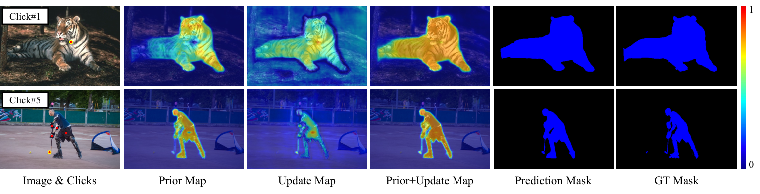
Based on the derived GP posterior sampling procedure as well as the double space DKL mechanism, we can correspondingly construct the entire framework, called Gaussian Process Classification-based Interactive Segmentation (GPCIS). As presented in Fig. 2, similar to sofiiuk2021reviving; chen2021conditional; chen2022focalclick, we firstly input the image and the click maps together with the previous mask to a general backbone segmentor for extracting the deep features . By feeding the concatenation of and the image , i.e., , to the efficient GP posterior sampling framework in Eq. (11), we can generate a weight-space prior map and a function-space update map. Finally, we can obtain the segmentation result by adding the two maps followed by a sigmoid function.
Remark 2: As seen, in our proposed GPCIS, the correlation modeling on the deep features of different pixels are explicitly corresponding to the derived GP posterior sampling strategy. Compared to the current methods jang2019interactive; sofiiuk2020f; chen2021conditional; lin2022focuscut; chen2022focalclick which are implicitly built based on off-the-shelf network modules, our method has a clearer working mechanism.
Network training. For the proposed GPCIS framework, the involved parameters are automatically learned from the training data in an end-to-end manner, including for the backbone segmentor, for variational distribution , for function-space DKL, and for weight-space DKL. The training loss is set as: 22 2 The entire algorithm flowchart is provided in SM.
| (13) |
where is the output segmentation result; is the ground truth mask; is the weighting parameter which is empirically set to ; is the normalized focal loss sofiiuk2019adaptis which is widely adopted by the existing IS methods sofiiuk2021reviving; chen2021conditional; chen2022focalclick; is the optimization objective in Eq. (8).
5 Experiments
5.1 Experimental Settings
Datasets. We conduct IS experiments on four widely-adopted datasets: 1) GrabCut rother2004grabcut contains 50 images with single object masks; 2) Berkeley mcguinness2010comparative contains 96 images with 100 object masks; 3) SBD hariharan2011semantic contains 20,172 masks for 8,498 images as the training set, 6,671 instance-level masks for 2,857 images as the validation set. The annotated masks are polygonal; 4) DAVIS perazzi2016benchmark contains 345 frames randomly sampled from 50 videos, with high-quality masks. We adopt the training split of SBD as the training set and take the other mentioned datasets for evaluation.
Evaluation metrics. Following xu2016deep; li2018interactive; sofiiuk2021reviving; lin2022focuscut; chen2022focalclick, we adopt the same strategy to simulate the clicks, which generates the next click at the center of the largest error region by comparing the prediction and ground truth. The Number of Clicks (NoC) is adopted as the metric, which counts the average number of clicks needed to achieve the target Intersection over Union (IoU). Following xu2016deep; li2018interactive; sofiiuk2021reviving; lin2022focuscut; chen2022focalclick, we set the IoU threshold to 85% and 90%. The evaluation metrics are denoted as NoC@85 and NoC@90, respectively. The default maximum number of clicks is 20. The Number of Failures (NoF) is also reported and it counts the number of images that cannot achieve the target IoU within the specified maximum number of clicks. Besides, we also report the average IoU at the N-th click, denoting IoU&N. To evaluate the correctness of predictions at clicks, we propose a new metric as NoIC which counts the Number of Incorrectly classified Clicks over a testing dataset. Lower NoC, NoF, and NoIC, as well as higher IoU&N, indicate better performance.
Implementation details. We implement the proposed framework with PyTorch paszke2019pytorch based on 4 NVIDIA V100 GPUs. For the backbone segmentor, we adopt three different networks, including SegFormerB0-S2 xie2021segformer; chen2022focalclick, HRNet18s-S2 wang2020deep; chen2022focalclick, and DeepLabv3+ chen2018encoder with ResNet50 he2016deep, to substantiate the generality of our method. The initial learning rate is for SegFormerB0-S2 and ResNet50, and for HRNet18s-S2. It is divided by 10 at [190, 220] epochs and the total number of epochs is 230, as in chen2022focalclick. We adopt the Adam optimizer kingma2014adam with the total batch size of 64 and the training patch size of . For inferring in Eq. (6), we adopt a one-hidden-layer MLP with 96 hidden units. More details are provided in SM.
| NoIC | 36 | 30 | 21 | 15 | 15 | 8 | 2 |
|---|
| Backbone | Method | GrabCut rother2004grabcut | Berkeley mcguinness2010comparative | SBD hariharan2011semantic | DAVIS perazzi2016benchmark | Average | |||||
|---|---|---|---|---|---|---|---|---|---|---|---|
| NoC@85 | NoC@90 | NoC@85 | NoC@90 | NoC@85 | NoC@90 | NoC@85 | NoC@90 | NoC@85 | NoC@90 | ||
| DeepLab-LargeFOV chen2017deeplab | ∗ RIS-Net liew2017regional (’17) | - | 5.00 | - | 6.03 | - | - | - | - | - | - |
| CAN YuKoltun2016 | LD li2018interactive (’18) | 3.20 | 4.79 | - | - | 7.41 | 10.78 | 5.95 | 9.57 | - | - |
| FCN long2015fully | ∗DOS xu2016deep (’16) | 5.08 | 6.08 | - | - | 9.22 | 12.80 | 9.03 | 12.58 | - | - |
| ∗CMG majumder2019content (’19) | - | 3.58 | - | 5.60 | - | - | - | - | - | - | |
| DenseNet huang2017densely | BRS jang2019interactive (’19) | 2.60 | 3.60 | - | 5.08 | 6.59 | 9.78 | 5.58 | 8.24 | - | 6.68 |
| Xception-65 chollet2017xception | ∗CA kontogianni2020continuous (’20) | - | 3.07 | - | 4.94 | - | - | 5.16 | - | - | - |
| SegFormerB0-S2 xie2021segformer; chen2022focalclick | RITM sofiiuk2021reviving (’21) | 1.62 | 1.82 | 1.84 | 2.92 | 4.26 | 6.38 | 4.65 | 6.13 | 3.09 | 4.31 |
| FocalClick chen2022focalclick (’22) | 1.66 | 1.90 | - | 3.14 | 4.34 | 6.51 | 5.02 | 7.06 | - | 4.65 | |
| GPCIS (Ours) | 1.60 | 1.76 | 1.84 | 2.70 | 4.16 | 6.28 | 4.45 | 6.04 | 3.01 | 4.20 | |
| HRNet18s-S2 wang2020deep; chen2022focalclick | RITM sofiiuk2021reviving (’21) | 2.00 | 2.24 | 2.13 | 3.19 | 4.29 | 6.36 | 4.89 | 6.54 | 3.33 | 4.58 |
| FocalClick chen2022focalclick (’22) | 1.86 | 2.06 | - | 3.14 | 4.30 | 6.52 | 4.92 | 6.48 | - | 4.55 | |
| GPCIS (Ours) | 1.74 | 1.94 | 1.83 | 2.65 | 4.28 | 6.25 | 4.62 | 6.16 | 3.12 | 4.25 | |
| ResNet50 he2016deep | ∗FCANetlin2020interactive (’20) | 2.18 | 2.62 | - | 4.66 | - | - | 5.54 | 8.83 | - | - |
| f-BRS-B sofiiuk2020f (’20) | 2.20 | 2.64 | 2.17 | 4.22 | 4.55 | 7.45 | 5.44 | 7.81 | 3.59 | 5.53 | |
| CDNet chen2021conditional (’21) | 2.22 | 2.64 | - | 3.69 | 4.37 | 7.87 | 5.17 | 6.66 | - | 5.22 | |
| RITM sofiiuk2021reviving (’21) | 2.16 | 2.30 | 1.90 | 2.95 | 3.97 | 5.92 | 4.56 | 6.05 | 3.15 | 4.31 | |
| FocusCut lin2022focuscut (’22) | 1.60 | 1.78 | 1.86 | 3.44 | 3.62 | 5.66 | 5.00 | 6.38 | 3.02 | 4.32 | |
| FocalClick chen2022focalclick (’22) | 1.92 | 2.14 | 1.87 | 2.86 | 3.84 | 5.82 | 4.61 | 6.01 | 3.06 | 4.21 | |
| GPCIS (Ours) | 1.64 | 1.82 | 1.60 | 2.60 | 3.80 | 5.71 | 4.37 | 5.89 | 2.85 | 4.00 | |
| Method | Berkeley mcguinness2010comparative | DAVIS perazzi2016benchmark | #Params (MB) | SPC (ms) | ||||||||
|---|---|---|---|---|---|---|---|---|---|---|---|---|
| NoC100@90 | NoF100@90 | IoU&1 | IoU&5 | NoIC | NoC100@90 | NoF100@90 | IoU&1 | IoU&5 | NoIC | |||
| f-BRS-B sofiiuk2020f | 6.21 | 2 | 77.06% | 85.00% | 1 | 22.62 | 57 | 70.97% | 83.87% | 0 | 39.44 | 116.53 |
| CDNet chen2021conditional | - | - | - | - | - | 18.59 | 48 | - | - | - | 39.90 | 57.76 |
| RITM sofiiuk2021reviving | 3.75 | 1 | 76.88% | 94.66% | 2 | 18.09 | 51 | 72.89% | 89.14% | 74 | 39.48 | 34.24 |
| FocusCut lin2022focuscut | 4.63 | 1 | 78.89% | 92.89% | 1 | 19.00 | 45 | 72.71% | 87.58% | 6 | 40.36 | 950.68 |
| FocalClick chen2022focalclick | 4.46 | 2 | 75.59% | 94.90% | 0 | 17.74 | 49 | 70.76% | 88.90% | 42 | 39.50 | 41.80 |
| GPCIS (Ours) | 3.36 | 1 | 79.43% | 95.11% | 0 | 17.03 | 44 | 75.67% | 89.60% | 2 | 39.39 | 38.82 |
5.2 Model Verification
Decoupled GP posterior. We firstly execute a model verification experiment to present the working mechanism underlying the decoupled GP posterior sampling framework Eq. (11). From Fig. 3, we can clearly observe that the probability maps output by the weight-space prior term can provide rough segmentation results of the target objects. This is mainly attributed to the proposed weight space DKL strategy which can flexibly learn the prior knowledge for the IS task from the training dataset. Besides, as presented, the function-space update term compensates the prior term by utilizing relations of pixels and assigning a larger probability to unclicked pixels semantically similar to the clicks. Then it helps achieve better predictions of unclicked points by propagating the information of the clicks, such as the regions far from the click on the tiger and the long stick. Attributed to the mutual promotion of the weight-space prior and function-space update, our method obtains accurate segmentation results, approaching the ground truth (GT) masks. The results finely comply with the analysis in Remark 1 ❶ and validate the rationality of our proposed method.
Accuracy at clicked points. Based on the backbone ResNet50 and the DAVIS dataset, we utilize the NoIC metric to evaluate the prediction accuracy at clicks of our proposed GPCIS under different during testing. From Table 1 where is set to 0.01 during training, we can easily observe that as gradually gets smaller during testing, NoIC almost shows a clear downward trend, which supports the claim in Remark 1 ❷ that our proposed GPCIS can achieve accurate predictions at clicks with small enough . Hence, in the following experiments, we reasonably adopt a larger as for training stability and a smaller as during testing for more accurate predictions at clicks.
5.3 Performance Evaluation
In this section, based on the four datasets, i.e., GrabCut, Berkeley, SBD, and DAVIS, we comprehensively validate the effectiveness of our proposed method by comparing it with a series of IS methods liew2017regional; li2018interactive; xu2016deep; majumder2019content; jang2019interactive; kontogianni2020continuous; chen2022focalclick; lin2020interactive; sofiiuk2020f; chen2021conditional; lin2022focuscut. For fair comparisons with the current state-of-the-art (SOTA) methods chen2022focalclick; lin2020interactive; sofiiuk2020f; chen2021conditional; lin2022focuscut, we separately implement our proposed GPCIS with the backbone segmentor SegFormerB0-S2 and HRNet18s-S2 adopted by chen2022focalclick, and with ResNet50 widely adopted by lin2020interactive; sofiiuk2020f; chen2021conditional; lin2022focuscut. Note that our proposed method is orthogonal to most of the competitors and yet we do not adopt their exclusive designs, such as cropping click-centered patches with adaptive scopes in FocusCut lin2022focuscut, and local refinement and progressive merge in FocalClick chen2022focalclick. RITM sofiiuk2021reviving is also reimplemented as our baseline under the same experimental settings. 33 3 More experimental results are provided in SM.


Quantitative evaluation. Table 2 lists the NoC@85 and NoC@90 of all the comparing methods on the four different datasets. We can clearly find that the proposed GPCIS consistently achieves the lowest average NoC@85 and NoC@90 under three different backbone segmentors, which substantiates its promising effectiveness and good generality. Note that although our method does not introduce the extra processing strategies contained in the SOTA method FocusCut, e.g., cropping click-centered patches with adaptive scopes, it can still obtain the superior (Berkeley & DAVIS) or at least comparable (GrabCut & SBD) performance to FocusCut.
For comprehensive comparisons, we provide more quantitative results on different metrics as well as the number of network parameters and inference efficiency. As listed in Table 3, the proposed GPCIS consistently outperforms other competing methods on NoC100@90, NoF100@90, IoU&1, IoU&5, and the model size, where NoC100@90 and NoF100@90 represent the numbers of clicks and failures to get 90% IoU within 100 clicks, respectively. For NoIC and SPC, it still performs competing and is comparable to the first rank. From Table 2 and Table 3, we can easily conclude that compared to other comparing methods, our proposed GPCIS shows better generality and it has the capability to efficiently attain higher segmentation accuracy with fewer clicks and fewer failure cases. This indicates that our method has good potential for practical IS. Note that compared to the baseline RITM, our inference speed is slightly slower due to the proposed GP posterior inference procedure. However, this cost is acceptable or even negligible considering the performance gains brought by our method.
Qualitative evaluation. Fig. 4 presents the visualization comparisons on the output probability maps of different methods. As seen, for RITM and FocalClick, the regions far from the click cannot be properly and fully activated and have low prediction probability. Although FocusCut confidently segments the main part of the object, it mistakenly leaves out the upper part with low prediction probability. Comparatively, our proposed GPCIS achieves better segmentation results and approaches the GT mask, which is mainly attributed to the explicit modeling of the semantic relations between pixels. To fully substantiate the effectiveness of our proposed inference process, we also provide more visual comparisons with the baseline RITM. From the first row in Fig. 5, we can observe that without fully utilizing the information contained in clicks, RITM fails to finely segment the whole target object. In contrast, our method almost accomplishes the accurate segmentation of the three target instances, i.e., two persons and a drum, within three clicks. Besides, the second row shows that from the 3 to the 16 clicks, RITM repetitively clicks in the same location because it cannot provide correct predictions at clicks. However, with good theoretical support, GPCIS alleviates this issue and obtains a 97% IoU within 8 clicks.
5.4 Ablation Studies
Based on the backbone segmentor ResNet50, we execute an ablation study to quantitatively evaluate the effect of the modules involved in our method on the average NoC@85/90 over GrabCut, Berkeley, SBD and DAVIS. Table 4 reports the results under different settings where variant (e) is the final strategy we adopt in comparison experiments above. By comparing (a) and (e), we can easily find that the proper guidance of is indeed helpful for network learning. In (b), we discard the deep kernel learning mechanism in function space and fix the kernel hyperparameters as and (). Similarly, in (c), we discard the deep kernel learning mechanism in weight space and set , , , and . During network training, they are not updated. As expected, without the DKL design in double space, the network flexibility is weakened, leading to degraded performance. Besides, by comparing (d) and (e), it shows that the concatenation of input image with deep features shown in Fig. 2 can further boost the information propagation across pixels and bring better segmentation performance.
| Variants | DKL-F | DKL-W | Concat | Avg. NoC@85 | Avg. NoC@90 | |
|---|---|---|---|---|---|---|
| (a) | ✗ | ✓ | ✓ | ✓ | 2.98 | 4.07 |
| (b) | ✓ | ✗ | ✓ | ✓ | 3.00 | 4.16 |
| (c) | ✓ | ✓ | ✗ | ✓ | 3.10 | 4.34 |
| (d) | ✓ | ✓ | ✓ | ✗ | 2.96 | 4.10 |
| (e) | ✓ | ✓ | ✓ | ✓ | 2.85 | 4.00 |
6 Conclusion
In this paper, for the interactive segmentation task, we have dived into a new perspective and regarded it as a pixel-wise binary classification problem on each input image. Based on such understanding, we have formulated the task as a Gaussian process classification model. To solve this model, we have proposed to variationally approximate the GP posterior in a data-driven manner, along with a decoupled sampling strategy with linear complexity. Correspondingly, we have constructed an efficient and flexible GP classification framework integrated with double space deep kernel learning, called GPCIS, which has clear working mechanism. Based on several benchmark datasets and different backbone segmentors, we have conducted comprehensive experiments as well as model verification, which fully substantiated the superiority of our proposed GPCIS as well as its rational theoretical support for correct predictions at clicks. With high efficiency and fine generality, the proposed GPCIS should be a potential driver for the interactive segmentation field.
References
- (1) David Acuna, Huan Ling, Amlan Kar, and Sanja Fidler. Efficient interactive annotation of segmentation datasets with Polygon-RNN++. In Proceedings of the IEEE/CVF International Conference on Computer Vision, pages 859–868, 2018.
- (2) Junjie Bai and Xiaodong Wu. Error-tolerant scribbles based interactive image segmentation. In Proceedings of the IEEE/CVF International Conference on Computer Vision, pages 392–399, 2014.
- (3) Lluis Castrejon, Kaustav Kundu, Raquel Urtasun, and Sanja Fidler. Annotating object instances with a Polygon-RNN. In Proceedings of the IEEE/CVF International Conference on Computer Vision, pages 5230–5238, 2017.
- (4) Liang-Chieh Chen, George Papandreou, Iasonas Kokkinos, Kevin Murphy, and Alan L Yuille. Deeplab: Semantic image segmentation with deep convolutional nets, atrous convolution, and fully connected CRFS. IEEE Transactions on Pattern Analysis and Machine Intelligence, 40(4):834–848, 2017.
- (5) Liang-Chieh Chen, Yukun Zhu, George Papandreou, Florian Schroff, and Hartwig Adam. Encoder-decoder with atrous separable convolution for semantic image segmentation. In Proceedings of the European Conference on Computer Vision, pages 801–818, 2018.
- (6) Xi Chen, Zhiyan Zhao, Feiwu Yu, Yilei Zhang, and Manni Duan. Conditional diffusion for interactive segmentation. In Proceedings of the IEEE/CVF International Conference on Computer Vision, pages 7345–7354, 2021.
- (7) Xi Chen, Zhiyan Zhao, Yilei Zhang, Manni Duan, Donglian Qi, and Hengshuang Zhao. FocalClick: Towards practical interactive image segmentation. In Proceedings of the IEEE/CVF International Conference on Computer Vision, pages 1300–1309, 2022.
- (8) François Chollet. Xception: Deep learning with depthwise separable convolutions. In Proceedings of the IEEE/CVF International Conference on Computer Vision, pages 1251–1258, 2017.
- (9) Mark Everingham, Luc Van Gool, Christopher KI Williams, John Winn, and Andrew Zisserman. The PASCAL visual object classes (VOC) challenge. International Journal of Computer Vision, 88(2):303–338, 2010.
- (10) Marco Forte, Brian Price, Scott Cohen, Ning Xu, and François Pitié. Getting to 99% accuracy in interactive segmentation. arXiv preprint arXiv:2003.07932, 2020.
- (11) Leo Grady. Random walks for image segmentation. IEEE Transactions on Pattern Analysis and Machine Intelligence, 28(11):1768–1783, 2006.
- (12) Varun Gulshan, Carsten Rother, Antonio Criminisi, Andrew Blake, and Andrew Zisserman. Geodesic star convexity for interactive image segmentation. In IEEE Computer Society Conference on Computer Vision and Pattern Recognition, pages 3129–3136, 2010.
- (13) Bharath Hariharan, Pablo Arbeláez, Lubomir Bourdev, Subhransu Maji, and Jitendra Malik. Semantic contours from inverse detectors. In Proceedings of IEEE International Conference on Computer Vision, pages 991–998, 2011.
- (14) Jia He, Chang-Su Kim, and C-C Jay Kuo. Interactive segmentation techniques: Algorithms and performance evaluation. Springer, 2014.
- (15) Kaiming He, Xiangyu Zhang, Shaoqing Ren, and Jian Sun. Deep residual learning for image recognition. In Proceedings of the IEEE/CVF International Conference on Computer Vision, pages 770–778, 2016.
- (16) James Hensman, Alexander Matthews, and Zoubin Ghahramani. Scalable variational gaussian process classification. In Artificial Intelligence and Statistics, pages 351–360. PMLR, 2015.
- (17) Gao Huang, Zhuang Liu, Laurens Van Der Maaten, and Kilian Q Weinberger. Densely connected convolutional networks. In Proceedings of the IEEE/CVF International Conference on Computer Vision, pages 4700–4708, 2017.
- (18) Won-Dong Jang and Chang-Su Kim. Interactive image segmentation via backpropagating refinement scheme. In Proceedings of the IEEE/CVF International Conference on Computer Vision, pages 5297–5306, 2019.
- (19) Tae Hoon Kim, Kyoung Mu Lee, and Sang Uk Lee. Nonparametric higher-order learning for interactive segmentation. In IEEE Computer Society Conference on Computer Vision and Pattern Recognition, pages 3201–3208, 2010.
- (20) Diederik P Kingma and Jimmy Ba. Adam: A method for stochastic optimization. arXiv preprint arXiv:1412.6980, 2014.
- (21) Diederik P Kingma and Max Welling. Auto-encoding variational Bayes. arXiv preprint arXiv:1312.6114, 2013.
- (22) Theodora Kontogianni, Michael Gygli, Jasper Uijlings, and Vittorio Ferrari. Continuous adaptation for interactive object segmentation by learning from corrections. In Proceedings of the European Conference on Computer Vision, pages 579–596, 2020.
- (23) Zhuwen Li, Qifeng Chen, and Vladlen Koltun. Interactive image segmentation with latent diversity. In Proceedings of the IEEE/CVF International Conference on Computer Vision, pages 577–585, 2018.
- (24) JunHao Liew, Yunchao Wei, Wei Xiong, Sim-Heng Ong, and Jiashi Feng. Regional interactive image segmentation networks. In Proceedings of IEEE International Conference on Computer Vision, pages 2746–2754, 2017.
- (25) Zheng Lin, Zheng-Peng Duan, Zhao Zhang, Chun-Le Guo, and Ming-Ming Cheng. FocusCut: Diving into a focus view in interactive segmentation. In Proceedings of the IEEE/CVF International Conference on Computer Vision, pages 2637–2646, 2022.
- (26) Zheng Lin, Zhao Zhang, Lin-Zhuo Chen, Ming-Ming Cheng, and Shao-Ping Lu. Interactive image segmentation with first click attention. In Proceedings of the IEEE/CVF International Conference on Computer Vision, pages 13339–13348, 2020.
- (27) Huan Ling, Jun Gao, Amlan Kar, Wenzheng Chen, and Sanja Fidler. Fast interactive object annotation with Curve-GCN. In Proceedings of the IEEE/CVF Conference on Computer Vision and Pattern Recognition, pages 5257–5266, 2019.
- (28) Haitao Liu, Yew-Soon Ong, Xiaobo Shen, and Jianfei Cai. When Gaussian process meets big data: A review of scalable gps. IEEE Transactions on Neural Networks and Learning Systems, 31(11):4405–4423, 2020.
- (29) Jonathan Long, Evan Shelhamer, and Trevor Darrell. Fully convolutional networks for semantic segmentation. In Proceedings of the IEEE/CVF International Conference on Computer Vision, pages 3431–3440, 2015.
- (30) Soumajit Majumder, Abhinav Rai, Ansh Khurana, and Angela Yao. Two-in-one refinement for interactive segmentation. In British Machine Vision Conference, 2020.
- (31) Soumajit Majumder and Angela Yao. Content-aware multi-level guidance for interactive instance segmentation. In Proceedings of the IEEE/CVF International Conference on Computer Vision, pages 11602–11611, 2019.
- (32) Kevin McGuinness and Noel E O’connor. A comparative evaluation of interactive segmentation algorithms. Pattern Recognition, 43(2):434–444, 2010.
- (33) Hannes Nickisch and Carl Edward Rasmussen. Approximations for binary Gaussian process classification. Journal of Machine Learning Research, 9(Oct):2035–2078, 2008.
- (34) Manfred Opper and Cédric Archambeau. The variational Gaussian approximation revisited. Neural Computation, 21(3):786–792, 2009.
- (35) Adam Paszke, Sam Gross, Francisco Massa, Adam Lerer, James Bradbury, Gregory Chanan, Trevor Killeen, Zeming Lin, Natalia Gimelshein, Luca Antiga, et al. PyTorch: An imperative style, high-performance deep learning library. Advances in Neural Information Processing Systems, 32, 2019.
- (36) Federico Perazzi, Jordi Pont-Tuset, Brian McWilliams, Luc Van Gool, Markus Gross, and Alexander Sorkine-Hornung. A benchmark dataset and evaluation methodology for video object segmentation. In Proceedings of the IEEE/CVF International Conference on Computer Vision, pages 724–732, 2016.
- (37) Ali Rahimi and Benjamin Recht. Random features for large-scale kernel machines. Advances in Neural Information Processing Systems, 20, 2007.
- (38) Carsten Rother, Vladimir Kolmogorov, and Andrew Blake. GrabCut: Interactive foreground extraction using iterated graph cuts. ACM Transactions on Graphics, 23(3):309–314, 2004.
- (39) Konstantin Sofiiuk, Olga Barinova, and Anton Konushin. AdaptIS: Adaptive instance selection network. In Proceedings of the IEEE/CVF International Conference on Computer Vision, pages 7355–7363, 2019.
- (40) Konstantin Sofiiuk, Ilia Petrov, Olga Barinova, and Anton Konushin. f-BRS: Rethinking backpropagating refinement for interactive segmentation. In Proceedings of the IEEE/CVF International Conference on Computer Vision, pages 8623–8632, 2020.
- (41) Konstantin Sofiiuk, Ilia A Petrov, and Anton Konushin. Reviving iterative training with mask guidance for interactive segmentation. arXiv preprint arXiv:2102.06583, 2021.
- (42) Rudolph Triebel, Jan Stühmer, Mohamed Souiai, and Daniel Cremers. Active online learning for interactive segmentation using sparse gaussian processes. In German Conference on Pattern Recognition, pages 641–652, 2014.
- (43) Jingdong Wang, Ke Sun, Tianheng Cheng, Borui Jiang, Chaorui Deng, Yang Zhao, Dong Liu, Yadong Mu, Mingkui Tan, Xinggang Wang, et al. Deep high-resolution representation learning for visual recognition. IEEE Transactions on Pattern Analysis and Machine Intelligence, 43(10):3349–3364, 2020.
- (44) Christopher Williams and Carl Rasmussen. Gaussian processes for regression. Advances in Neural Information Processing Systems, 8, 1995.
- (45) Christopher KI Williams and Carl Edward Rasmussen. Gaussian processes for machine learning, volume 2. MIT Press Cambridge, MA, 2006.
- (46) Andrew Gordon Wilson, Zhiting Hu, Ruslan Salakhutdinov, and Eric P Xing. Deep kernel learning. In Artificial Intelligence and Statistics, pages 370–378. PMLR, 2016.
- (47) James Wilson, Viacheslav Borovitskiy, Alexander Terenin, Peter Mostowsky, and Marc Deisenroth. Efficiently sampling functions from Gaussian process posteriors. In International Conference on Machine Learning, pages 10292–10302. PMLR, 2020.
- (48) James T Wilson, Viacheslav Borovitskiy, Alexander Terenin, Peter Mostowsky, and Marc Peter Deisenroth. Pathwise conditioning of Gaussian processes. Journal of Machine Learning Research, 22:105–1, 2021.
- (49) Jiajun Wu, Yibiao Zhao, Jun-Yan Zhu, Siwei Luo, and Zhuowen Tu. MILCut: A sweeping line multiple instance learning paradigm for interactive image segmentation. In Proceedings of the IEEE/CVF International Conference on Computer Vision, pages 256–263, 2014.
- (50) Enze Xie, Wenhai Wang, Zhiding Yu, Anima Anandkumar, Jose M Alvarez, and Ping Luo. SegFormer: Simple and efficient design for semantic segmentation with transformers. Advances in Neural Information Processing Systems, 34:12077–12090, 2021.
- (51) Ning Xu, Brian Price, Scott Cohen, Jimei Yang, and Thomas Huang. Deep interactive object selection. In Proceedings of the IEEE/CVF International Conference on Computer Vision, pages 373–381, 2016.
- (52) Ning Xu, Brian Price, Scott Cohen, Jimei Yang, and Thomas Huang. Deep GrabCut for object selection. In British Machine Vision Conference, 2017.
- (53) Fisher Yu and Vladlen Koltun. Multi-scale context aggregation by dilated convolutions. In International Conference on Learning Representations, 2016.
- (54) Shiyin Zhang, Jun Hao Liew, Yunchao Wei, Shikui Wei, and Yao Zhao. Interactive object segmentation with inside-outside guidance. In Proceedings of the IEEE/CVF International Conference on Computer Vision, pages 12234–12244, 2020.