DrMaMP: Distributed Real-time Multi-agent Mission Planning in Cluttered Environment
Abstract
Solving a collision-aware multi-agent mission planning (task allocation and path finding) problem is challenging due to the requirement of real-time computational performance, scalability, and capability of handling static/dynamic obstacles and tasks in a cluttered environment. This paper proposes a distributed real-time (on the order of millisecond) algorithm DrMaMP, which partitions the entire unassigned task set into subsets via approximation and decomposes the original problem into several single-agent mission planning problems. This paper presents experiments with dynamic obstacles and tasks and conducts optimality and scalability comparisons with an existing method, where DrMaMP outperforms the existing method in both indices. Finally, this paper analyzes the computational burden of DrMaMP which is consistent with the observations from comparisons, and presents the optimality gap in small-size problems.
I Introduction
Autonomous unmanned aerial vehicles (UAV) and unmanned ground vehicles (UGV) can replace humans for dangerous tasks such as surveillance and search-and-rescue. Recently, some receding-horizon motion planning methods [1, 2, 3] guide an autonomous robot to explore and go to a destination in a complex environment. These methods require a planning hierarchy. On top of this hierarchy, a path planner such as [4, 5] generates a sequence of sparse way-points based on the perception of the environment. Then a motion planner returns collision-free and dynamically feasible trajectories based on the sparse way-points. And the robot executes these trajectories and reaches the goal without any collisions. A group of autonomous robotic agents has more capabilities than a single robot in applications such as surveillance, information sensing, navigation, and search-and-rescue. If one can generate collision-free, non-conflict sparse paths for multiple agents and tasks at run-time, the robot swarm can explore a complex environment and execute complicated missions efficiently.

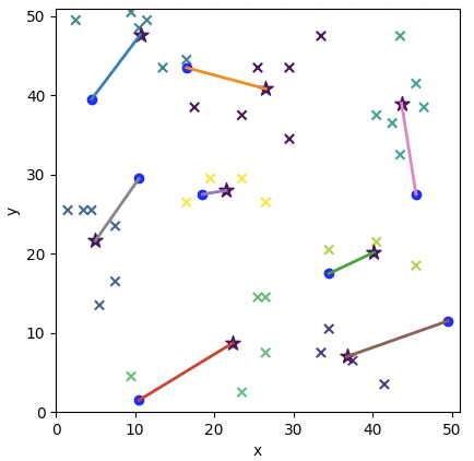
In this paper, a task is defined as a location of interest that one agent must visit. Given a set of agents and tasks, a collision-aware multi-agent mission planning (MAMP) problem is defined twofold, i.e. finding optimal and conflict-free task allocations for agents and then generating collision-free paths such that agents can visit these task positions. The former is categorized as a multi-agent task allocation (MATA) problem, and the latter is defined as a multi-agent path-finding (MAPF) problem. The optimal objective of MAPF is typically to minimize the total traveling distance. For a multi-agent system (MAS), real-time mission planning in a cluttered environment is necessary when deploying autonomous robots in a complex environment, especially when obstacles and tasks are dynamic. An example of MAMP problems is shown in Fig. 2(a). This paper only considers MAMP problems defined as ST-SR-TA (Single-Task Robots, Single-Robot Tasks, Time-Extended Assignment) problems [6]. Here, tasks are assumed to be homogeneous and independent of each other, i.e. no temporal logic requirements; agents are assumed to be homogeneous regarding mission functionality. Since this problem is proven to be NP-hard [6], there is a trade-off for MAMP problems between real-time performance and optimality. Furthermore, the scalability of an underlying algorithm, in terms of the number of agents and tasks, is crucial in MAS applications.
I-A Related Work
The literature on MAMP problems basically can be divided into two categories, i.e. solving MATA and MAPF problems sequentially or in an integrated way.
The methods related to MATA can be mainly categorized as auction-based and searching-based methods. Auction-based approaches are derived from a concept in finance where each agent aims to maximize their own reward by giving higher bids. And the process must consider maximizing a global reward and include conflict resolution. [7] utilizes auction-based protocols to bid task assignments. CBBA (Consensus-Based Bundle Algorithm)[8] employs a decentralized consensus procedure for task conflict resolution and then generates task allocation for agents. IACA (Iterated Auction Consensus Algorithm) [9] proposes a similar iterative but resilient auction process and can remove malicious bids during the auction. [10] proposed an auction-based algorithm to deal with task allocation problems with time window constraints. [11] produces task sequences with minimum communications by combining the greedy algorithm and the auction process. Although the auction-based approaches are decentralized, the process of auction and conflict resolution can be time-consuming, especially when the problem size is large. In addition, the auction heuristic barely includes environmental information, e.g. the impact of obstacles on the cost/reward. Thus, the auction result is not necessarily optimal when the obstacles are present and may even lead to a bad solution.
Search-based methods rely on a fixed structure of information, e.g. the number of assigned tasks for each agent is known and fixed. [12] proposes a decentralized genetic algorithm (GA) to search a task sequence parallelly. [13] proposes a graph-based search method to allocate tasks to agents given a finite linear temporal logic objective, where the allocation order is partially known. [14] builds an Optimized Directed Roadmap Graph (ODRM) by sampling first, and then navigates agents on this graph. Although searching paths on an ODRM is faster than on the most common occupancy grid map, generating and updating such a graph at run-time can be time-consuming in a cluttered and dynamic environment.
Due to the page limit, this paper omits the literature on MAPF problems because most of the recent literature focuses on the integration of MATA and MAPF problems. As for the literature on solving MATA and MAPF problems sequentially, they are mainly categorized as auction-based and search-based methods. Based on CBBA, [15] first generates task sequences without any obstacle information and then utilizes Dijkstra’s algorithm [4] to find collision-free paths given the sequences. [16] proposes a two-stage GA-based approach where each agent first determines its own task sequence using a genetic algorithm and then negotiates with other agents to exchange tasks if that reduces the cost. Then collision-free paths are generated similarly as [15].
There are also some special cases of MAMP problems that have risen significant interest, such as multi-agent pickup and delivery[17], and vehicle routing problems. Some special specifications are adopted for these problems. For example, the task set for each agent is prescribed; each agent can only be assigned one task; the initial positions for agents are the same, etc. This paper considers a general MAMP problem without these special specifications.
There is some literature on the integrated MAMP methods. [18] focuses on simultaneous task allocation and planning for a complex goal that consists of temporal logic sub-tasks. [18] emphasizes the capability of a heterogeneous robot team to perform a complex goal, whereas the MAMP problem in this paper focuses on homogeneous agents and tasks. [19], as a fully centralized optimization-based method, first obtains a single tour that connects all the tasks without any obstacle information by solving a traveling salesman problem; then uses a heuristic policy to partition the tour to generate a task allocation sequence for each agent; finally generates collision-free paths. Although [19] deals with the same problem with this paper, its computation time is stably around 55 seconds, with 5 - 20 agents and 10 - 50 tasks in a map with random obstacles.
From the methodology perspective, there are primarily three types of methods for MAMP problems with homogeneous agents/tasks and no temporal logic constraints, i.e. decentralized auction-based, distributed GA-based (genetic algorithm), and centralized optimization-based methods. Decentralized auction-based methods, as mentioned above, suffer from inefficient auction and negotiation processes and a lack of obstacle information during the auction process. Distributed GA-based methods might have good real-time performance for small-size problems but it notably depends on the selection of GA parameters. Also, many methods assume the number of assigned tasks for each agent is known and fixed, whereas this paper does not. As for optimization-based methods, they barely utilize obstacle information in the first place and are not in a distributed manner, i.e directly solving the entire allocation problem.
I-B Contributions and Notations
This paper proposes a real-time MAMP algorithm DrMaMP for homogeneous agents and tasks. DrMaMP first utilizes obstacle information as heuristics to approximate the cost of an ordered task allocation and path sequence by a metric from an unordered set. With this approximation, DrMaMP can partition the entire problem into several sub-problems and distribute them to each agent. Then each agent finds optimal task allocation and path sequence for each sub-problem. Due to the approximation and the distributed manner, DrMaMP makes a balance between computational performance and scalability. The main contributions are:
- 1.
a distributed real-time (on the order of millisecond) MAMP algorithm DrMaMP;
- 2.
capability of handling dynamic obstacles and tasks in a cluttered environment at run-time;
- 3.
good scalability in terms of the number of agents and tasks and relatively good optimality;
- 4.
computational burden analysis for DrMaMP.
Notations. Vectors, variables, and functions in multiple dimensions are in bold lowercase; matrices and sets are in uppercase. For a point , denotes a set containing that point as its only element. Set subtraction is . denotes the integer set. denotes the positive integer set. The cardinality of a set is denoted as .
II Problem Formulation
The configuration space, , is all positions in space reachable by an agent. Denote an agent positions set of agents, and is the position of agent . Denote a task positions set of tasks, and is the position of task . Define the agent and tasks index sets and , respectively. Suppose that an agent completes a task when the distance between two entities is less than a prescribed non-negative constant , i.e. . Denote an obstacle positions set as of obstacles, where is the position of obstacle . Denote as an ordered sequence of positions associated with agent which denotes a path starting from and ending at , where denotes the number of positions in .
Derived from [8], the collision-aware MATA problem is written as the following integer programming:
| (1a) | ||||||||
| (1b) | ||||||||
| (1c) | ||||||||
| (1d) | ||||||||
| (1e) | ||||||||
where if task is assigned to agent and otherwise; is the task assignment vector for agent , is the -th element of , and . The vector denotes an ordered sequence of tasks, i.e., the task allocation order, for agent ; its -th element is if task is the -th task of agent ’s assignment; if agent has no assignment. The collision-aware cost of task being assigned to agent followed by an order is defined by . In the context of mission planning, this cost typically represents traveling distance, fuel consumption, etc. Constraint (1b) indicates that each agent can be at most assigned with tasks; (1c) requires that each task must be assigned to only one agent; (1d) enforces that every task must be assigned.
Denote a task allocation order set . Given an order set and the current positions of agents , the collision-aware MAPF problem is written as:
| (2) | ||||||
where is the traveling distance of path . This paper assumes that if and only if .
Based on (1) and (2), the collision-aware MAMP problem in this paper is formulated as:
| (3) | ||||||
where evaluates agent ’s collision-aware traveling distance given a particular assignment and allocation order.
Solving the task assignment , the allocation order , and the collision-free path altogether is challenging because , , and are coupled together in (1), (2), and (3). Furthermore, the collision-aware MAMP problem (3) is not even tractable since it is proven to be NP-hard [6]. This paper attempts to obtain a sub-optimal solution to the collision-aware MAMP problem scalably and in real-time, especially when the environment is unconstructed and cluttered and the obstacles and tasks are potentially dynamic.
III Algorithm
This paper proposes a Distributed Real-time Multi-agent Mission Planning (DrMaMP) algorithm to obtain a sub-optimal solution to (3) in a scalable way. Instead of considering the exact coupled cost , DrMaMP utilizes task-based heuristics to approximate the cost of an ordered path by an unordered set. With this approximation, DrMaMP can partition the entire task set into several subsets and assign each task subset to one agent given the unordered heuristics. Then each agent only needs to solve a sub-problem, i.e. single-agent mission planning problem. Specifically, DrMaMP consists of three phases:
- 1.
Task Segmentation: partitioning the entire task set into several subsets;
- 2.
Cluster Assignment: assigning each agent a task subset;
- 3.
Single-Agent Mission Planning: finding an optimal task allocation order and collision-free path for each agent.
In Phase 1, given an objective defined in Section III-A, the entire task set is partitioned into subsets. In Phase 2, given an objective defined in Section III-B, each agent is assigned one task subset by solving an assignment problem. In Phase 3, after each agent is assigned with a task subset, it needs to solve a single-agent mission planning problem individually to find the optimal task allocation order and collision-free path. The computation can be distributed to each agent. A detailed explanation of the 3 phases is shown in the following subsections.


III-A Task Segmentation
The entire task set is partitioned into clusters , where each cluster includes possibly many tasks. Note that has not been assigned to any agents yet. The tasks within a cluster have a minimal distance to the centroid of this cluster. Such a task segmentation can be obtained by an iterative k-means clustering algorithm [20], which minimizes the summation of the within-cluster sum of squares (WCSS), i.e.
| (4) | ||||
where and is the task index set that is associated with the tasks within cluster ; is the centroid of tasks within . Denote .
As described in (3), the objective is to minimize the total traveling distance. But the cost of each agent visiting a known task set is unknown before a task allocation order is determined. Hence, for each task subset , an ordered sequence’s length is approximated by an unordered set’s WCSS, i.e. , since the tasks within have a less WCSS associated with than . The task segmentation problem (4) can be solved iteratively and the details are in Algorithm 1. An example is shown in Fig. 2(b).
III-B Cluster Assignment
Since an ordered sequence’s length is approximated by an unordered set’s WCSS in Algorithm 1, the cost of agent visiting a task subset is approximated by the distance between the agent and task subset’s centroid plus the subset’s WCSS, which is independent on the task allocation order. Then the task subset (cluster) assignment problem is written as an integer linear programming (5), where if agent is assigned with cluster and otherwise; defines the cost of cluster being assigned to agent , where the first term evaluates how far agent is to cluster and the second term estimates the cost of agent visiting all the tasks within cluster .
| (5a) | ||||||||
| (5b) | ||||||||
| (5c) | ||||||||
| (5d) | ||||||||
| (5e) | ||||||||
Constraint (5b) ensures that each cluster must be assigned with one agent; (5c) guarantees that each agent can be at most assigned to one cluster; (5d) enforces no unassigned cluster left. Constraint (5c) considers a situation when the number of agents is greater than the number of nonempty clusters. This situation can happen at run-time when some tasks are completed. The cluster assignment problem (5) can be solved by some constrained integer linear programming solvers such as OR-Tools [21].
III-C Single-Agent Mission Planning
After each agent is assigned a task cluster, the task allocation orders and the collision-free paths need to be determined. This problem can be distributed to agents parallelly, and agent solves its own sub-problem by formulating it as a Travelling Salesperson Problem (TSP), where the nodes are the agent itself and its assigned tasks. A path-finding algorithm generates collision-free paths for every pair of nodes and the length of these paths is the traveling cost from one node to another. This paper utilizes Lazy Theta* [5] as the path-finding algorithm due to fewer line-of-sight checks. The single-agent mission planning problem can be written as an integer linear program (6a) with Miller–Tucker–Zemlin (MTZ) formulation [23],
| (6a) | ||||||||
| (6b) | ||||||||
| (6c) | ||||||||
| (6d) | ||||||||
| (6e) | ||||||||
| (6f) | ||||||||
| (6g) | ||||||||
| (6h) | ||||||||
where denotes the number of nodes; node 1 always indicates the agent’s current position; if the agent goes from node to node , ; is a dummy variable to indicate tour ordering such that implies node is visited before node ; is the cost of agent traveling from node to node , which is the length of the underlying collision-free path.
The constraints (6c) - (6e) guarantees only one tour covering all nodes [23]. The constraints (6f) - (6g) guarantees that each node is visited from another node, and from each node, there is a departure to another node. The constraint (6h) indicates that the agent does not go back to its initial position after visiting all the tasks. One can change (6h) if the agent needs to go back to a base. To ensure that there is no collision between agents, each agent considers the other agents as obstacles. Details are shown in Algorithm 3. An example is shown in Fig. 2(c).
III-D DrMaMP at Run-time
This subsection illustrates how DrMaMP operates at run-time. First, DrMaMP utilizes k-means++ [22] to initialize the cluster centroids. During the mission, the centroids from the previous timestamp are the initial centroids for the next timestamp. As some tasks are completed, the number of nonempty clusters might be less than . If , one needs to remove the empty clusters and revise the constraint (5d) as . Note that all the constraints are compatible with the case where . If there exist dynamic obstacles and tasks, DrMaMP updates their information (positions) in each timestamp. More details are shown in Algorithm 4.
IV Comparisons and Experiments
This section presents several experiments with static/dynamic obstacles/tasks and conducts scalability and optimality comparisons between DrMaMP and a decentralized method [15]. From here on, CBBA is interchangeable with the method in [15] because it consists of CBBA and posterior path-finding. DrMaMP outperforms [15] in both indices based on the comparisons. In addition, this section analyzes the computational burden for DrMaMP and presents the optimality gap in small-size problems.
DrMaMP is written in C++ and compiled as a Python library to be invoked. The integer programmings in Algorithm 2 and 3 are solved by Google OR-Tools[21]. The C++ implementation utilizes multithreading to simulate the distributed manner, i.e., the parfor in Line 2, Algorithm 3. First, a main thread, i.e. the central agent, runs Algorithm 1 and Algorithm 2. Then the results of Algorithm 2 are distributed to multiple agents/threads, where each thread runs Algorithm 3 parallelly for each agent. All the results are obtained by a desktop with a 2.8 GHz Intel Core i7-7700HQ CPU and 16 GB memory. This implementation does not require a GPU but one can accelerate it with GPU if needed.
IV-A Experiments
The test area is 6m 5.6m and the grid map size is . DrMaMP runs on the same desktop and does real-time mission planning for two Parrot Mambo quadrotors. In the experiments, each quadrotor follows the discrete paths returned from DrMaMP. Then a low-level trajectory tracking controller11 1 github.com/zehuilu/Mambo-Tracking-Interface broadcasts desired control commands given the desired paths to each Mambo individually. Some details are explained in Fig. 1. In the case of a dynamic task, a cone moves from one side to another side and DrMaMP updates its planning result accordingly. The video also includes simulations with many dynamic obstacles in a cluttered environment. Footage from these experiments is included in a supplementary video file22 2 youtu.be/il3YxhXgGac.
IV-B Comparison with Increased Number of Agents
Section IV-B and Section IV-C show scalability comparisons between DrMaMP and [15]. The grid map is . Given a particular number of agents and tasks , there are 100 different scenarios where the positions of agents and tasks are generated randomly. For each scenario, there are 200 randomly generated obstacles; each method runs 20 times, and the average computation time and total distance are collected.
Although [15] utilizes Dijkstra’s algorithm [4] as the path-finder, this paper replaces Dijkstra’s algorithm by Lazy Theta* [5] as the path-finder of [15] to present a fair comparison, regarding the computation. In other words, this paper cancels the difference between two path-finders although Lazy Theta* is faster, occupies less memory, and generates shorter paths due to any-angle movement.


In Fig. 3(a) and Fig. 3(b), the computation time of [15] is increased exponentially and is up to over 4.5 seconds when there are 20 agents and 60 tasks, whereas the computation time of DrMaMP is increased linearly, on the order of milliseconds. The fully centralized method [19] has a similar scenario with a 32 32 map and random obstacles. According to Fig. 3 of [19], it takes about 55 seconds to generate sequences for 5-20 agents and 10-50 tasks. This paper omits the comparison with [19] because [19] is not a real-time algorithm. The CBBA’s computation time is increased exponentially because all agents need to take auctions iteratively and repeat for every task. The negotiation process for each task is more time-consuming and less efficient when is larger. Whereas for DrMaMP, the increased only raises the burden of Algorithm 1 and 2 slightly. The most computationally heavy part of DrMaMP is finding the collision-free path between every pair of nodes in each sub-problem, i.e., Line 4 - Line 7 of Algorithm 3. Since Algorithm 3 is distributed over agents, the increased does not raise the computational load significantly. Section IV-D analyzes the computational burden of DrMaMP and shows consistency with the comparisons.
As for optimality (total distance), DrMaMP outperforms [15] because DrMaMP utilizes global information of tasks and agents in Algorithm 1 and 2, while [15] does auction for one task at one time. Thus the fully decentralized auction process does not utilize global information, resulting in less optimality. Moreover, the bid price in [15] is the Euclidean distance between agent and task, and [15] only generates collision-free paths after task order is determined. In a cluttered environment, the Euclidean distance is not the actual cost. Section IV-D analyzes and compares the computational burden if [15] utilizes collision-aware cost as the bid price.
IV-C Comparison with Increased Number of Tasks


In Fig. 4(a) and Fig. 4(b), CBBA’s computation time is increased exponentially and is about 0.75 seconds for 60 tasks and 3 agents, whereas the computation time of DrMaMP is increased almost linearly. The increasing rate of CBBA’s computation time in Fig. 4(a) is much less than Fig. 3(a) because there is less negotiation among agents and thus the auction for each task needs fewer iterations when is smaller.
The increasing rate of DrMaMP’s computation time in Fig. 4(b) is greater than Fig. 3(b) because the linearly increased leads to the computational burden increasing quadratically (see Section IV-D). Nevertheless, the magnitude of computation time is still relatively small because each agent only needs to deal with a task subset due to Algorithm 1. The detailed analysis is shown in Section IV-D. Fig. 4(c) shows that DrMaMP outperforms CBBA regarding optimality. These comparisons show that by using some global information in a distributed manner, DrMaMP achieves better performance than a decentralized method and a centralized method.
IV-D Computational Burden Analysis
DrMaMP approximates the traveling cost from one node to another one by the length of the underlying collision-free path. An intuitive way to improve the optimality of CBBA is to utilize the lengths of collision-free paths as bid prices. This subsection analyzes the computational burden of DrMaMP and this approach.
To find all possible paths, each agent connects to all the tasks and every two tasks connect to each other. Thus the total number of paths for CBBA is
| (7) |
where is the number of permutations for selecting two elements from total elements.
As for DrMaMP, the upper bound for the number of paths to be found for each agent is , i.e.,
| (8) |
Denote as the ceiling function, and is the least integer greater than or equal to . Since the entire task set is partitioned into subsets and the path-finding for each agent is parallel, the lower bound is
| (9) |
Hence, the maximum number of paths in total for DrMaMP is
| (10) |
Combining with (7) yields
| (11) |
Since , when is increased linearly and the ratio of to is a constant , the lower bound of increases linearly as . This conclusion is consistent with Fig. 3(b). Based on observation on comparisons, the actual computational burden of DrMaMP is skewed towards the lower bound. When is increased linearly and is fixed, increases quadratically with respect to . In addition, the standard deviation of computation time in Fig. 4(b) is increasingly larger than in Fig. 3(b). This observation happens because the number of assigned tasks for each agent tends to be more diverse as increases and is constant. As for Fig. 3(b), the task-agent ratio is fixed and thus the deviation remains relatively the same when increases.
As for replacing the bid cost as the length of a collision-free path, the extra computational burden of CBBA is greater than the actual burden of DrMaMP. The difference between the two upper bounds is , which increases linearly as or increases. When the task-agent ratio is fixed and increases, is still greater than 1 and it increases with a rate of . The upper bound increases with a rate of . When , . The worst case of DrMaMP is that its computation burden is slightly less than CBBA’s, but CBBA’s burden at most is times greater than DrMaMP’s. Thus, task segmentation and parallelizable mission planning benefit run-time computation. And revising the bid prices of CBBA is not computationally efficient and hence the scalability is not good.
IV-E Optimality Gap in Small-size Problems
Section IV-E shows the optimality gap between DrMaMP and the global optimum. The global optimum is found by exhaustive search and thus the search is only feasible in small-size problems. Fig. 5 shows the optimality gap with two cases, 2 agents + 4 tasks and 3 agents + 6 tasks. For each case, there are 20 scenarios with different positions of agents, tasks, and obstacles. It is impossible to search a global optimum exhaustively for problems with a larger size since the MAMP problem is NP-hard. The total number of solutions for agents and tasks is . For the case with 3 agents and 6 tasks, it has 39600 possible solutions and takes about 10 seconds to find a global optimum. For 4 agents and 8 tasks, it has 18345600 solutions and the estimated time to find an optimum is 78 minutes.

In the case of 2 agents, the optimality gap between DrMaMP and the optimum is on average 4.3% while CBBA’s cost is on average 36.3% greater than the optimum. As for another case, DrMaMP’s cost is on average 8.3% greater than the optimum whereas CBBA’s cost is 43.1% greater than the optimum. The DrMaMP’s optimality gap increases when the problem size increases since the task segmentation algorithm cannot explore all the permutations of the number of assigned tasks for each agent. Nevertheless, the algorithm makes the MAMP problem tractable and solves it at run-time.
V Conclusion
The collision-aware MAMP problem is NP-hard but requires real-time computational performance in many applications. This paper presents a distributed real-time algorithm DrMaMP. DrMaMP partitions the entire task set into several subsets such that each agent can determine the task allocation order and collision-free path parallelly. This process reduces the dimension of original problems and hence makes DrMaMP able to run in real-time with good scalability. The above results show that by using global information in a distributed manner, DrMaMP achieves better performance on both computation and optimality.
References
- [1] S. L. Herbert, M. Chen, S. Han, S. Bansal, J. F. Fisac, and C. J. Tomlin, “Fastrack: A modular framework for fast and guaranteed safe motion planning,” in 2017 IEEE 56th Annual Conference on Decision and Control (CDC), pp. 1517–1522, IEEE, 2017.
- [2] S. Kousik, P. Holmes, and R. Vasudevan, “Safe, aggressive quadrotor flight via reachability-based trajectory design,” in ASME 2019 Dynamic Systems and Control Conference, American Society of Mechanical Engineers Digital Collection, 2019.
- [3] J. Tordesillas, B. T. Lopez, and J. P. How, “Faster: Fast and safe trajectory planner for flights in unknown environments,” in 2019 IEEE/RSJ international conference on intelligent robots and systems (IROS), pp. 1934–1940, IEEE, 2019.
- [4] E. W. Dijkstra et al., “A note on two problems in connexion with graphs,” Numerische mathematik, vol. 1, no. 1, pp. 269–271, 1959.
- [5] A. Nash, S. Koenig, and C. Tovey, “Lazy theta*: Any-angle path planning and path length analysis in 3d,” in Proceedings of the AAAI Conference on Artificial Intelligence, vol. 24, pp. 147–154, 2010.
- [6] B. P. Gerkey and M. J. Matarić, “A formal analysis and taxonomy of task allocation in multi-robot systems,” The International journal of robotics research, vol. 23, no. 9, pp. 939–954, 2004.
- [7] N. Michael, M. M. Zavlanos, V. Kumar, and G. J. Pappas, “Distributed multi-robot task assignment and formation control,” in 2008 IEEE International Conference on Robotics and Automation, pp. 128–133, IEEE, 2008.
- [8] H.-L. Choi, L. Brunet, and J. P. How, “Consensus-based decentralized auctions for robust task allocation,” IEEE transactions on robotics, vol. 25, no. 4, pp. 912–926, 2009.
- [9] X. Wang, J. Hudack, and S. Mou, “Distributed algorithm with resilience for multi-agent task allocation,” in 2021 4th IEEE International Conference on Industrial Cyber-Physical Systems (ICPS), pp. 112–117, IEEE, 2021.
- [10] E. Nunes, M. McIntire, and M. Gini, “Decentralized multi-robot allocation of tasks with temporal and precedence constraints,” Advanced Robotics, vol. 31, no. 22, pp. 1193–1207, 2017.
- [11] K.-S. Kim, H.-Y. Kim, and H.-L. Choi, “Minimizing communications in decentralized greedy task allocation,” Journal of Aerospace Information Systems, vol. 16, no. 8, pp. 340–345, 2019.
- [12] R. Patel, E. Rudnick-Cohen, S. Azarm, M. Otte, H. Xu, and J. W. Herrmann, “Decentralized task allocation in multi-agent systems using a decentralized genetic algorithm,” in 2020 IEEE International Conference on Robotics and Automation (ICRA), pp. 3770–3776, IEEE, 2020.
- [13] C. Banks, S. Wilson, S. Coogan, and M. Egerstedt, “Multi-agent task allocation using cross-entropy temporal logic optimization,” in 2020 IEEE International Conference on Robotics and Automation (ICRA), pp. 7712–7718, IEEE, 2020.
- [14] C. Henkel and M. Toussaint, “Optimized directed roadmap graph for multi-agent path finding using stochastic gradient descent,” in Proceedings of the 35th Annual ACM Symposium on Applied Computing, pp. 776–783, 2020.
- [15] L. Bertuccelli, H.-L. Choi, P. Cho, and J. How, “Real-time multi-uav task assignment in dynamic and uncertain environments,” in AIAA guidance, navigation, and control conference, p. 5776, 2009.
- [16] H.-J. Choi, Y.-D. Kim, and H.-J. Kim, “Genetic algorithm based decentralized task assignment for multiple unmanned aerial vehicles in dynamic environments,” International Journal of Aeronautical and Space Sciences, vol. 12, no. 2, pp. 163–174, 2011.
- [17] C. Henkel, J. Abbenseth, and M. Toussaint, “An optimal algorithm to solve the combined task allocation and path finding problem,” in 2019 IEEE/RSJ International Conference on Intelligent Robots and Systems (IROS), pp. 4140–4146, IEEE, 2019.
- [18] P. Schillinger, M. Bürger, and D. V. Dimarogonas, “Simultaneous task allocation and planning for temporal logic goals in heterogeneous multi-robot systems,” The international journal of robotics research, vol. 37, no. 7, pp. 818–838, 2018.
- [19] Z. Ren, S. Rathinam, and H. Choset, “Ms: A new exact algorithm for multi-agent simultaneous multi-goal sequencing and path finding,” in 2021 IEEE International Conference on Robotics and Automation (ICRA), pp. 11560–11565, IEEE, 2021.
- [20] S. Lloyd, “Least squares quantization in pcm,” IEEE transactions on information theory, vol. 28, no. 2, pp. 129–137, 1982.
- [21] Google, “Or-tools.” https://developers.google.com/optimization, 2010.
- [22] D. Arthur and S. Vassilvitskii, “k-means++: The advantages of careful seeding,” tech. rep., Stanford, 2006.
- [23] C. E. Miller, A. W. Tucker, and R. A. Zemlin, “Integer programming formulation of traveling salesman problems,” Journal of the ACM (JACM), vol. 7, no. 4, pp. 326–329, 1960.