Supplementary Material
Appendix A Implementation Details
Positional Encodings.
To complement the positional information of two modalities in the transformers, we adopt learnable positional encodings to all attention layers in Joint-MAE. For 2D modality, we initialize the encodings with sine-cosine function and keep updating them during pre-training. For 3D modality, we utilize a two-layer MLP to encode the 3D coordinates of point clouds into -dimension vectors. Then, we respectively add the positional encodings of two modalities into the features by element before feeding into the joint encoder.
| Joint Encoder | Joint Decoder | Acc. (%) | |
| Modal-shared | Modal-specific | ||
| 8 | 2 | 1 | 91.9 |
| 10 | 2 | 1 | 92.0 |
| 12 | 1 | 1 | 92.3 |
| 12 | 2 | 2 | 91.7 |
| 12 | 2 | 1 | 92.4 |
Self-supervised Pre-training.
As presented in Section 4.1, we pre-train our Joint-MAE on ShapeNet 2 dataset. We pre-train the network for 400 epochs with a batch size 128. We utilize AdamW 4 as the optimizer with an initial learning rate of 510-5 and a weight decay as 510-2. We adopt the cosine scheduler along with a 10-epoch warm-up. To project 2D depth maps, we scale the point clouds into , and keep the cameras at a distance of 1.4 units. As for data augmentation, we utilize random scaling, rotating, translation and jitter for 3D point clouds during pre-training. We do not adopt extra data augmentation on projected 2D depth maps, since projection from random view servers as an augmentation of rotating. For the hierarchical 3D embedding, we set the point numbers (, ) and token dimensions as {128, 32} and {192, 384}, and adopt k for the k-NN as {16, 4}. We utilize a patch size of 16 for 2D pathifying, and the hierarchical 2D embedding consists of two convolution blocks with output spatial resolutions of {, } and dimensions of {128, 384}, respectively, where is the resolution of 2D input. Considering the multi-scale circumstance, we utilize multi-scale masking 11 and block-wise masking 3 respectively for 2D and 3D modalities, whose ratio is 75%. We adopt 12 transformer blocks in the joint encoder, followed by a 2-block modal-shared decoder, and 1-block 2D/3D specific decoder, and we set 6 heads for the attention modules in both the joint encoder and the joint decoder.
Linear SVM.
For linear SVM on ModelNet40 8, we utilize both max and average pooling operations to aggregate the 3D tokens from the pre-trained encoder, and sum the two results as the global feature for SVM classification.
Shape Classification.
We fine-tune the 3D-branch encoder of Joint-MAE on two datasets for shape classification: the widely adopted ModelNet40 8 and the challenging ScanObjectNN 6, with synthetic 3D shapes and objects from noisy real-world scenes, respectively. Referring to previous works, we randomly sample 1,024 and 2,048 points for each object from the two datasets. For fair comparison, we follow existing works to utilize the voting strategy 5 on ModelNet40, but not ScanObjectNN. For both datasets, we fine-tune the model for 300 epochs with a batch size 32, and set the learning rate as 110-4. We keep other hyper-parameters of Joint-MAE the same as the pre-training process.
Few-shot Classification.
Following previous works 10; 1; 7, we evaluate the few-shot classification performance of Joint-MAE under the “K-way N-shot” settings. We randomly select K classes from 40 and sample +20 objects per class, where for training and the other 20 3D shapes for testing. We only fine-tune the network for 150 epochs, and keep other hyper-parameters the same as in the shape classification experiments.
Part Segmentation
We conduct part segmentation experiments on ShapeNetPart 9 that contains 14,007 and 2,874 samples for training and validation, respectively. We fine-tune Joint-MAE for 300 epochs with a batch size of 16. We adopt the learning rate as 110-4 and the weight decay as 0.1. Other training settings are the same as in the shape classification experiments.
Appendix B Additional Ablation Study
We further conduct ablation studies on pre-training and downstream fine-tuning. For the first three ablations, we utilize our final version as the baseline and compare the linear SVM classification accuracy (%) on ModelNet40 8.
| Downstream Task | w/o (%) | w (%) | Gain |
| ModelNet40 Cls. | 91.9 | 94.0 | +2.1% |
| ScanObjectNN Cls. | 84.2 | 86.1 | +1.9% |
| Few-shot Cls. | 91.3 | 95.1 | +3.8% |
| Part Seg. | 84.9 | 86.3 | +1.4% |
Transformer Blocks.
We experiment with different block numbers in the joint encoder and the joint decoder in Table 1. We observe that adopting a 12-block joint encoder, a 2-block modal-shared decoder, and 1-block 2D/3D specific decoders achieves the highest accuracy. With such asymmetric encoder-decoder architecture, the joint encoder can embed more semantic information from the two modalities, which benefits its representation ability and transfer capacity.
Mask Ratio.
We pre-train Joint-MAE under different mask ratios, i.e., from 60 to . As shown in Figure 1, we observe that the best mask ratio is 75%. Note that we utilize the same mask ratio on both modalities for the semantic alignment between 2D images and 3D point clouds.
Positional Encodings.
Type Acc. (%) MLP 92.2% Sin-Cos, Frozen 91.8% Sin-Cos, Learnable 92.4%
We conduct ablation studies on 2D positional encodings. In Table 3, ‘Sin-Cos, Frozen’ and ‘Sin-Cos, Learnable’ represent the vectors initialized with the sin-cos function that are frozen and learnable, respectively. The ‘MLP’ in the first row denotes utilizing a two-layer MLP to encode the 2D positions into -dimensional vectors. Note that we fix the 3D positional encodings as vectors generated from a two-layer MLP, which is described in Section A. As reported, the ‘Sin-Cos, Frozen’ performs the best.
With and Without Pre-training.
In Table 2, we report the performance of Join-MAE on downstream tasks with and without the pre-training. The ‘w/o’ denotes that we randomly initialize the network and train it from scratch. As reported, the Joint-MAE pre-training boosts the performance on all downstream tasks by +2.1, +1.9, +3.8, and +1.4 respectively, which indicates the superiority of 2D-3D joint MAE pre-training.
Appendix C Additional Visualization
Input and Reconstructed Data.
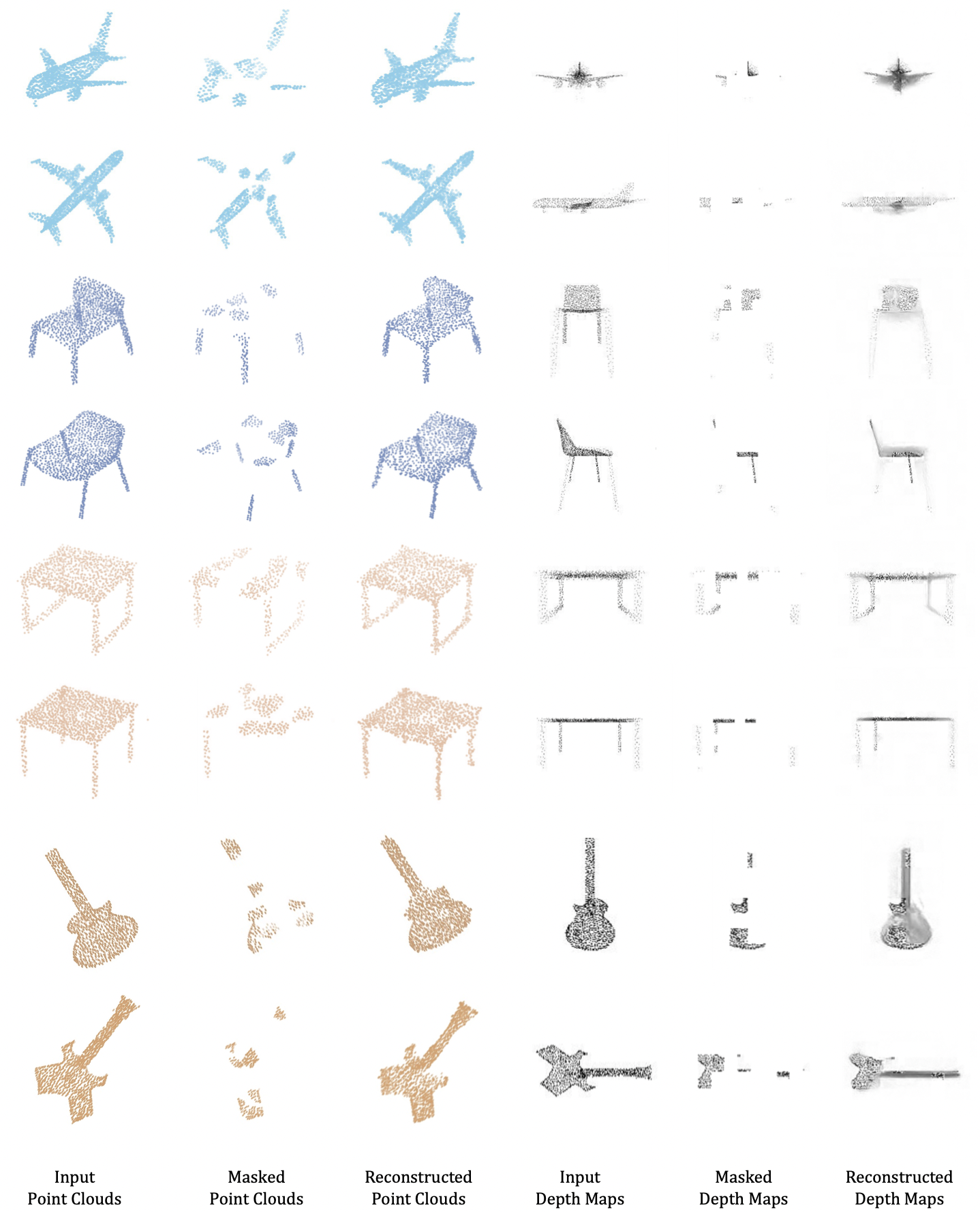
In each column of Figure 2, we show the input point clouds, the masked point clouds, the reconstructed coordinates, the input projected depth maps, the masked depth maps, and the reconstructed depth maps, respectively. As shown, with the proposed 2D-3D joint MAE pre-training and cross-modal learning strategies, Joint-MAE can well generate masked point clouds and 2D depth maps.

Local-aligned Attention.
We visualize the attention scores with local-aligned attention in Figure 3. The input 3D point clouds and projected 2D depth maps are shown in the 1st and 3rd columns. In the 2nd and 4th columns of Figure 3, the position in green means the attention weight here is zero, while orange denotes nonzero. As shown, with the local-aligned attention, the query tokens of 3D focus on the whole 3D positions and only correlative parts of 2D depth maps, which are corresponding to the valid-attention positions in Section 3.3. Meanwhile, the ignored positions in green are corresponding to the invalid-attention positions in Section 3.3. This local-aligned attention mechanism contributes to more fine-grained and intensive feature learning.
References
- Crosspoint: self-supervised cross-modal contrastive learning for 3d point cloud understanding. arXiv preprint arXiv:2203.00680. Cited by: Appendix A.
- Shapenet: an information-rich 3d model repository. arXiv preprint arXiv:1512.03012. Cited by: Appendix A.
- ConvMAE: masked convolution meets masked autoencoders. arXiv preprint arXiv:2205.03892. Cited by: Appendix A.
- Adam: a method for stochastic optimization. arXiv preprint arXiv:1412.6980. Cited by: Appendix A.
- Relation-shape convolutional neural network for point cloud analysis. In Proceedings of the IEEE/CVF Conference on Computer Vision and Pattern Recognition, pp. 8895–8904. Cited by: Appendix A.
- Revisiting point cloud classification: a new benchmark dataset and classification model on real-world data. In Proceedings of the IEEE/CVF International Conference on Computer Vision, pp. 1588–1597. Cited by: Appendix A, Table 2.
- Unsupervised point cloud pre-training via occlusion completion. In Proceedings of the IEEE/CVF International Conference on Computer Vision, pp. 9782–9792. Cited by: Appendix A.
- 3d shapenets: a deep representation for volumetric shapes. In Proceedings of the IEEE conference on computer vision and pattern recognition, pp. 1912–1920. Cited by: Appendix A, Appendix A, Table 2, Appendix B.
- A scalable active framework for region annotation in 3d shape collections. ACM Transactions on Graphics (ToG) 35 (6), pp. 1–12. Cited by: Appendix A, Table 2.
- Point-bert: pre-training 3d point cloud transformers with masked point modeling. arXiv preprint arXiv:2111.14819. Cited by: Appendix A.
- Point-m2ae: multi-scale masked autoencoders for hierarchical point cloud pre-training. arXiv preprint arXiv:2205.14401. Cited by: Appendix A.