The Athena++ Adaptive Mesh Refinement Framework: Multigrid Solvers for Self-GravityAthena++ (Athena++ development team 2021)
Abstract
We describe the implementation of multigrid solvers in the Athena++ adaptive mesh refinement (AMR) framework and their application to the solution of the Poisson equation for self-gravity. The new solvers are built on top of the AMR hierarchy and TaskList framework of Athena++ for efficient parallelization. We adopt a conservative formulation for the Laplacian operator that avoids artificial accelerations at level boundaries. Periodic, fixed, and zero-gradient boundary conditions are implemented, as well as open boundary conditions based on a multipole expansion. Hybrid parallelization using both MPI and OpenMP is adopted, and we present results of tests demonstrating the accuracy and scaling of the methods. On a uniform grid we show multigrid significantly outperforms methods based on FFTs, and requires only a small fraction of the compute time required by the (highly optimized) magnetohydrodynamic solver in Athena++. As a demonstration of the capabilities of the methods, we present the results of a test calculation of magnetized protostellar collapse on an adaptive mesh.
Keywords:
methods: numerical, gravitation, hydrodynamics, magnetohydrodynamics (MHD)I Introduction
Modeling the (magneto-)hydrodynamics of astrophysical systems often requires inclusion of self-gravity, which necessitates solution of the Poisson equation along with the MHD conservation laws. Since it is elliptic, numerical solution of the Poisson equation requires quite different methods from the explicit time integration techniques typically used for the (hyperbolic) equations of motion. In addition, when diffusive processes such as viscosity, heat conduction, Ohmic resistivity, and radiation transport in the optically-thick regime (or with the flux-limited diffusion approximation) are included in the dynamics, implicit time integration methods are often needed in order to avoid overly-restrictive constraints on the timestep. Like the solution of the Poisson equation, implicit integrators require matrix inversions that involve global communication. Therefore it is of great interest to develop efficient solvers for such non-local physical processes that are scalable to a large number of parallel processes characteristic of modern high-performance computing systems.
There are a variety of widely adopted algorithms for the solution of the Poisson equation. For uniformly-spaced Cartesian grids, a discretization in Fourier space combined with the Fast Fourier Transform (FFT) is commonly used as it is robust and efficient (Hockney & Eastwood 1988; Press et al. 2007, e.g.). However, it is not compatible with non-uniform mesh spacing and curvilinear coordinates, is most efficient only with periodic boundary conditions, and is not suitable for use with adaptive mesh refinement (AMR). When AMR is used, sparse matrix solvers like the Conjugate-Gradient method and its variants (Hockney & Eastwood 1988; Hackbusch 1994; Saad 2003, e.g.) can be adopted, but they are not trivial to implement on complicated grid structures as the matrix is irregular, and they may require robust preconditioners for efficiency. Another popular algorithm is the Tree method (Barnes & Hut 1986; Wünsch et al. 2018), which is often used in particle-based simulations. While the Tree method is suitable for isolated (open) boundary conditions, it is not trivial to combine with other boundary conditions.
In this paper, we describe the implementation of grid-based solvers for the Poisson equation of self-gravity in the Athena++ code (Stone et al. 2020) that are based on the multigrid method (Fedorenko 1962; Trottenberg et al. 2001). In particular, we focus on the so-called geometric multigrid methods, which use multiple grids with different spatial resolutions. This method applies a classical iterative solver such as the Gauss-Seidel method to damp the error at different scales coherently. By construction, multigrid is compatible with both AMR and a wide variety of different boundary conditions. Moreover, as long as communication costs are negligible, its computational complexity scales as , where is the total number of degrees of freedom. This is better than FFT and Tree algorithms, which both scale as . In this paper, we show that this difference is significant at large ; multigrid is significantly more efficient than for example, FFT methods, in this regime. We note that for the Poisson equation of self-gravity, the Fast Multipole Method (Greengard & Rokhlin 1987, FMM,) is also an efficient algorithm with .
The rest of the paper is organized as follows. In Section 2, we discuss the basics of multigrid methods. We describe our implementation of them in Section 3, and present test results in Section 4. In Section 5 we discuss and summarize our results. While the multigrid algorithms are compatible with general coordinate systems, we focus on uniformly-spaced Cartesian coordinates in this paper.
II Multigrid Solvers
In this section, we present basics of multigrid Poisson solvers. First, we describe the basic equations and their discretization in Section II.1. Next, we discuss classical iterative solvers as a foundation of the multigrid algorithms in Section II.2. Then we explain elements of the multigrid algorithms including the restriction and prolongation operators (Section II.3.1), smoothing operator and coarsest-level solver (Section II.3.2), cycling algorithms (Sections II.3.3–II.3.5), boundary conditions (Section II.3.6), and convergence criteria (Section II.3.7).
II.1 Basic Equations and Discretization
We discuss solution of the Poisson equation for self-gravity
| (1) | |||
| (2) |
where is the gravitational potential, the gravitational acceleration, the gravitational constant, and the mass density respectively. In three-dimensional (3D) Cartesian coordinates, the Laplacian operator becomes . As Athena++ uses a cell-centered discretization for the hydrodynamic quantities, we use the same discretization for and .
For simplicity, in what follows the same uniform cell spacing is adopted in all the three directions (the extension to both non-uniform or curvilinear coordinates is straightforward). In this case, the discrete form of equation (1) can be written
| (3) |
where are the cell indices in the -directions. Since Athena++ uses octree block-based AMR design, computations within each MeshBlock (domain decomposition unit in Athena++, see Section III.1) can be processed in locally-uniform grids and complexities due to AMR appear only in communications at level boundaries and refinement/derefinement procedures, as discussed in Section III.3.
It is useful to introduce some notation. We use the potential and source term vectors and in which the values of all the cells discretized with the resolution of are stored as one dimensional vector. We define the Laplacian operator discretized with , . Then eq.(3) reads
| (4) |
We define the discretized error vector and true error vector as
| (5) | |||||
| (6) |
and the defect vector as
| (7) |
where denotes the fully-converged discretized solution and is the true solution of the original Poisson equation with infinite resolution. The converged solution satisfies and . However, it should be noted that the discretized solution minimizes the true error only to the order of the truncation error, which is proportional to in the case of a second-order accurate scheme.
The error and defect vectors satisfy the defect equation:
| (8) |
The Laplacian operator is a sparse matrix and its inversion is not easy to find. Instead, we calculate an approximation to obtain the correction and then converge on the solution iteratively. We denote the approximate solution after the -th iteration as , while represents the initial guess.
II.2 Classical Iterative Solvers
To be thorough, in this section we review basic concepts of classical iterative solvers such as the Jacobi, Gauss-Seidel (GS) and Successive Over-Relaxation (SOR) methods. These methods are not very practical by themselves, but they are important as the foundation of multigrid methods. There are various derivations of these methods (Hackbusch 1994, e.g.), here we present one physically motivated (Press et al. 2007).
The Poisson equation can be reformulated as a time-dependent diffusion-like problem using the pseudo-time :
| (9) |
This is a linear diffusion equation with an additional source term. Because solutions to the Poisson equation are unique, we can start from any “initial condition” and relax to the steady state solution of equation (9) where becomes zero, and the result will then be a solution of the Poisson equation.
In order to solve this diffusion-like equation numerically, the simplest approach is to apply the standard Forward Time Centered Space (FTCS) discretization (Roache 1972; Press et al. 2007, e.g.) and use the largest possible timestep limited by the Courant-Friedrichs-Levy (CFL) condition, , where is the number of the spatial dimensions. The discretized equation in 3D is
| (10) |
where is the index of the pseudo-time or the iteration step. By repeating this procedure until reaches a steady state, we can obtain the numerical solution. This is the Jacobi method.
The timescale for the Jacobi methods to reach steady state is the diffusion time, , where is the size of the system. This estimate tells us that short wavelength structures will diffuse on the shortest time scales, but long wavelength structures take longer to diffuse away. The number of iterations required for the whole system to reach steady state can be estimated as where is the number of the cells in each dimension. As each iteration costs in 3D, the total computation complexity is . Compared to the explicit (magneto)hydrodynamic part, which is , this is very expensive.
Since we are interested only in the steady state solution of this problem, we are not strictly bound by the CFL condition and we can accelerate convergence by changing the iteration process. In the traditional (lexicographic) GS method, we replace eq.(10) with
| (11) |
Here, is used on the right hand side for already updated cells. There are advantages and disadvantages in this method. The number of iterations required for convergence is only half of the Jacobi method (Hockney & Eastwood 1988; Hackbusch 1994; Press et al. 2007), and it does not require temporary memory storage for as we can directly update the value on the same memory. However, as it is obvious from the equation, this introduces anisotropy in the iteration process, and the dependency (i.e., we cannot update until are all updated) prevents vectorization and parallelization of the code.
A variant of this is the Red-Black Gauss-Seidel (RBGS) method, in which a checkerboard pattern is used in the iteration. Here we label the even-numbered cells (i.e., = even) with red and the odd-numbered cells with black. We first update the red cells using the neighboring black cells yet to be updated, then the black cells using the red cells that are already updated.
| (12) | |||
| (13) |
This method reduces anisotropy although red and black cells are not fully equivalent. Also, this method is suitable for parallelization as all the red or black cells can be updated at the same time without dependencies. However, it should be noted that this method is still incompatible with vectorization as it requires non-unit stride access to the memory. Both GS variants still cost .
We can even accelerate convergence further by SOR. In this method, we extrapolate each iteration by the over-relaxation parameter . It can be combined with any of the classical solvers above, but in the case of the RBGS, the iteration procedure is as follows:
| (14) | |||
| (15) |
This method is convergent for . The optimal choice of depends on the problem, but
| (16) |
is known to give significant acceleration for the Poisson equation for self-gravity if the domain is cubic. This reduces the number of iterations to , and therefore the total cost is (Hockney & Eastwood 1988; Hackbusch 1994; Press et al. 2007).
It is known that SOR may not converge monotonically depending on the over-relaxation parameter and initial guess. To overcome this difficulty and improve the convergence behavior, the Chebyshev acceleration can be used. In this method, we use in the first iteration, and gradually increase it to the optimal value following a certain sequence. For further details, we refer readers to literature such as Hockney & Eastwood 1988; Press et al. 2007, as we do not use this method in our multigrid solvers.
II.3 Basics of Multigrid
The concept of multigrid methods is simple. By applying a classical iterative solver on coarse grids, long-wavelength modes damp faster as they behave as short-wavelength modes at the reduced resolution. Thus, we can use larger pseudo-timesteps on coarser grids and accelerate convergence to the steady state solution of the diffusion-like equation. The multigrid methods combine multiple layers of coarser grids consistently and damp both short- and long-wavelength modes coherently. In this section, we largely follow the discussion in Trottenberg et al. 2001.
There are two different strategies in the multigrid methods. One is the multigrid iteration (MGI) method, in which we apply the multigrid method on the finest level repeatedly to improve the solution starting from a given initial guess. The other is the full multigrid (FMG) method, which starts from the coarsest grid, and constructs the finer solutions by applying the multigrid method using the coarser solution as the initial guess. We describe the multigrid iteration method in Section II.3.3 and the full multigrid method in Section II.3.4.
In what follows, we adopt the conventional terminology used with multigrid methods. Applying a classical iterative solver on a certain level is called “smoothing”. “Restriction” means producing coarser grid data by averaging finer grid data, and “prolongation” means producing finer grid data by interpolating coarser grid data. These are basic elements of the multigrid methods, and various combinations are possible. Here, we discuss our implementation in Athena++.
Hereafter, we also use notations that is the level in the multigrid hierarchy ( is the coarsest level where the grid cannot be restricted anymore), the resolution on the level which satisfies , the Laplacian operator on level , respectively.

II.3.1 Restriction and Prolongation Operators
First, we define the restriction and prolongation operators to transfer data between different levels. As the potential and source term are discretized at cell-centers, we use the volume-weighted average for restriction and the trilinear interpolation for prolongation.
The restriction operator from level to is defined as
| (17) |
where is either the potential , the defect , or the source term , the cell volume, and are the cell indices on the coarse level corresponding to the finer cells with and its adjacent cells.
The trilinear prolongation operator from level to is defined as
| (18) |
where is either the potential or the correction . takes for if is even (i.e., the finer cell is located on the “lower” side in the coarser cell in each direction, see Figure 1), and for if is odd (the finer cell is on the “upper” side). These interpolation coefficients are derived assuming equally-spaced cubic cells in 3D Cartesian coordinates.
For the full multigrid method explained later in Section II.3.4, Trottenberg et al. 2001 recommended to use a higher-order prolongation operator to prolongate the potential, and we adopt the third-order tricubic interpolation for this purpose. It is obtained using eq.(18) but with for and even , and for and odd .
The interpolation stencils and weighting coefficients of the restriction and prolongation operators in 2D are graphically shown in Figure 1.
II.3.2 Smoothing Operator and Coarsest-Level Solver
In the multigrid algorithms, we apply a smoothing operator to reduce the error on each level. This operator receives the potential or defect vector, the linear operator and the source term vector as the input arguments, and returns the smoothed potential or defect vector. In our implementation, we adopt the RBGS smoother with the over-relaxation factor of as eqs.(14) and (15). This value of is chosen to damp high-frequency errors faster, and is different from the optimal value for the SOR solver in eq.(16) (Yavneh 1996; Trottenberg et al. 2001).
On the coarsest level, we apply the coarsest-level solver . The input arguments are the same as , and it returns the solution on the coarsest level. If the grid can be reduced to cell on the coarsest level , it is trivial to calculate the exact solution because the discretized Poisson equation (3) is reduced to
| (19) |
and all on the right hand side are given from boundary conditions. On the other hand, if the coarsest level is not reduced to a single cell but contains cells, we apply the RBGS smoother times instead, which is sufficient to obtain a good solution on the coarsest level.
II.3.3 Multigrid Iteration

Legends: Filled circles (): smoothing operations. Filled squares (): obtaining the coarsest-grid solution. Downward solid segments: restriction. Upward solid segments: prolongation. Downward dotted line: restriction operation at the beginning of the full multigrid algorithm. Upward double-solid segments: FMG prolongation.
We first describe the multigrid iteration scheme. There are various cycling procedures such as V-, W-, and F-cycles, and here we implement the simplest V-cycle in Athena++. Using pseudocode notation, one cycle of this scheme is described as follows.
Algorithm 1: V-cycle multigrid iteration
Here, and are the restriction and prolongation operators defined in Section II.3.1, and the smoothing operator and coarsest-level solver defined in Section II.3.2, respectively. We apply the smoothing operator times for presmoothing and times for postsmoothing on each level, which is called the V(M,N) cycle. While Athena++ supports , we typically use the V(1,1) cycle.
The algorithm applies recursively until it reaches the coarsest level. Note that on the coarser levels operates not on the potential itself but on the defect. This is because the self-gravity Poisson equation is linear and therefore the defect equation eq.(8) can be used instead of the Poisson equation eq.(4). This algorithm is called the multigrid correction scheme.
II.3.4 Full Multigrid
The full multigrid method (Brandt 1977) is a more sophisticated algorithm to solve the system. In this method, we start from the coarsest level where the solution can be easily calculated. The coarse-grid solution is prolongated to the finer level, and is used as an initial condition for the multigrid iteration to improve the fine-grid solution. By repeating this procedure, we can obtain a reasonably good solution once we reach the finest level. The pseudocode of this algorithm is as follows:
Algorithm 2: Full multigrid
used here is the same as in Algorithm 1. The prolongation of the solution in the full multigrid method, or the FMG prolongation, requires a higher order prolongation operator , which is explained in II.3.1. The schematic picture of the full multigrid method with the V(1,1) cycles is shown in Figure 2 (b).
It is remarkable that the full multigrid method does not require any initial guess, compared to the multigrid iteration. Instead, this algorithm fully utilizes the geometric structure to construct the initial guess for the finer levels. While we may apply more than once per level, practically one application per level is sufficient to achieve the true error of the order of the truncation error compared to an analytic solution after the full multigrid algorithm. However, the defect and the discretized error remain considerably large because the numerical solution still contains error and noises, and we need to apply additional V-cycle iterations to obtain a fully-converged solution. We discuss the error behaviors in Section IV.
II.3.5 Full Approximation Scheme
In the multigrid correction scheme presented above, the defect equation is solved when the multigrid algorithm is applied on the coarser levels. This is efficient because we need to restrict only the defect, and not the potential. This is possible because the Poisson equation and the defect equation are linear and have the same shape as in eqs (4) and (7). However, for non-linear problems, this is not satisfied. Also, when we apply the multigrid methods on the AMR hierarchy, this is not applicable because the defect is defined for a certain resolution and mathematical operations between the defects defined on different AMR levels are ill-defined.
When mesh refinement is in use (and for future extension to non-linear physical processes), we use the Full Approximation Scheme or Full Approximation Storage (Brandt 1977, FAS,). In FAS, we restrict the potential itself in addition to the defect, and solve the original equation (4) on every multigrid level. This is achieved using the following algorithm:
Algorithm 3: Full Approximation Scheme Iteration
This scheme is equivalent to the multigrid correction scheme for a linear system on uniform grid. Compared to the multigrid correction scheme, this scheme requires additional computations for restriction of the potential, calculation of the RHS, and calculation of coarse-grid correction. However, the restriction is relatively less expensive, and the other additional computations are needed only on coarser levels that have much fewer cells. Therefore, additional cost from FAS is moderate. The FAS version of the full multigrid method is obtained by replacing with in Algorithm 2.
II.3.6 Boundary Conditions
Boundary conditions are required for the smoothing operations and prolongation operations on every level of the multigrid hierarchy. The multigrid methods are compatible with various boundary conditions, and we have implemented periodic, zero-gradient, zero-fixed boundary conditions as well as isolated boundary conditions using a multipole expansion in Athena++. An interface to enroll user-defined boundary conditions is also provided. The implementation of the multipole expansion is described in Appendix A.
For the multigrid correction method, specified physical boundary conditions are applied on the finest level and zero-fixed boundary conditions are used for the defect equation on the coarser levels unless periodic boundary conditions are specified. When FAS is in use, we need to apply physical boundary conditions at every level consistently.
In Athena++, the boundary conditions are set in the ghost cells (whereas the other cells that are updated by the solvers are called “active cells”). For periodic and zero-gradient boundary conditions, the boundary values are set at cell-centers of the ghost cells. When other (e.g., isolated or fixed) boundary conditions are specified, we set the ghost cell values so that the value on the surface of the computing domain match the specified boundary values. This is because the cell-center positions of the ghost cells shift between levels.
Because the potential appears only within the Laplacian operator in the Poisson equation (1), the zero point of the potential is arbitrary. If at least one of the boundary conditions contains a fixed value, it sets the zero point. For the multipole expansion, it is natural to set it to zero at infinity. If all the boundary conditions do not set any fixed value (e.g., all the boundaries are periodic or zero-gradient), a Poisson solver cannot find the zero point by itself. In this case, we use the deviations from the averages of the source function and the potential, and where is the volume average of . The Poisson equation retains the same shape as , but now we set the potential zero point to zero so that the average of the potential is .
II.3.7 Convergence Criterion
In Athena++, two iteration modes are available. In the “FMG” (Full MultiGrid) mode, the full multigrid method is used first, and then V-cycle iterations are applied to improve the solution. In the “MGI” (MultiGrid Iteration) mode, one has to provide an initial guess and V-cycle iterations are applied repeatedly. In practical hydrodynamic simulations, one can use the potential from the previous timestep as the initial guess, but usually it is not as good as the numerical solution after one sweep of the full multigrid method. In general, we recommend the FMG mode because it requires no initial guess and performs better in most cases as shown in Section IV.
In both modes, the V-cycle iteration is repeated until a certain convergence threshold is met or until convergence saturates and the error reduction stalls. As the discretized error (5) and true error (6) are unknown beforehand, we use the defect (7) as the convergence threshold. Specifically, we use the volume-averaged root-mean-square of the defect :
| (20) | |||||
| (21) | |||||
where is the volume of each cell and the summation is over all the cells in the computing domain. Here, the defect is calculated on the finest (unrestricted) level. Once this value gets smaller than a user-specified threshold, the code stops. A user has to carefully specify a resonably-small threshold value for this, or set it to zero to repeat the iteration until convergence saturates. Alternatively, one can use a fixed number of iterations if it is possible to determine the number of iterations needed to achieve demanded accuracy. Because the demanded accuracy and corresponding defect threshold depend on problems, there is no threshold value that can be used universally. We recommend users to try a few different parameters to determine the convergence threshold before starting a production run.
III Numerical Implementation
In this section, we first review relevant features of the Athena++ code briefly (Section III.1). Then we present our implementations of the multigrid solvers on uniform grids (Section III.2) and with AMR (Section III.3). Lastly, we discuss the cost of the multigrid solvers in Section III.4.
III.1 Brief Review of Athena++
Athena++ (Stone et al. 2020) is a public AMR framework supporting various physical processes and features for astrophysical applications, including non-uniform mesh spacing, Cartesian and curvilinear coordinates, static and adaptive mesh refinement, magnetohydrodynamics (MHD), special and general relativity (White et al. 2016), chemical reactions, general equation-of-states (Coleman 2020), particles (Yang et al. in prep.), shearing box and orbital advection (Ono et al. in prep.), non-ideal MHD effects and other diffusion processes, as well as other physics. Beyond the public version, various extensions such as cosmic-ray transport (Armillotta et al. 2021), time-dependent radiation transport (Jiang 2021), post-processing general relativistic radiation transport (White 2022) and full general relativity (Daszuta et al. 2021), are being actively developed in the community as well. For self-gravity, there is already an implementation based on FFTs for uniform grids (developed by C.-G. Kim). The code is publicly available on GitHub, and documentation and a tutorial are available on the website11 1 https://www.athena-astro.app/.
Athena++ is parallelized using the standard domain decomposition technique using MPI and OpenMP. The computing domain is split into units called MeshBlocks, each of the same logical size (i.e., containing the same number of cells). In Athena++, MPI processes and OpenMP threads are almost equivalent; each process or thread owns one or more MeshBlocks. Each MeshBlock has additional ghost cells at each boundaries for communication between MeshBlocks and also for physical boundary conditions. The ghost cell data are transferred via MPI messages or memory copy depending on they are on the same MPI process or not.
Athena++ adopts an octree block-based AMR design. In this design, a MeshBlock is not only the domain decomposition unit for parallelization but also the unit for mesh refinement. When a MeshBlock is refined, it is split into eight finer MeshBlocks in 3D. Neighboring MeshBlocks are also refined so that only MeshBlocks on the same level or one level different contact each other. This design is computationally efficient, because all the MeshBlocks are logically uniform grids of the same shape, and highly-optimized codes for uniform grids can be applied. The design also works well for parallelization because only a few simple patterns for communication between MeshBlocks need to be considered. We use the Z-ordering to assign globally unique IDs to MeshBlocks, and distribute them as evenly as possible for parallelization.
One of unique designs of Athena++ is dynamical scheduling using a TaskList. The simulation program is split into small Tasks with associated dependencies, which are then assembled into a TaskList. Normally Tasks are processed sequentially from the beginning of a TaskList, but when the code has to wait for communication associated with a particular Task to arrive, it automatically processes the next Tasks in the TaskList that do not depend on the communication. This enables overlapping of computation and communication automatically. In addition, as this design separates logic within each physics module and relation between modules, it improves flexibility and modularity of the design.
Athena++ uses uniform timestepping even when AMR is in use. This means that all MeshBlocks on all levels share the same timestep. While this methods does not minimize the number of operations, it often is the most efficient because it does not require complicated scheduling and load-balancing logic nor synchronization between AMR levels, and parallelization is straightforward. Moreover, non-local physics such as self-gravity and radiation transport with an implicit time integrator are captured more accurately since the solution at every level is at the same time and temporal interpolation is not necessary. Thus, the uniform timestepping as adopted in Athena++ is advantageous for applications involving non-local physics. For complete details of Athena++, we refer readers to the method paper (Stone et al. 2020). In particular, the design of the AMR framework is discussed in Section 2.1 and the TaskList implementation is in Section 2.5.
III.2 Uniform Grid
We first describe our implementation of the multigrid methods on uniform grids in this section. Our implementation does not depend on any external library (except for MPI), and the code is written in C++11.
III.2.1 Multigrid Hierarchy and Data Structure
We decompose the computational domain using the same MeshBlocks as in the main (hydrodynamics or MHD) part. Because we apply the restriction and prolongation operators on each MeshBlock, each MeshBlock has to be logically cubic and the number of active cells in each direction must be power of two, i.e., . This is more restrictive than the AMR of Athena++. However, there is no limitation in the number of MeshBlocks in each direction. We define the coarsest level where the grid cannot be restricted anymore as level 0. Let correspond to the numbers of cells in each direction on level . If the number of cells on level 0 is , then . There is a certain level where the number of the cells matches the number of the MeshBlocks . In total there are levels, and the total number of cells in each direction is , where is the number of MeshBlocks in each direction.
The potential, source function and defect on levels from to are stored as multi-dimensional arrays in Multigrid class in each MeshBlock. On the other hand, those data on levels from to are stored in a separate Multigrid class, which we call RootGrids. In addition to the active cells, ghost cells are allocated on each side of the Multigrids for communication with neighboring Multigrids. For self-gravity, we need only one layer of the ghost cells, . When FAS is in use, additional storage is allocated for the restricted potential on coarser levels. The data on level are stored both in RootGrids and Multigrid for communication and synchronization between these objects. Note that each Multigrid object contains only cell on level . Hereafter, we refer levels to as RootGrid levels and to as MeshBlock levels.
III.2.2 V-Cycle Algorithm on Uniform Grid
In the V-cycle algorithm, we start the iteration procedure from the finest level, whose data are stored in Multigrids. To start up the algorithm, the source function is calculated using the mass density loaded from the MeshBlocks, and the initial guess is loaded into the potential data.
As in Algorithm 1, each iteration starts with pre-smoothing using the RBGS smoother. We then calculate the defect , restrict and transfer it to the coarser level. This procedure is repeated recursively until it reaches level , where each MeshBlock is restricted to cell and cannot be restricted anymore. At this point, the data on level are collected from all the Multigrids and transferred to the array on level in RootGrids. Then, the recursion continues to the RootGrid levels until it reaches the coarsest level . The coarsest level solution is easily obtained using the coarsest-level solver described in SectionII.3.2 because there are only a few degrees of freedom.
Then, the correction on the coarse level is prolongated into the finer level. After adding the correction, we apply the RBGS smoother for post-smoothing. This procedure is repeated until it reaches level where the data are transferred from RootGrids to Multigrids, then continues to the finest level . This completes one iteration of the V-cycle algorithm.
After each V-cycle iteration, the average defect (20) is computed and compared with a given convergence threshold. Once the convergence criterion discussed in Section II.3.7 is satisfied, the algorithm is completed and returns the potential as the result. The potential is then used in the hydrodynamics or MHD part to calculate the gravitational acceleration.
The logic remains almost the same even with FAS enabled. In this case, the potential is also restricted along with the defect, and additional computations of the RHS and coarse-grid correction are performed accordingly.
III.2.3 Time Integration of Hydrodynamic Source Terms
The time integration of the hydrodynamics or MHD part is done in the main integrator of Athena++, which is either the second-order van-Leer, second-order Runge-Kutta or third-order Runge-Kutta. The integration procedure is processed using TaskList, but the multigrid solver is implemented using a separate TaskList from the main integrator. In every substep, we load the density given from the time integrator to the multigrid module, run the multigrid solver, pass the potential back to the hydrodynamics/MHD module, and run the main integrator. This is not the most cost-effective implementation as it requires a multigrid solve for each substep of the integrator, but it is simple and compatible with any time integrator.
The momentum and energy source terms by the gravitational force are calculated using the cell-centered source term scheme (Mullen et al. 2021). For example, the momentum source term in the -direction is
and the energy source term is
where , etc. is the mass flux at the cell interface returned from a Riemann Solver. This implementation is curl-free, contrary to the implementation using the gravitational flux (Jiang et al. 2013, e.g.)22 2 A curl-free implementation based on the gravitational flux is proposed in Mullen et al. 2021. On the other hand, for time integration, we simply use one of the standard integrators in Athena++ and we do not use the conservative scheme for the energy term proposed in Mullen et al. 2021. Therefore, our scheme does not exactly conserve the energy, only to the accuracy of the scheme. It should be noted that both momentum and energy are not conserved exactly to the round-off error because there is non-zero residual in the potential obtained with the multigrid solver in general.
Technically, it is possible to combine the self-gravity TaskList and hydrodynamics/MHD TaskList and maximize communication-computation overlapping. The reason why we implement the self-gravity as a separate TaskList from the main integrator is partly for simplicity, but also for future extension to heterogeneous parallelization, in which some nodes process self-gravity while other nodes work on other physical processes. Because the multigrid solver is less scalable than the MHD solver as shown later in Section IV, such an advanced parallelization technique could be useful in the future to improve the overall parallelization efficiency.
III.2.4 FMG Algorithm on Uniform Grid
The implementation of FMG is straightforward on top of the V-cycle algorithm. First, the source function is restricted from the finest levels to the coarsest levels and stored on each level. Then, we start the algorithm from the coarsest level. On the coarsest level, the solution is obtained either analytically or using a few sweeps of the iterative solver. Then, this solution is prolongated using the third-order tricubic interpolation to the finer level. Using the prolongated solution as the initial guess, the V-cycle algorithm is applied to improve the solution on this level. We repeat this procedure until it reaches the finest level, as shown in Figure 2 (b). Once the solution on the finest level is obtained, we apply the V-cycle repeatedly to improve its accuracy until the convergence criterion is satisfied.
III.2.5 Parallelization
In order to run large-scale simulations on modern supercomputers, parallelization is of crucial importance. Because parallelization of FMG is trivial once the V-cycle is parallelized, we describe the parallelization of the V-cycle algorithm here.
As in the hydrodynamic/MHD part in Athena++, the multigrid solver is parallelized using both MPI and OpenMP. When parallelization is enabled, each MPI process (or OpenMP thread in case OpenMP or hybrid parallelization is in use) owns one or more MeshBlocks and associated Multigrids. The data on the MeshBlock levels are stored in Multigrids and distributed to each process. Parallelization in the MeshBlock levels is similar to the hydrodynamic/MHD part. The data on the boundaries are transferred to and from neighboring Multigrids through the ghost cells before the smoothing and prolongation operations. For the RBGS smoother, the boundaries are communicated before each sweep of red and black. Using TaskList, computations and communications are automatically overlapped.
Once the algorithm reaches the transition level where each Multigrid is reduced to a single cell, the data on this level are collected and transferred to RootGrids on every MPI rank using MPI_Allgather33 3 Logically, this implementation is the same as collecting the data into one MPI rank with MPI_Gather, processing the RootGrids, then distributing the data back to Multigrids with MPI_Scatter. However, we chose our implementation considering that one MPI_Allgather requires less synchronization than the combination of MPI_Gather and MPI_Scatter.. Then, every rank performs the multigrid algorithm on the RootGrid levels. Once it comes back to level , then the data are transferred to each Multigrid. Then, again each MPI process or OpenMP thread calculates the assigned Multigrids.

III.3 Mesh Refinement
We do not discuss generation, destruction and load-balancing of MeshBlocks here because these processes are unchanged by the addition of multigrid, and are controlled by teh AMR framework of Athena++. For details, see the method paper (Stone et al. 2020).
There are, however, two major changes to the multigrid algorithm itself with mesh refinement. One is manipulation of the refined Multigrids on coarse levels, and the other is boundary communication between neighboring Multigrids on different levels.
III.3.1 V-Cycle Algorithm on AMR Hierarchy
An example of the multigrid operations on an AMR hierarchy is shown in Figure 3. Compared to the uniform grid, there are additional levels where refined MeshBlocks are inserted as shown in Panels (c) and (d). We refer these levels as Octet levels. Because of the octree AMR design of Athena++, a MeshBlock is always refined into a set of finer MeshBlocks in 3D ( in 2D). We call this set Octet in Athena++, and we perform the smoothing, restriction and prolongation operations on each Octet. Similar to Multigrids, the potential, source function and defect data are allocated in each Octet object, which contains cells and ghost cells on each side for boundary communications. The relations between the finer and coarser MeshBlocks/Octets as well as the connections between neighboring MeshBlocks/Octets are calculated using the MeshBlockTree facility in Athena++.
When AMR is enabled, FAS is used as discussed in Section II.3.5. The algorithm on the MeshBlock levels is not very different from the uniform grid case. Starting from the finest level, it goes up the multigrid levels toward the coarser levels (Figure 3 (f) to (e)). The level boundaries are described in the next section.
When it reaches the level where each MeshBlock is reduced to a single cell (Figure 3 (d)), the data on Multigrids that are not refined are directly transferred to the RootGrids, while the data on Multigrds generated by refinement are transferred to corresponding cells in Octets. Then we apply smoothing on the Octets on the finest level and restrict the them to the coarser levels (Figure 3 (d) to (b)). For this smoothing operation, the boundaries contacting other Octets on the same level are actively updated, while the boundaries facing the coarser level are given as fixed boundary values prolongated from the coarser level. Once all the Octet levels are removed by repeating this procedure, the data are transferred to the corresponding cells in the RootGrids. Then, the algorithm continues toward the coarsest level as in the uniform grid case (Figure 3 (b) to (a)).
Once it reaches the coarsest level, the solution on the coarsest level is calculated in the same way as in the uniform grid case. Then the algorithm goes back to the finer levels by prolongation (Figure 3 (a) to (b)). When it reaches the first Octet level, the Octets on the first level are generated by prolongating the corresponding cells on the RootGrids, and then the smoothing operator is applied on the newly generated Octets (Figure 3 (c)). This procedure is repeated toward the finer Octet levels (Figure 3 (c) to (d)). When it comes back to the MeshBlock level, the data are transferred to Multigrids, and then they are prolongated and smoothed recursively until it reaches the finest level (Figure 3 (e) to (f)). This completes one V-cycle iteration on an AMR hierarchy.
We note that in some implementations of self-gravity solvers described in the literature (Kravtsov et al. 1997; Guillet & Teyssier 2011; Bryan et al. 2014; Ramsey et al. 2018, e.g.), each refined level is solved separately using the coarser level data as boundary conditions. However, such a level-by-level or block-by-block approach is not self-consistent as the coarse level solutions do not incorporate small-scale structure on the finer levels, which then implies the finer level solutions are not accurate because the boundary conditions obtained from the coarser levels are not correct. In contrast, the iteration algorithm on AMR meshes used here solves the Poisson equation across all the refinement levels consistently. We present a rough comparison between these approaches in Appendix B.
Since FMG is built on top of the V-cycle algorithm, its implementation is straightforward once the V-cycle with mesh refinement is implemented. Parallelization of the multigrid algorithm with mesh refinement is similar to the uniform grid case.
Our iteration algorithm on AMR is slightly different from what is proposed in Trottenberg et al. 2001. In the first part of the V-cycle algorithm, we restrict all the Multigrids until they are reduced to a single cell and then remove them. In contrast, with the method of Trottenberg et al. 2001, locally-refined Multigrids are removed first. We chose this design because our implementation can maintain load balance better, since the number of Multigrids remains the same until it reaches the Octet levels.

III.3.2 Level Boundaries
On the MeshBlock and Octet levels, Multigrids and Octets on different levels contact each other. In this section, we refer MeshBlocks and Octets as Blocks as the boundary operations are the same. It is of crucial importance for the AMR multigrid solver to consistently connect such level boundaries. In Athena++, this is done by properly computing the ghost cell values at level boundaries. For this purpose, we adopt a method similar to those proposed in Feng et al. 2018. We use two types of level boundaries. One adopts a conservative formulation and is used for the boundary communications before smoothing operations and force calculation, while the other is a simpler “normal” level boundary used before the prolongation operations. While the hydrodynamic/MHD part of Athena++ requires two or more layers of the ghost cells (depending on the spatial order of the reconstruction methods), the second-order multigrid solver implemented here uses only one ghost cell layer even with AMR, because the discretized Laplacian operator (3) spans a seven-point stencil in 3D.
Conservative Formulation. In order for the Laplacian operator to be accurate at level boundaries, the gravitational acceleration at cell interfaces at level boundaries must be the same for both the fine and coarse grids. For example, on the left surface in the -direction, the following condition must be satisfied:
| (23) |
where and are the -indexes of the first cells on the coarser and finer levels, and the - and -indexes of the corresponding cells on the coarser and finer levels, the resolution on the finer level. Note that this operation as well as the following computations should be replaced with area-weighted average or appropriately weighted interpolations if the grid spacing is not uniform and isotropic. Note that the constraint expressed by equation (23) enforces the truncation error in the calculation of the gradient to be divergence-free, which is equivalent to preventing an artificial or “fake” mass at the boundary. Note that the AMR algorithms used to integrate the MHD equations also require flux-corrections at fine/coarse boundaries in order to conserve quantities such as mass and momentum, however with multigrid it is possible to adopt the appropriate difference formulae that satisfies conservation by its construction without any additional correction steps.
As an example, let us consider a configuration illustrated in Figure 4 (a) and explain the level boundaries contacting in the -direction at and , but generalization to other configuration is straightforward. Here after the cell indices on the coarser and finer levels are represented using the capital and lowercase letters, and without any specific description, a coarse cell at corresponds to finer cells with indices and adjacent cells.
First, we restrict the potential in the first active cells on the finer level facing the coarser neighbor (open squares) using the area weighted average,
and send them to the coarser neighbor (black plus symbols). At the same time, we send the potential in the first active cells on the coarser level to the finer neighbor. The first active cells from the neighbors contacting on edges and corners are also sent to the finer neighbor as we need them later to calculate the transverse gradients. If these edge or corner neighbors are on the same level as the finer neighbor, we send restricted values as well (e.g. the filled circle at obtained by restricting the adjacent open squares and triangles).
Once the communications are completed, on the process which owns the finer Block, we calculate the transverse gradients on the coarser level:
| (24) |
Using these gradients, we interpolate the potential to the points aligned to the cell centers of the finer level (black crosses):
| (25) |
Note that the average potential of these four points is equal to the coarse potential . Then, by interpolation between these points (black crosses) and the first active cells (white squares), we calculate the ghost cell values on the finer Block (filled squares)
| (26) |
where and are 0 or 1. At the same time, on the process which owns the coarser Block, we calculate the ghost values at the cell centers (filled circles) by extrapolating the gradient between the active cell centers (open circles) and the points received from the finer Block (black plus symbols):
| (27) |
The gradients used in the interpolation on the finer level (26) are calculated between the black crosses and open squares. On the other hand, the gradients used in the extrapolation on the coarser level (27) are calculated between the open circles and black plus symbols. Across each cell interface, the average of the gradients on the finer level matches the gradient on the coarser level. Therefore, these ghost values satisfy the mass conservation condition (23). In addition, this scheme requires minimum communications, only one set of the communications which are mutually independent.
When a coarser cell is facing more than one finer Blocks, prolongated ghost cells contacting the finer neighbors have multiple values for each finer neighbor. Such cells are called double (or triple if it is on the corner facing three finer neighbors) ghost cells (the orange square in Figure 4). They do not cause any problem for the smoothing operations and force calculations, but we need a different method for boundary conditions for the prolongation operation, as the prolongation requires a consistent and unique value even in double ghost cells.
Although we use the same RBGS smoother even with AMR, it should be noted that the red-and-black pattern cannot be satisfied at level boundaries because one coarse cell faces four finer cells, which include two red and two black cells. We simply update all the ghost cells at the level boundaries after each smoothing operation.
Feng et al. 2018 used a different method in order to calculate the ghost cell values of the finer Block (filled squares). In their stencil (see Figure 4 in Feng et al. 2018), extrapolation of the transverse gradients of the first active cells (open squares) in the finer Block is used instead of the interpolation in eq.(24). In contrast, our scheme (24-26) corresponds to the stencil in their paper. We find some cases where the stencil behaves better, because the extrapolated transverse gradients used in the stencil can be considerably different from actual ones.
Normal Interpolation. For the prolongation operations including the higher order interpolation in the FMG algorithm, we adopt a different boundary condition. This is because we need to fill the ghost cells not only from the face neighbors but also the edge and corner neighbors, as the prolongation requires a larger stencil ( cells) than the Laplacian operator (Figure 1). For this purpose, we simply calculate the ghost cells at the level boundaries using the same restriction and prolongation operations in the multigrid algorithm itself because the boundary conditions for the prolongation do not require the conservative formulation described above.
The interpolation procedure is illustrated in Figure 4 (b). For the ghost cells on the coarser Blocks, the active cells facing the level boundaries (open squares) on the finer level are restricted using (17), then sent to the ghost cells in the coarser Blocks (filled circles). At the same time, the active cells on the coarser Blocks facing the finer level (open circles) are sent to the finer Blocks. If some of the neighbors needed for the prolongation are on the finer level, those data are also restricted (filled circles). These data on the coarser level are prolongated using the trilinear prolongation operator (18, blue arrows) into the ghost cells in the finer Blocks (filled squares). Again, these boundary communications are designed so that one set of the mutually-independent communications are required. Note that we use the trilinear prolongation even for the boundary conditions for the FMG prolongation because the trilinear prolongation does not need additional ghost cells, and also because we still can maintain the overall second-order accuracy with it.
III.4 Cost of Multigrid
The majority of the computing cost of the multigrid methods come from the smoothing, restriction and prolongation operations, which are proportional to the total number of the cells. As the coarser level contains one-eighth cells of the finer level, the total number of the operations of one V-cycle is proportional to . Therefore, the computational complexity of our multigrid algorithms per sweep is . As the multigrid methods reduce the errors at all the wavelengths coherently, the number of iterations required to achieve a given accuracy does not depend on the number of the cells. Thus, the total computational cost of the multigird algorithms is also or . This is the advantage of the multigrid algorithms compared to FFT which is , and to classical iterative solvers such as SOR which is .
In order to perform very large simulations, the parallel scalability of the algorithm is of great importance and interest. In particular, we here focus on weak scaling, where we increase the size of the simulation proportional to the number of parallel processes and keep the load per each process constant. As the computational complexity of the multigrid algorithms is , the multigrid methods are expected to achieve good parallel scaling as long as the overhead of communications is not significant and cost of the RootGrids and Octet levels is subdominant, as these parts are not fully parallelized in our implementation. The computational cost of the RootGrid and Octetlevels should be relatively small because the degrees of freedom are only as large as the number of the Multigrids. However, for massively parallel simulations particularly with AMR, the RootGrids can have significant computational load and it may degrade the parallel performance if only one CPU core is used there. An additional layer of parallelization may be needed to improve the parallel performance in such cases, but we leave it for future work.
On uniform grids, the cost of the RootGrids is proportional to the number of the MeshBlocks, or , while the cost of the MeshBlocks levels is where is the number of the cells per MeshBlock in each direction. Therefore, it is favorable for parallel performance to use larger MeshBlocks on uniform grids. Roughly speaking, it is difficult to achieve good parallel performance if is larger than . For AMR, the best MeshBlock configuration depends on problems and the size of MeshBlocks should be carefully selected so that an optimal balance between the performance and grid flexibility is achieved. We demonstrate the parallel performance of our multigrid solver in Section IV.
IV Test Results
In order to demonstrate the accuracy and performance of our multigrid solver, we show results of some test problems. First we demonstrate accuracy and performance of the gravity solvers on uniform grids (Section IV.1) and with AMR (Section IV.2). We also discuss the Jeans wave test in which hydrodynamics and self-gravity are coupled (Section IV.3). Lastly, we show collapse of a magnetized molecular cloud in Section IV.4 as a practical example of self-gravitational MHD simulations with AMR.. All the performance tests are carried out on Cray XC50 Supercomputer at Center of Computational Astrophysics, National Astronomical Observatory of Japan. Each node is equipped with two Intel Xeon Skylake 6148 processors (2.4GHz, 40 cores per node) and connected with the Aries interconnect. We compile the code using Intel C++ Compiler 2018 and Cray MPI version 7.7.0, and we report results with flat MPI parallelization.
IV.1 Uniform Grid: Sinusoidal Waves
We first demonstrate the behavior of the code using a simple static problem. Here we solve the gravitational potential for a sinusoidal density distribution in a periodic box. The computational domain size is and all the boundary conditions are periodic. The density is set up overlaying sinusoidal waves in the three dimensions,
| (28) |
where is the background density and is the amplitude. This problem has an analytic solution:
| (29) |
where we set the zero point of the potential to as discussed in Section II.3.6. In this test, we set and and take the unit of .
IV.1.1 Convergence
In order to see the convergence behavior of the FMG and MGI algorithms, we perform this test with a fixed box size of changing the resolution from to . For MGI, we use as the initial guess, which is naïve but not very poor in this case. We measure three quantities as functions of the number of the iterations: the error compared to the pointwise analytic solution (equation 6), the error compared to the fully-converged discretized solution (equation 5), and the defect (equation 7). It should be noted that the errors and the defect have different dimensions. We use the solution after 20 iterations as the fully-converged discretized solution. The results are shown in Figure 5.
As shown in Panel (a), all the algorithms quickly reach saturation against the analytic solution. This is because the numerical solutions converge not to the analytic solution corresponding to infinite resolution but to the exact discretized solution for the finite resolution, as shown in Panel (b) (Moon et al. 2019, see also). In all the algorithms, each V-cycle iteration reduces the error (b) and defect (c) by the convergence factor , which is consistent with that obtained in literature (Yavneh 1996, e.g.). Depending on the resolution and algorithms, 10–15 iterations are needed to reach fully converged solutions.
When the numerical solutions reach convergence, both FMG and MGI achieve second-order accuracy as shown in Panel (d). is the number of the additional V-cycle iterations after the first FMG sweep. It is remarkable that the first FMG sweep without additional V-cycle iterations can achieve the error as small as the truncation error (in this particular problem, the error after the first FMG sweep is smaller than the error of the converged solution). However, because the solution after the first FMG sweep still contains high-frequency noises originating from the RBGS iteration pattern, it is recommended to apply a few V-cycle iterations which can damp the high-frequency noises quickly. On the other hand, it is not necessary to repeat iterations until the defect reaches saturation. In practice, a few additional V-cycles should be enough to achieve sufficiently small potential error, e.g. .
The cost of one FMG sweep is comparable to two V-cycle iterations because the operations on the finest level dominate the cost (Figure 2). Unless the initial guess is very close to the true solution, MGI costs more than FMG to reach the same error level. As shown in Figure 5, FMG is more effective in higher resolutions. In practice, we can use the potential from the last timestep as the initial guess in hydrodynamic simulations. However, we find that it is usually insufficient and FMG almost always outperforms MGI.
IV.1.2 Performance
To demonstrate the parallel performance of our implementations, we perform weak-scaling tests using the same problem. We show the results of FMG with and , and compare the results with the performance of Athena++’s MHD solver and gravity solver using FFT. Here we fix the size of each MeshBlock and increase the domain size as we increase the number of parallel processes. As we measure the scaling using whole nodes with 40 cores, the computational domain is not always a cube but generally a cuboid, which is not necessarily an optimal configuration for the multigrid solvers because the coarsest level cannot be always reduced to a single cell. It is also not optimal for FFT because it works best if the number of cells is power of two. Nevertheless, this configuration is close to practical use cases.
The results of the weak scaling test are shown in Figure 6. Because the performance of the multigrid solver is mainly limited by the memory bandwidth, it is inevitable that the performance declines as the number of processes increases within one node. Beyond one node, the runs with larger MeshBlocks scale better, and scalabilities between 2 nodes and 200 nodes are 89.6%, 73.2%, 45.7% with MeshBlocks of , , cells for FMG one sweep and 92.9%, 78.8%, 56.3% for FMG with 10 V-cycles. We also run a test with 8 MeshBlocks of cells, where the total computation size is the same as the case while the performance is similar to the case. We find that the performance of the multigrid solver fluctuates considerably depending on conditions of the network such as the distance between allocated nodes on the network and loads by other applications sharing the network. This is because the solver transfers many small messages and therefore it is sensitive to the network latency and bandwidth. The numbers reported here are the averages of the ten best results out of 100 runs. We tend to get poor performance when the supercomputer is crowded, and it is up to slower in the worst cases. FMG with 10 V-cycles costs about 5–6 times more than one sweep of FMG because one sweep of FMG costs about two V-cycle iteration as discussed in the previous section.
It is interesting to compare the performance of the multigrid solver to the FFT solver. As shown in the Figure, the FFT solver is not very scalable and the performance degrades with larger simulation sizes. This is not because there is a problem in the implementation of the FFT solver in Athena++, but it is actually a natural consequence because FFT’s cost is intrinsically . Therefore, the multigrid solver outperforms the FFT solver in practical use cases, particularly for massively parallel simulations.
Compared to the MHD solver using the same MeshBlocks of , one FMG sweep costs only about 15% while FMG with 10 V-cycles costs about 70% of the MHD solver. Considering that we need to call the gravity solver twice per timestep with the second-order time integrator, these results indicate that the cost of the gravity solver on uniform grids is considerably smaller if only one FMG sweep is used, and it is comparable to MHD even with 10 V-cycles. In practical use cases, we need to apply the V-cycle iterations only a few times, therefore the self-gravity should cost only a fraction of the MHD solver. The parallel scalability of our gravity solver is not perfect because the self-gravity intrinsically requires extensive global communications, but these results demonstrate that our solver is highly efficient and enables large-scale self-gravitational hydrodynamic simulations.
IV.2 Mesh Refinement: Binary Potential
Next, we demonstrate the accuracy and performance of our multigrid solvers with AMR. As a non-trivial but simple static problem, we solve the potential of an unequal-mass binary system. We put the primary star with the mass of at and the secondary with at . Each star is modeled as a uniform sphere with the radius of . In order to make the density distribution near the surface smooth, we split each cell into subcells and calculate the cell density by taking the average over the subcells. The isolated boundary conditions using the multipole expansion up to hexadecapoles are applied on all the boundaries. The analytic solution of this problem is given as follows:
The size of the computing domain is , and we place refined grids with times higher resolution at up to self-similarly.
IV.2.1 Convergence
We perform a similar resolution study as in Section IV.1.1. We change the resolution of the root grid from to . The maximum resolution on the finest level is 16 times higher than that of the root grid. For lower resolutions, the binary system is completely unresolved on the root grid. Again we use as the initial guess for MGI, which is very poor in this case. We use the solution after 40 iterations as the fully-converged discretized solution. The results are shown in Figure 7. In this test, because the potential in this problem drastically varies in space, we measure the potential error normalized by the analytic solution instead of the potential itself as in the previous test:
| (30) | |||||
| (31) |
where is the numerical solution after the -th V-cycle iteration, the fully-converged discretized solution and the analytic solution, respectively. The root-mean-square of the errors plotted in Figure 7 can be considered as the typical fractional error. On the other hand, we plot the defect itself and it is not normalized.
Overall, the solvers behave similarly as in the uniform grid case, and they achieve second-order accuracy as shown in Panel (d). However, the detail of the convergence behavior is different. While FMG quickly reach saturation against the analytic solution after only a few iterations, MGI takes considerably more iterations as the initial guess is not good (Panel (a)). The error compared to the fully-converged discretized solution (b) and the defect (c) exhibit the detailed behaviors of the algorithms. Initially, FMG converges quickly with , but later it slows down to . MGI shows a similar trend, but its initial convergence is slower than FMG. This is because the first sweep of FMG gives a good initial guess globally compared to the naïve guess used in MGI. These results clearly demonstrate the superiority of FMG over MGI.
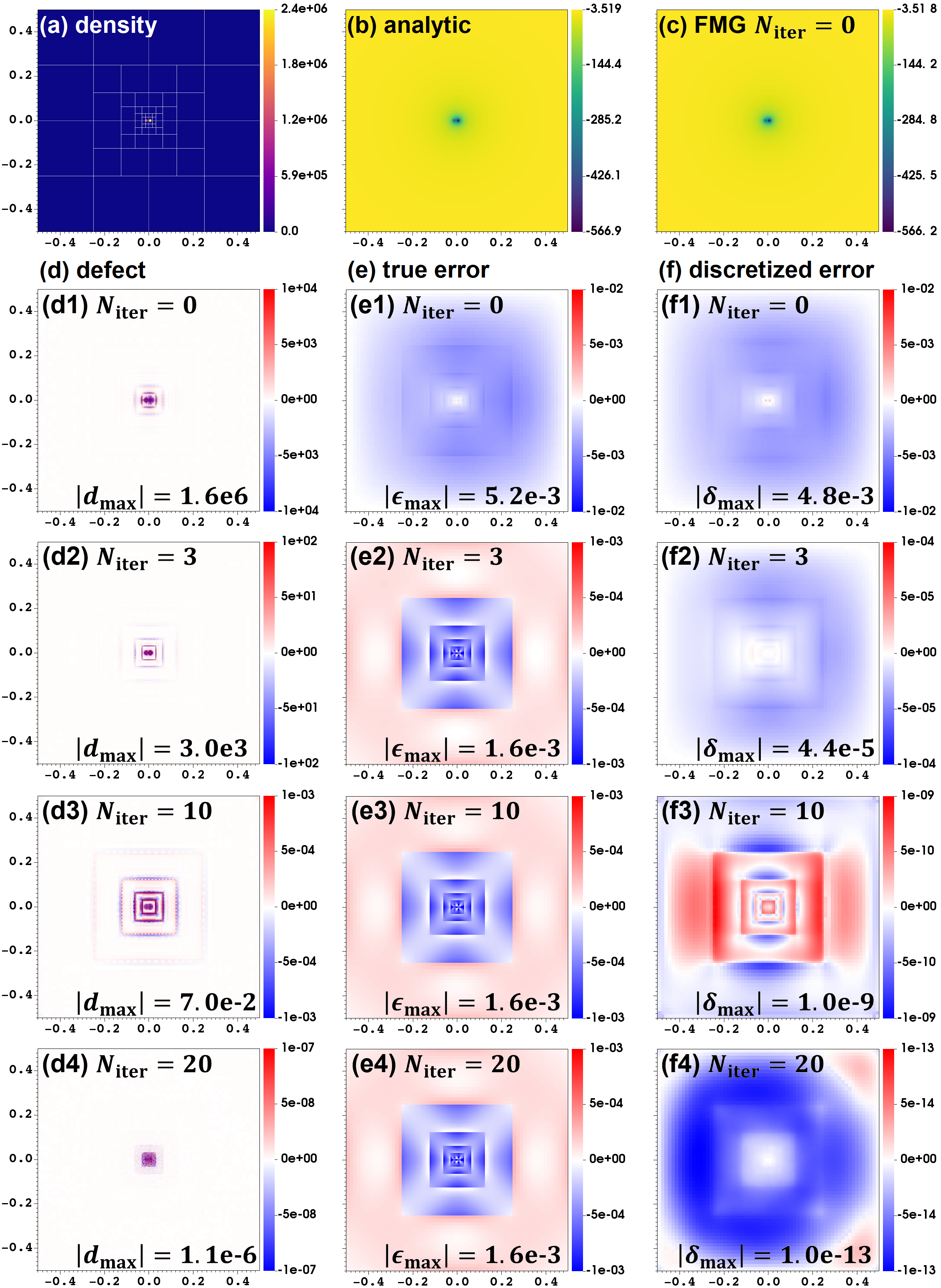
To understand the convergence behavior, we show the distributions of the errors and defect of FMG in Figure 8. The checker-board pattern seen in the defect originates from the RBGS smoothing operation. The error compared to the analytic solution quickly converges and it is small enough even after the first FMG sweep (Panels e1–e4). During the initial fast converging phase, the error to the fully converged solution and defect are reduced globally (Panels d1–d2 and f1–f2). In the later phase, the persisting errors at the level boundaries cause the slower convergence (Panels d3 and f3), but eventually the errors and defect are sufficiently reduced and approach the fully-converged solution (Panels d3 and f3). As seen in Panels (b), (c) and (e), the potential error against the analytic solution declines quickly even with a few iterations. Therefore, again, a few additional V-cycles should be enough to achieve sufficiently small error in practice.
IV.2.2 Performance
We measure the parallel performance of our multigrid solver using the same problem. We measure strong scaling where the computational load of the whole simulation is fixed and weak scaling where the computational load per process is fixed.
In order to simulate typical use cases with AMR, we apply V-cycle iterations three times after the first FMG sweep. To see the performance with different MeshBlock sizes, we run the test calculations with and cells per MeshBlock. In this test, we use only 36 cores per node so that the number of the Multigrids can be evenly divisible. In the strong scaling test, we set up the root grid of with MeshBlocks and with MeshBlocks, and 4 AMR levels are added self-similarly. This produces 18,432 MeshBlocks in total. We measure the performance from 36 processes (512 MeshBlocks per process) to 2,304 processes (8 MeshBlocks per process). In the weak scaling test, we use the same grid configuration but reduces the resolution so that each process always owns 8 MeshBlocks. The results as well as comparison with the performance of the MHD solver using the same static grid configuration are shown in Figure 9.
In this test, the parallel performance degrades with the large number of processes, particularly with small MeshBlock size. With 2,304 processes, the multigrid solver is about 2–6 times slower and less scalable compared to the MHD part for the same MeshBlock size. These ratios are not very good, but are actually comparable to the gravity solver of other AMR codes (Wünsch et al. 2018, e.g.). This is mainly because our solver on the RootGrid and Octet levels is not parallelized and their costs become significant. It is of crucial importance to choose appropriate grid configurations for good performance with AMR. In practice, it is reasonable to try MeshBlocks of cells first (Stone et al. 2020, see also discussions in).
IV.3 Dynamical Test: Jeans Wave
As one of the simplest examples of hydrodynamic problems with self-gravity, here we consider the Jeans wave test is a periodic box with . The initial density distribution is uniform with a sinusoidal perturbation:
| (32) |
where is the wave number vector and is the amplitude of the perturbation. We use so that the perturbation is periodic in all the directions. The corresponding wavelength of the perturbation is . We use the adiabatic equation-of-state with the adiabatic index , and the initial sound speed is . We set the initial density and pressure to and =1, and the perturbation is isothermal. The dispersion relation of the system is
| (33) |
This perturbation is unstable when its wavelength exceeds the Jeans wavelength . We set the gravitational constant using the ratio between the wavelength of the perturbation and the Jeans wavelength as an input parameter. For a stable initial condition (), the initial momentum is set to zero, while we give a corresponding momentum perturbation parallel to the wavenumber vector
| (34) |
for an unstable case. For the hydrodynamic part, we use the second-order piecewise linear method for spatial reconstruction and the second-order van Leer time integrator with the Harten-Lax-van Leer Contact (HLLC) approximate Riemann solver.
In Figure 10, we demonstrate the convergence of the stable case with changing the resolution. Here we compare fully-converged solutions and just one sweep of FMG using the root-mean-square of the L1 errors of all the conservative hydrodynamic variables, where is the total energy density.. Both methods achieve roughly second order accuracy. As expected, use of the fully-converged solutions improves the accuracy. While the error with is precisely second order, the error with the fully-converged solution slightly deviates from the second order convergence. This indicates that the error is dominated by the gravitational potential with , but using the fully-converged solution it is dominated by the hydrodynamic part which is not fully second-order accurate because of the slope limiter.

Next, we compare the behaviors of the accuracy of the self-gravity solver using both stable and unstable solutions in Figure 11. In the stable case, FMG with and fully-converged solutions both reach qualitatively the same solutions (Panel (a)). However, in the unstable cases, they result in qualitatively different solutions. While the wave grows in the amplitude while maintaining the symmetry when fully-converged solutions are used (Panel (b)), it collapses into fragmentations with (Panel (c)). In the latter case, the gravitational instability grows faster and the symmetry breaks earlier due to the noises arising from the remaining errors in the gravitational potential. This test shows that it is important to control the error of the gravity solver when the system is sensitive to noises.
IV.4 Example Application: Collapse of a Magnetized Cloud
Lastly, as a demonstration of the use of self-gravity in a MHD simulation with AMR, we present collapse of a magnetized cloud, which is a model of star formation in an isolated molecular cloud core.

As an initial condition, we adopt a critical Bonnor-Ebert sphere (Bonnor 1956; Ebert 1955) with temperature and make it unstable by multiplying the density by an enhancement factor . We also add 10% sinusoidal perturbation in the density. The total mass of the cloud is set to , and the initial cloud radius and the density at the center of the cloud are and , respectively. We introduce solid-body rotation and a uniform magnetic field both aligned to the -axis. The angular velocity is , corresponding to where is the initial free-fall time at the center of the cloud, and the magnetic field is , corresponding to the normalized mass-to-flux ratio of where is the critical mass-to-flux ratio for a spherical cloud (Mouschovias & Spitzer 1976).
The simulation domain is , and the root grid is resolved with cells. We use AMR with MeshBlocks consisting of cells to resolve the local Jeans length at least with 32 cells. The boundary conditions are set to model a cloud confined by the ambient gas pressure. The velocity outside the initial cloud radius is fixed to zero. For self-gravity, isolated boundary conditions computed from a multipole expansion up to hexadecapoles are used, ignoring the mass outside the initial cloud radius to suppress the higher-order multipole components from the gas near the edges of the computing domain.
For MHD, we use the second-order van-Leer time integrator and second-order Piecewise Linear Method for spatial reconstruction with the HLLD approximate Riemann solver. We adopt FMG with for the self-gravity. To model the thermal evolution in a collapsing cloud, we adopt the barotropic relation:
| (35) |
where is the sound speed at , the critical density, and the adiabatic index, respectively. With this formula, the gas is isothermal in the low-density region due to efficient radiation cooling, and it becomes adiabatic in the high-density region where radiation cooling is inefficient. These configurations are similar to those used in many previous MHD simulations of protostellar collapse (Machida et al. 2004; Hennebelle & Fromang 2008; Tomida et al. 2015; Tomida et al. 2017, e.g.) as well as in the method papers of the RAMSES (Fromang et al. 2006) and AREPO (Pakmor et al. 2011) codes.
Figure 12 displays the results at when the central density and temperature reach and . At this point, 9 levels of refinement are generated, and the corresponding finest resolution is . A so-called first hydrostatic core (“first core” for short) is formed at the center of the cloud as the gas becomes adiabatic and the gas pressure and gravity balance. The first core is almost spherically symmetric as a result of highly efficient angular momentum transport by the magnetic field. The flattened disk-like density distribution around the first core is a so-called pseudo-disk, which is not supported by rotation but is radially infalling. Slow bipolar outflows with a wide opening angle and are launched from the pseudo-disk by the magneto-centrifugal mechanism (Blandford & Payne 1982). The pseudo-disk is highly disturbed in the vicinity of the first core due to the magnetic interchange instability (Spruit et al. 1995; Lam et al. 2019) because the magnetic field is strongly concentrated as a result of the gravitational collapse. These results are consistent with the results of the previous ideal MHD simulations (Tomida et al. 2015, e.g.). This calculation required about 4,900 core-hours, or 30.7 hours using 160 cores on the Cray XC50 supercomputer. The gravity solver takes about 85–90% of the computing time, which varies with the AMR grid structure. It demonstrates that our code is highly capable and is applicable to practical astrophysical problems.
V Summary and Discussion
In this paper, we have described our implementation of self-gravity solvers based on geometric multigrid algorithms. The solvers are built on top of the Athena++ framework and parallelized using its dynamic execution model using a TaskList. We have implemented both the multigrid iteration (MGI) as well as the full multigrid (FMG) scheme with V(1,1) cycles, and have used a variety of test problems to demonstrate the accuracy and performance of each. In general, we find that FMG is superior to MGI as it converges faster and does not need any initial guess.
Our test problems show that the multigrid solvers can quickly reach saturation to an analytic solution and achieve second order accuracy. In particular, just one sweep of FMG with no additional V-cycle iterations gives a remarkably good solution compared to the analytic solution. However, the defect and error compared to a fully-converged discretized solution are still large, including small-scale noise arising from the RBGS iteration pattern as well as AMR level boundaries. In practice it is not necessary to iterate until the solution is fully converged, however some additional V-cycle iterations are recommended to suppress the error and noise. We find that FMG with 3-10 additional V-cycle iterations should be sufficient in most cases, but this is problem dependent and therefore it is important to monitor and control error carefully.
While the performance of our multigrid solver is very good on uniform grids, with AMR the scaling depends strongly on the grid decomposition. In particular, the parallel performance quickly degrades when many small MeshBlocks are used because the cost of the non-parallelized portion of the algorithm becomes non-negligible. Therefore, it is important to configure the AMR grid to balance flexibility and performance. In order to improve parallel performance with AMR, an additional layer of parallelization for the RootGrid and Octet levels may be needed. Alternatively, heterogeneous parallelization in which a small fraction of the compute processes are assigned to multigrid while the rest update the hydrodynamics may improve the overall performance and scalabilty. Such enhancements will be explored in the future.
There are many implementations of self-gravity solvers on AMR in literature. Some of them adopt the level-by-level approach (Kravtsov et al. 1997; Guillet & Teyssier 2011; Bryan et al. 2014; Ramsey et al. 2018, e.g.). One of the motivations of this approach is use of the individual timestepping with AMR. While it is straightforward to combine the level-by-level approach and individual timestepping, we should note that the gravity propagates instantaneously and we need globally-consistent solutions, even with proper temporal interpolation. This is why we adopt the combination of the uniform timestepping and our globally-consistent multigrid solver. Another difference among these implementations is the design of AMR; Kravtsov et al. 1997(ART) and Guillet & Teyssier 2011(RAMSES) are cell-based AMR, Bryan et al. 2014 is patch-based, and Ziegler 2005(NIRVANA), Matsumoto 2007(SFUMATO), Ricker 2008(FLASH)44 4 Although it is referred as “multigrid” in Ricker 2008, it is different from what is presented in this paper. In this scheme, they solve the Poisson equation in each block using a direct solver such as FFT, and apply corrections between blocks on different levels repeatedly until a globally-consistent solution is obtained., Teunissen & Keppens 2019(AMRVAC) as well as Athena++ adopt octree-block based AMR. It is straightforward to implement the multigrid algorithms on the octree-block based AMR because relations between blocks are limited, while it is more complicated to combine with the other AMR designs. Among them, our implementation is similar to that in the SFUMATO code (Matsumoto 2007), which obtains globally-consistent solutions using the full multigrid method on the octree-block based AMR with uniform timestepping. A notable difference is that Matsumoto 2007 applies flux-correction at level boundaries in order to satisfy the Gauss’s theorem, while we use the mass-conservation forumula (Feng et al. 2018) in the discretization which does not require any additional computation nor communication. In addition, our scheme is efficiently parallelized using the task-based dynamic execution model of Athena++.
Multigrid algorithms are applicable to many physical processes in astrophysics and not limited to self-gravity. For example, radiation or cosmic-rays transport with moment-based method such as Flux-Limited Diffusion (Levermore & Pomraning 1981; Turner & Stone 2001) or the Variable Eddington Tensor method (Stone et al. 1992; Jiang et al. 2012) using an implicit time integrator is of particular interest, and we are planning to develop such extensions. The Poisson equation for the pressure in incompressible hydrodynamics is another possible application. Similarly, multigrid can be applied to the Hodge-Helmholtz decomposition to extract compressive and solenoidal components from a vector field (Miniati 2014; Vallés-Pérez et al. 2021, e.g.). We are also planning to implement the particle-mesh gravity solver with AMR combining the multigrid gravity solver and the particle module of Athena++. While our current implementation only supports Cartesian coordinates, extension to cylindrical, spherical polar and other coordinate systems is possible. Finally, we have recently developed a performance-portable version of the Athena++ AMR framework that runs on a variety of heterogeneous computing architectures including GPUs (Stone et al., in preparation), and we plan to implement the multigrid solvers described here into this new version of the code as well.
The code is publicly distributed through the Athena++ GitHub repository 55 5 https://github.com/PrincetonUniversity/athena under the BSD open-source license.
References
- Armillotta et al. (2021) Armillotta, L., Ostriker, E. C., & Jiang, Y.-F. 2021, ApJ, 922, 11, doi: 10.3847/1538-4357/ac1db2
- Athena++ development team (2021) Athena++ development team. 2021, PrincetonUniversity/athena: Athena++ v21.0, 21.0, Zenodo, doi: 10.5281/zenodo.4455880
- Barnes & Hut (1986) Barnes, J., & Hut, P. 1986, Nature, 324, 446, doi: 10.1038/324446a0
- Blandford & Payne (1982) Blandford, R. D., & Payne, D. G. 1982, MNRAS, 199, 883
- Bonnor (1956) Bonnor, W. B. 1956, MNRAS, 116, 351
- Brandt (1977) Brandt, A. 1977, Mathematics of Computation, 31, 333
- Bryan et al. (2014) Bryan, G. L., Norman, M. L., O’Shea, B. W., et al. 2014, ApJS, 211, 19, doi: 10.1088/0067-0049/211/2/19
- Childs et al. (2012) Childs, H., Brugger, E., Whitlock, B., et al. 2012, VisIt: An End-User Tool For Visualizing and Analyzing Very Large Data, doi: 10.1201/b12985
- Coleman (2020) Coleman, M. S. B. 2020, ApJS, 248, 7, doi: 10.3847/1538-4365/ab82ff
- Daszuta et al. (2021) Daszuta, B., Zappa, F., Cook, W., et al. 2021, ApJS, 257, 25, doi: 10.3847/1538-4365/ac157b
- Ebert (1955) Ebert, R. 1955, Zeitschrift fur Astrophysik, 36, 222
- Fedorenko (1962) Fedorenko, R. 1962, USSR Computational Mathematics and Mathematical Physics, 1, 1092, doi: https://doi.org/10.1016/0041-5553(62)90031-9
- Feng et al. (2018) Feng, W., Guo, Z., Lowengrub, J. S., & Wise, S. M. 2018, Journal of Computational Physics, 352, 463, doi: https://doi.org/10.1016/j.jcp.2017.09.065
- Fromang et al. (2006) Fromang, S., Hennebelle, P., & Teyssier, R. 2006, A&A, 457, 371, doi: 10.1051/0004-6361:20065371
- Greengard & Rokhlin (1987) Greengard, L., & Rokhlin, V. 1987, Journal of Computational Physics, 73, 325, doi: https://doi.org/10.1016/0021-9991(87)90140-9
- Guillet & Teyssier (2011) Guillet, T., & Teyssier, R. 2011, Journal of Computational Physics, 230, 4756, doi: 10.1016/j.jcp.2011.02.044
- Hackbusch (1994) Hackbusch, W. 1994, Applied Mathematical Sciences, Vol. 95, Iterative solution of large sparse systems of equations (New York: Springer-Verlag), xxii+429
- Hennebelle & Fromang (2008) Hennebelle, P., & Fromang, S. 2008, A&A, 477, 9, doi: 10.1051/0004-6361:20078309
- Hockney & Eastwood (1988) Hockney, R. W., & Eastwood, J. W. 1988, Computer simulation using particles (Bristol: Hilger, 1988)
- Jiang (2021) Jiang, Y.-F. 2021, ApJS, 253, 49, doi: 10.3847/1538-4365/abe303
- Jiang et al. (2013) Jiang, Y.-F., Belyaev, M., Goodman, J., & Stone, J. M. 2013, New A, 19, 48, doi: 10.1016/j.newast.2012.08.002
- Jiang et al. (2012) Jiang, Y.-F., Stone, J. M., & Davis, S. W. 2012, ApJS, 199, 14, doi: 10.1088/0067-0049/199/1/14
- Kravtsov et al. (1997) Kravtsov, A. V., Klypin, A. A., & Khokhlov, A. M. 1997, ApJS, 111, 73, doi: 10.1086/313015
- Lam et al. (2019) Lam, K. H., Li, Z.-Y., Chen, C.-Y., Tomida, K., & Zhao, B. 2019, MNRAS, 489, 5326, doi: 10.1093/mnras/stz2436
- Levermore & Pomraning (1981) Levermore, C. D., & Pomraning, G. C. 1981, ApJ, 248, 321, doi: 10.1086/159157
- Machida et al. (2004) Machida, M. N., Tomisaka, K., & Matsumoto, T. 2004, MNRAS, 348, L1, doi: 10.1111/j.1365-2966.2004.07402.x
- Matsumoto (2007) Matsumoto, T. 2007, PASJ, 59, 905, doi: 10.1093/pasj/59.5.905
- Miniati (2014) Miniati, F. 2014, ApJ, 782, 21, doi: 10.1088/0004-637X/782/1/21
- Moon et al. (2019) Moon, S., Kim, W.-T., & Ostriker, E. C. 2019, ApJS, 241, 24, doi: 10.3847/1538-4365/ab09e9
- Mouschovias & Spitzer (1976) Mouschovias, T. C., & Spitzer, Jr., L. 1976, ApJ, 210, 326, doi: 10.1086/154835
- Mullen et al. (2021) Mullen, P. D., Hanawa, T., & Gammie, C. F. 2021, ApJS, 252, 30, doi: 10.3847/1538-4365/abcfbd
- Pakmor et al. (2011) Pakmor, R., Bauer, A., & Springel, V. 2011, MNRAS, 418, 1392, doi: 10.1111/j.1365-2966.2011.19591.x
- Press et al. (2007) Press, W. H., Teukolsky, S. A., Vetterling, W. T., & Flannery, B. P. 2007, Numerical Recipes 3rd Edition: The Art of Scientific Computing, 3rd edn. (USA: Cambridge University Press)
- Ramsey et al. (2018) Ramsey, J. P., Haugbølle, T., & Nordlund, Å. 2018, in Journal of Physics Conference Series, Vol. 1031, Journal of Physics Conference Series, 012021, doi: 10.1088/1742-6596/1031/1/012021
- Ricker (2008) Ricker, P. M. 2008, ApJS, 176, 293, doi: 10.1086/526425
- Roache (1972) Roache, P. 1972, Computational Fluid Dynamics (Hermosa Publishers). https://books.google.co.jp/books?id=kaw7kL82Nv0C
- Saad (2003) Saad, Y. 2003, Iterative Methods for Sparse Linear Systems, 2nd edn. (Society for Industrial and Applied Mathematics), doi: 10.1137/1.9780898718003
- Spruit et al. (1995) Spruit, H. C., Stehle, R., & Papaloizou, J. C. B. 1995, MNRAS, 275, 1223
- Stone et al. (1992) Stone, J. M., Mihalas, D., & Norman, M. L. 1992, ApJS, 80, 819, doi: 10.1086/191682
- Stone et al. (2020) Stone, J. M., Tomida, K., White, C. J., & Felker, K. G. 2020, ApJS, 249, 4, doi: 10.3847/1538-4365/ab929b
- Teunissen & Keppens (2019) Teunissen, J., & Keppens, R. 2019, Computer Physics Communications, 245, 106866, doi: 10.1016/j.cpc.2019.106866
- Tomida et al. (2017) Tomida, K., Machida, M. N., Hosokawa, T., Sakurai, Y., & Lin, C. H. 2017, ApJ, 835, L11, doi: 10.3847/2041-8213/835/1/L11
- Tomida et al. (2015) Tomida, K., Okuzumi, S., & Machida, M. N. 2015, ApJ, 801, 117, doi: 10.1088/0004-637X/801/2/117
- Trottenberg et al. (2001) Trottenberg, U., Oosterlee, C., Schuller, A., & Brandt, A. 2001, Multigrid (Elsevier Science). https://books.google.com/books?id=-og1wD-Nx_wC
- Turner & Stone (2001) Turner, N. J., & Stone, J. M. 2001, ApJS, 135, 95, doi: 10.1086/321779
- Vallés-Pérez et al. (2021) Vallés-Pérez, D., Planelles, S., & Quilis, V. 2021, Computer Physics Communications, 263, 107892, doi: 10.1016/j.cpc.2021.107892
- Wang & Yen (2020) Wang, H.-H., & Yen, C.-C. 2020, ApJS, 247, 2, doi: 10.3847/1538-4365/ab66ba
- White (2022) White, C. J. 2022, ApJS, 262, 28, doi: 10.3847/1538-4365/ac77ef
- White et al. (2016) White, C. J., Stone, J. M., & Gammie, C. F. 2016, ApJS, 225, 22, doi: 10.3847/0067-0049/225/2/22
- Wünsch et al. (2018) Wünsch, R., Walch, S., Dinnbier, F., & Whitworth, A. 2018, MNRAS, 475, 3393, doi: 10.1093/mnras/sty015
- Yavneh (1996) Yavneh, I. 1996, SIAM Journal on Scientific Computing, 17, 180, doi: 10.1137/0917013
- Ziegler (2005) Ziegler, U. 2005, A&A, 435, 385, doi: 10.1051/0004-6361:20042451
Appendix A Multipole Expansion Boundary Condition
Here, we describe how to calculate isolated boundary conditions using the multipole expansion. The gravitational potential far away from the center of mass can be well approximated with the multipole expansion truncated at a finite order of the expansion, as the potential produced by higher order multipoles decline sharply at a large distance from the center of mass. In Athena++, we implement the multipole expansion up to hexadecapoles.
The gravitational potential at a point outside the mass distribution is expanded as:
| (A1) |
where is the maximum order of the expansion, , and is the real spherical harmonics. The multipole moments are defined as
| (A2) |
where the summation is taken over the whole computing domain and is the volume of the cell at position .
We list the real spherical harmonics in Cartesian upto :
For the Poisson equation for self-gravity, all the dipole moments are zero if the origin of the multipole expansion is the center of mass. In our experience, the best practice is usually to use the center of mass as the origin of the multipole expansion, because the higher order moments are also small when the center of mass is used as the origin. By default, Athena++ automatically calculates the center of mass at every timestep. Alternatively, we provide an option for users to specify the origin, which is useful when the center of mass does not move.
Note that the accuracy of the multipole expansion is limited by the maximum order of the expansion. The multipole expansion is reasonably accurate if the mass distribution is centrally condensed and far away from boundaries of the computational domain. However, if the mass distribution extends close to boundaries, it is less accurate. We plan to implement a more general method for isolated boundary conditions such as the James algorithm (Moon et al. 2019).
Appendix B Comparison between Our Implementation and Level-by-Level Approach

In this Appendix, we present a rough comparison between our self-gravity solver and the level-by-level approach used in other simulation codes (Kravtsov et al. 1997; Guillet & Teyssier 2011; Bryan et al. 2014; Ramsey et al. 2018, e.g.). In the latter method, solution on each level is calculated separately using solutions on coarser levels as boundary conditions for finer levels. This method is also referred to as one-way coupling. In contrast, our solver calculates the potential consistently across all AMR levels.
In order to demonstrate the difference between these approaches qualitatively, we present a very simple experiment instead of implementing the level-by-level approach for ourselves and comparing results side-by-side. Using the binary test problem presented in Section IV.2 with the root level resolution of , we compare fully-converged solutions obtained using AMR and using the root level only. The latter is corresponding to the coarsest level solution used in the level-by-level approach. Figure 13 shows distributions of normalized true error (equation 31). Here we compare the error on the root grid (the region outside the refined MeshBlocks). With AMR, the error in this region is only about a few (Panel (a)). On the other hand, as shown in Panel (b), the error of the solution calculated with the root grid only is as large as 1%.
In the level-by-level approach, this solution on the root level is interpolated to the finer level and used as the boundary condition. Therefore, the solution on the finer level should also contain error of the same order, and the error propagates further to the finer levels by repeating this procedure. As a result, it is expected that the solution obtained with the level-by-level approach is less accurate by more than one order of manitude and contains a percent-level error. Of course, this is a rough estimate in this particular setup and actual error depends on problems, including the grid configuration and the number of AMR levels. In this particular problem, the binary is not well resolved on the root level in this setup. The error can be smaller if the density distribution is well resolved even on the coarser levels, but in principle the level-by-level approach should suffer from this kind of error. Wang & Yen 2020 proposed an improved scheme for the interpolation at level boundaries, but it does not fundamentally resolve this issue. It is worth noting that this error in the level-by-level approach is not random but systematic, and it may cause non-negligible error in long-term simulations. For example, if there is a binary system not well resolved on the coarser levels, there can be substantial error in the torque produced by the binary potential, and may affect the angular momentum evolution of the system. With the level-by-level approach, AMR grid should be (more) carefully constructed in order to control the error. This result indicates that our implementation is more accurate and consistent compared to the level-by-level approach.