Spatial-Frequency Attention for Image Denoising
Abstract
The recently developed transformer networks have achieved impressive performance in image denoising by exploiting the self-attention (SA) in images. However, the existing methods mostly use a relatively small window to compute SA due to the quadratic complexity of it, which limits the model’s ability to model long-term image information. In this paper, we propose the spatial-frequency attention network (SFANet) to enhance the network’s ability in exploiting long-range dependency. For spatial attention module (SAM), we adopt dilated SA to model long-range dependency. In the frequency attention module (FAM), we exploit more global information by using Fast Fourier Transform (FFT) by designing a window-based frequency channel attention (WFCA) block to effectively model deep frequency features and their dependencies. To make our module applicable to images of different sizes and keep the model consistency between training and inference, we apply window-based FFT with a set of fixed window sizes. In addition, channel attention is computed on both real and imaginary parts of the Fourier spectrum, which further improves restoration performance. The proposed WFCA block can effectively model image long-range dependency with acceptable complexity. Experiments on multiple denoising benchmarks demonstrate the leading performance of SFANet network.
1 Introduction
Image denoising is a classical yet fundamental problem in low-level vision, aiming to reconstruct a clean image from its noisy observation. The deep convolutional neural network (CNN) based denoising methods zhang2017beyond; zhang2018ffdnet; plotz2018neural; liu2018non; guo2019toward developed in recent years have substantially improved the denoising performance. However, the convolution (Conv) layer has a limited receptive field, making the CNN methods less effective to model image long-range dependency. Very recently, the transformer-based methods have achieved great success in image denoising liang2021swinir; zamir2022restormer by employing the self-attention (SA) mechanism to exploit long-range feature dependency. SwinIR liang2021swinir calculates SA within a small window (see Fig. 1(a)) and achieves much better denoising performance than CNNs. However, calculating SA on small spatial windows of size or restricts the model’s ability to exploit long-range information. Directly increasing the window size to compute SA is highly expensive due to quadratic complexity of SA computation for a window of height and width . Restormer zamir2022restormer calculates SA along the channel dimension to decrease the computational complexity of SA. The structure is shown in Fig. 1(b). Restormer’s attention map focuses mainly on modeling channel dependence. It has receptive field along the channel dimension in each SA layer, limiting its capacity to utilize long-range spatial information. Therefore, how to design a more effective module to model image long-range dependency deserves further investigation.
Beyond modeling dependency in the spatial domain, we propose to exploit long-range information of the image in the frequency domain. It is well-known that each frequency component in Fourier spectrum is computed from a nearly global receptive field, and it can be efficiently calculated using the Fast Fourier Transform (FFT). The complexity of FFT is for an image of size . Some studies li2018frequency; zhang2022swinfir have been reported to employ FFT in deep learning for image restoration. These methods learn several convolutional layers in frequency domain without adaptively modeling feature dependency. In addition, they apply FFT on the entire deep feature maps. However, this will introduce the mismatch problem of frequency resolution in training and inference, and hence degrade the image restoration performance. Specifically, the Fourier spectrum , where and respectively denote the horizontal and vertical frequency, is obtained by projecting the image feature onto the basis functions , where and are the horizontal and vertical index. One can see that the frequency resolution of is determined by the input feature size , i.e., and . We experimentally prove that, if the model is trained by applying FFT on the features of some size, but applied to image features of different sizes in inference, the mismatch of frequency resolution will happen and this will lead to much performance degradation.
To tackle the above problem, we propose the spatial-frequency attention network (SFANet) for image denoising to enhance the network’s ability in exploiting long-term information. SFANet consists of frequency attention module (FAM) and spatial attention module (SAM). For FAM, we propose a window-based frequency channel attention (WFCA) block to exploit long-range image dependency effectively in frequency domain. In the WFCA block, the feature is first evenly partitioned into patches with some fixed size, e.g., . FFT is then applied to these patches to extract frequency features. In this way, we can ensure the consistency of frequency resolution during training and inference. We then compute channel attention hu2018squeeze; anwar2019real; zamir2020learning; guo2021joint in frequency domain along frequency feature channels (see Fig. 1 (c)). As each grid in the Fourier spectrum contains global information of spatial features, using Conv layers and CA in frequency domain can more effectively model long-range spatial dependence than Restormer, which calculates SA along channel dimensions on spatial features. In addition, previous methods li2018frequency; zhang2022swinfir learn simple Conv layers on real part of Fourier spectrum, which loses a part of frequency information, while we utilize both real and imaginary parts of the Fourier spectrum to model comprehensive amplitude and phase information of frequency features. Considering that the complexity of FFT is , it is efficient to set the window size of WFCA to a large number, such as in our experiments, to exploit more global information than previous SA-based methods liang2021swinir; zamir2022restormer; zhang2022efficient. For SAM, we utilize dilated SA to model dependency in spatial domain. Experiments demonstrate that our SFANet delivers state-of-the-art performance on multiple denoising benchmarks.
2 Related Work
2.1 Image Denoising
The goal of image denoising is to recover a clean image from its noisy observation. The advancement of deep convolutional neural networks (CNNs) has led to great improvement on denoising performance. DnCNN zhang2017beyond, MemNet tai2017memnet and FFDNet zhang2018ffdnet are among the pioneer works of CNN-based denoising by adopting a plain network topology and a residual learning mechanism, which achieve significantly better results than traditional hand-crafted prior based methods. MWCNN liu2018multi and CBDNet guo2019toward used a UNet-based structure for image denoising by learning hierarchical multi-scale feature representations. Inspired by model-based image denoising techniques, some deep learning methods utilize image self-similarity priors by introducing a non-local module liu2018non; plotz2018neural.
Recently, transformer models have also been introduced in image denoising tasks to exploit image long-range dependency by computing the self-attention (SA) in feature domain chen2021pre; liang2021swinir; zhang2022efficient; zamir2022restormer. IPT chen2021pre presents a pre-trained Transformer model, which can be used for various downstream image processing tasks including denoising. Since the computational cost of SA grows quadratically with the input feature size, SwinIR liang2021swinir and ELAN zhang2022efficient calculate SA on small spatial windows of size or with a shifting mechanism. However, utilizing small window size restricts the model ability to exploit long-range information. Restormer zamir2022restormer calculates the SA in the channel space to reduce the computational cost but weakens the capability of structure and spatial information modeling. In this paper, we propose to utilize Fourier transformation in deep features to more effectively model long-range feature dependency for image denoising with log-linear complexity.
2.2 Frequency Learning in Low-level Vision
A few works have been proposed to employ Fourier transform in deep learning for low level vision xia2020basis; fritsche2019frequency; li2021learning; pang2020fan; chen2019drop; xie2021learning; fuoli2021fourier. First, since convolution operation in image domain is equivalent to dot multiplication in the frequency domain, Fast Fourier Transform (FFT) can be used to accelerate the computation of Conv layers with a large kernel size xia2020basis. Secondly, in the frequency domain, the high-frequency components represent image textures and details, while low-frequency components represent flat and smooth areas. Therefore, some approaches fritsche2019frequency; li2021learning; pang2020fan; chen2019drop; xie2021learning divide images into distinct frequency intervals and employ different or dynamic network structures to handle different frequency information. In addition, Fourier transformation can be utilized to design loss functions to improve the image high-frequency details for better perceptual quality fuoli2021fourier. However, most of the existing methods only utilize FFT to assist network learning and do not directly model dependency on deep frequency features.
Recently, deep frequency features have been directly modeled for exploiting image long-range information li2018frequency; zhang2022swinfir. However, they perform FFT on the entire image, which leads to the mismatch issue when evaluating images with different sizes. Also, only the Conv layers are utilized to extract frequency featuresli2018frequency; zhang2022swinfir, which is not adaptive to the input content. To overcome these issues, we propose the window-based frequency channel attention (WFCA) block, which is more suitable to model long-range information in frequency domain.
3 Method
3.1 Overall Network Structure
Fig. 2 illustrates our SFANet. For the input noise image , we first obtain a shallow feature by using one convolution layer, . Then we investigate deep features using a UNet structure, denoted as . The UNet structure consists of four scales with symmetric skip connections. Strided and transpose convolutions are employed as downsampling and upsampling operators in UNet, respectively. is composed of two main modules, i.e., spatial attention module (SAM) and frequency attention module (FAM), which utilize spatial attention and frequency attention respectively to explore long-range image dependency. Then, the clean image is reconstructed as , where is the reconstruction module and we simply use one convolution layer as .
SAM: Fig. 2(a) shows the structure of SAM. The input feature is evenly separated into two branches, denoted as and , which are processed by window-based SA (window SA) liang2021swinir; zhang2022efficient and Conv layers to model deep feature simultaneously. The SA branch can be formulated as:
| (1) |
where is window SA, represents layer normalization and contains two Conv layers with ReLU non-linearity. Following liang2021swinir, window SA utilizes the multi-head strategy with window size . For the Conv branch, the output is obtained using:
| (2) |
where and are two convolution layers, is the ReLU function. We set in our experiment. Finally, the output is obtained by merging and via a Conv layer.
To expand the receptive field of window SA in shallow features without involving additional computations, we design a multi-scale dilated self-attention (MDSA) block. In the first scale of UNet, the window SA is replaced by MDSA, which utilizes our proposed dilated self-attention (dilated SA). The structure of MDSA and dilated SA are shown in Fig. 3 and will be described in Sec. 3.3.
FAM: The structure of FAM is shown in Fig. 2 (b). The input feature of FAM, denoted as , is also firstly split into two branches, and , which are then fed to frequency and Conv branches, separately. For the frequency branch, we formulate the process as:
| (3) |
where consists of Conv layers with ReLU function, is our proposed window-based frequency channel attention module (WFCA). In WFCA, we design a simple but effective window-based strategy to solve the mismatch problem for inputs of varying sizes and use channel attention in the frequency domain to improve the restoration performance. By modeling deep frequency feature in WFCA, we can investigate long-range dependency with acceptable complexity. More details of WFCA will be described in Sec. 3.2. For the Conv branch, the output feature is obtained using , which is in the same structure as Equ. 2. One Conv layer is used to merge and and obtain the output of FAM.
| Method | Set12 | BSD68 | Urban100 | |||||||
| Noise Level | ||||||||||
| DnCNN zhang2017beyond | PSNR | 32.85 | 30.43 | 27.17 | 31.74 | 29.23 | 26.24 | 32.64 | 29.95 | 26.26 |
| SSIM | 0.9025 | 0.8617 | 0.7828 | 0.8907 | 0.8279 | 0.7189 | 0.9241 | 0.8781 | 0.7856 | |
| FFDNet zhang2018ffdnet | PSNR | 32.74 | 30.42 | 27.30 | 31.64 | 29.19 | 26.29 | 32.40 | 29.90 | 26.50 |
| SSIM | 0.9024 | 0.8631 | 0.7899 | 0.8902 | 0.8288 | 0.7239 | 0.9265 | 0.8879 | 0.8047 | |
| IRCNN zhang2017learning | PSNR | 32.76 | 30.37 | 27.12 | 31.64 | 29.15 | 26.19 | 32.46 | 29.80 | 26.22 |
| SSIM | 0.9006 | 0.8598 | 0.7804 | 0.8882 | 0.8248 | 0.7169 | 0.9236 | 0.8831 | 0.7918 | |
| N3Net plotz2018neural | PSNR | — | 30.55 | 27.43 | — | 29.30 | 26.39 | — | 30.19 | 26.26 |
| SSIM | — | — | — | — | — | — | — | — | — | |
| NLRN liu2018non | PSNR | 33.16 | 30.80 | 27.64 | 31.88 | 29.41 | 26.47 | 33.45 | 30.94 | 27.49 |
| SSIM | 0.9070 | 0.8689 | 0.7980 | 0.8932 | 0.8331 | 0.7298 | 0.9354 | 0.9018 | 0.8279 | |
| FOCNet jia2019focnet | PSNR | 33.07 | 30.73 | 27.68 | 31.83 | 29.38 | 26.50 | 33.15 | 30.64 | 27.40 |
| SSIM | — | — | — | — | — | — | — | — | — | |
| GCDN valsesia2020deep | PSNR | 33.14 | 30.78 | 27.60 | 31.83 | 29.35 | 26.38 | 33.47 | 30.95 | 27.41 |
| SSIM | 0.9072 | 0.8687 | 0.7957 | 0.8933 | 0.8332 | 0.7389 | 0.9358 | 0.9020 | 0.8160 | |
| DAGL mou2021dynamic | PSNR | 33.28 | 30.93 | 27.81 | 31.93 | 29.46 | 26.51 | 33.79 | 31.39 | 27.97 |
| SSIM | 0.9100 | 0.8720 | 0.8042 | 0.8953 | 0.8366 | 0.7334 | 0.9393 | 0.9093 | 0.8423 | |
| DRUNet zhang2021plug | PSNR | 32.25 | 30.94 | 27.90 | 31.91 | 29.48 | 26.59 | 33.44 | 31.11 | 27.96 |
| SSIM | 0.9098 | 0.8732 | 0.8096 | 0.8952 | 0.8371 | 0.7378 | 0.9376 | 0.9082 | 0.8483 | |
| SwinIR liang2021swinir | PSNR | 33.36 | 31.01 | 27.91 | 31.97 | 29.50 | 26.58 | 33.70 | 31.30 | 27.98 |
| SSIM | 0.9110 | 0.8741 | 0.8096 | 0.8960 | 0.8376 | 0.7377 | 0.9391 | 0.9094 | 0.8474 | |
| Restormer zamir2022restormer | PSNR | 33.42 | 31.08 | 28.00 | 31.96 | 29.52 | 26.62 | 33.79 | 31.46 | 28.29 |
| SSIM | 0.9127 | 0.8759 | 0.8121 | 0.8964 | 0.8388 | 0.7398 | 0.9401 | 0.9121 | 0.8554 | |
| Ours | PSNR | 33.46 | 31.10 | 28.05 | 32.01 | 29.55 | 26.68 | 33.97 | 31.67 | 28.70 |
| SSIM | 0.9131 | 0.8761 | 0.8136 | 0.8968 | 0.8386 | 0.7416 | 0.9414 | 0.9146 | 0.8638 | |
3.2 Window-based Frequency Channel Attention
The architecture of the WFCA block is shown in Fig 2 (b). The input feature with size , is denoted as , which is normalized by layer normalization. To overcome the mismatch problem of previous methods li2018frequency; zhang2022swinfir, we first segment uniformly into non-overlapped patches with window size . The size of is . FFT is then used to transform the deep feature into the frequency domain:
| (4) |
where is the Fast Fourier Transform, and are indices of batch and channel dimensions, and denote -th horizontal and -th vertical spatial frequencies in the Fourier spectrum , which is in complex value and can be expressed as with and being the real and imaginary parts. One can see that the frequency resolution of is , which is irrelevant to image size.
To extract deep frequency features, previous methods li2018frequency; zhang2022swinfir ignore the propriety of complex number and only apply Conv layer on real part of . Referring to hu2020dccrn; zhao2022frcrn, the output of the complex convolution can be expressed as:
| (5) |
where and are the real and imaginary parts of complex convolutional kernels. One can see that the real and imaginary parts of are affected by both the real and imaginary parts of . To simplify the training process, we rewrite Equ. 5 into the following equation:
| (6) |
in which is the concatenation operator and is the Conv layer. Then, we utilize channel attention (CA) hu2018squeeze; anwar2019real; zamir2020learning; guo2021joint in the Fourier spectrum to adaptively model deep frequency features. We firstly obtain two channel descriptors for real and imaginary parts by performing global average pooling on and independently. These channel descriptors are denoted as and . Then we obtain the channel attention map and by using two Conv layers with the sigmoid function. The enhanced frequency feature is obtained by rescaling with the attention map:
| (7) |
Then is transformed back to image domain by using , where is the inverse FFT. The output of WFCA, denoted as , is to rearrange back into .


3.3 Dilated Self-attention
To enlarge the receptive field of window SA, some approaches zhang2022efficient; chen2022activating directly enlarge the window size from to to employ more input pixels for reconstruction, which quadruples the computational cost. Recently, zhao2021improved; tu2022maxim propose a variant of window SA, i.e., multi-axis self-attention (MASA), to efficiently activate long-range pixels. The MASA initially converts a feature with size to and calculates SA along the 1st and 2nd axes, where is the window-size. For the axis-1, SA is calculated on the local window area , which is equivalent to the regular window SA (see Fig. 3 (b)). Calculating SA along the axis-2 is called grid SA, which is shown in Fig. 3 (c). The grid SA is calculated on pixels with stride and along vertical and horizontal directions. Though grid SA can model long-range spatial dependency with acceptable complexity, we discover that grid SA is not ideal for low-level vision. First, features used for image restoration normally have high resolution, which makes the stride quite large and decreases the dependency between pixels. More importantly, the stride of grid SA, i.e., , is related to image size, which also causes the mismatch issue when the input images have various sizes.
To solve these problems, we design dilated SA block and show its structure in Fig. 3 (d). The input tensor of size is firstly rearranged into a tensor of shape , where and represent window size and stride value, respectively. Then we calculate SA along the second axis, i.e. . As shown in Fig. 3 (d), dilated SA models spatial dependency on pixels with stride . Compared with window SA with window size , the receptive field of dilated SA enlarges to without introducing additional calculations. For , the dilated attention is equivalent to window SA. For the MDSA block, we utilize dilated SA with different strides. As shown in Fig. 3 (a), the input feature tensor is separated into three sub-features with size . Then three sub-features are processed by the dilated SA with stride , separately. Finally, the processed sub-features are concatenated and merged by one Conv layer.


4 Experiments
4.1 Experiments setting
The channel numbers of UNet are set as 64, 128, 256 and 512 for the four scales. We utilize different window size for WFCA blocks on different UNet scales. The Charbonnier penalty function is used as the loss function, and Adam optimizer is used. The learning rate is initialized as , and it is decays by 0.5 for every 200,000 iterations and ends to .
The training dataset consists of Waterloo Exploration Dataset ma2016waterloo, DIV2K agustsson2017ntire, Flick2K lim2017enhanced, BSD400 martin2001database and OST wang2018sftgan. The training patch size is . The network for noise level 25 is firstly trained, and the models for noise levels 15 and 50 are initialized by using the pre-trained model with noise level 25 and then trained with half learning iterations. To evaluate our method, we compare our method with the state-of-the-art methods: DnCNN zhang2017beyond, FFDNet zhang2018ffdnet, IRCNN zhang2017learning, N3Net plotz2018neural, NLRN liu2018non, FOCNet jia2019focnet, GCDN valsesia2020deep, DAGL mou2021dynamic, DRUNet zhang2021plug, SwinIR liang2021swinir, and Restormer zamir2022restormer.
4.2 Results on AWGN Denoising
Table 1 shows the quantitative comparison on Set12 zhang2017beyond, BSD68 martin2001database and Urban100 huang2015single. One can see that methods that use nonlocal module (i.e., NLRN, GCDN and DAGL), UNet structure (i.e., FOCNet, DRUNet and Restormer) or SA module (i.e., SwinIR and Restormer) to model long-range information achieve substantial improvement over methods with pure CNN structure (i.e., DnCNN, FFDNet and IRCNN) on Urban100 dataset, where images have rich repetitive structures. By using WFCA to adaptively model deep frequency features, our method obtains average 0.3dB PSNR improvement over the state-of-the-art Restormer on Urban100 for all noise levels, which proves the effectiveness of WFCA in modeling long-range information for image denoising.
The qualitative comparisons on Set12 and Urban100 are presented in Figs. 5 and 6, respectively. By using the SA module, SwinIR can recover more structures than DnCNN and FFDNet. Restormer further utilizes SA in the UNet structure and achieves better performance. Restormer calculates SA along channel dimension, which lowers the ability of modeling spatial dependency and leads to worse performance on repetitive pattern recovery than our method. By increasing the receptive field to in one WFCA module and using the channel attention to adaptively model deep frequency features, our SFANet can recover clearer and richer structures than comparison methods.
4.3 Results on Texture Denoising
To further prove the effectiveness of our SFANet on texture restoration, we evaluate methods on several wildly used texture image datasets, i.e. Describable Textures Dataset (DTD) cimpoi2014describing, UIUC lazebnik2005sparse and Kyberge Kylberg2011c. Table 2 and Fig. 8 show the quantitative and qualitative comparisons, respectively. One can see that our SFANet obtains the best PSNR/SSIM measures. By using WFCA to model long-range dependency, SFANet can recover much clearer the repetitive structures over other methods.
| DTD | UIUC | Kyberge | |
| DnCNN | 25.76/0.7170 | 24.16/0.6515 | 25.00/0.7579 |
| FFDNet | 25.99/0.7284 | 24.27/0.6583 | 25.26/0.7681 |
| DRUNet | 26.82/0.7571 | 24.69/0.6886 | 26.10/0.7926 |
| SwinIR | 26.84/0.7573 | 24.70/0.6883 | 26.23/0.7969 |
| Restormer | 27.16/0.9658 | 24.80/0.6964 | 26.75/0.8119 |
| SFANet | 27.35/0.7691 | 24.89/0.7021 | 26.94/0.8213 |


5 Ablation Study
In ablation experiments, the evaluation is performed on Set12 and Urban100 datasets with noise level 25. Table 3 shows the quantitative comparisons. The visual comparison of different variants of SFANet is shown in Fig. 10. Then we describe the effect of each component separately.


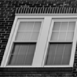
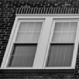

WFCA block. To evaluate the role of the proposed WFCA block, we remove the frequency module in FAM by replacing WFCA with one Conv layer and denote the model as SFANet(w/o WFCA). One can see that our model can achieve 0.2dB improvement over SFANet(w/o WFCA), which proves the effectiveness of WFCA block. By modeling deep frequency features using our WFCA block, our SFANet can reconstruct more textures (see Fig. 10).
Window-based strategy. In order to overcome the mismatch problem in the frequency domain, we propose to use the window-based strategy in WFCA. To evaluate the effectiveness of the window-based strategy, we train a variant, namely SFANet(w/o W), which performs FFT on the entire deep feature and utilizes channel attention on such frequency feature. As discussed in Sec.1, such a setting would cause the mismatch problem when inferencing images with varying size. We can see that compared with SFANet(full), the mismatch problem in SFANet(w/o W) leads to 0.06dB and 0.22dB performance degradation on Set12 and Urban100 dataset, respectively. Since the image size in urban100 (e.g., ) is very different from the training patch size (i.e., ), the mismatch problem is more obvious on urban100 dataset. SFANet(w/o W) obtains even worse results than SFANet(w/o WFCA) on Urban100 dataset.
From the visual comparison in Fig.10, we can also see that SFANet(w/o W) cannot recover more textures compared with SFANet(w/o WFCA). Similar experimental phenomena can also be found in zhang2022swinfir, i.e., the frequency module is not effective when the mismatch problem exists. To overcome the mismatch problem, our SFANet(full) utilizes the window-based strategy and can obtain significantly clearer results than SFANet(w/o WFCA) with the same number of network parameters.
Channel attention in frequency domain. To evaluate the role of the channel attention (CA) module in our model, we train two variants, i.e., without using CA module (SFANet(w/o CA)), and without performing CA on the imaginary part of frequency spectrum (SFANet(w/o IM)). We can see that by using CA on both real and imaginary parts of the frequency spectrum, SFANet(full) can obtain 0.07dB and 0.03dB improvement on Urban100 dataset than SFANet(w/o CA) and SFANet(w/o IM), respectively.
In Fig. 10, we can see that by using CA only on real part of the frequency spectrum, SFANet(w/o IM) can obtain denoising results with clearer structures and fewer artifacts than SFANet(w/o CA). By using both real and imaginary parts of the frequency spectrum, SFANet(full) can model comprehensive amplitude and phase information and obtain clearer denoising results. It is worth noting that, even without using CA in the frequency domain, SFANet(w/o CA) can also recover more textures than SFANet(w/o WFCA), which proves that modeling deep frequency feature with simple Conv layers can also improve the network ability in texture recovering.
| Set12 | Urban100 | |
| SFANet(w/o WFCA) | 31.02/0.8744 | 31.48/0.9117 |
| SFANet(w/o W) | 31.04/0.8748 | 31.45/0.9116 |
| SFANet(w/o CA) | 31.07/0.8756 | 31.60/0.9140 |
| SFANet(w/o IM) | 31.09/0.8759 | 31.64/0.9145 |
| SFANet(full) | 31.10/0.8761 | 31.67/0.9146 |
6 Conclusion
We presented a spatial-frequency attention network (SFANet) for high-performance image denoising. In particular, we proposed a window-based frequency channel attention (WFCA) module to effectively model image long-range dependency. WFCA utilized channel attention in the deep frequency feature domain. Since each frequency component contains nearly global information, WFCA can model more global dependency than traditional SA-based block with log-linear complexity. By using the window-based strategy, our WFCA solved the frequency resolution mismatch problem of previous methods and obtained 0.2dB improvement on Urban100. The channel attention mechanism was applied on both real and imaginary parts of the frequency spectrum to adaptively model comprehensive amplitude and phase information of deep frequency features. Dilated SA module was used in our SFANet to model long-term dependency in spatial domain. Our SFANet demonstrated clear advantages over existing methods in terms of PSNR/SSIM measures as well as visual quality in multiple image denoising benchmarks, especially on repetitive texture structures.
References
- (1) Eirikur Agustsson and Radu Timofte. Ntire 2017 challenge on single image super-resolution: Dataset and study. In Proceedings of the IEEE conference on computer vision and pattern recognition workshops, pages 126–135, 2017.
- (2) Saeed Anwar and Nick Barnes. Real image denoising with feature attention. In Proceedings of the IEEE International Conference on Computer Vision, pages 3155–3164, 2019.
- (3) Hanting Chen, Yunhe Wang, Tianyu Guo, Chang Xu, Yiping Deng, Zhenhua Liu, Siwei Ma, Chunjing Xu, Chao Xu, and Wen Gao. Pre-trained image processing transformer. In Proceedings of the IEEE/CVF Conference on Computer Vision and Pattern Recognition, pages 12299–12310, 2021.
- (4) Xiangyu Chen, Xintao Wang, Jiantao Zhou, and Chao Dong. Activating more pixels in image super-resolution transformer. arXiv preprint arXiv:2205.04437, 2022.
- (5) Yunpeng Chen, Haoqi Fan, Bing Xu, Zhicheng Yan, Yannis Kalantidis, Marcus Rohrbach, Shuicheng Yan, and Jiashi Feng. Drop an octave: Reducing spatial redundancy in convolutional neural networks with octave convolution. In Proceedings of the IEEE/CVF International Conference on Computer Vision, pages 3435–3444, 2019.
- (6) Mircea Cimpoi, Subhransu Maji, Iasonas Kokkinos, Sammy Mohamed, and Andrea Vedaldi. Describing textures in the wild. In Proceedings of the IEEE conference on computer vision and pattern recognition, pages 3606–3613, 2014.
- (7) Manuel Fritsche, Shuhang Gu, and Radu Timofte. Frequency separation for real-world super-resolution. In 2019 IEEE/CVF International Conference on Computer Vision Workshop (ICCVW), pages 3599–3608. IEEE, 2019.
- (8) Dario Fuoli, Luc Van Gool, and Radu Timofte. Fourier space losses for efficient perceptual image super-resolution. In Proceedings of the IEEE/CVF International Conference on Computer Vision, pages 2360–2369, 2021.
- (9) Shi Guo, Zhetong Liang, and Lei Zhang. Joint denoising and demosaicking with green channel prior for real-world burst images. IEEE Transactions on Image Processing, 30:6930–6942, 2021.
- (10) Shi Guo, Zifei Yan, Kai Zhang, Wangmeng Zuo, and Lei Zhang. Toward convolutional blind denoising of real photographs. In Proceedings of the IEEE/CVF conference on computer vision and pattern recognition, pages 1712–1722, 2019.
- (11) Jie Hu, Li Shen, and Gang Sun. Squeeze-and-excitation networks. In Proceedings of the IEEE conference on computer vision and pattern recognition, pages 7132–7141, 2018.
- (12) Yanxin Hu, Yun Liu, Shubo Lv, Mengtao Xing, Shimin Zhang, Yihui Fu, Jian Wu, Bihong Zhang, and Lei Xie. Dccrn: Deep complex convolution recurrent network for phase-aware speech enhancement. arXiv preprint arXiv:2008.00264, 2020.
- (13) Jia-Bin Huang, Abhishek Singh, and Narendra Ahuja. Single image super-resolution from transformed self-exemplars. In Proceedings of the IEEE conference on computer vision and pattern recognition, pages 5197–5206, 2015.
- (14) Xixi Jia, Sanyang Liu, Xiangchu Feng, and Lei Zhang. Focnet: A fractional optimal control network for image denoising. In Proceedings of the IEEE/CVF Conference on Computer Vision and Pattern Recognition, pages 6054–6063, 2019.
- (15) Gustaf Kylberg. The kylberg texture dataset v. 1.0. External report (Blue series) 35, Centre for Image Analysis, Swedish University of Agricultural Sciences and Uppsala University, Uppsala, Sweden, September 2011.
- (16) Svetlana Lazebnik, Cordelia Schmid, and Jean Ponce. A sparse texture representation using local affine regions. IEEE transactions on pattern analysis and machine intelligence, 27(8):1265–1278, 2005.
- (17) Junxuan Li, Shaodi You, and Antonio Robles-Kelly. A frequency domain neural network for fast image super-resolution. In 2018 International Joint Conference on Neural Networks (IJCNN), pages 1–8. IEEE, 2018.
- (18) Xin Li, Xin Jin, Tao Yu, Simeng Sun, Yingxue Pang, Zhizheng Zhang, and Zhibo Chen. Learning omni-frequency region-adaptive representations for real image super-resolution. In Proceedings of the AAAI Conference on Artificial Intelligence, volume 35, pages 1975–1983, 2021.
- (19) Jingyun Liang, Jiezhang Cao, Guolei Sun, Kai Zhang, Luc Van Gool, and Radu Timofte. Swinir: Image restoration using swin transformer. In Proceedings of the IEEE/CVF International Conference on Computer Vision, pages 1833–1844, 2021.
- (20) Bee Lim, Sanghyun Son, Heewon Kim, Seungjun Nah, and Kyoung Mu Lee. Enhanced deep residual networks for single image super-resolution. In Proceedings of the IEEE conference on computer vision and pattern recognition workshops, pages 136–144, 2017.
- (21) Ding Liu, Bihan Wen, Yuchen Fan, Chen Change Loy, and Thomas S Huang. Non-local recurrent network for image restoration. Advances in neural information processing systems, 31, 2018.
- (22) Pengju Liu, Hongzhi Zhang, Kai Zhang, Liang Lin, and Wangmeng Zuo. Multi-level wavelet-cnn for image restoration. In Proceedings of the IEEE conference on computer vision and pattern recognition workshops, pages 773–782, 2018.
- (23) Kede Ma, Zhengfang Duanmu, Qingbo Wu, Zhou Wang, Hongwei Yong, Hongliang Li, and Lei Zhang. Waterloo exploration database: New challenges for image quality assessment models. IEEE Transactions on Image Processing, 26(2):1004–1016, 2016.
- (24) David Martin, Charless Fowlkes, Doron Tal, and Jitendra Malik. A database of human segmented natural images and its application to evaluating segmentation algorithms and measuring ecological statistics. In Proceedings Eighth IEEE International Conference on Computer Vision. ICCV 2001, volume 2, pages 416–423. IEEE, 2001.
- (25) Chong Mou, Jian Zhang, and Zhuoyuan Wu. Dynamic attentive graph learning for image restoration. In Proceedings of the IEEE/CVF International Conference on Computer Vision, pages 4328–4337, 2021.
- (26) Yingxue Pang, Xin Li, Xin Jin, Yaojun Wu, Jianzhao Liu, Sen Liu, and Zhibo Chen. Fan: Frequency aggregation network for real image super-resolution. In European Conference on Computer Vision, pages 468–483. Springer, 2020.
- (27) Tobias Plötz and Stefan Roth. Neural nearest neighbors networks. Advances in Neural information processing systems, 31, 2018.
- (28) Ying Tai, Jian Yang, Xiaoming Liu, and Chunyan Xu. Memnet: A persistent memory network for image restoration. In Proceedings of the IEEE international conference on computer vision, pages 4539–4547, 2017.
- (29) Zhengzhong Tu, Hossein Talebi, Han Zhang, Feng Yang, Peyman Milanfar, Alan Bovik, and Yinxiao Li. Maxim: Multi-axis mlp for image processing. arXiv preprint arXiv:2201.02973, 2022.
- (30) Diego Valsesia, Giulia Fracastoro, and Enrico Magli. Deep graph-convolutional image denoising. IEEE Transactions on Image Processing, 29:8226–8237, 2020.
- (31) Xintao Wang, Ke Yu, Chao Dong, and Chen Change Loy. Recovering realistic texture in image super-resolution by deep spatial feature transform. In The IEEE Conference on Computer Vision and Pattern Recognition (CVPR), June 2018.
- (32) Zhihao Xia, Federico Perazzi, Michaël Gharbi, Kalyan Sunkavalli, and Ayan Chakrabarti. Basis prediction networks for effective burst denoising with large kernels. In Proceedings of the IEEE/CVF Conference on Computer Vision and Pattern Recognition, pages 11844–11853, 2020.
- (33) Wenbin Xie, Dehua Song, Chang Xu, Chunjing Xu, Hui Zhang, and Yunhe Wang. Learning frequency-aware dynamic network for efficient super-resolution. In Proceedings of the IEEE/CVF International Conference on Computer Vision, pages 4308–4317, 2021.
- (34) Syed Waqas Zamir, Aditya Arora, Salman Khan, Munawar Hayat, Fahad Shahbaz Khan, and Ming-Hsuan Yang. Restormer: Efficient transformer for high-resolution image restoration. In Proceedings of the IEEE/CVF Conference on Computer Vision and Pattern Recognition, pages 5728–5739, 2022.
- (35) Syed Waqas Zamir, Aditya Arora, Salman Khan, Munawar Hayat, Fahad Shahbaz Khan, Ming-Hsuan Yang, and Ling Shao. Learning enriched features for real image restoration and enhancement. arXiv preprint arXiv:2003.06792, 2020.
- (36) Dafeng Zhang, Feiyu Huang, Shizhuo Liu, Xiaobing Wang, and Zhezhu Jin. Swinfir: Revisiting the swinir with fast fourier convolution and improved training for image super-resolution. arXiv preprint arXiv:2208.11247, 2022.
- (37) Kai Zhang, Yawei Li, Wangmeng Zuo, Lei Zhang, Luc Van Gool, and Radu Timofte. Plug-and-play image restoration with deep denoiser prior. IEEE Transactions on Pattern Analysis and Machine Intelligence, 2021.
- (38) Kai Zhang, Wangmeng Zuo, Yunjin Chen, Deyu Meng, and Lei Zhang. Beyond a gaussian denoiser: Residual learning of deep cnn for image denoising. IEEE Transactions on Image Processing, 26(7):3142–3155, 2017.
- (39) Kai Zhang, Wangmeng Zuo, Shuhang Gu, and Lei Zhang. Learning deep cnn denoiser prior for image restoration. In Proceedings of the IEEE conference on computer vision and pattern recognition, pages 3929–3938, 2017.
- (40) Kai Zhang, Wangmeng Zuo, and Lei Zhang. Ffdnet: Toward a fast and flexible solution for cnn-based image denoising. IEEE Transactions on Image Processing, 27(9):4608–4622, 2018.
- (41) Xindong Zhang, Hui Zeng, Shi Guo, and Lei Zhang. Efficient long-range attention network for image super-resolution. arXiv preprint arXiv:2203.06697, 2022.
- (42) Long Zhao, Zizhao Zhang, Ting Chen, Dimitris Metaxas, and Han Zhang. Improved transformer for high-resolution gans. Advances in Neural Information Processing Systems, 34, 2021.
- (43) Shengkui Zhao, Bin Ma, Karn N Watcharasupat, and Woon-Seng Gan. Frcrn: Boosting feature representation using frequency recurrence for monaural speech enhancement. In ICASSP 2022-2022 IEEE International Conference on Acoustics, Speech and Signal Processing (ICASSP), pages 9281–9285. IEEE, 2022.