\@openrightfalse{committee}\advisor

Dr.AlessandroGiusti \coadvisorDr.JèrômeGuzzi \Day16 \MonthOctober \Year2020 \placeLugano \dedicationTo everyone who taught me something \openepigraph“It has become appallingly obvious that our technology has exceeded our humanity.”Albert Einstein

Simulation of robot swarms for learning
communication-aware coordination

Giorgia Adorni

Abstract

In recent years, robotics research has dedicated extensive attention to cooperative multi-agent problems, in which agents have a common goal that requires them to collaborate and possibly communicate, to achieve it. We investigate imitation learning algorithms to address this issue, providing new insights and promising solutions. These methods learn a controller by observing demonstrations of an expert, such as the behaviour of a centralised omniscient controller, which can perceive the entire environment, including the state and observations of all agents.

Performing tasks with complete knowledge of the state of a system is relatively easy, but centralised solutions might not be feasible in real scenarios since agents do not have direct access to the state but only to their own observations. To overcome this issue, we train end-to-end Neural Networks, usually classifiers or regressors, that take as input local observations obtained from an omniscient centralised controller, in other words, the agents’ sensor readings and the communications received, producing as output the action to be performed and the communication to be transmitted.

In this study, we focus on two different scenarios: distributing the robots in space such that they stand at an equal distance from each other and colouring the robots in space depending on their position with respect to the others in the group. Both are examples of cooperative tasks based on the use of a distributed controller. While the second cannot be solved without allowing an explicit exchange of messages between the agents, in the first one, a communication protocol is unnecessary, although it may increase performance.

The experiments are run in Enki, a high-performance open-source simulator for planar robots, which provides collision detection and limited physics support for robots evolving on a flat surface. Moreover, it can simulate groups of robots hundreds of times faster than real-time.

The results show how applying a communication strategy improves the performance of the distributed model, letting it decide which actions to take almost as precisely and quickly as the expert controller.

Acknowledgements.

I would like to thank my supervisors Alessandro Giusti and Jérôme Guzzi for their precious advice and help, my family who have never stopped believing in me and to Elia who shared with me this extraordinary journey, always encouraging and supporting me, despite all the difficulties. A special thank goes also to Università della Svizzera Italiana and the University of Milano–Bicocca for allowing me to take part in this double degree program and to all those people who have accompanied me and made this experience special.

Contents

chapter*.2chapter*.2chapter*.3chapter*.4chapter*.5chapter.1chapter.2section.2.1subsection.2.1.1subsection.2.1.2subsubsection.2.1.2.1subsubsection.2.1.2.2section.2.2subsection.2.2.1subsection.2.2.2subsection.2.2.3chapter.3section.3.1subsection.3.1.1subsection.3.1.2subsection.3.1.3subsection.3.1.4section.3.2subsection.3.2.1subsection.3.2.2section.3.3chapter.4section.4.1section.4.2section.4.3subsection.4.3.1subsection.4.3.2section.4.4section.4.5subsection.4.5.1subsubsection.4.5.1.1subsubsection.4.5.1.2subsection.4.5.2subsubsection.4.5.2.1subsubsection.4.5.2.2subsection.4.5.3subsubsection.4.5.3.1subsubsection.4.5.3.2subsubsection.4.5.3.3chapter.5section.5.1subsection.5.1.1subsubsection.5.1.1.1subsubsection.5.1.1.2subsubsection.5.1.1.3subsubsection.5.1.1.4subsection.5.1.2subsubsection.5.1.2.1subsubsection.5.1.2.2subsubsection.5.1.2.3subsubsection.5.1.2.4section.5.2subsection.5.2.1subsubsection.5.2.1.1subsubsection.5.2.1.2subsubsection.5.2.1.3chapter.6chapter.6section.6.1section.6.2appendix.Asection*.183

List of Figures

figure.caption.6figure.caption.7 figure.caption.9figure.caption.10figure.caption.11figure.caption.12figure.caption.15 figure.caption.19figure.caption.22 figure.caption.28figure.caption.29figure.caption.30figure.caption.31figure.caption.32figure.caption.33 figure.caption.35figure.caption.37figure.caption.38figure.caption.39figure.caption.40figure.caption.41figure.caption.42figure.caption.43figure.caption.44figure.caption.46figure.caption.47figure.caption.48figure.caption.49figure.caption.51figure.caption.52figure.caption.53figure.caption.54figure.caption.56figure.caption.57figure.caption.58figure.caption.59figure.caption.60figure.caption.62figure.caption.63figure.caption.64figure.caption.66figure.caption.68figure.caption.70figure.caption.71figure.caption.72figure.caption.73figure.caption.74figure.caption.75figure.caption.76figure.caption.78figure.caption.79figure.caption.80figure.caption.81figure.caption.82figure.caption.83figure.caption.84figure.caption.86figure.caption.87figure.caption.88figure.caption.89figure.caption.90figure.caption.91figure.caption.92figure.caption.94figure.caption.95figure.caption.97figure.caption.99figure.caption.100figure.caption.101figure.caption.102figure.caption.104figure.caption.106figure.caption.107figure.caption.108figure.caption.110figure.caption.111figure.caption.112figure.caption.113figure.caption.115figure.caption.117figure.caption.118figure.caption.119figure.caption.121figure.caption.122figure.caption.123figure.caption.124figure.caption.126figure.caption.127figure.caption.128figure.caption.129figure.caption.131figure.caption.132figure.caption.134figure.caption.136figure.caption.137figure.caption.138figure.caption.139figure.caption.140figure.caption.141figure.caption.142figure.caption.144figure.caption.145figure.caption.146figure.caption.147figure.caption.148figure.caption.149figure.caption.150figure.caption.152figure.caption.153figure.caption.154figure.caption.155figure.caption.156figure.caption.158figure.caption.159figure.caption.160figure.caption.162figure.caption.164figure.caption.165figure.caption.166figure.caption.167figure.caption.169figure.caption.170figure.caption.171figure.caption.172figure.caption.174figure.caption.175figure.caption.176figure.caption.177figure.caption.178figure.caption.180figure.caption.181

List of Tables

figure.caption.34figure.caption.67figure.caption.96figure.caption.133figure.caption.161

\@mainmattertrue

Introduction

In this work, we consider cooperative multi-agent scenarios, in which multiple robots collaborate and possibly communicate to achieve a common goal Ismail and Sariff 2018. Homogeneous Multi-Agent Systems (MAS) are composed of $N$ interacting agents, which have the same physical structure and observation capabilities, so they can be considered to be interchangeable and cooperate to solve a given task Stone and Veloso 2000; Šošić et al. 2016. This system is characterised by a state $S$ — which can be decomposed into sets of local states for each agent and the set of possible observations $O$ for each agent — obtained through sensors and the set of possible actions $A$ for each agent.

The objective of this study is to use Imitation Learning approaches to learn decentralised solutions via imitation of an omniscient centralised control. To do so, we train end-to-end Neural Networks, either classifiers or regressors, that only exploit local observations and communications to decide the action to be performed. This controller is the same for each agent, which means that given an identical set of observations as input, likewise, for each of these, the outputs will be equivalent Ross et al. 2011; Tolstaya et al. 2020.

This research project focuses on two different multi-agent scenarios, in which $N$ robots, all oriented in the same direction, are initially randomly placed along the $x$ -axis. We consider the Thymio as holonomic since their movements are limited to only one dimension. This premise simplifies our system, in which consequently we have to keep into account only geometric constraints and not kinematic ones.

In the first scenario, visualised in Figure 1, the objective is to distribute the robots in space such that they stand at equal distances from each other. To do so, each agent updates its state — its absolute position — by performing actions — moving forward and backwards along the $x$ -axis — based on the observations received from the environment — the distances from neighbours.

Refer to caption — Figure 1: Visualisation of the initial and final configurations obtained simulating the first task.

Perceiving the environment using its own sensors, in particular sensing the distances from the neighbours, each robot achieves the goal moving towards the target by minimising the difference between the values recorded by the front and rear sensors, trying to maintain the maximum achievable speed. This means that each robot is at the same distance from the one in front and the one behind, that should be the same distance among all the agents.

In the second scenario, shown in Figure 2, assuming that the agents in space are divided into two sets, the objective is to colour them depending on their group membership. For the sake of simplicity, we decide the group each robot belongs to based on the total number of robots: in case of an even number of agents, those in the first half of the row belong to the first group and the remaining to the second, while in the case of an odd number of robots, the same reasoning is applied and the central agent is assigned to the first set. To perform this task, each agent performs actions — colouring the top Light Emitting Diode in red or blue — based on the observations received from the environment — the messages received from neighbours.

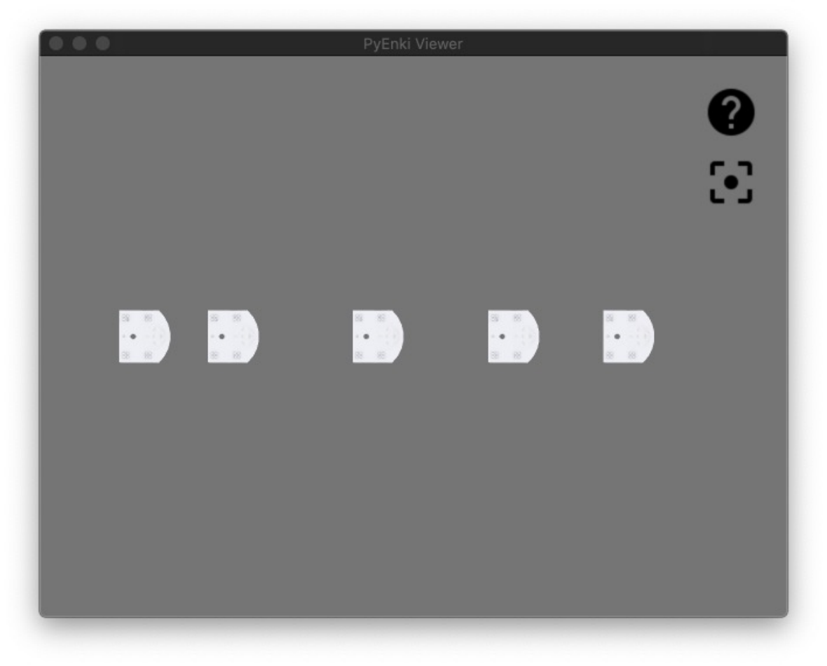
This time, sensing the distance from neighbours does not provide useful information about the order of the agents, therefore they are not considered to accomplish this task. Instead, the only way for the robots to understand their ordering is necessarily using a communication protocol. For example, starting from the extreme agents, the first and the last in the row, or those that cannot receive any communication respectively from back and front, all the robots retransmit the received value, increased by one. In this way, the agents will in a sense, learn to count in order to understand which is the correct value to transmit.

Both the scenarios are examples of cooperative tasks based on the use of a distributed controller. While the second cannot be solved without allowing an explicit exchange of messages between the agents, in the first one a communication protocol is not necessary, but it may nonetheless increase performance. To solve these tasks we have adopted two different methodologies, depending on whether the communication is used or not. First of all, we analyse typical supervised learning approaches, which directly learn a mapping from observations to actions. This method can be applied only to the first task, in which a very simple “distributed network” that takes as input an array containing the response values of the sensors — either prox_values, prox_comm or all_sensors — and produces as output an array containing one float that represents the speed of the wheels, which is assumed to be the same both right and left, so that the robot moves straight. After that, we concentrate on more challenging situations where the communication is not provided to the network, instead, it is a latent variable which has to be inferred Le et al. 2017. Throughout the experiments, we show the effectiveness of our methods, comparing approaches with and without communication. We also analyse the effects of varying the inputs of the networks, the initial distance between the robot and the number of agents chosen.

Outline

The thesis is composed of 6 chapters, whose main points are presented as follows:

•

Chapter Literature review summarises the previous research on the topic, evaluating the approaches adopted by the authors;
•

Chapter Background provides the background knowledge needed to properly understand the research contents;
•

Chapter Tools presents the tools used for the data collection and all the additional frameworks we relied on;
•

Chapter Methodologies thoroughly illustrates the methodology used, their benefits and limitations, also including descriptions of the kind of data used and how they are collected;
•

Chapter Evaluation explores the analysis conducted and shows evaluation results;
•

The Conclusion addresses the results of the experiments, concludes the thesis by discussing the implications of our findings, possible improvements and outlines future works.

Literature review

This chapter discusses previous research about the topic, providing a brief introduction to the approach we adopted.

In recent years, the application of Artificial Intelligence and Deep Learning techniques to multi-agent cooperative problems has become increasingly successful. Gasser and Huhns, in Distributed Artificial Intelligence Gasser and Huhns 2014, have addressed the issue of coordination and cooperation among agents with the combination of distributed systems and Artificial Intelligence, a discipline known as Distributed Artificial Intelligence.

Similarly, Panait and Luke, in their work Cooperative multi-agent learning: The state of the art Panait and Luke 2005, report that Multi-Agent Learning, the application of machine learning to problems involving multiple agents, has become a popular approach which deals with unusually large search spaces. In addition, they mention three of the most classic techniques used to solve cooperative Multi-Agent problems, that are Supervised and Unsupervised Learning, and Reinforcement Learning. These methods are distinguished according to the type of feedback provided to the agent: the target output in the first case, no feedback is provided in the second, and reward based on the learned output in the last one.

Given these three options, the vast majority of articles in this field used reward-based methods to approach Multi-Agent Learning scenarios, in particular Reinforcement Learning, that make they possible to achieve sophisticated goals in complex and uncertain environments Oliehoek 2012. However, this technique is notoriously known for being hard, in particular it is difficult to design a suitable reward function for the agents to optimise, which precisely leads to the desired behaviour in all possible scenarios. This problem is further exacerbated in multi-agent settings Hadfield-Menell et al. 2017; Oliehoek 2012.

Inverse Reinforcement Learning addresses this problem by using a given set of expert trajectories to derive a reward function under which these are optimal. Nevertheless, this technique imposes often unrealistic requirements Šošić et al. 2016.

Imitation Learning is a class of methods that has been successfully applied to a wide range of domains in robotics, for example, autonomous driving Schaal 1999; Stepputtis et al. 2019. They aim to overcome the issues aforementioned and, unlike reward-based methods, the model acquires skills and provides actions to the agents by observing the desired behaviour, performed by an expert Song et al. 2018; Zhang et al. 2018; Billard et al. 2008. Using this approach the models learn how to extract relevant information from the data provided to them, directly learning a mapping from observations to actions. A more challenging situation occurs when the model also has to infer the coordination among agents that is implicit in the demonstrations, using unsupervised approaches to imitation.

In this direction, literature suggests that cooperative tasks sometimes cannot be solved using only a simple distributed approach, instead it may be necessary to allow an explicit exchange of messages between the agents. In Multi-agent reinforcement learning: Independent vs. cooperative agents Tan 1993, Tan affirms that cooperating learners should use communication in a variety of ways in order to improve team performance: they can share instantaneous informations as well as episodic experience and learned knowledge. Also Pesce and Montana propose the use of inter-agent communication for situations in which the agents can only acquire partial observations and are faced with a task requiring coordination and synchronisation skills Pesce and Montana 2019. Their solution consists in an explicit communication system that allows agents to exchange messages that are used together with local observations to decide which actions to take.

Our work is based on Learning distributed controllers by backpropagation Verna 2020, which proposes an approach in which a distributed policy for the agents and a coordination model are learned at the same time. This method is based on an important concept introduced in Coordinated multi-agent imitation learning Le et al. 2017: the network has the ability to autonomously determine the communication protocol. Likewise, we use imitation learning approaches to solve the problem of coordinating multiple agents, introducing a communication protocol, which consists in an explicit exchange of messages between the robots. The communication is not provided to the network, instead, it is a latent variable which has to be inferred. The results show the effectiveness of this communication strategy developed, as well as an illustration of the different patterns emerging from the tasks.

Background

This chapter provides some background concepts to understand the material presented in this thesis. We start Section Differential drive robots with a review about differential drive robots and their kinematics, providing some useful notions about the types of sensors used and finally summarising the theory of control. We conclude with a refresher on Neural Networks, in Section Artificial Neural Networks.

Differential drive robots

The robot we use for this study is Thymio II, a non-holonomic differential drive robot.

A differential wheeled vehicle is mobile robot, that typically consists of a rigid body

and a mobile base with a system of wheels that allows movement in the environment. Its movements are based on two, independently powered and controlled, fixed wheels, placed on either side of the robot body, with a common axis of rotation, and one passive caster wheel, whose job is to keep the robot statically balanced. Thus, both drive and steering functions are provided. In fact, it is possible to impose different values of velocity for the two fixed wheels, allowing the robot to rotate and move back and forth Siciliano et al. 2010. It is important to note that the robot is non-holonomic since it cannot translate laterally.

The Instantaneous Center of Curvature, is the point which lies along the horizontal axis, common to the left and right wheels, perpendicular to the plane of each wheel. Its position changes over time as a function of the individual wheel velocities, in particular of their relative difference. Since the rate of rotation $\omega$ is the same for both wheels, the following expressions hold:

\omega\,(R+b)=V_{rx}

(1)

\omega\,(R-b)=V_{lx}

(2)

Equation 0.1: Right and left linear velocities of a differential drive robot, computed as function of the rotation rate, the distance between the wheels, and the distance from the Instantaneous Center of Curvature and the robot reference point.

where $b$ is the distance between the centres of the two wheels, $V_{rx}$ and $V_{lx}$ are the right and left wheel velocities, and $R$ is the signed distance from the Instantaneous Center of Curvature to the midpoint between the wheels $P_{O}$ Dudek and Jenkin 2010. Moreover, at any specific time instant $t$ we can compute $R$ and $\omega$ as follows:

R=b\,\frac{V_{rx}+V_{lx}}{V_{rx}-V_{lx}}

(3)

Equation 0.2: Function to compute

R

, the signed distance from the Instantaneous Center of Curvature to the midpoint between the wheels

P_{O}

, or robot reference point, using the right and left linear velocities and the distance between the centres of the two wheels.

\omega=\frac{V_{rx}-V_{lx}}{2b}

(4)

Equation 0.3: Function to compute

\omega

, the angular velocity of the robot, using the right and left linear velocities and the distance between the centres of the two wheels.

As a consequence, by varying the speed of the two wheels, $V_{rx}$ and $V_{lx}$ , the trajectories that the robot takes changes as well:

•

$V_{rx}=V_{lx}$ : if the same speed is set to both wheels, we have a forward linear motion in a straight line. $R$ becomes infinite, and there is effectively no rotation $\omega=0$ .
•

$V_{rx}=-V_{lx}$ : if both wheels are driven with equal speed but in the opposite direction, we have a rotation about the midpoint of the wheel axis, or in-place rotation. $R=0$ , the Instantaneous Center of Curvature coincide with $P_{O}$ and $\omega=-\frac{V}{b}$ .
•

$V_{lx}=0$ : if the left wheel is not powered, we have a counter-clockwise rotation about the left wheel. $R=b$ and $\omega=\frac{V_{rx}}{2b}$ .
•

$V_{rx}=0$ : if the right wheel is not powered, we have a clockwise rotation about the right wheel. $R=-b$ and $\omega=-\frac{V_{lx}}{2b}$ .

Differential drive robots, however, are sensitive to slight changes in velocity, and even small errors can affect the robot trajectory. Moreover, they are also susceptible to variations in the ground.

Sensors

A significant feature of the Thymio II robot, is the a large number of sensors with which it is equipped.

The adoption of external sensing mechanism is of crucial importance to allow a robot to interact with its environment and achieve high-performance Fu et al. 1987; Siciliano et al. 2010.

It is possible to classify the sensors in two principal categories, according to their function: proprioceptive sensors, that measure the internal state and deal with the the detection of variables used for the control, such as the robot position, and exteroceptive sensors that measure the external state of the environment, dealing with the detection of variables such as range and proximity, often used for robot guidance as well as object detection.

For the purposes of this thesis we are interested in the study of proximity sensors, in particular the Infrared sensors, that used by Thymio II.

Proximity sensors are an example of exteroceptive sensors: they gather information from the environment around the robot, such as distance to objects. They are also active sensors: they emit their own energy, usually light, and measure the reflection. Among the advantages of this type of sensors is the fact that the infrared beams generated by the sources can be used unobtrusively, since they are invisible to the human eye.

Infrared sensors are composed of an emitter, which radiates invisible infrared light, and a receiver, that measures the intensity of the reflection and the quantity of light that comes back. If the reflection is strong enough — a large part of the light is reflected from the object and returns to the robot — it can be inferred that the obstacle is relatively close and lies within a certain range of the sensor, depending on the received intensity. If the object is farther away, only a small part of the light comes back Fu et al. 1987. However, this estimate can be significantly affected by some property of the obstacle, such as its colour and reflectivity, but also by the presence of external light sources and the temperature of the environment — e.g. a black object reflects less light than a white one, placed at the same distance Ben-Ari and Mondada 2018.

Control theory

The problem of controlling a robot is of a primary importance: to achieve a given task, an agent must acts based on the perception received from the environment. To do so, robots use a controller that takes decisions according to algorithms developed to accomplish the goal.

We can distinguish two main techniques of control: open-loop control sets in advance the parameters of the algorithm and never observes the result of its actions to adjust them to the actual state, closed-loop control or feedback-based control, measures the error between the desired state of the system and the actual one, and uses this feedback to to adjust the control and decide the next action to take Ben-Ari and Mondada 2018.

These methods can be used to compute trajectories that lead the robot from an initial configuration to a final one. To achieve a more appropriate behaviour we are interested in the use of closed-loop control systems Siegwart et al. 2011.

Figure 4: Closed-loop control system.

This model can be formally defined using the variables introduced below:

•

$x(t)$ , called command or set point (SP), represents the reference value, or a desired output. It cannot be imposed directly on the robot, instead it is transformed into a control value $u(t)$ .
•

$u(t)$ , called control variable, is the output of the control and the input of the robot.
•

$y(t)$ , called process variable (PV), represents an observable part of the the actual state of the robot. It is the feedback signal combined with the set point to compute the error value.
•

$e(t)$ is the error. It is computed as the difference between the value of the set point and the process variable, as shown in Equation 0.4. The error is used to generate the new control signal $u(t)$ .

$e(t)=x(t)-y(t)$ (5)

Equation 0.4: Calculation of the error value $e(t)$ of the system.

The closed-loop control algorithms sometimes can be very sophisticated. For the purpose of this study, we design two algorithms, the first one is a Proportional Integral Derivative controller, while the second a Bang Bang controller.

The implementation of any feedback controller requires the availability of the robot configuration at each time instant.

Proportional (P) controller

Considering real situations in which agents do not have access to their states but only to their local observations, the controller we design for achieve the goal of the first task is a Proportional (P) Controller, a particular variant of Proportional Integral Derivative Controller, with only the $K_{p}$ term, more details are provided in the Section Task 1: Distributing the robots in space.

The closed-loop control uses a feedback to adjust the control while the action takes place in proportion to the existing error. This function, given a desired output $x(t)$ , or set point, produces an output $y(t)$ , or process variable, such that the error $e(t)$ is obtained as the difference between the value of the set point and the process variable. Finally, the control variable $u(t)$ is the output of the Proportional Integral Derivative controller and is computed as follows:

u(t)=K_{p}*e(t)

(6)

Equation 0.5: Proportional Proportional Integral Derivative controller.

The value of the proportional gain can be tuned to yield satisfactory performance so that the system is stable.

Bang-bang controller

The controller we design to achieve the goal of the first task, of which more details are provided in the Section Task 1: Distributing the robots in space, is a variant of the Bang-bang algorithm.

In this case we considered instead a situation in which agents have access to their states: given the set point and the variable measured, the goal and the actual position of the robot, the error is computed as the difference between the two quantities. What we want to achieve is that the error is 0, to do so, when the error is negative, the robot should move forward to reach the goal, on the contrary if is positive it should move backwards. Its main feature is that the motor powers are turned to full forwards or full backwards depending on the sign of the error.

This approach has many advantages, such as its simplicity and no need for calibration. However, since this controller is not always precise, especially when a derivative term is needed to avoid oscillations or when we are in steady-state, close to desired value, we implemented a variant that moves the the robot at full speed unless they are closer than a certain value, avoiding to approach the goal at full speed and overshoot it.

Artificial Neural Networks

In the field of Machine Learning, Artificial Neural Networks are mathematical models based on the simplification of Biological Neural Networks Zou et al. 2008.

A Neural Network can be considered as a dynamic system having the topology of an oriented graph, whose nodes model the neurons in a biological brain, while the edges represent the synapses — interconnections of information. Each connection can transmit a signal from one artificial neuron to another, which are typically aggregated in layers. The stimuli are received by a level of input nodes, called processing unit, which processes the signal and transmits it to other neurons connected to it.

As we anticipated, Neural Networks can be seen as mathematical models that define a function $f:X\rightarrow Y$ . The network function of a neuron $f(x)$ is defined as a composition of other functions $g_{i}(x)$ , which can in turn be decomposed into others. A widely used representation for the description of traditional Artificial Neural Networks is the weighted sum, shown in Equation 0.6.

f(x)=\phi\bigg(\sum_{i}w_{i}x_{i}+\theta\bigg)

(7)

Equation 0.6: Function that describes mathematically the traditional Artificial Neural Networks in terms of weighted sum.

Each input signal $x_{i}$ is multiplied by its corresponding weight $w_{i}$ , which assumes a positive or negative value depending on whether you want to excite or inhibit the neuron. The bias $\theta$ varies according to the propensity of the neuron to activate, influencing its output. Additionally, a predefined function $\phi$ can be applied, also called activation function, which is explained in the following paragraph.

Activation functions

An activation function is a fundamental component of the model. It allows the network to learn non-linear transformations, in order to be able to compute non-trivial problems. In the course of this study, we used two of the most popular activation functions in deep learning, the hyperbolic tangent (Tanh) Kalman and Kwasny 1992 and the sigmoid Han and Moraga 1995, visualised in Figure 7.

Tanh

The tanh is a zero-centred function, whose range lies between $(-1,1)$ , and its output is given by the following formula:

f(x)=\frac{\sinh(x)}{\cosh(x)}=\bigg(\frac{e^{x}-e^{-x}}{e^{x}+e^{-x}}\bigg)

(8)

Equation 0.7: Hyperbolic Tangent Function (Tanh).

Sigmoid

The sigmoid models the frequency of the stimuli emitted by an inactive neuron, $\sigma(x)=0$ , to one fully saturated with the maximum activation frequency, $\sigma(x)=1$ . Its output is given by the following formula:

\sigma(x)=\frac{1}{1+e^{-x}}

(9)

Equation 0.8: Sigmoid Function.

(a) Tanh activation function.

(b) Sigmoid activation function.

Figure 7: Trends of two non-linear activation functions.

Loss functions

The learning process is structured as a non-convex optimisation problem in which the aim is to minimise a cost function, which measures the distance between a particular solution and an optimal one.

In the course of this study we used two different objective functions, depending on the strategy to be adopted: to solve the first task, that can be modelled as a regression problem, we used the Mean Squared Error Wang and Bovik 2009, while for the second, that is a binary classification problem, we used the Binary Cross Entropy Gómez 2018.

Mean Squared Error

The Mean Squared Error computes the deviation between the values observed $\hat{y}_{i}$ and those predicted by the network $y_{i}$ , over the number of predictions $n$ , as shown in Equation 0.9.

\mathtt{MSE}=\frac{\sum_{i=1}^{n}(y_{i}-\hat{y}_{i})^{2}}{n}

(10)

Equation 0.9: Mean Squared Error (MSE) loss function.

Formally, this criterion measures the average of squared error between predictions and targets, and learns to reduce it by penalising big errors in the model predictions.

Binary Cross Entropy

The Binary Cross Entropy is a combination of the sigmoid activation and the Cross Entropy. It sets up a binary classification problem between two classes, with the following formulation:

\mathtt{BCE}=-\frac{1}{n}\sum_{i=1}^{n}y_{i}\cdot\log(\hat{y}_{i})+(1-y_{i})\cdot\log(1-\hat{y}_{i})

(11)

Equation 0.10: Binary Cross Entropy (Binary Cross Entropy) loss function Sadowski 2016.

where $\hat{y}_{i}$ is the $i$ -th scalar value in the model output, $y_{i}$ is the corresponding target value, and $n$ is the number of scalar value in the model output¹¹ 1 https://peltarion.com/knowledge-center/documentation/modeling-view/build-an-ai-model/loss-functions/binary-crossentropy.

This loss function should return high values for bad predictions and low values for good ones.

Optimisation algorithms

Optimisation algorithms are needed to minimise the result of a given objective function, which depends on the parameters the model has to learn during training. They strongly influence the effectiveness of the learning process as they update and calculate the appropriate and optimal values of that model. In particular, the extent of the update is determined by the learning rate, which guarantees convergence to the global minimum, for convex error surfaces, and to a local minimum, for non-convex surfaces.

Adam

The optimiser we have chosen for this thesis project is Adam, an algorithm for first-order gradient-based optimisation of stochastic objective functions, based on adaptive estimates of lower-order moments Kingma and Ba 2014; Loshchilov and Hutter 2017.

Tools

This chapter introduces the tools used in this work, starting from the description of the target platform in Section Thymio II, then describing the simulator in Section Enki simulator and finally mentioning the frameworks used for the implementation in Section Frameworks.

Thymio II

The target platform is Thymio II, a small differential drive mobile robot developed in the context of a collaboration between the MOBOTS group of the Swiss Federal Institute of Technology in Lausanne and the Lausanne Arts School.

Thymio runs the Aseba open-source programming environment, an event-based modular architecture for distributed control of mobile robots, designed to enable beginners to program easily and efficiently Magnenat et al. 2010; Mondada et al. 2017, making it well-suited for robotic education and research.

Another particularity of this tool is the integration with the open-source Robot Operating System Quigley et al. 2009, through asebaros bridge Magnenat 2010.

The Thymio II includes sensors that can measure light, sound and distance. It can perform actions such as move using two wheels, each powered by its own motor, but also turning lights on and off.

Motors

The robot is equipped with two motors, each connected to one of the two wheels, which allow the robot to move forward, backwards but also turn by setting the velocity of the wheels at different speeds. The maximum speed allowed to the agent is $16.6$ cm/s.

Sensors

Thymio II possesses a large number of sensors, but for the purpose of this study we focused only on usage of the horizontal proximity ones.

Around the robot periphery are positioned $7$ distances sensors, five on the front and two on the rear. These sensors can measure the distances to nearby objects thanks to the use of Infrared, addressed in Section Sensors.

Communication

Thymio II can employ its horizontal Infrared sensors to communicate a value to robots within a range of about $48$ cm. In particular, the robot can enable the proximity communication and send an integer payload of $11$ bits at $10$ Hz, one value transmitted every $0.1$ s. This message is received by other agents if at least one of their proximity sensors is visible by one of the emitter’s Light Emitting Diodes and if they have enabled the proximity communication. Every time that a message is received by some robot, an event is created containing the message, payload data and intensities data.

LEDs

Thymio II holds many Light Emitting Diodes scattered around its body, most of them are associated with sensors and can highlight their activations.

In this study, specifically for the objectives of Task 2 introduced later in Section Task 2: Colouring the robots in space, two Red Green Blue Light Emitting Diodes on the top of the robot are used and driven together. It is possible to set the intensities of the top Light Emitting Diodes, in particular choosing the value for each channel (red, green and blue) in a range from $0$ (off) to $32$ (fully lit).

Enki simulator

Enki is the open-source robot simulator used in this project. It provides collision and limited physics support for robots evolving on a flat surface and can simulate groups of robots a hundred times faster than real-time Magnenat et al. 1999.

In this project, we exploit the PyEnki package Guzzi 2020 that provides Python bindings to the Enki simulator using Boost::Python Seefeld 2002-2015. Moreover, it adds some functionalities to the original simulator such as the support for the proximity communication between Thymio II. Another peculiarity is that the simulated world can be run in real time inside a Qt application or even without the Graphical User Interface as fast as possible.

In the simulator, the environment is represented as a three-dimensional Cartesian coordinate system, defined by three pair-wise perpendicular axes, $x$ , $y$ and $z$ , that go through the origin in $(0,0,0)$ .

In the following sections, the functioning of motors and sensors are explored in detail, as well as the concept of communication, anticipated in Section Communication, giving particular attention to the explanation of their use in the simulator.

Motors

As for the motors, they are used to establish the speed of the wheels. The target wheels’ speed can be set by writing the variables motor_{left,right}_target. The velocity is a float value specified in centimetres per second (cm/s). The wheels at maximum maximum allowed speed can provide a velocity of $16.6$ cm/s.

Another important element used for the construction of the model constraints is the distances between the left and right driving wheels, that is fixed to $9.4$ cm.

Finally, a little amount of relative noise, about $0.027$ , is added to the target wheel speed at each control step.

Sensors

In Enki, it is possible to access the Thymio sensor readings in two different ways, by using prox_values and prox_comm_events.

prox_values

an array of floats that holds the values of $7$ horizontal distance sensors around its periphery [fll (front left left), fll (front left), fc (front centre), fr (front right right), frr (front right), bl (back left), br (back right)]. These values can vary from $0$ — when the robot does not see anything — up to $4505$ — when the robot is very close to an obstacle. Thymio II updates this array at a frequency of $10$ Hz, generating the prox event after every update. The maximum range of these sensors is $14$ cm.

prox_comm_events

a list of events, one for every received message collected during the last control step of the simulation. After enabling the proximity communication, using prox_comm_enable command, the robot can use the horizontal Infrared distance sensors to communicate a value to peer robots within a range of about $48$ cm. The integer payload to be sent is contained in the variable prox_comm_tx, while the value received is contained in the variable prox_comm_events.rx of the fired event. In addition, the IRCommEvent stores, in the variable prox_comm_events.payloads, a list of $7$ payloads, one for each sensor and a list of $7$ intensities [fll, fll, fc, fr, frr, bl, br], saved in the variable prox_comm_events.intensities. The readings of the latter array, together with those contained in prox_values, are those that will be used in the course of this study.

Frameworks

The proposed imitation learning approaches have been implemented in Python and all the models have been trained on an NVIDIA Tesla V100-PCIE-16GB Graphics Processing Unit. For this purpose, we used different tools which we briefly mention below.

PyTorch

is an open source machine learning framework for tensor computation with strong GPU acceleration, uses also to build Deep Neural Networks²² 2 https://pytorch.org.

NumPy

is a package for scientific computing that provides support for a range of utilities for linear algebra and matrix manipulation³³ 3 https://numpy.org.

Pandas

is an open source library providing high-performance, easy-to-use data structures and data analysis tools⁴⁴ 4 https://pandas.pydata.org. We used it in particular for building and working on the datasets generated for training the models.

Matplotlib

is a comprehensive package for creating static, animated, and interactive visualisations in Python⁵⁵ 5 https://matplotlib.org.

scikit-learn

is a library that provides simple and efficient tools for predictive data analysis, built on NumPy, Scipy, and Matplotlib⁶⁶ 6 https://scikit-learn.org.

Methodologies

This chapter illustrates the methodology used to approach the development process of this work. We start Section Multi-agent systems by analysing the domain of the problem and then defining in Section Imitation learning the learning method. We continue with a presentation of the approaches considered in Section Approaches, followed by Section Data collection that describes the type of data used for this purpose and how they are generated. We conclude Section Controllers with a detailed explanation of the controllers used and of the models implemented.

Multi-agent systems

In this work, we investigate collaborative scenarios in a homogeneous Multi-Agent System.

In a given simulated one-dimensional environment, we consider a team of $N$ interacting agents, that are assumed to be interchangeable since they have the same physical structure and observation capabilities, which collaborate to solve a given common goal Stone and Veloso 2000; Šošić et al. 2016.

This system, containing agents also called “swarming agents”, in principle is an extension of a Decentralised partially observable Markov decision process Oliehoek 2012, and can be formally defined as a tuple $(S,O,A,R,\pi)$ , Schaal 1999, where:

•

$S$ is the state of the system, or the set of local states for each agent, composed of all the possible combinations of positions and observations.
•

$O$ is the set of possible observations for each agent, obtained through the sensors.
•

$A$ is the set of possible actions for each agent.
•

$R$ is the reward function $S\times A\rightarrow\mathbb{R}$ .
•

$\pi$ is the policy $S\rightarrow A$ which determines the action to execute in a given state for every single agent.

As introduced in Chapter Introduction, through the course of this study we tackle two Multi-Agent scenarios. In both of them, the agents have a common goal that requires them to cooperate to achieve it.

Three popular approaches used to solve cooperative Multi-Agent problems are Supervised and Unsupervised learning, and Reinforcement Learning, which are distinguished according to the type of feedback provided to the agent: the target output in the first case, no feedback is provided in the second, and reward based on the learned output in the last one Panait and Luke 2005. However, in reward-based methods, it is notoriously hard to design a suitable reward function, able to lead to the desired behaviour in all possible scenarios, even for complex tasks Hadfield-Menell et al. 2017. Imitation Learning methods can be used to overcome this problem by learning a policy from expert demonstrations without access to a reward signal Song et al. 2018.

Imitation learning

Imitation Learning is a class of methods that has been successfully applied to a wide range of domains in robotics, for example, autonomous driving. Unlike reward-based methods, Imitation Learning acquires skills by directly observing demonstrations of the desired behaviour in order to provide a learning signal to the agents Zhang et al. 2018.

A typical approach to Imitation Learning, also called Behavioural Cloning Torabi et al. 2018, is a supervised technique that consists in collecting a certain amount of data, corresponding to a sequence of encountered observations and actions performed by a teacher agent which acts according to an unknown policy in order to achieve a certain goal. Then, the demonstrations of the expert’s behaviour are used to learn a controller, by training usually a classifier or regressor, that predict behaviour to correctly achieve the same goal in a certain environment Ross et al. 2011. The machine learning model should be able to learn how to extract relevant information from the data provided to it, directly learning a mapping from observations to actions.

Instead, an unsupervised approach collects only the data that correspond to a sequence of encountered observations performed by a teacher agent, and the learned controller should be able to infer the correspondence from observations to actions and find a way to accomplish the same task Stadie et al. 2017. In this case, learning a good model is more challenging since the coordination, that is implicit in the demonstrations, has to be inferred as a latent variable Le et al. 2017.

Approaches

Given the two scenarios presented in Chapter Introduction, distributing the robots in space such that they stand at equal distance from each other and colouring the robots in space depending depending on their position with respect to the others in the group, through the course of this study we tackle two Multi-Agent scenarios. In both of them, the agents have a common goal that requires them to cooperate to achieve it.

While both are excellent examples of distributed tasks, they have an important difference: the first problem can be solved without using communication, while for the second one it is necessary. A full explanation of how communication works for Thymio II is covered in Section Communication.

Distributed approach

As stated before, the first task can be accomplished with a distributed approach without communication. The agents share the same goal: arrange themselves uniformly along the line between the two “dead” robots, in such a way they stand at equal distances from each other. This problem represents an example of a cooperative task, for this reason, it will be desirable for the agents to cooperate Barrett et al. 2017.

On the one hand, when communication is not possible, they can achieve their goal without directly interact with each other. As stated by Holland in Multiagent systems: Lessons from social insects and collective robotics Holland 1996, since the agents exist in the same environment, they can affect each other indirectly in several ways. For instance, they can be sensed from the other robot’s or they can even change the state of an agent by applying a force on it, for example, by colliding with it. The work of Grassè about Stigmergy Theory provides additional details about active and passive stigmergy Grassé 1959.

On the other hand, the difficulty of the problem we consider is that the agent does not have full knowledge of its mates’ behaviours. Although a communication protocol is not necessary, allowing an explicit exchange of messages between the agents may nonetheless increase agent performance: they use the exchange of message in order to coordinate more effectively and distribute more accurately, finally reaching a more efficient solution Panait and Luke 2005.

Distributed approach with communication

In the second task also, the agents share a common goal: assuming that they are divided into groups, which are unknown to them, their objective is to determine their group membership and to colour themselves accordingly. For this kind of problems, allow explicit communication is not a plus but a necessity.

An important aspect that needs to be considered is the decision of what to communicate and when, so that no issues arise.

Regarding the communication content, the agents can, for example, inform the others of their current state by sharing the sensor readings, or even information about the past Guestrin et al. 2002; Panait and Luke 2005. For this purpose, we used an unsupervised approach in which we do not have to specify the communication content, which instead has to be inferred by the network as a latent variable.

Of great importance is also the moment in which transmit a message. In fact, if the communication is delayed, it can become useless or even cause unwanted behaviour Stone and Veloso 2000. As we have already said in Section Communication, each robot transmits a message every $0.1$ s and likewise receives one for each of the sensors. In our case, we expect each agent to receive two communications, one from each of its respective neighbours. With real robots, but also in simulation, what we want to attain is a synchronous communication update protocol. Formally, each robot $n$ , given the observations at time $t$ , that corresponds to the sensor readings $S_{n}(t)$ , and the communications at time $t-1$ , in particular $C_{n-1}(t-1)$ and $C_{n+1}(t-1)$ , calculates the control $V_{n}(t)$ and the message to transmit $C_{n}(t)$ at time $t$ . Adopting this technique, it is not important to keep track of the order of the robots and it is as if the agents operate simultaneously. Ideally, the frequency of updates must be lower than that with which the robots exchange messages, however, it can happen that due to delays or noise in the sensor readings the communication of some robots is not received or transmitted. In this case, the array is not updated and the last received message is kept instead, without causing undesired behaviour but simply a slowdown.

Data collection

In this work, $N$ robots, all oriented in the same direction, are initially randomly placed along the $x$ -axis, avoiding collisions and in such a way the average gap among them is included in the proximity sensors’ ranges. All agents act in collaboration to achieve a common goal, except the first and last in the row that behave like walls.

Each robot can be considered as a point on the plane, formally described by a homogeneous vector with respect to the world coordinate frame $W$ , obtained multiplying the homogeneous vector of the point w.r.t. the robot coordinate frame $A$ , by a homogeneous transformation. The relative pose $A$ of each agent is identified by a $3\times 3$ matrix $\mathbf{T}$ , with respect to the world reference frame $W$ .

{{}^{W}\!\xi_{A}}={{}^{W}\!\mathbf{T}_{A}}=\pmatrix{{}^{\hfil}}W\!\mathbf{R}_{A}&^{W}\!\mathbf{t}_{A}\\ 0,01=\pmatrix{\cos}\theta&-\sin\theta t_{x}\\ \sin\theta\cos\theta t_{y}\\ 001

(12)

Equation 0.11: The homogeneous transformation matrix,

{}^{W}\!\mathbf{T}_{A}

, includes

{}^{W}\!\mathbf{R}_{A}

, a

2\times 2

rotation matrix and

{}^{W}\!\mathbf{t}_{A}

, a

2\times 1

translation vector.

However, since they are arranged on a line, the environment can be considered one-dimensional, hence, the $y$ coordinate is equal to $0$ and also the orientation angle $\theta$ must be zero as all the agents are oriented as the world frame. Moreover, we can consider the agents as holonomic, since their movements are limited to only one dimension. This premise simplifies our system, in which consequently we have to keep into account only geometric constraints and not kinematic.

Of fundamental importance is the approach adopted for the generation of the starting positions of the robots. The initial configurations need to be randomly generated, verifying that there is no bias towards those close to the target. In particular, once established the number of agents to spawn and the average gap between them, a vector containing samples, each representing a random gap in $\mathbb{R}$ , is drawn from a uniform distribution in the interval $[0,2*\mathtt{avg\_gap})$ . The length of the Thymio, that is $10.9$ cm, is added to each gap, then the final positions are obtained by returning the cumulative sum of the elements in the generated vector.

Another premise regards the sensors of the Thymio: as introduced in Section Sensors, we have available prox_values and prox_comm_events.intensities. Before being used, the prox_comm_events.intensities should be flattened to obtain a single array containing the intensities of all recorded events. To do so, we decided to create a new array, called prox_comm, by keeping for each element only the value with the maximum intensity among the possible values in the corresponding position of the original vectors – for this purpose maximum $2$ . In addition, we define another variable, named all_sensors, which is an array of $14$ intensities resulting from the combination of the prox_values and prox_comm vectors.

The data that we use to train our machine learning models are generated through Enki, the simulator introduced in Section Enki simulator. In particular, two datasets containing $1000$ simulation runs each are built using the omniscient and the manual controllers, that will be explained in Sections Expert controller and Manual controller. Each run, that differs from the others for the initial positions of the agents, sets up a world containing $N$ Thymio. In particular, for all the simulations the number of agents $N$ is chosen randomly within the range $[5,10]$ , and the avg_gap, that is the average distance among the robot in the final configuration of the run, that can be in the range $[5,24]$ . A simulation run is stopped either immediately after all the robots reach the target pose, with a certain tolerance, or after $4$ s ( $40$ time steps). At each time step, all the useful information regarding the agents is stored in the dataset, such as the sensor readings, the pose of the robot, the motors target, the communication transmitted and received and its colour.

All the original datasets are shuffled, based on the single run, in order to improve the generalisation on the samples, and then split the resulting collection into train, validation and test sets, containing respectively 60-20-20% of the data. The dataset generated using the expert controller is the one used to train the networks, while the one generated with the manual controller is used as a baseline for the comparison with the learned model.

Controllers

In a Multi-Agent System, each agent can perceive the environment through sensors acquiring a total or partial knowledge of it. The observations can be used by a controller, the key component of the system introduced in Section Control theory, together with the current state of the agents, to determine actions, draw inferences and finally solve tasks.

For the two scenarios that we consider in this study, the state of the agent is the combination of four elements: its position on the $x$ -axis, the observations, i.e., the distances from neighbours recorded in the sensor readings, communication messages, one transmitted to the two nearest neighbours, one on the left and the other on the right, and two received from peer robots, and finally its colour. Instead, the set of actions that agents can perform are different depending on the task: in the first scenario the agents move forward and backwards along the x-axis, therefore the set includes the range of velocity that they can assume; in the second one, the agents can turn on their top RGB LED in red or blu, so the set this time is composed by the two possible colours.

In an Imitation Learning setting, there are two main controllers involved: an omniscient controller, which decide the best action exploiting its perfect knowledge of the state of the system, and a learned controller, which imitate the behaviour of the expert. Undoubtedly, one of the main advantages of adopting a Machine Learning model to solve these tasks is that the algorithm must learn how to extract relevant information from the data it receives, sidestepping the difficulty of manually implementing the perception part. However, for the tasks that we are going to face, we introduce three controllers: in addition to the two mentioned before, we also use a manual controller, which can observe only parts of the system. As a consequence, its decisions do not depend on the state of the whole swarm Šošić et al. 2016.

Expert controller

As just described, the first element involved in an imitation learning problem is the omniscient controller, also called expert. This is a centralised controller that perceives the environment and observes the state and the observations of all agents, obtaining a global knowledge of the state of the system. In this way, it can use all the information to decide the best action to perform for all the agents.

As the goals to be achieved vary, the controllers should act differently. For this reason, in the following paragraphs we define the approaches used for the implementation of the controllers in the two scenarios.

Task 1: Distributing the robots in space

In the first scenario, the omniscient controller, based on the current poses of the robots, moves the agents at a certain speed to reach the target positions. In particular, the linear velocity of each agent is computed as a “signed distance“ between the current and the goal position of the robot, along its theta.

Formally, given the current pose, defined by the triple $(x,y,\theta)$ and the target pose $(\overline{x},\overline{y},\overline{\theta})$ , the signed distance $d$ is computed as follow:

d=\left(\overline{x}*\cos(\theta)+\overline{y}*\sin(\theta)\right)-\left(x*\cos(\theta)+y*\sin(\theta)\right)

(13)

Equation 0.12: Function used to compute the “signed distance” between the current and the goal position of a robot.

To obtain the final velocity of the agent, this quantity is multiplied by a constant, we choose $10$ to keep the controller as fast as possible, and then clipped to the maximum value supported by Thymio II, $16.6$ cm/s.

This controller can be considered as a variant of a Bang Bang controller, introduced in Section Bang-bang controller, since the optimal controller moves the robot at maximum speed towards the target unless the target is closer than control_step_duration $\times$ maximum_speed. In this case, the agent is moved slower than maximum speed so that at the end of the time step it is located exactly at the target.

Task 2: Colouring the robots in space

In this scenario, the omniscient controller, based on the current poses of each robot, is able to determine the order of the agents and turn on their top Light Emitting Diode in one time step. For this reason, we decided to use the same dataset obtained for the previous task, but adding to it the colour of the robot, in order to provide the network with examples consisting of multiple time steps from which it can learn.

Manual controller

Unfortunately, centralised solutions for distributed problems are not feasible in real situations since agents do not have access to their states but only to their local observations. The global state of the system, accessible to a centralised controller, in this case, is hidden from each agent who therefore cannot understand its absolute position. Instead, we are interested in situations in which is used a local controller to decide the next action, based on the individual agent’s observations, or even cases in which the programming part of the controller is automated. In fact, the main purpose of this controller is to draw conclusions about the quality of the controller learned.

As before, to different goals to be achieved correspond different controllers that should act differently. For this reason, in the following paragraphs we define the approaches used for the implementation of the controllers in the two scenarios.

Task 1: Distributing the robots in space

In the first scenario, the controller is in charge of moving the robots towards the target by minimising the difference between the values recorded by the front and rear sensors, trying to maintain the maximum achievable speed.

For each agent, the controller is the same and, if given an identical set of observations as input, likewise, the outputs will be equivalent.

The kind of controller we decided to implement for this purpose is a Proportional (P) controller, a particular variant of the Proportional Integral Derivative controller with only the $K_{p}$ term, described in detail in Section Proportional (P) controller. In particular, the value of the proportional gain has been tuned to yield satisfactory performance so that the system is stable, as shown in Figure 10.

It is important to notice that the speed returned by the controller is used to set the motor_{left, right}_target, both with the same value, in order to move the robots straight ahead. Moreover, the first and the last robots of the line, whose sensors never receive a response respectively from the back and from the front, never move.

Task 2: Colouring the robots in space

In this scenario, the robots observations, in particular, the sensor readings, do not provide useful information about the order of the agents, therefore they are not considered to accomplish this task. On the other hand, if an omniscient controller is not employed, it is impossible to solve the problem without using communication, since it is the only way for the agents to understand their ordering.

Thus, by initially making all robots transmit the same value, i.e., $0$ , we are able to establish which are the first and the last robots in the row, or those that do not receive any communication respectively from back and front. These two agents can at this point start the actual communication by transmitting the value they received, increased by $1$ , that is $1$ . The following robots will in turn transmit the value they have received, increased by one. Since the messages received by each of them are two, the agents will in a sense, learn to count in order to understand which is the correct value to transmit.

The protocol used to decide the communication and the colour, which also depends on the amount of robots $N$ , or if there are even or odd numbers, is shown in Listing 1. The colour of each agent in the initial configuration is randomly chosen between the two possible colours, red and blue.

⬇

c_left, c_right = get_received_communication(state)

if N % 2 == 1: # if the number of robots is odd

# Case 1: no communication received from left

if c_left == 0:

if c_right > N // 2:

# the agent is in the first half of the row, so its colour is blue

message = c_right - 1

colour = 1

elif c_right == N // 2:

# the agent is the central one, so its colour is blue

message = c_right + 1

colour = 1

else:

# the agent is in the second half of the row, so its colour is red

message = c_right + 1

colour = 0

# Case 2: no communication received from right

elif c_right == 0:

if c_left > N // 2:

# the agent is in the second half of the row, so its colour is red

message = c_left - 1

colour = 0

elif c_left == N // 2:

# the agent is the central one, so its colour is blue

message = c_left + 1

colour = 1

else:

# the agent is in the first half of the row, so its colour is blue

message = c_left+ 1

colour = 1

# Case 3: communication received from both sides

else:

if c_left > c_right:

# the agent is in the second half of the row, so its colour is red

message = c_right + 1

colour = 0

else:

# the agent is in the first half of the row, so its colour is blue

message = c_left + 1

colour = 1

elif self.N % 2 == 0: # if the number of robots is even

# Case 1: no communication received from left

if c_left == 0:

if c_right > N // 2:

# the agent is in the first half of the row, so its colour is blue

# the situation is ambiguous the message to transmit could be c_right or

# even c_right - 1

message = c_right

colour = 1

else:

# the agent is in the second half of the row, so its colour is red

message = c_right + 1

colour = 0

# Case 2: no communication received from right

elif c_right == 0:

if c_left < N // 2:

# the agent is in the first half of the row, so its colour is blue

message = c_left + 1

colour = 1

else:

# the agent is in the second half of the row, so its colour is red

# the situation is ambiguous the message to transmit could be c_left or

# even c_left - 1

message = c_left

colour = 0

# Case 3: communication received from both sides

else:

if c_left > c_right:

# the agent is in the second half of the row, so its colour is red

message = c_right + 1

colour = 0

elif c_left < c_right:

# the agent is in the first half of the row, so its colour is blue

message = c_left + 1

colour = 1

else:

# the agent is in the second half of the row, so its colour is red

message = c_left

colour = 0

Listing 1: Protocol used by the manual controller to decide, for each robot, the message to transmit and the colour.

Learned controller

Usually, to train a network that learns a controller, the states and the actions, provided by an expert, need to be observable. For this study, we have decided to use the observations of the robots instead of the state, i.e.,the positions. The reason behind this decision is that in most environments, agents are never actually exposed to the full state of this system. Instead, they receive partial observations, often local or incomplete. In addition, it is frequently too expensive to provide the agent with the full state of the system, and sometimes it is not even clear how to represent it Juliani 2018.

As the goals to be achieved vary, the controllers should act differently. For this reason, we define distinct approaches for the implementation of the controllers in the two scenarios. Regarding the first task, we consider two different networks: one distributed that act in a supervised way, and one that, in addition to predicting the control output, infers a communication protocol between the agents. In the second task, we trained one network that predicts the colour output and in addition, as before, infers the communication between the robots.

Task 1: Distributing the robots in space without using communication

Using the data collected through the simulator using the expert controller, it is possible to train a very simple “distributed network” that takes as input an array containing the response values of the sensors – which can be either prox_values, prox_comm or all_sensors – and produces as output an array containing one float that represents the speed of the wheels, which is assumed to be the same both right and left.

The training dataset then contains a fixed number of simulation runs, each composed of a variable quantity of time steps. It is important to notice that for this approach, unlike the one with communication, it is neither necessary to preserve the order of the sequence of time steps, nor to know the exact number of agents in the simulation since the network input is the sensing of a single robot.

For this reason, the model is independent of the number of agents and consequently it is possible to prove its generalisation capacity, regardless the number of robots, by training the networks first on datasets each with a different but fixed value of $N$ and then evaluating them on simulations with a variable $N$ . It is easy to show that, although the value of $N$ changes, the network structure does not, as it is sufficient during the input preprocessing to change the dimension of the input in such a way that all the tensors have the same length, fixed at the maximum possible value of $N$ , padding those tensors with a lower number of agents.

The architecture of the network, in Figure 11, is straightforward: there are three linear layers of size $\langle\mathtt{input\_size},10\rangle$ , $\langle 10,10\rangle$ and $\langle 10,1\rangle$ , where input_size is the shape of the sensing that can be either $7$ or $14$ .

The Tanh non-linear activation function introduced in Section Activation functions, is applied to the first and second layer.

As optimiser, we chose Adam, introduced in Section Optimisation algorithms, implemented in the torch.optim package, with a learning rate of $0.01$ .

Instead of performing gradient descent on the entire dataset, the training set is split in mini-batches of size $100$ . In this way, an approximation of the gradient is produced, which makes the algorithm faster and at the same time, for sufficiently large batches, the result is indistinguishable. Gradient descent algorithms are susceptible to “getting stuck” in local minima. Mini-batches shuffle facilitate to avoid this problem by enabling the gradient to “bounce” out of eventual local minimum, making it more variable by exploiting randomness, thereby helping convergence Meng et al. 2019.

All the models are trained for $50$ epochs and evaluated using the Mean Squared Error loss function, defined in Section Loss functions, implemented in the torch.nn package.

Task 1: Distributing the robots in space using communication

An alternative to the previous approach involves training a distributed network that also exploits a communication protocol between agents to decide the output control more reliably. Thus, using the same data collected before, we build a model that at each time step takes as input an array containing the response values of the sensors for each robot – prox_values, prox_comm or all_sensors – and the messages received in the previous time step, communicated by the nearest agents (on the left and on the right), and produces 2 floats as output: the control, which is the speed of the wheels as before, and the communication, i.e.,the message transmitted by the robot to its two neighbouring agents.

Even for this purpose, the model is independent of the number of agents in the simulations. Instead, now it is important to keep track of the time steps order since the input of the network requires the communication received which corresponds to the messages transmitted in the previous time step. To do so, preprocessing is applied to the dataset to combine consecutive time steps into a set of sequences. Therefore, we divide each simulation in sequences of length $2$ , composed of two successive observations for each robot, using a stride of $1$ . Accordingly, the shape of the model input has been transformed from $1\times\mathtt{input\_size}$ to $\mathtt{seq\_length}\times\mathtt{N}\times\mathtt{input\_size}$ , where seq_length is fixed at $2$ , $N$ is variable and input_size can be $7$ or $14$ .

Figure 12: Visualisation of the forward pass of the communication network with three agents and a sequence composed by two time steps.

It is important to notice that the communication is not in the input since it is not contained in the original dataset, instead is treated as a hidden variable to be inferred. At the beginning of each sequence, there are no previous time steps to consider since no messages have been received yet. Therefore, a placeholder is randomly initialised, filled with float values in the range $[0,1]$ . The size of this array corresponds to the number of agents plus two elements, one at the beginning and one at the end of the vector, always set to $0$ since they are used to store the fact that the two extreme robots never receive messages respectively from the left or from the right. The random initialisation of this vector is essential to increase the generalization capabilities of the network during its training, showing it different starting situations.

As a consequence, we define a recurrent structure of the communication network, shown in Figure 12. It is composed by two nested modules: in the outer level operates the CommNet that handles the sensing of all the agents, while in the inner the SingleNet that works on the sensing and the communication received by a single agent in a certain time step, producing as output the control and the communication to transmit. Therefore, this corresponds to a static unroll of a Recurrent Neural Network.

The architecture of the SingleNet, displayed in Figure 13, is almost the same as the one of the distributed model without communication: there are three linear layers each of size $\langle\mathtt{input\_size},10\rangle$ , $\langle 10,10\rangle$ and $\langle 10,2\rangle$ , where input_size is the sum of the shape of the sensing and the two communication values received, one from the left and one from the right.

As before, a Tanh non-linear activation function is applied to the first and second layer, while a sigmoid, introduced in Section Activation functions, is applied to the second dimension of the output in order to normalise it in the range $[0,1]$ .

As before, we use Adam optimiser, addressed in Section Optimisation algorithms, but with a smaller learning rate, $0.001$ . We split the dataset in mini-batches, this time of size $10$ and then we train the models for $500$ epochs. Finally, we evaluate the goodness of the predicted control using the Mean Squared Error loss function, while the communication has to be inferred by the network. Since the network is fully connected, the communication affects directly the output, and consequently, the error minimised. Improving the loss has an impact also on the communication latent variable, since the error is propagated through the internal network, in order to update the weight during the back-propagation step.

Task 2: Colouring the robots in space

In this scenario, it is possible to implement a network very similar to the one used for the previous task, that is the distributed approach with communication, described in Paragraph Task 1: Distributing the robots in space using communication, but this time ignoring the sensors readings. Thus, using the same data collected before we build a model that at each time step takes as input for each robot only the messages received in the previous time step, communicated by the nearest agents (on the left and on the right), and produces as output an array of 2 floats, the first one is the probability of the agent top Light Emitting Diode to be blue and the second is the communication, i.e.,the message to be transmitted by the robot.

The communication network, whose structure is shown in Figure 15, is composed by two nested modules: in the outer-level operates the CommNet that handle the sensing of all the agents, while in the inner-level the SingleNet that works on the communication received by a single agent in a certain time step, producing as output the colour and the communication to transmit.

Figure 14: Visualisation of the network architecture chosen for the communication approach.

The SingleNet, displayed in Figure 14, is composed by three linear layers of size $\langle\mathtt{input\_size},10\rangle$ , $\langle 10,10\rangle$ and $\langle 10,2\rangle$ , where input_size corresponds to the two communication values received, one from the left and one from the right.

Figure 15: Visualisation of the forward pass of the communication network with three agents and a sequence composed by two time steps.

The activation functions used for this purpose are two, and are introduced in Section Activation functions. To the first and second layer is applied a Tanh non-linear activation function, while a sigmoid to the output, in order to normalise it in the range $[0,1]$ .

As before, we use Adam optimiser but with a smaller learning rate, $0.001$ . We split the dataset in mini-batches of size $10$ and then we train the models for $100$ epochs.

In order to decide the metric to evaluate the goodness of the prediction, it is necessary to analyse the output of the network. As we said, the model returns, in addition to the communication, the colour that is actually the probability of the agent top Light Emitting Diode to be blue. This means that, when the network produces a 0, the probability that the Light Emitting Diode is blue is equal to 0, i.e.,it is red; in the same way, 1 means that instead, this will be blue. In this way, we define a simple policy function that returns the colour blue when the probability is between 0.5 and 1, and red otherwise, or when the probability is less than 0.5. For this reason, instead of using the Mean Squared Error loss function, as this is a binary classification problem we choose the Binary Cross Entropy, defined in Section Loss functions, implemented in the torch.nn package. It is important to remember that communication is still inferred as a latent variable.

Evaluation

In this chapter we present the results of our research. For this purpose, we use the tools presented in Chapter Tools and the environment set up provided in Chapter Methodologies. We briefly describe the tasks we face respectively in Sections Task 1: Distributing the robots in space and Task 2: Colouring the robots in space, and then we proceed with the evaluation of the results of the experiments.

Throughout the experiments we compare different models, varying the input of the network, either prox_values, prox_comm or all_sensors, the number of agents and the average gap between them, either fixed to a certain value or variable.

Task 1: Distributing the robots in space

The first scenario tackles an interesting multi-agent coordination task, distributing the robots in space in such a way they stand at equal distance from each other. In particular, they have arrange themselves uniformly along the line between the two “dead” robots.

We focus on two approaches to solve to problem, one distributed that act in a supervised way in order to predict the target velocity of the agents, and one that in addition to predict the control infers a communication protocol between the agents.

In both cases, we train Deep Neural Networks that receive sensor inputs and produce commands for the motors, but for the second alternative, the network has an addition input – the received communication transmitted by the neighbouring agents in the previous time step – and an extra output – the message to be sent.

Distributed approach

Experiment 1: fixed number of agents

The first group of experiments, summarised in Table 1, examines the behaviour of the control learned in the case of the three different inputs, prox_values, prox_comm or all_sensors, for a number of robots $N$ and an avg_gap both fixed at $5$ and the second chosen between $8$ , $13$ and $24$ .

Model	network_input	input_size	avg_gap
net-d1	prox_values	$7$	$8$
net-d2	prox_values	$7$	$13$
net-d3	prox_values	$7$	$24$
net-d4	prox_comm	$7$	$8$
net-d5	prox_comm	$7$	$13$
net-d6	prox_comm	$7$	$24$
net-d7	all_sensors	$14$	$8$
net-d8	all_sensors	$14$	$13$
net-d9	all_sensors	$14$	$24$

Table 1: List of the experiments carried out with

5

agents.

First of all we start by showing in Figure 16 an overview of the models performance in terms of train and validation losses.

Figure 16: Comparison of the losses of the models carried out with

5

agents.

It is immediately evident that, in case of prox_values inputs, the experiment performed with an avg_gap of $24$ is not remarkable since the gap exceeds the maximal range of the sensor. In fact, from this analysis we generally expect a more stable behaviour using both types of input together, i.e., all_sensors, as they are able to perform with both small and large gaps.

Results using prox_values input

We start the analysis by exploring the results of the experiments obtained using the prox_values readings alone as input of the network, continuing the with prox_comm and concluding with all_sensors.

The performance of net-d1 are shown in the following images. In particular, in Figure 17 is visualised a comparison of the R Squared, or coefficient of determination, of the manual and the learned controllers, on the validation set. This score function evidences how well the regression predictions approximate the real data points (groundtruth). Since a model which perfectly predicts the data has a score of $1$ , we assume that a higher score corresponds to a model that performs better.

Figure 17: Comparison of the R Squared coefficient of the manual and the controller learned from net-d1 with respect to the omniscient one.

From these figures we expect that the robots’ behaviour using the learned controller instead of the manual one is a bit better, even if far from the omniscient controller.

Figure 18: Comparison of trajectories, of a single simulation, generated using three controllers: the expert, the manual and the one learned from net-d1.

In Figure 18 we first show a sample simulation: on the y-axis is represented the position of each agent, while on the x-axis the simulation time steps. We compare the trajectories obtained from the three controllers, in particular visualising the omniscient one in blue, the manual in orange and the learned one in green. The extreme robots are passive. The agents moved using the omniscient controller reach the target very quickly, in a couple of time steps. Those moved using the manual controller are slower, they approach the goal position on average in 10 time steps but never reach it. Instead, the learned controller is even slower than the previous one, but in about 25 time steps, the agents manage to arrive in the correct final configuration.

In Figure 19 we show a comparison of the expert and the learned trajectories, and then between the manual and the learned ones, this time summarising the performance over all the validation runs: at each time step, the position of each agent is presented

(a) Expert controller trajectories.

(b) Distributed controller trajectories.

(d) Distributed controller trajectories.

Figure 19: Comparison of trajectories, of all the simulation runs, generated using three controllers: the expert, the manual and the one learned from net-d1.

as an average over all the simulation runs, and besides is shown this average minus and plus the standard deviation. As expected, the convergence of the robots to the target using the omniscient controller is much faster than with the manual or the learned one. Generally, the learned trajectories require a higher number of time steps to converge to the correct configuration, sometimes even $40$ may be necessary, compared to the two other controllers that need less than $10$ .

Indeed, analysing in Figure 20 the evolution of the control over time, it is possible to notice that the omniscient in the first time steps uses a higher speed than that chosen by the manual controller or the one predicted by the network. After about $10$ time steps the expert reaches the target while the manual need about $15$ time steps to arrive to the goal with a certain tolerance, maintaining then the speed constant at $0$ . Instead, the distributed controller decreases the speed of the agents as the time steps pass, reaching zero speed but with a certain variance, probably caused by oscillations.

(a) Expert controller.

(b) Manual controller.

Figure 20: Comparison of output control decided using three controllers: the expert, the manual and the one learned from net-d1.

In Figure 21 is visualised the response of the learned controller as the input sensing changes. In particular we analyse two cases. The first one shows the control predicted by the network when the robot sees only in front and nothing behind, more specifically when the given input is $([0,0,x,0,0,0,0])$ , with $x$ varying in the range $[0,4500]$ . The second shows the control predicted by the network when the robot instead sees nothing in front, more specifically when the given input is $([0,0,0,0,0,x,x])$ , with $x$ varying in the range $[0,4500]$ . The behaviour is almost as expected. When the robot sees nothing behind but something in front, the model returns a negative speed, since the robot has to move backwards. The absolute value of control increases as the proximity to the obstacle increases. A complementary behaviour is obtained when the robot sees only behind but not in front.

Figure 21: Response of net-d1 by varying the input sensing.

In Figure 22 is displayed the behaviour of a robot located between two stationary agents which are already in their place, showing the response of the controllers, on the y-axis, by varying the position of the moving robot, visualised on the x-axis. The output control is computed as an average over $100$ measures in which the pose of the agent $(x,y,\theta)$ differs by a certain epsilon uniformly distributed in the range $[-0.5,0.5]$ , thus to avoid the effects of noise that would be obtained on a single measurement and unrealistic artefacts in which the sensors are not continuous. Besides, are shown the bands which represent plus and minus standard deviation. As expected, the output is a high value, positive or negative respectively when the robot is close to an obstacle on the left or on the right, or it is close to $0$ when the distance from right and left is equal.

Figure 22: Response of net-d1 by varying the initial position.

Finally, in Figure 23 is presented another useful metric that measures the absolute distance of each robot from the target, visualised on the y-axis, over time. This value is averaged on all robots among all the simulation runs. The median value is shown as well as the interquartile and interdecile ranges. On average, the distance from goal of the learned controller is lower than the one obtained with the manual controller, meaning that in the final configuration the robots moved following the learned controller are closer to the target than those moved with the manual one, which are on average at a distance of about $1$ cm from the goal position.

As mentioned before, in case of prox_values inputs the experiment performed with an avg_gap of $24$ is not meaningful since this value exceeds the maximal range of the sensor. Similarly, since $14$ is the maximum range, it is difficult to use this type of input when the avg_gap is $13$ , as shown by the losses in Figure 24.

Figure 24: Comparison of the losses of the models that use prox_values readings.

Results using prox_comm input

Following are shown the results of the experiments obtained using the prox_comm readings. In Figure 25, we analyse the losses by varying the average gap. From a first observation, the network seems to be able to work with all the gaps.

Figure 25: Comparison of the losses of the models that use prox_comm readings.

For the assumptions made before, we believe that the model obtained from net-d6, the has a higher average gap, is the more promising. Moreover, as shown from the R Squared coefficients in Figure 26, we expect that the robots’ behaviour using the learned instead of the manual controller is better, even if far from the expert.

Figure 26: Comparison of the R Squared coefficient of the manual and the controller learned from net-d6 with respect to the omniscient one.

In Figure 27, we show a comparison of the trajectories obtained for a sample simulation, using the three controllers.

Figure 27: Comparison of trajectories, of a single simulation, generated using three controllers: the expert, the manual and the one learned from net-d6.

We immediately see that the agents moved using the omniscient controller reach the target in less then $15$ time steps. Those moved using the manual controller did not approach the goal, even if they try to position themselves at equal distances. Instead, the learned controller lets the robots arrive in the correct final configuration in $10$ time steps, faster than the expert. This because, in this case, the initial positions of the agents moved with the omniscient controller are farther than in the other case, so it takes longer to reach the goal.

In Figure 29 are shown the trajectories obtained employing the three controllers, averaged over all the runs. As expected, the convergence to the target is slower than before, even for the expert, since the distance between the robots is greater, but it is still much faster than with the other two controllers. The manual controller has serious

(a) Expert controller trajectories.

(b) Distributed controller trajectories.

Figure 28: Comparison of trajectories, of all the simulation runs, generated using three controllers: the expert, the manual and the one learned from net-d6.

(a) Manual controller trajectories.

(b) Distributed controller trajectories.

Figure 29: Comparison of trajectories, of all the simulation runs, generated using three controllers: the expert, the manual and the one learned from net-d6 (cont.).

problems in reaching the goal: even if the agents try to position themselves at equal distances, they tend to increase the average gap between them, creating situations in which the last robot in motion hits the fixed one. Surprisingly, the learned controller allows the agents to converge to the correct configuration by taking more time than the expert does.

An immediate examination of the evolution of the control over time, in Figure 30, highlights the speed of the expert controller, which in all the simulation runs, after $25$ time steps, has reached 0. In addition, the manual controller always sets a positive speed, which leads to the wrong behaviour mentioned earlier, while the slowness of the distributed control is explained by the usage of a low speed.

(a) Expert controller.

(b) Manual controller.

Figure 30: Comparison of output control decided using three controllers: the expert, the manual and the one learned from net-d6.

Figure 31 visualises the response of the learned controller as the input sensing changes, analysing the same two cases as before. Despite the behaviour is the same obtained using prox_values when the robot sees only behind, this time the trend is different when the robot sees nothing behind: since the robot has to move backwards, a negative speed is always returned, that is higher when the obstacle is far.

Figure 31: Response of net-d6 by varying the input sensing.

In Figure 32, the behaviour of a robot located between other two that are already in their place is displayed.

It visualises the response of the learned controller by varying the distance between two stationary agents and a robot located among them. As expected, the output is a high positive value when the robot is close to an obstacle on the left, it decreases and reaches $0$ when the distance from right and left is equal, and finally becomes negative when there is an obstacle in front and not behind.

Finally, in Figure 33, is presented the average distance of the robots from the target among all the simulations. The performance of the learned and the manual controllers are similar: in the final configuration they both are at about $5$ cm from the target.

We conclude the first group of experiments presenting the results obtained using both types of input together from which we expect a more stable and robust behaviour.

Results using all_sensors input

In Figure 34, an analysis of the losses shows that using all_sensors inputs the network is able to work well with all the gaps.

Figure 34: Comparison of the losses of the models that use all_sensors readings.

Examining the R Squared coefficients in Figure 35, the behaviour obtained with net-d7 and net-d9 are the more promising.

Figure 35: Comparison of the R Squared coefficients of the models that use prox_comm readings.

Considering the more complex case, that is the one with the greatest average gap, the superiority of this controller is further supported by the comparisons in Figure 36.

Figure 36: Comparison of the R Squared coefficient of the manual and the controller learned from net-d9 with respect to the omniscient one.

In Figure 37 is shown a comparison of the trajectories for a sample simulation. As before, the performance obtained using the omniscient and the learned controllers are comparable: both are very fast and in less than 10 time steps they reach the target. Instead, when the agents moved using the manual controller have almost approached the target, they start to oscillate. This problem is not surprising, since the parameters of the manual controller have been tuned on some specific cases and are always the same for all datasets, sometimes it does not work correctly.

Figure 37: Comparison of trajectories, of a single simulation, generated using three controllers: the expert, the manual and the one learned from net-d9.

(a) Expert controller trajectories.

(b) Distributed controller trajectories.

Figure 38: Comparison of trajectories, of all the simulation runs, generated using three controllers: the expert, the manual and the one learned from net-d9.

(a) Manual controller trajectories.

(b) Distributed controller trajectories.

Figure 39: Comparison of trajectories, of all the simulation runs, generated using three controllers: the expert, the manual and the one learned from net-d9 (cont.).

In Figure 39 are shown trajectories obtained employing the three controllers. The convergence to the target is still slow, even if this time the expert needs less time steps than before. The manual controller does not show the same problem as before, while the learned controller is still the slowest to end up in the correct configuration.

Examining the evolution of the output control, in Figure 40, the plots of the expert and the learned controllers are similar, although the speed in the second is much lower.

(a) Expert controller.

(b) Manual controller.

Figure 40: Comparison of output control decided using three controllers: the expert, the manual and the one learned from net-d9.

In Figure 41 is displayed the behaviour of a robot located between other two that are already in their place. This time the trend of the three curves shows how the behaviour of the model learned and of the manual controller are similar to that of the expert.

Finally, in Figure 42, is presented the absolute distance of each robot from the target, averaged on all robots among all the simulation runs. The median value is shown as well as the interquartile and interdecile ranges.

As anticipated by the trajectories in Figure 39, the controller learned from net-d9 is slower to converge than the manual one. In fact, this plot confirms that the agents moved following a manual controller in the final configuration are closer to the target than those moved by the distributed controller: they are on average $2$ or $7$ cm away from the goal position respectively.

Summary

We show in the figures below the losses of the trained models as the different inputs of the network vary, in particular, we represent with the blue, the orange and the green lines prox_values, prox_comm and all_sensors inputs respectively.

(a) avg_gap of

8

cm.

(b) avg_gap of

13

cm.

24

cm.

Figure 43: Comparison of the losses by varying the input of the networks for the three gaps.

In case of an avg_gap of $8$ cm, the model trained using prox_values has a lower loss, following is the network that employ all_sensors, with similar results, and finally the model that works with prox_comm. This performance is expected, as well as the fact that all_sensors cannot perform better than prox_values with small gaps, since in this case the data coming from prox_comm contains only zeros in the the second half of the array, making it unusable. In a complementary way, by increasing the gap to $13$ cm, prox_values alone is not able to achieve satisfactory results, while used together with prox_comm, all_sensors reaches good performances that on the validation set are comparable to those obtained using prox_comm alone. Finally, by increasing the gap even more, up to $24$ cm, prox_values becomes completely unusable, while prox_comm and all_sensors still have excellent performances similar to each other.

Experiment 2: variable number of agents

The second group of experiments we carried out using a distributed approach, examines the behaviour of the control learned using all_sensors inputs.

Model	network_input	input_size	avg_gap	N
net-d10	all_sensors	$14$	$8$	$5$
net-d11	all_sensors	$14$	$20$	$5$
net-d12	all_sensors	$14$	variable	$5$
net-d13	all_sensors	$14$	$8$	$8$
net-d14	all_sensors	$14$	$20$	$8$
net-d15	all_sensors	$14$	variable	$8$
net-d16	all_sensors	$14$	$8$	variable
net-d17	all_sensors	$14$	$20$	variable
net-d18	all_sensors	$14$	variable	variable

Table 2: List of the experiments carried out using a variable number of agents and of gaps.

In this situation, the simulation runs use a different number of robots $N$ , that can be fixed at $5$ or $8$ for the entire simulation, or even vary in the range $[5,10]$ . The same reasoning is applied to the choice of the avg_gap, that can be a fixed value in all the runs, chosen between $8$ or $20$ , but also vary in the range $[5,24]$ . The objective of this set of experiments, summarised in Table 2, is to verify the robustness of the models, proving that it is possible to train networks that handle a variable number of agents.

First of all, we start by showing in Figure 44 an overview of the models performance in terms of train and validation losses.

Figure 44: Comparison of the losses of the models carried out using a variable number of agents and of average gap.

Results using 5 agents

In Figure 45 are analysed the experiments performed using a fixed number of agents, the same used for the group of experiments presented above, i.e., $5$ , in order to show the difference of performance using a gap that is first small, then large and finally variable.

Figure 45: Comparison of the losses of the models that use

5

agents as the gap varies.

Examining more in detail the case in which the model is trained using a variable average gap, in Figure 46 is visualised a comparison of the R Squared of the manual and the learned controllers, on the validation set. The robots’ behaviour using the learned instead of the manual controller is a bit better, even if far from the expert.

Figure 46: Comparison of the R Squared coefficients of the manual and the controller learned from net-d12 with respect to the omniscient one.

In Figure 47, we first show a sample simulation: on the y-axis are visualised the positions of the agents, while on the x-axis the simulation time steps.

Figure 47: Comparison of trajectories, of a single simulation, generated using three controllers: the expert, the manual and the one learned from net-d12.

The agents moved using the omniscient controller are, as expected, those that reach the target faster. Those moved using the manual controller are slower and moreover, as for the case shown in Figure 37, they start to oscillate when they approach the target. Instead, the learned controller, even if is slower than the other two, is able to reach the correct configuration.

In Figure 48, we show first a comparison of the expert and the learned trajectories, and then between the manual and the learned ones. In particular, on the y-axis is visualised the position of each agent over time, averaged over all the simulation runs, while on the x-axis the simulation time steps. It is important to note that there is a difference in these graphs compared to those of the previous group of experiments.

(a) Expert controller trajectories.

(b) Distributed controller trajectories.

(d) Distributed controller trajectories.

Figure 48: Comparison of trajectories, of all the simulation runs, generated using three controllers: the expert, the manual and the one learned from net-d12.

Observing the deviation of the position of the robots with respect to the average, the last agent of the row did not maintain the same initial and goal positions throughout the simulations since the average gap set is different for every run. The convergence of the robots to the target is guaranteed in 20 time steps using the expert, while the manual and learned controller still manage to reach the correct configuration with more time.

Analysing the evolution of the control over time, in Figure 49, we observe that the speeds set by the manual controller and the one learned from the network are significantly lower and therefore do not allow to reach the target in a satisfactory time.

(a) Expert controller.

(b) Manual controller.

Figure 49: Comparison of output control decided using three controllers: the expert, the manual and the one learned from net-d12.

In Figure 50, another informative plot displays the behaviour of a robot located between other two that are already in their place. As expected, the trend of the three curves shows how the behaviour of the model learned and of the manual controller are similar.

Figure 50: Response of net-d12 by varying the initial position.

However, the performance of the manual controller, when the robot is close to the one that preceded it, is practically comparable to that obtained by the expert. In contrast, when the agent is close to the following one, it worsens and presents a lot of variability.

Finally, in Figure 51, is shown the absolute distance of each robot from the target, averaged on all robots among all the simulation runs, over time. Despite we expected performances similar to those presented in the Figure 42, in this circumstance the agents moved following the distributed controller are closer to the target, in particular in the final configuration they are on average $2$ cm away from the goal position. Furthermore, it is shown that there are far fewer cases away from the average behaviour.

Results using 8 agents

Following are shown the losses of the models trained using an higher number of agents, i.e.,8, by varying the average gap. From a first observation,

the network seems to be able to work with all the gaps. As before, for the network it is easier to perform a task using a smaller gap. For this reason, it is more interesting to analyse the case in which the model is trained using a variable gap.

In Figure 53 is visualised a comparison of the R Squared coefficients of the manual and the learned controller. In both cases, the coefficients are very low, since in most of the cases in which the controllers have to decide a zero or maximum speed a wrong value is predicted, however, the coefficient obtained from the network is slightly better.

In Figure 54 is displayed a sample simulation that shows on the y-axis position of

Figure 54: Comparison of trajectories, of a single simulation, generated using three controllers: the expert, the manual and the one learned from net-d15.

each agent, while on the x-axis the simulation time steps. The agents moved using the learned controller, even if in the initial configuration are far from the target, they are able to reach the goal. Instead, the agents moved using the manual controller, when have almost approached the target, they start to oscillate.

In Figure 55 are shown the trajectories obtained employing the three controllers, averaged over all the simulation runs. Compared to the previous case, a greater number of robots implies a slowdown in reaching the correct position, even when using an expert controller. As before, the convergence of the robots using the manual and learned controllers needs more time.

(a) Expert controller trajectories.

(b) Distributed controller trajectories.

(d) Distributed controller trajectories.

Figure 55: Comparison of trajectories, of all the simulation runs, generated using three controllers: the expert, the manual and the one learned from net-d15.

Examining in Figure 56 the evolution of the control over time, the graph of the distributed controller highlights how the speed decided by the model has further decreased due to the increase in the amount of agents in the simulation.

(a) Expert controller.

(b) Manual controller.

Figure 56: Comparison of output control decided using three controllers: the expert, the manual and the one learned from net-d15.

Figure 57 displays the behaviour of a robot located between other two that are already in their place. Analysing the way of acting of the three controllers for this experiment, from the plot arises an important difference in the decisions taken by the distributed and the manual controllers. The learned controller, whether a robot is closer to the one that precedes it or to the one following it, sets a proportional speed, lower than the optimal one, that leads it to move respectively back and forth to reach the desired position. Instead, the manual controller when an agent is closer to the one in front sets a very high speed to move quickly to the desired position, just like the expert does, unlike when the robot is closer to the one following it, where it sets a negative speed but not high enough, a bit like the distributed controller does.

Figure 57: Response of net-d15 by varying the initial position.

Finally, in Figure 58 is presented the average distance of the robots from the target among all the simulations. The performance of the learned and the manual controllers are different from before: net-d15 is slower to converge. In fact, this plot confirms that the agents moved following a manual controller in the final configuration are closer to the target than those moved by the distributed controller, respectively, they are on average $2$ or $3.5$ cm away from the goal position. Moreover, observing the coloured bands we see that there is a lot of variance in the distributed controller final positions, in fact there are runs in which some agents can be even $10$ cm far from the target.

Results using variable agents

We conclude the experiments performed using a distributed approach by presenting the results obtained with a variable number of agents.

Figure 59: Comparison of the losses of the models that use variable agents and gaps.

In Figure 59, are analysed the losses by varying the average gap. As before, for the network it is easier to perform a task using a smaller gap and in general training the model on a variable gap performs better than on a fixed but big gap.

Dwelling on the most interesting case, the one in with both average gap and number of agents variable, the R Squared coefficients shown in Figure 60 are still very low.

In Figure 37 is shown a comparison of the trajectories obtained for a sample simulation.

Figure 61: Comparison of trajectories, of a single simulation, generated using three controllers: the expert, the manual and the one learned from net-d18.

In this example, in the simulation there are 10 agents that are always able to reach the target when moved using an omniscient controller. When they use the manual controller, the same oscillation issue occurs in proximity to the goal. Instead, the learned controller is certainly the slowest, and after 38 time steps not all robots are in the correct position.

Since the number of agents is variable, we show different plots, depending on this quantity, for the trajectories obtained employing the three controllers: we analyse, in the following figures, cases with 5, 8 and 10 agents.

(a) Expert controller.

(b) Manual controller.

(d) Expert controller.

(e) Manual controller.

(f) Distributed controller.

(g) Expert controller.

(h) Manual controller.

(i) Distributed controller.

Figure 62: Comparison of trajectories, of all the simulation runs, of 5, 8 and 10 agents generated using three controllers.

From a first observation it is confirmed that increasing the number of robots in the simulation implies a greater number of time steps to reach the final configuration. Furthermore, with a large number of agents it is common for biases to add up and for the error to become more significant, in particular the one of the central robot of the group. The convergence is still slow, even if this time the expert need less time steps than before. The learned controller is still the slowest to end up in the correct configuration.

Examining the evolution of the output control, in Figure 63, the graph of the distributed controller highlights how the speed decided by the model has decreased due to the increase in the amount of agents in the simulation.

(a) Expert controller.

(b) Manual controller.

Figure 63: Comparison of output control decided using three controllers: the expert, the manual and the one learned from net-d18.

In Figure 64 is displayed the behaviour of a robot located between other two that are already in their place.

Figure 64: Response of net-d18 by varying the initial position.

In this case the same reasoning made for Figure 57 applies.

Focusing on the absolute distance of each robot from the target, presented in Figure 65, we observe once again that the agents moved following a manual controller in the final configuration are closer to the target than those moved with the learned one.

Summary

To summarise the performance, as the number of agents vary for each gap, we show once again in the figures below the losses of the trained models. In case of an avg_gap of $8$ cm, the model trained using a minor number of agents, as expected has a lower loss, following, with very similar values the model that employs 8 robots and that with a variable number of agents. Finally, by choosing a variable gap and number of agents the performance are better than those generated with fixed but high number of robots. While again, the results obtained using fewer agents are the best.

(a) avg_gap of

8

cm.

(b) avg_gap of

20

cm.

Figure 66: Comparison of the losses by varying the input of the networks for different gaps.

Experiment 3: increasing number of agents

Multi-agent systems present interesting scalability challenges. For this reason, the objective of the last group of experiments is to show the behaviour of a network trained using all_sensors input, variable gaps and number of agents, applied on simulations with a higher number of robots, from 5 up to 50.

In Figure 67 is visualised, for 5 different experiments, the absolute distance of each robot from the target over time. This value is averaged on all robots among all the simulation runs. In general, as expected, the complexity grows rapidly as the number of agents increases and it is common for biases to add up and for the error to become more significant. In the experiment performed with a variable number of agents, i.e.,in the range $[5,10]$ , in the final configuration the robots are on average at about $3$ cm from the goal position. Increasing the number of agents, first to 20, then 30, 40 and finally 50, the robots are more and more distant, in the worst case $13$ cm from the target.

Remarks

In this section, we have shown that using a distributed controller learned by imitating an expert it is possible to obtain results more or less comparable to those reached employing a manual controller. The problem presents interesting scalability challenges, and in general, a greater number of robots implies a slowdown in reaching the correct positions. However, this approach is not enough to achieve satisfactory performance. In the following section we are going to describe a second approach that solve the problem by exploiting a communication protocol between agents.

Distributed approach with communication

Experiment 1: fixed number of agents

In this section, we explore the same experiments carried out for the distributed approach without communication addressed in Section Experiment 1: fixed number of agents, paying more attention to the cases with variable gaps and robots.

Model	network_input	input_size	avg_gap
net-c1	prox_values	$7$	$8$
net-c2	prox_values	$7$	$13$
net-c3	prox_values	$7$	$24$
net-c4	prox_comm	$7$	$8$
net-c5	prox_comm	$7$	$13$
net-c6	prox_comm	$7$	$24$
net-c7	all_sensors	$14$	$8$
net-c8	all_sensors	$14$	$13$
net-c9	all_sensors	$14$	$24$

Table 3: List of the experiments carried out with

5

agents using communication.

The first analysis, which we summarise in Table 3, concerns the behaviour of the learned controllers in case of the three different inputs, prox_values, prox_comm or all_sensors, for a number of robots $N$ and an avg_gap both fixed respectively at $5$ and the second chosen between $8$ , $13$ and $24$ . The performance of these model in terms of train and validation losses are shown in Figure 68. It is immediately evident that the trend of the curves are very similar to that obtained with the distributed approach.

Figure 68: Comparison of the losses of the models carried out using a variable number of agents and of average gap.

Results using prox_values input

We continue by analysing and comparing the performances obtained from these experiments and those in Section Results using prox_values input.

(a) Distributed approach.

(b) Distributed approach with communication.

Figure 69: Comparison of the losses of the models that use prox_values readings.

In Figure 69 is shown an overview of the performance, in terms of loss, of the models trained using prox_values and varying the average gap: the blue, orange and green lines represent respectively gaps of $8$ , $13$ and $24$ cm. The loss in case of the smaller gap is decreased from $40$ to $20$ , meaning an improvement over the previous approach.

Focusing on the models that use the prox_values readings as input and the dataset generated using $8$ cm as average gap, in Figure 70 we observe the R Squared of the manual and the learned controllers, in both cases, i.e.,with and without communication, on the validation sets. From these figures, as previously mentioned, we expect that the behaviour of the robots using the distributed controller is better than the manual one, even if far from the expert. On the other hand, adding the communication to the model produces an increase in the coefficient R Squared from $0.59$ to $0.85$ , thus promising superior performance and an attitude more similar to that of the omniscient controller.

Figure 70: Comparison of the R Squared coefficients of the controllers learned from net-d1 and net-c1, with respect to the omniscient one.

In Figure 71 are visualised the trajectories of the agents, in a sample simulation, over time. The agents moved using the omniscient controller are those that reach the target faster. Those moved using the manual controller approach the goal position, on average in 10 time steps, but never reach it. The controller learned from net-d1 in about 25 time steps is able to let the agents arrive in the correct final configuration. Instead, the new controller, learned from net-c1, is faster than both the previous and the manual one: in less than 5 time steps the robots reach their goal.

Figure 71: Comparison of trajectories, of a single simulation, generated using four controllers: the expert, the manual and the two learned from net-d1 and net-c1.

(a) Expert controller trajectories.

(b) Distributed controller trajectories.

Figure 72: Comparison of trajectories, of all the simulation runs, generated using four controllers: the expert, the manual and the two learned from net-d1 and net-c1.

(a) Manual controller trajectories.

(b) Communication controller trajectories.

Figure 73: Comparison of trajectories, of all the simulation runs, generated using four controllers: the expert, the manual and the two learned from net-d1 and net-c1 (cont.).

To confirm this improvement, we show in Figure 73 the trajectories obtained employing the four controllers. Clearly, the convergence of the robots to the target using the communication is much faster that with the distributed controller alone, but it is even better than the manual, to such an extent that it can be compared to the expert.

Moreover, analysing the evolution of the control over time, in Figure 75, we observe that the control learned from the network with communication is much more similar to that decided by the expert. After about $10$ time steps both reach the target and set the speed at $0$ , while the manual and the distributed need more time.

In Figure 76 is shown the behaviour, in terms of response of the controllers, of a robot located between other two which are already in the correct position.

(a) Expert control.

(b) Distributed control.

Figure 74: Comparison of output control decided using four controllers: the expert, the manual and the two learned from net-d1 and net-c1.

(a) Manual control.

(b) Communication control.

Figure 75: Comparison of output control decided using four controllers: the expert, the manual and the two learned from net-d1 and net-c1 (cont.).

on the y-axis, by varying the position of the moving robot, on the x-axis. As expected, the output is a high value, positive or negative when the robot is near to an obstacle on the left or on the right, or close to $0$ when the distance is equal on both side. When the moving robot is located halfway between the two stationary agents, the behaviour of the controller with communication is more similar to the one desired.

Figure 76: Response of net-c1 by varying the initial position.

Figure 77: Comparison of performance in terms of distances from goal obtained using four controllers: the expert, the manual and the two learned from net-d1 and net-c1.

Finally, in Figure 77 are presented the absolute distances of each robot from the target, visualised on the y-axis, over time. On average, the distance from goal of the communication controller is far better than that obtained with the distributed and the manual. After about $5$ time steps, the robots are in the final configuration, while using the distributed alone, $25$ time steps are necessary to get closer to the target. Instead, the manual controller does not reach the goal, remaining $1$ cm away.

For this experiment, it seems that the addition of the communication allowed the distributed controller to assume an efficient behaviour, for this reason it is interesting to investigate how this happens since the communication protocol is inferred and learned from the network.

Analysing the graph in Figure 78, which shows the trajectories of the agents over time coloured in such a way that the messages transmitted are shown through a colour bar whose spectrum is included in the range $[0,1]$ , i.e., the maximum and minimum value of communication transmitted. We observe that the second and fourth robots in the first time steps transmit values close to one, while the central one transmits a value very close to 0. The agents begin to move towards the desired position and, as they approach the target, the extreme ones transmit decreasing values while the central one transmits a higher value. In this case, 5 time steps are sufficient to reach the final configuration. It is difficult, however, only from this image to understand the criteria which the network uses to decide the communication. From a further analysis in fact it would seem that the value predicted by the network is not linearly correlated neither to the distance from the goal nor to the speed assumed by the agents.

Results using prox_comm input

Following are presented the results of the experiments performed using prox_comm readings.

In Figure 79, are shown the losses by varying the average gap, as before the blue, orange and green lines represent respectively gaps of $8$ , $13$ and $24$ cm. From a first observation, the network seems to be able to work with all the gaps and the approach with communication demonstrate lower loss values than the previous one.

(a) Distributed approach.

(b) Distributed approach with communication.

Figure 79: Comparison of the losses of the models that use prox_comm readings.

Focusing on the models trained on the dataset with average gap $24$ cm, in Figure 80 we observe the R Squared of the manual and the learned controllers, both the one with

and the one without communication, on the validation sets. Once again, we expect better performance using the new approach than the previous, given the fact that the coefficient is increased from $0.55$ up to $0.85$ .

In Figure 81 we show a comparison of the trajectories obtained for a sample simulation, using the four controllers. We immediately see that the omniscient controller and the two net-d6 and net-c6 are the fastest and allow agents to always reach the target. Instead, those moved using the manual controller did not approach the goal, even if they try to position themselves at equal distances.

Figure 81: Comparison of trajectories, of a single simulation, generated using four controllers: the expert, the manual and the two learned from net-d6 and net-c6.

(a) Expert controller trajectories.

(b) Distributed controller trajectories.

Figure 82: Comparison of trajectories, of all the simulation runs, generated using four controllers: the expert, the manual and the two learned from net-d6 and net-c6.

(a) Manual controller trajectories.

(b) Communication controller trajectories.

Figure 83: Comparison of trajectories, of all the simulation runs, generated using four controllers: the expert, the manual and the two learned from net-d6 and net-c6 (cont.).

In Figure 83 are shown the trajectories obtained employing the four controllers. Even for the expert, the convergence to the target is slower than before, since the distance between the robots is greater, but it is still much faster than with the other two controllers. As we said for Figure 29, the manual controller has serious problems in reaching the goal. The two learned controllers can still try to approach the desired position employing more time steps.

In addition, the analysis of the evolution of the control over time in Figure 85 suggests that the reason for this behaviour is the fact the both the learned controllers use a lower speed than expected.

(a) Expert control.

(b) Distributed control.

Figure 84: Comparison of output control decided using four controllers: the expert, the manual and the two learned from net-d6 and net-c6.

(a) Manual control.

(b) Communication control.

Figure 85: Comparison of output control decided using four controllers: the expert, the manual and the two learned from net-d6 and net-c6 (cont).

In Figure 86 is displayed the behaviour of a robot located between other two stationary agents, showing the response of the controllers, on the y-axis, by varying the position of the moving robot, on the x-axis. As expected, the output is a high positive value when the robot is close to an obstacle on the left, negative when there is an obstacle in front and not behind, and $0$ when the distance from right and left is equal.

Figure 86: Response of net-c6 by varying the initial position.

The behaviour of the controller that uses the communication is most accurate when the moving robot is halfway between the two stationary.

Finally, in Figure 87 is presented a metric that measures the absolute distance of each robot from the target over time. Unlike the non-optimal performances obtained with the manual and distributed controllers, in which in both cases the robots in the final configuration are located on average at about $5$ cm from the target, the distance from goal of the communication controller is far better. In just $11$ time steps, $4$ more than the expert, the agents reach the goal position.

Figure 87: Comparison of performance in terms of distances from goal obtained using four controllers: the expert, the manual and the two learned from net-d6 and net-c6.

As before, it is very difficult to analyse the communication transmitted over time through the visualisation in Figure 88. In this case, the agents seem to communicate initially a high value, except the central one that is sending values in the range $[0.6,1]$ .

In all the cases, these values decrease as the robots approach the target position.

Results using all_sensors input

We conclude the first group of experiments presenting the results obtained using both types of input together from which we expect a more stable and robust behaviour.

In Figure 89 are summarised the performance, in terms of loss, of the models trained using all_sensors input and different gaps: the blue, orange and green lines represent respectively average gaps of $8$ , $13$ and $24$ cm. It is immediately evident that using the new approach the trend of the curves are very similar to each other, and in general the loss is considerably decreased down to $20$ .

(a) Distributed approach.

(b) Distributed approach with communication.

Figure 89: Comparison of the losses of the models that use all_sensors readings.

Considering, as before, the more complex case, for instance the one with the greatest average gap, in Figure 90 are visualised the R Squared of the manual and the learned controllers, with and without communication. The superiority of the new approach is once again confirmed by the increase in the coefficient R Squared from $0.56$ to $0.84$ .

In Figure 91 is shown a comparison of the trajectories obtained for a sample simulation. As before, the performance obtained using the omniscient and the learned controllers are comparable: they all are very fast and reach the target in less than 10 time steps.

Figure 91: Comparison of trajectories, of a single simulation, generated using four controllers: the expert, the manual and the two learned from net-d9 and net-c9.

This improvement is further supported by the trajectories shown in Figure 93. The convergence to the target is still slow due to the high distance between the robots, but this time the controller with communication is much faster than the distributed controller but also than the manual. The bands of the deviation show that this approach can reach the same results of the expert.

Moreover, from the evolution of the control over time in Figure 94, we observe that the control learned from the communication network is very similar to the expert.

(a) Expert controller trajectories.

(b) Distributed controller trajectories.

Figure 92: Comparison of trajectories, of all the simulation runs, generated using four controllers: the expert, the manual and the two learned from net-d9 and net-c9.

(a) Manual controller trajectories.

(b) Communication controller trajectories.

Figure 93: Comparison of trajectories, of all the simulation runs, generated using four controllers: the expert, the manual and the two learned from net-d9 and net-c9 (cont.).

(a) Expert control.

(b) Distributed control.

(d) Communication control.

Figure 94: Comparison of output control decided using four controllers: the expert, the manual and the two learned from net-d9 and net-c9.

In Figure 95 is displayed the behaviour of a robot located between other two stationary agents which are already in the correct position, showing the response of the controllers, on the y-axis, by varying the position of the moving robot, visualised on the x-axis. As expected, the output is a high value, positive or negative respectively when the robot is close to an obstacle on the left or on the right, or it is close to $0$ when the distance from right and left is equal.

Figure 95: Response of net-c9 by varying the initial position.

Finally, in terms of absolute distance of each robot from the target, in Figure 96 we show that exploiting the communication, the robots are able to end up in the correct position by using a couple more time steps than expert does.

In this case, the analysis of the communication transmitted over time, in Figure 97, contradicts the hypotheses made for the previous experiments. The robots do not decrease or increase the value transmitted by approaching the target, demonstrating, as anticipated that this value is uncorrelated to the distance from goal, reaffirming the difficulty of understanding the protocol learned from the network.

Summary

To sum up, we show in the figures below the losses of the trained models as the different inputs vary for each gap. In all the figures the blue line represents the loss using prox_values as input, in orange prox_comm and finally in green all_sensors. In both approaches, with avg_gap of $8$ cm, the model trained using prox_values has a lower loss, followed, with a very close value, by the network that employ all_sensors.

(a) avg_gap of

8

cm.

(b) avg_gap of

13

cm.

24

cm.

Figure 98: Comparison of the losses of the model trained without communication, by varying the input of the networks for the three gaps.

(a) avg_gap of

8

cm.

(b) avg_gap of

13

cm.

24

cm.

Figure 99: Comparison of the losses of the model trained with communication, by varying the input of the networks for the three gaps.

Next is the model that works with prox_comm, that is not able to work well with small gaps, even when using communication. Similarly, by increasing the gap to $13$ cm, prox_values is not able to achieve satisfactory results in both approaches, while used together with prox_comm, all_sensors reaches good performances, which can even be improved by using communication. Finally, by increasing the gap even more, up to $24$ cm, prox_values becomes completely unusable, while prox_comm and all_sensors have excellent responses, in particular with the new approach.

Experiment 2: variable number of agents

The second group of experiments we carried out using a distributed approach with communication, summarised in Table 4, examines the behaviour of the control learned using all_sensors inputs.

Model	network_input	input_size	avg_gap	N
net-c10	all_sensors	$14$	$8$	$5$
net-c11	all_sensors	$14$	$20$	$5$
net-c12	all_sensors	$14$	variable	$5$
net-c13	all_sensors	$14$	$8$	$8$
net-c14	all_sensors	$14$	$20$	$8$
net-c15	all_sensors	$14$	variable	$8$
net-c16	all_sensors	$14$	$8$	variable
net-c17	all_sensors	$14$	$20$	variable
net-c18	all_sensors	$14$	variable	variable

Table 4: List of the experiments carried out using a variable number of agents and of gaps.

The objective of this set of experiments is to verify the robustness of the models, proving that it is possible to train networks that use a variable number of agents.

Figure 100: Comparison of the losses of the models carried out using a variable number of agents and of average gap.

We analyse the same experiments of the previous approach, presented in Section Distributed approach with communication. We focus our examination by inspecting the behaviour of the network trained on simulations with different number of robots $N$ and variable average gap, i.e net-c12, net-c15 and net-c18. Then we compare the performances obtained for these models to the corresponding distributed networks, i.e., net-d12, net-d15 and net-d18. In Figure 100 os shown an overview of the train and validation losses obtained for these models.

Results using 5 agents

Proceeding step by step, we summarise in Figure 101 the losses of the experiments carried out using a $5$ agents, the same of the first group of experiments presented above, in order to highlight the difference of performance using a gap that is first small, then large and finally variable, respectively represented

(a) Distributed approach.

(b) Distributed approach with communication.

Figure 101: Comparison of the losses of the models that use

5

agents as the gap varies.

by the blue, the orange and the green lines. These results are also compared to those obtained without employing the communication. Clearly, in case of small gaps the network performs better. We can also note that in general by enabling the communication, the losses decrease, meaning an improvement over the previous approach.

Considering the model trained using a variable gap, in Figure 102 are shown the R Squared coefficients of the manual and the learned controllers, for both approaches. From these we expect that the behaviour of the robots using the learned controller with communication instead of the manual or the distributed alone is better, even if far from the expert. The new model produces an increase in the coefficient from $0.41$ to $0.49$ .

Figure 102: Comparison of the R Squared coefficients of the controllers learned from net-d12 and net-c12, with respect to the omniscient one.

Figure 103: Comparison of trajectories, of a single simulation, generated using four controllers: the expert, the manual and the two learned from net-d12 and net-c12.

In Figure 103 we first show a sample simulation: on the y-axis are visualised the positions of the agents, while on the x-axis the simulation time steps. The behaviour of the agents moved using the new learned controller seems very similar to that obtained using the distributed one.

Analysing in Figure 104 the trajectories obtained employing the four controllers, it is difficult to demonstrate the improvement over the previous approach as having a variable gap we observe a deviation of the position of the robots with respect to the average that in this case it does not indicate a limitation of the model but just that the target positions are different among the simulation runs.

(a) Expert controller trajectories.

(b) Distributed controller trajectories.

(d) Communication controller trajectories.

Figure 104: Comparison of trajectories, of all the simulation runs, generated using four controllers: the expert, the manual and the two learned from net-d12 and net-c12.

An analysis of the evolution of the control over time in Figure 105 evidence that the control decided by the communication network is similar to that set by the expert.

(a) Expert control.

(b) Distributed control.

(d) Communication control.

Figure 105: Comparison of output control decided using four controllers: the expert, the manual and the two learned from net-d12 and net-c12.

In Figure 106 is displayed the behaviour of a robot located between other two stationary agents which are already in the correct position, showing the response of the controllers, on the y-axis, by varying the position of the moving robot, on the x-axis. As expected, the output is a high positive value when the robot is close to an obstacle on the left, negative when there is an obstacle in front and not behind, and $0$ when the distance from right and left is equal. The behaviour of the controller that uses the communication is the most accurate when the moving robot is halfway between the two stationary.

Finally, in Figure 107 are presented the absolute distances of each robot from the target, visualised on the y-axis, over time. On average, the distance from goal of the communication controller is a bit better than that obtained with the distributed while similar to the manual, even if slower. In the final configuration in all three cases the agents are $1$ cm away from the target.

Figure 106: Response of net-c12 by varying the initial position.

Results using 8 agents

Following are presented the results of the experiments performed using $8$ agents. In Figure 108, are shown the losses by varying the average gap, as before the blue, orange and green lines represent respectively gaps of $8$ cm, $20$ cm and variable. From a first observation we see that the networks perform better in case of small gaps and when using communication.

Focusing on the models that use the dataset generate using a variable average gap, in Figure 109 we observe the R Squared of the manual and the learned controllers, both the one with and the one without communication, on the validation sets. Given the fact that the coefficient is increased from $0.23$ up to $0.32$ , we expect superior performance.

(a) Distributed approach.

(b) Distributed approach with communication.

Figure 108: Comparison of the losses of the models that use

8

agents as the gap varies.

Figure 110: Comparison of trajectories, of a single simulation, generated using four controllers: the expert, the manual and the two learned from net-d15 and net-c15 .

In Figure 110 is visualised a sample simulation that shows on the y-axis position of each agent, while on the x-axis the simulation time steps. The agents moved using the manual controller, when have almost approached the target, they start to oscillate. those that use the distributed controller, even if in the initial configuration are far from the target, they are able to reach the goal. Instead, the communication controller has a more promising behaviour: the convergence is faster than before.

(a) Expert controller trajectories.

(b) Distributed controller trajectories.

(d) Communication controller trajectories.

Figure 111: Comparison of trajectories, of all the simulation runs, generated using four controllers: the expert, the manual and the two learned from net-d15 and net-c15.

In Figure 111 are shown the trajectories obtained employing the four controllers. On average, all the robots seems to approach the desired position, some with less and some with more time steps, but is still difficult to demonstrate improvement over the previous approach due to the deviation in the graph caused by the different target positions.

Even the analysis of the evolution of the control over time in Figure 112 is not able to provide further considerations.

(a) Expert control.

(b) Distributed control.

(d) Communication control.

Figure 112: Comparison of the output control decided using four controllers: the expert, the manual and the two learned from net-d15 and net-c15.

In Figure 113 is displayed the behaviour of a robot located between other two stationary agents, showing the response of the controllers, on the y-axis, by varying the position of the moving robot, visualised on the x-axis. This time the trend of the curve obtained from the communication controller is different than the desired one.

Figure 113: Response of net-c15 by varying the initial position.

Finally, in Figure 114 is presented a metric that measures the absolute distance of each robot from the target over time. Unlike the non-optimal performance obtained with the distributed controller, in which the robots in the final configuration are located on average at about $5$ cm from the target, the distance from goal of the communication controller is far better but similar to that obtained with the manual. Even if the new approach need more time to converge, at the end the robots are $2$ away from the goal.

Results using variable agents

We conclude the experiments on task 1 presenting the results obtained using variable number of agents, in particular, in Figure 115 are summarised the performance in terms of loss, as before we used blue, orange and green lines to represent respectively average gaps of $8$ cm, $13$ cm and variable. Using the new approach we observe from the trend of the curves that in general the losses are decreased and for the network it is easier to perform the task by using a smaller gap.

(a) Distributed approach.

(b) Distributed approach with communication.

Figure 115: Comparison of the losses of the models that use variable agents and gaps.

Considering, as before, the more complex case, for instance the one with variable average gap, in Figure 116 are visualised the R Squared of the manual and the learned controllers, with and without communication. A small improvement in the new approach is confirmed by the increase in the coefficient R Squared from $0.23$ to $0.30$ .

In this experiment is difficult to demonstrate improvement over the previous approach through the trajectories plots, as well as by the evolution of the control, due to the variable average gap. For this reason we show, in Figure 117 is shown a comparison of the trajectories obtained for a sample simulation.

Figure 117: Comparison of trajectories, of a single simulation, generated using four controllers: the expert, the manual and the two learned from net-d18 and net-c18.

In this example, the simulation presents 10 agents. They are always able to reach the target when moved using the omniscient controller, this is not always true for others. When they use the manual controller, the same oscillation issue occurs in proximity to the goal. The distributed controller is certainly the slowest, and after 38 time steps not all robots are in the correct position. Instead, adding the communication speeds up the achievement of the goal. In fact, this controller seems to behave in most cases better than the previous two, although with results that are still lower than those obtained by the expert.

We move on analysing in Figure 118 the behaviour of a robot located between other two stationary agents which are already in the correct position, showing the response of the controllers by varying the position of the moving robot.

Figure 118: Response of net-c18 by varying the initial position.

As expected, the output is a high value, positive or negative respectively when the robot is close to an obstacle on the left or on the right, or it is close to $0$ when the distance from right and left is equal.

Finally, in terms of absolute distance of each robot from the target, in Figure 119

is shown that, exploiting the communication, the robots in the final configuration are closer to the target than those moved using the distributed or even the manual controller.

Summary

To sum up, we finally show in the figures below the losses of the trained models as the number of agents vary for each gap. In all the figures are represented the losses of the models that use $5$ , $8$ and variable agents, respectively in blue, orange and green. In case of an avg_gap of $8$ cm, with or without communication, the model trained using a minor number of agents, as expected, has a lower loss. Instead, very similar are the losses obtained in case of $8$ or variable agents, in which the model with less robots is still the better. In general, using the communication has improved the performance.

(a) avg_gap of

8

cm.

(b) avg_gap of

20

cm.

Figure 120: Comparison of the losses of the model trained without communication, by varying the number of agents for the three gaps.

(a) avg_gap of

8

cm.

(b) avg_gap of

20

cm.

Figure 121: Comparison of the losses of the model trained with communication, by varying the number of agents for the three gaps.

Experiment 3: increasing number of agents

The last group of experiments focuses on the scalability properties of a multi-agent system, showing the behaviour of the network trained using all_sensors input, variable gaps and number of agents, applied on simulations with a higher number of robots, from 5 up to 50.

In Figure 122 is visualised, for 5 different experiments, the absolute distance of each robot from the target over time. This value is averaged on all robots among all the simulation runs. The results obtained using the communication approach are a bit better then the previous, even if increasing the number of robots still produces a slowdown in reaching the correct positions. In the final configuration, the robots are on average at about $1$ cm from the from the goal position, instead of $3$ as before. Increasing the number of agents, first to 20, then 30, 40 and finally 50, the robots are in the worst case $10$ cm from the target, $3$ cm closer than without using communication.

Remarks

In this section, we have shown that using a distributed controller learned by imitating an expert and exploiting a communication protocol among the agents, it is possible to obtain results more or less comparable to those reached employing an expert controller, albeit a bit worse when using variable number of agents and gaps.

Task 2: Colouring the robots in space

The second scenario tackles another multi-agent coordination task, assuming that the agents are divided into groups, their purpose is to colour themselves, by turning on their top Red Green Blue Light Emitting Diode, depending on their group membership. As for the previous task, the problem can be solved performing imitation learning, but the role of communication is fundamental. In fact, what makes the difference are not the distances perceived by the robot sensors but the messages exchanged between the agents, which are they only mean to determine their order. In this scenario, the two “dead” robots play an important role: they always communicate a message that indicates that they are the only two agents that receive communication just from one side.

Distributed approach with communication

Experiment 1: variable number of agents

In this section, we explore the experiments carried out using the communication approach, in particular, examining the behaviour of the control learned from 9 networks

Model	avg_gap	N
net-v1	$8$	$5$
net-v2	$20$	$5$
net-v3	variable	$5$
net-v4	$8$	$8$
net-v5	$20$	$8$
net-v6	variable	$8$
net-v7	$8$	variable
net-v8	$20$	variable
net-v9	variable	variable

Table 5: List of the experiments carried out using a variable number of agents and of gaps.

based on different simulation runs that use a number of robots $N$ that can be fixed at $5$ or $8$ for the entire simulation, or even vary in the range $[5,10]$ , and an avg_gap that can be a fixed value in all the runs, chosen between $8$ or $20$ , but also vary in the range $[5,24]$ . The objective of this set of experiments, summarised in Table 5, is to verify the robustness of the communication protocol and prove also the scalability of the network on the number of agents.

First of all, we show in Figure 123 an overview of the train and validation losses obtained for these models.

Figure 123: Comparison of the losses of the models carried out using a variable number of agents and of average gap.

Results using 5 agents

We start our examination by inspecting the behaviour of the network trained on simulations with variable average gap, i.e., net-v3, net-v6 and

Figure 124: Comparison of the losses of the models that use

5

agents as the gap varies.

net-v9, summarising, in Figure 124, the losses of these experiments in order to highlight the difference of performance using a gap that is first small, then large and finally variable, respectively represented by the blue, the orange and the green lines. Clearly, in case of small gaps the network performs better, albeit slightly, as the agents are already close to the target.

Then, we move to explore the results of the experiments by showing in Figure 125 the Receiver Operating Characteristic curve of the model Fawcett 2006, a visualisation of the performance of our classification model, in terms of True Positive Rate versus False Positive Rate, at all classification thresholds. In particular we use the Area Under the ROC Curve to evaluate the classifier: by measuring the two-dimensional area under the ROC curve, from $[0,0]$ to $[1,1]$ , the Area Under the ROC Curve is able to provide an aggregate measure of performance as the discrimination threshold varies. We assume that a model whose predictions are 100% correct has an Area Under the ROC Curve of 1, as in this case.

Figure 125: Visualisation of the Receiver Operating Characteristic curve of net-v3.

Also for this task, it is interesting to analyse the type of communication protocol inferred by the network, also comparing it with the one implemented by the manual controller. In Figure 126 are shown, for a simulation run, first the messages transmitted by the agents over time, through a colour bar whose spectrum is included in the range [0, 1], i.e.,the maximum and minimum value of communication transmitted, and then the colour assumed by the robot in a certain time step, for both the manual and the learned controllers. The extreme robots always transmit the same message using both controllers, while using the learned one, the central robots seems to transmit the same value, i.e.,1, but despite this they are able to achieve their goal in only two time steps, one less than with the manual. This behaviour cannot scale to a number of robot higher then $5$ . For instance, in case of $5$ agents, in the first time step, myt2 and myt4 receive respectively the messages $(0,1)$ and $(1,0)$ , so they immediately know their position with respect to the central robot, which in turn knows its position since it receives $(1,1)$ . Then they communicate their message and in the following time step all the agents have coloured themselves in the right way, achieving the goal. Consequently if the number of robots is greater, the central robots are not able to localise themselves.

In Figure 127 is presented a useful metric that measures the amount of wrong expected colours, on the y-axis, over time, averaged for all the robots among the simulation runs. In particular, at each time step we count the number of agents that have the wrong colour and divide it by the number of simulations. The mean value is shown as well as the bands representing minus and plus the standard deviation. On average, the amount of correct colours is higher for the manual controller than the learned one.

Figure 127: Comparison of performance in terms of amount of wrong expected colours obtained using the controller learned from net-v3.

Results using 8 agents

Following are presented the results of the experiments performed using $8$ agents.

Figure 128: Comparison of the losses of the models that use

8

agents as the gap varies.

In Figure 128 are summarised the performance in terms of train and validation losses, by varying the average gap, as before the blue, orange and green lines represent respectively gaps of $8$ cm, $20$ cm and variable. From a first observation we see that the losses are higher than before, this is because a great number of agents reduce the performance, since more time steps are necessary to achieve the goal.

From the Receiver Operating Characteristic curve of the model in Figure 129 we observe that this time the Area Under the ROC Curve is decreased from 1 to 0.87 with respect to the previous model examined.

Figure 129: Visualisation of the Receiver Operating Characteristic curve of net-v6 based on Binary Cross Entropy Loss.

In Figure 130 is presented the measure of the amount of wrong expected colours, on the y-axis, over time, averaged on all robots among all the simulation runs.

Figure 130: Comparison of performance in terms of amount of wrong expected colours obtained using the controller learned from net-v6.

As expected, the number of colours correctly predicted by the learned controller is lower than before, while the manual controller still has the same performance.

Finally, we visualise, in Figure 131, the communication protocol inferred by the network and the one chosen by the manual controller, as well as the colour assumed by each robot, we immediately see a difference in both the figures. This time it is possible to hypothesize the policy adopted by the network to send messages: as before, the extreme robots always send the same message but this time the central ones communicate a value interpreted as a reward. In detail, starting from the edges, the value 0 is transmitted, then, once the robot that follows or precedes receives this value in turn communicates 0, until all the agents have received the message and therefore have clear their positional order. This type of reward acts in such a way as to colour as desired the following robot, for those in the first half, or the one that precedes, for those in the second, communicating 0 respectively when there is a red agent behind it or when in front there is a blue one. In this way the control is able to stabilise and achieve its goal.

Results using variable agents

We conclude the experiment on this task by presenting the results obtained using variable number of agents. In Figure 132 are summarised the performance in terms of loss, as before we used blue, orange and green lines to represent respectively average gaps of $8$ cm, $13$ cm and variable. As before we observe that in general the losses are increased respect the first experiment that use a smaller number of agents, since a higher amount of robots reduce the performance of the models, instead it is decreased respect the last experiment examined.

Figure 132: Comparison of the losses of the models that use variable agents as the gap varies.

From the Receiver Operating Characteristic curve of the model in Figure 133 we observe that this time the Area Under the ROC Curve is a bit increased respect the previous experiment, going from $0.87$ up to $0.89$ , but still worse than the first one.

Figure 133: Visualisation of the Receiver Operating Characteristic curve of net-v9.

This time we visualise in Figures 134 and 135 two examples of communication protocol inferred by the network and the one chosen by the manual controller, as well as the colour assumed by each robot. The first visualisation is obtained from a simulation with 10 agents. As before, the policy adopted by the network to send messages is very similar to the previous one.

The robots at the edges start to transmit the value 0. Then, once the next robots receive the message in turn they communicates 0 or a value very close to it, until all the agents have received and sent the the message and have finally clear their positional order. This time the manual and learned controllers achieve the goal in the same number of time steps. The second visualisation is obtained from a simulation with 6 agents. The policy adopted by the network is the same as before, this time is even more efficient than the protocol used from the manual controller. In fact, in 2 time steps, one less then the other controller, the model is able to achieve the goal.

Finally, in Figure 136 is presented the measure of the amount of wrong expected colours, on the y-axis, over time, averaged on all robots among all the simulation runs.

Figure 136: Comparison of performance in terms of amount of wrong expected colours obtained using the controller learned from net-v9.

for this experiment the number of colours correctly predicted by the learned controller is a bit less than that obtained by the manual controller, and even if the variance for the model is higher the performance are acceptable.

Summary

To sum up, we show the losses of the trained models as the number of robots vary for each gap, in particular, in blue, orange and green we refer to the simulation with $5$ , $8$ and variable agents. Unlike the previous task, here no clear differences are highlighted varying the gap. The performance obtained with a smaller number of agents are clearly superior, while the other two, obtained by increasing the amount of robots, are very similar and tend to move away from each other as the gap grows.

(a) avg_gap of

8

cm.

(b) avg_gap of

20

cm.

Figure 137: Comparison of the losses of the model trained with communication, by varying the number of agents for the three gaps.

Experiment 2: increasing number of agents

The last group of experiments focuses on the scalability properties of a multi-agent system, showing the behaviour of the network trained using variable gaps and number of agents, applied on simulations with a higher number of robots, from 5 up to 50.

In Figure 138 is visualised, for 5 different experiments, the expected percentage of wrong colours over time, averaged for all the robots among the simulation runs. In all experiments, the number of errors in the simulation corresponds to 50%, i.e.,half of the colours are wrong. This results are expected since the colours at the first time step are chosen randomly. As the time steps pass, the number of errors decreases at a constant speed, about two robots per time step. In general, $\frac{N}{2}$ time steps are required to achieve convergence, sometimes $\frac{N}{2}-1$ when the number of agents is odd. Despite this, when using a number of robots between 5 and 10, on average 1% of the colours are wrong in the final configuration. Increasing the amount of agents this value increases, reaching 10% in the case of 50 robots. Despite this, the performances are very promising and the network is able to scale well by increasing the number of robots.

Remarks

In this section we have shown that, for some problems, communication is a necessity. Therefore, using a controller learned through imitation learning, which autonomously infers a communication protocol between the agents, it is possible to obtain excellent results and solve the task in many cases more effectively than the baseline. Moreover, the network is able to scale with the increase of the number of robots, without worsening performance.

Conclusion and perspectives

This chapter presents first, in Section Concluding thoughts, our concluding thoughts and finally suggestions for possible future research lines in Section Future works.

Concluding thoughts

Robotics research has dedicated extensive attention to cooperative multi-agent problems, proposing different approaches that allow the collaboration and communication of swarm of robots to achieve a common goal.

Our work makes a further step in direction of Imitation Learning approaches, and aims to find feasible solutions to different multi-agent scenarios.

We explore two alternative tasks: distributing the robots in space such that they stand at equal distance from each other, and, assuming that the agents are divided into two sets, colouring the robots in space depending on their group membership. To solve these examples of cooperative tasks, we propose two main models: both learn decentralised controllers, via observation of the demonstrations of a centralised controller, by training end-to-end Neural Networks in which is possible to introduce a communication protocol, is inferred by the network, consisting in an explicit exchange of messages between the robots.

For the first task, we build two models: one that at each time step takes as input an array containing the response values of the sensors for each robot and produces as output the speed of the agent, the other one that as input takes also the messages received in the previous time step, communicated by the nearest agents (on the left and on the right), and produces as output, in addition to the control, the communication, i.e.,the message transmitted by the robot to the two neighbours.

For the second task, we implement a single model, similar to the previous, but this time ignoring the sensors readings. Thus, the network, at each time step, takes as input for each robot only the message received in the previous time step, communicated by the nearest agents, and returns as output an array of 2 floats, the first one is the probability of the agent top LED to be blue and the second is the communication, i.e.,the message to be transmitted by the robot.

Throughout the experiments, in addition to comparing the approach with or without communication, we also analyse the effects of varying the inputs of the networks, the average gap and the number of agents chosen.

First of all, we examine the behaviour of the learned controllers by varying the input of the network — either prox_values, prox_comm or all_sensors. Since at each input corresponds a different range of the proximity sensors, the performance mainly depends on the average gap chosen: for prox_values the best results are obtained by using small gaps, less than 12cm, while with prox_comm using larger ones. In general, all_sensors input is able to work with arbitrary gaps, obtaining more stable behaviours and achieving satisfactory results in both approaches.

We continue analysing the performance by varying the average gap between the agents — either fixed to a certain value or variable in the range $[5,24]$ . Similarly to the previously mentioned experiment, the results are heavily influenced by the input used this time too. Considering all_sensors input, the networks have excellent performance with any gap, from a smaller to a larger one, even with a variable one. Unlike in the first task, in the second one, no clear differences emerge varying the gap.

Then, we proceed to compare the behaviour of the models varying the number of agents — either fixed among the simulation runs or variable in the range $[5,10]$ . The main reason of these experiments is to verify the robustness of the models and proving that it is possible to train networks that handle a variable number of agents. The results show, as expected, that in both approaches it is easier to obtain a correct behaviour of the controller using a small number of agents.

Finally, since multi-agent systems present interesting scalability challenges, we focus on the behaviour of a network that takes as input all_sensors, variable gaps and number of agents applied on simulations with a higher number of robots, from 5 up to 50. In the first task, a greater number of robots implies a slowdown in reaching the correct positions in both approaches, even when using an expert controller. In fact, the complexity grows rapidly as the number of robots increases and it is common for biases to add up and for the error to become more significant. In the second scenario, regardless the number of agents, the goal is reached at constant speed: in general, $\frac{N}{2}$ time steps, sometimes $\frac{N}{2}-1$ , are necessary to reach the correct final configuration. Therefore the network is able to scale with the increase of the number of robots, without worsening performance.

In conclusion, using a distributed controller learned by imitating an expert, the first task obtains performance more or less comparable to those reached with a manual controller. Instead, applying a communication strategy improves the performance of the distributed model, letting it decide which actions to take almost as precisely and quickly as the expert controller. The second task shows that it is possible to let the network autonomously infer a communication protocol, obtaining excellent results and solving the task more effectively, in many cases, than the baseline.

Future works

We demonstrated the effectiveness of our method in a couple of simulated scenarios, so a following experiment could be implemented to prove the power of our model in the real world. Another possible expansion of our work could be the application of our models to new problems and scenarios, such as colouring the robots using different criteria and supporting their repositioning in the row. In this study we focus on relatively simple environments, indeed an interesting extension of this approach would be consider more realistic situations, moving to multi-dimensional environments, first two-dimensional and then three-dimensional, working with drones rather than differential drive robots.

List of Acronyms

References

Adorni [2020a] Giorgia Adorni. Simulation of robot swarms for learning communication-aware coordination (GitHub repository of the master thesis project: learning-robot-swarm-controllers), 2020a. URL https://github.com/GiorgiaAuroraAdorni/learning-robot-swarm-controllers.
Adorni [2020b] Giorgia Adorni. PyEnki simulation of a multi-agent system in which a manual proportional controller moves the robots such that they stand at equal distances from each other without using communication., 2020b. URL https://www.youtube.com/watch?v=jNkt7xf6pUU.
Alonso-Mora et al. [2019] Javier Alonso-Mora, Eduardo Montijano, Tobias Nägeli, Otmar Hilliges, Mac Schwager, and Daniela Rus. Distributed multi-robot formation control in dynamic environments. Autonomous Robots, 43(5):1079–1100, 2019.
Barrett et al. [2017] Samuel Barrett, Avi Rosenfeld, Sarit Kraus, and Peter Stone. Making friends on the fly: Cooperating with new teammates. Artificial Intelligence, 242:132–171, 2017.
Ben-Ari and Mondada [2018] Mordechai Ben-Ari and Francesco Mondada. Elements of Robotics, 2018.
Billard et al. [2008] Aude Billard, Sylvain Calinon, Ruediger Dillmann, and Stefan Schaal. Survey: Robot programming by demonstration. Handbook of robotics, 59(BOOK_CHAP), 2008.
Calinon [2009] Sylvain Calinon. Robot programming by demonstration. EPFL Press, 2009.
Calinon and Billard [2007] Sylvain Calinon and Aude Billard. Learning of gestures by imitation in a humanoid robot. Technical report, Cambridge University Press, 2007.
Di Caro [2006] Gianni Di Caro. Autonomous Swarm/Multi-robot systems and human-in-the-loop, 2006. URL http://www.giannidicaro.com/robotics.html.
Dudek and Jenkin [2010] Gregory Dudek and Michael Jenkin. Computational principles of mobile robotics. Cambridge University Press, 2010.
Fawcett [2006] Tom Fawcett. An introduction to ROC analysis. Pattern recognition letters, 27(8):861–874, 2006.
Fu et al. [1987] King Sun Fu, Ralph Gonzalez, and CS George Lee. Robotics: Control, Sensing, Vision, and Intelligence. Tata McGraw-Hill Education, 1987.
Gasser and Huhns [2014] Robin Gasser and Michael N Huhns. Distributed Artificial Intelligence, volume 2. Morgan Kaufmann, 2014.
Gómez [2018] Raúl Gómez. Understanding categorical cross-entropy loss, binary cross-entropy loss, softmax loss, logistic loss, focal loss and all those confusing names, 2018. URL https://gombru.github.io/2018/05/23/cross_entropy_loss.
Grassé [1959] Plerre-P Grassé. La reconstruction du nid et les coordinations interindividuelles chezBellicositermes natalensis etCubitermes sp. la théorie de la stigmergie: Essai d’interprétation du comportement des termites constructeurs. Insectes sociaux, 6(1):41–80, 1959.
Guestrin et al. [2002] Carlos Guestrin, Michail Lagoudakis, and Ronald Parr. Coordinated reinforcement learning. In ICML, volume 2, pages 227–234. Citeseer, 2002.
Guzzi et al. [2018] Jérôme Guzzi, Alessandro Giusti, Luca M Gambardella, and Gianni A Di Caro. A model of artificial emotions for behavior-modulation and implicit coordination in multi-robot systems. In Proceedings of the Genetic and Evolutionary Computation Conference, pages 21–28, 2018.
Guzzi [2020] Jérôme Guzzi. Thymio II support for Enki simulator, 2020. URL https://jeguzzi.github.io/enki/intro.html.
Hadfield-Menell et al. [2017] Dylan Hadfield-Menell, Smitha Milli, Pieter Abbeel, Stuart J Russell, and Anca Dragan. Inverse reward design. In Advances in neural information processing systems, pages 6765–6774, 2017.
Han and Moraga [1995] Jun Han and Claudio Moraga. The influence of the sigmoid function parameters on the speed of backpropagation learning. In International Workshop on Artificial Neural Networks, pages 195–201. Springer, 1995.
Ho and Ermon [2016] Jonathan Ho and Stefano Ermon. Generative adversarial imitation learning. In Advances in neural information processing systems, pages 4565–4573, 2016.
Holland [1996] Owen E Holland. Multiagent systems: Lessons from social insects and collective robotics. In Adaptation, Coevolution and Learning in Multiagent Systems: Papers from the 1996 AAAI Spring Symposium, pages 57–62, 1996.
Ismail and Sariff [2018] Zool Hilmi Ismail and Nohaidda Sariff. A survey and analysis of cooperative multi-agent robot systems: challenges and directions. In Applications of Mobile Robots. IntechOpen, 2018.
Ivanov [2019] D Ya Ivanov. Distribution of roles in groups of robots with limited communications based on the swarm interaction. Procedia Computer Science, 150:518–523, 2019.
Juliani [2018] Arthur Juliani. ML-Agents Toolkit v0.3 Beta released: Imitation Learning, feedback-driven features, and more., 2018. URL https://blogs.unity3d.com/2018/03/15/ml-agents-v0-3-beta-released-imitation-learning-feedback-driven-features-and-more/.
Kalman and Kwasny [1992] Barry L Kalman and Stan C Kwasny. Why tanh: choosing a sigmoidal function. In [Proceedings 1992] IJCNN International Joint Conference on Neural Networks, volume 4, pages 578–581. IEEE, 1992.
Kingma and Ba [2014] Diederik P Kingma and Jimmy Ba. Adam: A method for stochastic optimization. arXiv preprint arXiv:1412.6980, 2014.
Le et al. [2017] Hoang M Le, Yisong Yue, Peter Carr, and Patrick Lucey. Coordinated multi-agent imitation learning. In Proceedings of the 34th International Conference on Machine Learning-Volume 70, pages 1995–2003. JMLR. org, 2017.
Li and Tan [2019] Jie Li and Ying Tan. A two-stage imitation learning framework for the multi-target search problem in swarm robotics. Neurocomputing, 334:249–264, 2019.
Loshchilov and Hutter [2017] Ilya Loshchilov and Frank Hutter. Decoupled weight decay regularization. arXiv preprint arXiv:1711.05101, 2017.
Lowe et al. [2017] Ryan Lowe, Yi I Wu, Aviv Tamar, Jean Harb, OpenAI Pieter Abbeel, and Igor Mordatch. Multi-agent actor-critic for mixed cooperative-competitive environments. In Advances in neural information processing systems, pages 6379–6390, 2017.
Magnenat et al. [2010] Stéphane Magnenat, Philippe Rétornaz, Michael Bonani, Valentin Longchamp, and Francesco Mondada. ASEBA: A modular architecture for event-based control of complex robots. IEEE/ASME transactions on mechatronics, 16(2):321–329, 2010.
Magnenat [2010] Stéphane Magnenat. asebaros, 2010. URL https://github.com/ethz-asl/ros-aseba.git.
Magnenat et al. [1999] Stéphane Magnenat et al. Enki: A fast 2D robot simulator, 1999. URL https://github.com/enki-community/enki.
Meng et al. [2019] Qi Meng, Wei Chen, Yue Wang, Zhi-Ming Ma, and Tie-Yan Liu. Convergence analysis of distributed stochastic gradient descent with shuffling. Neurocomputing, 337:46–57, 2019.
Mondada et al. [2017] Francesco Mondada, Michael Bonani, Fanny Riedo, Manon Briod, Léa Pereyre, Philippe Rétornaz, and Stéphane Magnenat. Bringing robotics to formal education: The Thymio open-source hardware robot. IEEE Robotics & Automation Magazine, 24(1):77–85, 2017.
Oliehoek [2012] Frans A Oliehoek. Decentralized POMDPS. In Reinforcement Learning, pages 471–503. Springer, 2012.
Panait and Luke [2005] Liviu Panait and Sean Luke. Cooperative multi-agent learning: The state of the art. Autonomous agents and multi-agent systems, 11(3):387–434, 2005.
Pesce and Montana [2019] Emanuele Pesce and Giovanni Montana. Improving coordination in multi-agent deep reinforcement learning through memory-driven communication, 2019.
Quigley et al. [2009] Morgan Quigley, Ken Conley, Brian Gerkey, Josh Faust, Tully Foote, Jeremy Leibs, Rob Wheeler, Andrew Y Ng, et al. ROS: an open-source robot operating system. In ICRA workshop on open source software, volume 3, page 5. Kobe, Japan, 2009.
Ross et al. [2011] Stéphane Ross, Geoffrey Gordon, and Drew Bagnell. A reduction of imitation learning and structured prediction to no-regret online learning. In Proceedings of the fourteenth international conference on artificial intelligence and statistics, pages 627–635, 2011.
Sadowski [2016] Peter Sadowski. Notes on backpropagation. Department of Computer ScienceUniversity of California Irvine, 2016. URL https://www.ics.uci.edu/pjsadows/notes.pdf.
Sartoretti et al. [2019] Guillaume Sartoretti, William Paivine, Yunfei Shi, Yue Wu, and Howie Choset. Distributed learning of decentralized control policies for articulated mobile robots. IEEE Transactions on Robotics, 35(5):1109–1122, 2019.
Schaal [1999] Stefan Schaal. Is imitation learning the route to humanoid robots? Trends in cognitive sciences, 3(6):233–242, 1999.
Seefeld [2002-2015] Stefan Seefeld. Boost.Python, 2002-2015. URL https://www.boost.org/doc/libs/1_70_0/libs/python/doc/html/index.html.
Shojaei et al. [2011] Khoshnam Shojaei, Alireza Mohammad Shahri, Ahmadreza Tarakameh, and Behzad Tabibian. Adaptive trajectory tracking control of a differential drive wheeled mobile robot. Robotica, 29(3):391–402, 2011.
Siciliano et al. [2010] Bruno Siciliano, Lorenzo Sciavicco, Luigi Villani, and Giuseppe Oriolo. Robotics: modelling, planning and control. Springer Science & Business Media, 2010.
Siegwart et al. [2011] Roland Siegwart, Illah Reza Nourbakhsh, and Davide Scaramuzza. Introduction to autonomous mobile robots. MIT press, 2011.
Song et al. [2018] Jiaming Song, Hongyu Ren, Dorsa Sadigh, and Stefano Ermon. Multi-agent generative adversarial imitation learning. In Advances in neural information processing systems, pages 7461–7472, 2018.
Šošić et al. [2016] Adrian Šošić, Wasiur R KhudaBukhsh, Abdelhak M Zoubir, and Heinz Koeppl. Inverse reinforcement learning in swarm systems. arXiv preprint arXiv:1602.05450, 2016.
Stadie et al. [2017] Bradly C Stadie, Pieter Abbeel, and Ilya Sutskever. Third-person imitation learning. arXiv preprint arXiv:1703.01703, 2017.
Stepputtis et al. [2019] Simon Stepputtis, Joseph Campbell, Mariano Phielipp, Chitta Baral, and Heni Ben Amor. Imitation Learning of Robot Policies by Combining Language, Vision and Demonstration. arXiv preprint arXiv:1911.11744, 2019.
Stone and Veloso [2000] Peter Stone and Manuela Veloso. Multiagent systems: A survey from a machine learning perspective. Autonomous Robots, 8(3):345–383, 2000.
Sukhbaatar et al. [2016] Sainbayar Sukhbaatar, Rob Fergus, et al. Learning multiagent communication with backpropagation. In Advances in neural information processing systems, pages 2244–2252, 2016.
Tan [1993] Ming Tan. Multi-agent reinforcement learning: Independent vs. cooperative agents. In Proceedings of the tenth international conference on machine learning, pages 330–337, 1993.
Tolstaya et al. [2020] Ekaterina Tolstaya, Fernando Gama, James Paulos, George Pappas, Vijay Kumar, and Alejandro Ribeiro. Learning decentralized controllers for robot swarms with graph neural networks. In Conference on Robot Learning, pages 671–682, 2020.
Torabi et al. [2018] Faraz Torabi, Garrett Warnell, and Peter Stone. Behavioral cloning from observation. arXiv preprint arXiv:1805.01954, 2018.
Verna [2020] Marco Verna. Learning distributed controllers by backpropagation. unpublished master thesis, 2020.
Wang and Bovik [2009] Zhou Wang and Alan C Bovik. Mean squared error: Love it or leave it? A new look at signal fidelity measures. IEEE signal processing magazine, 26(1):98–117, 2009.
Zhang et al. [2018] Tianhao Zhang, Zoe McCarthy, Owen Jow, Dennis Lee, Xi Chen, Ken Goldberg, and Pieter Abbeel. Deep imitation learning for complex manipulation tasks from virtual reality teleoperation. In 2018 IEEE International Conference on Robotics and Automation (ICRA), pages 1–8. IEEE, 2018.
Zou et al. [2008] Jinming Zou, Yi Han, and Sung-Sau So. Overview of artificial neural networks. In Artificial Neural Networks, pages 14–22. Springer, 2008.

Simulation of robot swarms for learning communication-aware coordination

Abstract

Acknowledgements.

Introduction

Outline

Literature review

Background

Differential drive robots

Sensors

Control theory

Proportional (P) controller

Bang-bang controller

Artificial Neural Networks

Activation functions

Tanh

Sigmoid

Loss functions

Mean Squared Error

Binary Cross Entropy

Optimisation algorithms

Adam

Tools

Thymio II

Motors

Sensors

Communication

LEDs

Enki simulator

Motors

Sensors

prox_values

prox_comm_events

Frameworks

PyTorch

NumPy

Pandas

Matplotlib

scikit-learn

Methodologies

Multi-agent systems

Imitation learning

Approaches

Distributed approach

Distributed approach with communication

Data collection

Controllers

Expert controller

Task 1: Distributing the robots in space

Task 2: Colouring the robots in space

Manual controller

Task 1: Distributing the robots in space

Task 2: Colouring the robots in space

Learned controller

Task 1: Distributing the robots in space without using communication

Task 1: Distributing the robots in space using communication

Task 2: Colouring the robots in space

Evaluation

Task 1: Distributing the robots in space

Distributed approach

Experiment 1: fixed number of agents

Results using prox_values input

Results using prox_comm input

Results using all_sensors input

Summary

Experiment 2: variable number of agents

Results using 5 agents

Results using 8 agents

Results using variable agents

Summary

Experiment 3: increasing number of agents

Remarks

Distributed approach with communication

Experiment 1: fixed number of agents

Results using prox_values input

Results using prox_comm input

Results using all_sensors input

Summary

Experiment 2: variable number of agents

Results using 5 agents

Results using 8 agents

Simulation of robot swarms for learning
communication-aware coordination