1LAMIH/UMR CNRS, Université Polytechnique Hauts-de-France, Valenciennes, France
2Department of Electrical Engineering and Computer Science, University of California, Irvine, USA
1{firstname.lastname}@uphf.fr 2{modema, alfaruqu}@uci.edu
Map-and-Conquer: Energy-Efficient Mapping of Dynamic Neural Nets onto Heterogeneous MPSoCs
Abstract
Heterogeneous MPSoCs comprise diverse processing units of varying compute capabilities. To date, the mapping strategies of neural networks (NNs) onto such systems are yet to exploit the full potential of processing parallelism, made possible through both the intrinsic NNs’ structure and underlying hardware composition. In this paper, we propose a novel framework to effectively map NNs onto heterogeneous MPSoCs in a manner that enables them to leverage the underlying processing concurrency. Specifically, our approach identifies an optimal partitioning scheme of the NN along its ‘width’ dimension, which facilitates deployment of concurrent NN blocks onto different hardware computing units. Additionally, our approach contributes a novel scheme to deploy partitioned NNs onto the MPSoC as dynamic multi-exit networks for additional performance gains. Our experiments on a standard MPSoC platform have yielded dynamic mapping configurations that are 2.1x more energy-efficient than the GPU-only mapping while incurring 1.7x less latency than DLA-only mapping.
Index Terms:
dynamic neural networks, heterogeneous MPSoCs, computation mapping, hardware scaling, DVFSThis work was partially supported by the NSF under award CCF-2140154.
I Introduction
The hardware era has witnessed the emergence of various computing devices, from powerful GPUs to tiny Micro-controllers. To meet the requirements of compute-intensive applications, such as Deep Learning workloads, MPSoCs are designed to incorporate heterogeneous computing units (CU) within the same die, typically sharing the same system memory (DRAM). This hardware architecture paradigm enables the collaborative usage of multiple CUs to accelerate different operations of the same application, hence providing energy savings and performance benefits. However, the causality between the hardware heterogeneity of MPSoC and the obtained performance for similar and different operations remains an open research question. Indeed, some CUs (e.g., GPUs) can offer high execution speedup at the cost of being energy-hungry, while others, such as NPUs, are power-friendly at the cost of being slow. Conventional deployment schemes lack a holistic overview of how heterogeneous CUs may behave regarding various computing workloads. In addition, the systematic approach of considering a single CU to deploy an entire application is suboptimal since it overlooks opportunities for further performance gains through maximizing the utilization of the MPSoC’s hardware resources.
Latest research has shed light on the computation mapping problem for MPSoC by providing comprehensive modeling methodologies in [1, 2, 3, 4] to characterize computing workloads performances. The resulting models are typically used to map computations onto CUs in a sequential pipeline fashion. However, for workloads exhibiting a high degree of parallelism, such as Neural Networks (), there’s still room for improvement by refashioning the execution pipeline into parallel stages running concurrently on different CUs, especially considering the inherent capacity for concurrency within layers such as convolutional and multi-head self-attention layers [5]. Prior works [6, 7, 5, 8] have considered the computation parallelism on model, data, and task levels. Nevertheless, most works focus on model training rather than inference. Although substantial studies exist for distributed edge devices, few studies have contemplated the case of MPSoCs.
On the other hand, recent works have started to explore the prospect of partitioning the model itself into separate computing stages that can be invoked in a dynamic manner, where simpler inputs can be classified at earlier model stages (i.e., early-exiting), whereas the latter stages are instantiated for more complex inputs. For instance, S2DNAS [9] demonstrated the benefits from partitioning a model along its width dimension (i.e., layer’s channels), and deploying the model as a multi-exit neural network with support for parallelism. Still, studying mapping such parallel neural network components onto a heterogeneous MPSoC for dynamic inference is lacking.

I-A Motivational example
Figure 1 illustrates the underlying performance tradeoffs obtained from deploying an onto a heterogeneous MPSoC. Specifically, the example compares different mapping approaches for a Visformer architecture [10] (from the Vision-Transformers class of ) onto an AGX Xavier MPSoC with a single GPU and two deep learning accelerators (DLAs). As shown in the left subfigure, mapping the Visformer entirely to either hardware computing unit, namely GPU-Only and DLA-Only, yields a sub-optimal performance: with regards to energy consumption for the former, and with regards to execution latency for the latter. As an alternative, we implemented a distributed static mapping strategy that aims to harvest the best of both worlds – GPU’s speed and DLA’s energy efficiency. More so, we implement the mapping strategy to exploit the underlying parallelism through partitioning the Visformer along its width dimension (i.e., the attention layer heads), and distributing them along the CUs. Mildly, the static mapping strategy leads to performance improvements over its single-mapping counterpart with regards to each component’s deficient metric (42.6% speedup over DLA-Only and 11.1% energy gains over GPU-only). Accordingly, we alter our implementation to attain a dynamic version of this mapping, namely Map-Conquer, where the Visformer is deployed as a multi-exit neural network on the MPSoC, leading to substantial performance gains due to the nature of dynamic inference. In fact, this dynamic mapping strategy dominates the DLA with respect to both the latency (44.4% speedup) and energy efficiency (14.5% gain). Still, one deficit from such distributed mapping strategies is the additional inter-CU overheads experienced across the MPSoC. In the right sub-figure, we show that adopting a dynamic strategy can also aid in alleviating such burden compared to the static mapping approach. Particularly, our approach identifies the key feature subset from each stage, and only involves those in any needed inter-CUs exchanges, denoted by Fmap Reuse. This scheme leads to 40% less Fmap Reuse compared to static mapping (which exchanges all needed features) at the expense of 0.5% accuracy drop.
I-B Novel Contributions
We provide the following novel contributions in this paper
- •
We present Map-and-Conquer, an energy-efficient execution scheme for Dynamic on MPSoCs.
- •
We leverage model-parallelism along the “width” dimension to partition the to multiple inference stages that can be run dynamically and concurrently on the MPSoC.
- •
We derive a comprehensive system model to characterize the performance of the concurrent inference stages on heterogeneous CUs with support for DVFS features.
- •
We design an optimization framework to provide the best partitioning and mapping strategies for Dynamic on the available CUs of the MPSoC.
- •
On the NVIDIA Jetson AGX Xavier MPSoC and various architectures, our experiments demonstrate that Map-and-Conquer can achieve up to 2.1x more energy-efficiency than the GPU-only mapping while incurring 1.7x less latency than DLA-only mapping, all while preserving the desired level of accuracy.
II Related works
II-A Dynamic Neural Networks
Dynamic Neural Networks serve as attractive solutions to scale computation according to the input complexity, providing latency speedup and energy gains. Incorporating dynamicity into NN inference has been widely studied for CNN architectures through early-exiting along the architecture’s depth [11] or width [9]. Recently, early-exiting is emerging to Vision Transformers (ViT) as they exhibit many computation redundancies [12, 13]. For instance, MIA-Former [13] dynamically adapts the number of heads in attention layers. This latter approach can also be exploited for model partitioning, as it represents the width in ViT. However, most existing works still need to catch the hardware dimension when designing a dynamic ViT, which is a vital factor given their complexity.
II-B Computation mapping on MPSoCs
Recent MPSoCs contain diverse heterogeneous CUs that usually share system memory, making them more flexible for collaborative execution. Recent works have explored this specificity of MPSoC to optimize the execution of . AxoNN and MEPHESTO [2, 3, 4] propose modeling strategies to characterize execution latency and energy consumption for computation mapping on the AGX Xavier MPSoC. Jedi [14] provides a framework built upon TensorRT to accelerate via model parallelism to maximize throughput for batched inference. [15, 16] proposes evolutionary-based scheduling for NN layers on heterogeneous MPSoCs with DVFS by exploiting both data and model parallelism to optimize the throughput. DistrEdge [8] provides a detailed analysis of different model parallelism schemes for distributed computing over edge devices. However, none of the prior works have considered the design of dynamic NN in the computation mapping problem for collaborative execution on MPSoCs.
To the best of our knowledge, our work is the first to address the problem of dynamic design and mapping onto heterogeneous MPSoC in a collaborative manner. Thus exploiting dynamicity, MPSoC heterogeneity, and reconfigurability (DVFS) for an energy-efficient execution on MPSocS. Table I highlights the key differences between related works and Ours.
III System Model
In this section, we model the components needed to conduct a static-to-dynamic transformation of , and characterize its performance overheads when executing on the heterogeneous MPSoC accordingly.
III-A Dynamic Transformation of NNs on MPSoC
Consider an unaltered basic neural network, , constituting a sequence of computational layers as follows:
| (1) |
in which each computing layer, , consists of weight parameter matrices whose count represents the ‘width’ of the layer. Without losing generality, we refer to these weight matrices here as ‘channels’, such as those in a convolutional . Therefore, we can define the layer as:
| (2) |
in which represents the channel in the layer. Now, consider an SoC that comprises computing units , the goal is to devise a strategy to partition every into subsets according to its width dimension (i.e., the channels), and thus, is redefined as:
| (3) |
which enables every contiguous subset of channels, , to be mapped onto one of the computing units, . In this sense, we define two operations to characterize this mapping problem: (i) Partitioning; to divide layers and generate the subsets , and (ii) Concatenation; to reuse the generated intermediate features, , in set of the immediate next layer in all subsequent stages, {}. In accordance, we define two parameter matrices to characterize these operations:
| (4) |
where is the partitioning matrix in which every represents the fraction of channels in a layer (equation 2) are to be assigned to . is an indicator matrix in which indicates whether the intermediate features, , are to be used in the layers in the following stages. Figure 2 provides an illustration for how these matrices govern the partitioning and concatenation operations of a neural network. As shown, each on the SoC can host a unique sequence of channel subsets, which we denote as a stage, , given as:
| (5) |
and ultimately, we obtain the following set of stages:
| (6) |
if we augment each stage with an exit at its tail (e.g., a classifier layer), each stage can now act as a separate inference sub-model, to be invoked based on some established runtime criteria during deployment (e.g., input processing difficulty).
Lastly, we define an additional vector, , to parameterize the mapping of stages onto the SoC: . can by given as:
| (7) |
in which every entry is one to whom is mapped. The condition is for enforcing that no two stages are mapped onto the same .

III-B Distributed Performance Modelling for Dynamic Inference
Here, we model the dynamic inference execution overheads given the partitioned deployment of a model on a heterogeneous MPSoC with regards to latency and energy consumption. Given the scope of this work, we assume ideal input mapping in which the number of stages needed to process an input sample is known apriori. In practice, input mappings can be determined using runtime controllers as those stated in [17].
Execution Latency. Let denotes the execution latency overhead of sublayer in . We first aim to derive an expression for the latency overhead of every stage, denoted by . At this point, we highlight that stages are indexed by the order of their execution. For example, is only instantiated if is deemed insufficient to terminate the processing. Thus, there exists inter-stage dependencies of on its predecessors (as indicated by ) whose overheads need to be accounted for, especially when stages are mapped onto different hardware units.

To avoid the demerits of a sequential execution model, we leverage the underlying separation of the compute units and propose a concurrent model of execution that considers these dependencies. Specifically, any sublayer in an ‘instantiated’ can immediately proceed to execute its inputs once all of its required input features, {}, are readily available within its local vicinity. From here, we can give the cumulative latency overhead at by:
| (8) |
where the second term captures the maximum cumulative latency experienced in a previous layer from all stages preceding . Thus, captures the cumulative latency estimate in stage at while accounting for inter-stage dependencies, while is the data transmission overhead of the features to the local buffer of the computing resource assigned to (See Figure 3 for an illustrative example). Given layers in , the execution latency of can be estimated:
| (9) |
Energy Consumption. For every , we first characterize its power consumption as follows:
| (10) |
and are the static and dynamic components, respectively. The latter is parameterized by the scaling factor based on the supported DVFS features on , where and are constants. From here, the energy required to complete processing at sublayer during inference is given by:
| (11) |
and as such the total energy consumed by is:
| (12) |
Overall Characterization. Under the concurrent model of execution, the overall performance characterization is given by the following two equations:
| (13) |
| (14) |
where for a dynamic inference on a MPSoC, described through the parameters choices of (), its execution latency is the maximum from all its stages due to concurrency, whereas its energy consumption is the aggregation of energy consumed by the ‘instantiated’ stages to process an input sample.

IV Problem Formulation
Let combine all parameters that characterize a neural network’s mapping onto an MPSoC. Our main optimization goal is to find the ideal parameters that can enhance a performance objective, , given a set of constraints:
| (15) |
where and are the respective target latency and energy constraints as set by the practitioner. The constraint is to bound the size of the intermediate features that need to be made readily available for the duration of the inference (denoted as ), for they are limited by the MPSoC’s shared memory size, (see Figure 4). is kept generic and can be tuned to the designers’ objectives.
V Proposed Framework
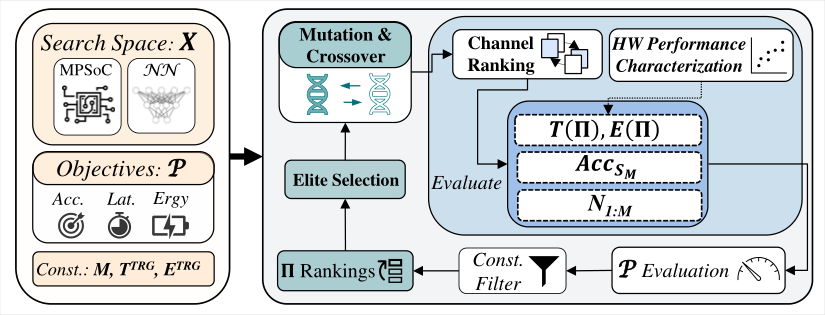
In this section, we propose an optimization framework to solve the mapping problem. Figure 5 gives an overview of our framework, whose key components are detailed below.
V-A Search Space
Here we describe how to generate a search space, of mapping strategy parameters, namely the space of (). Firstly, given a pretrained and an MPSoC with CUs, we can generate based on the ’s layer specifications and the MPSoC’s underlying hardware composition. For the former, the attainable depth and width parameters of every layer define the parameter matrices. For the latter, specifies its mapping space and the total number of inference stages. Lastly, is specified through the hardware reconfiguration parameters (DVFS). For instance, the mapping search space complexity of one layer from the Visformer [10] is , considering channel partitioning ratios, , and .
V-B Performance Objectives
Next, a performance objective needs to be designated as for the main optimization function in equation (15), to be specifically used for the candidate mapping evaluation. For our case, we used the following expression for :
| (16) |
In which is the baseline accuracy of the pretrained model; is the accuracy of the last stage of the dynamic version of as its base accuracy. The aforementioned terms are included to ensure that no accuracy drops ensue when a model’s structure changes through the matrix. represents the number of input samples -from the validation dataset- correctly classified at , given that every prior stage misclassifies them. is the latency experienced by the MPSoC at stage based on equation (9); is the energy consumed by the system as the result of executing stages of the model – each is evaluated as in equation (12).
V-C Search Algorithm
We develop an evolutionary-based algorithm to effectively explore the search space. Following the workflow in Figure 5, every new search iteration entails a new population, say . Then for every configuration , its corresponding dynamic and hardware settings are evaluated using a predefined objective function, . Based on results, configurations that do not meet the search constraints (e.g., memory usage) are omitted, whereas the remaining ones are ranked according to , and a subset of elite configurations is taken for a mutation and crossover stage to obtain the new population . Once the search budget expires, a Pareto set in calculated from all the generated populations from which the ideal dynamic mapping strategy is extracted.
V-D Channel Partitioning and Reordering
Before a candidate configuration is evaluated on the objective function , the should be partitioned according to the ratios in . Yet to maximize performance when partitioning, the width channels in each model layer are arranged according to their degree of importance. The logic being that given the sampled partitioning matrix for a configuration , it would be beneficial to assign the most important channels in the layer to the earlier inference stages for dynamic inference. This would enable numerous samples to terminate processing prematurely if deemed feasible, which will consequently aid in enhancing the dynamic inference performance of the with regards to experienced latency and energy on the MPSoC. This reordering method is feasible as all channels within the same layer share the same dimensions. Channel ranking is widely used for network pruning, and we follow the approach in [19] to estimate each channel’s importance.
|
|
|
|
|
| ||||||||||||
| Visformer (ViT-based Architecture) | |||||||||||||||||
| None | GPU | 88.09 | 197.35 | 15.01 | - | ||||||||||||
| DLA | 69.22 | 53.71 | - | ||||||||||||||
| No Fmap Constr. | Ours-L | 86.12 | 108.44 | 25.58 | 68.75 | ||||||||||||
| Ours-E | 87.58 | 59.21 | 30.40 | 61.25 | |||||||||||||
| 75% Fmap Constr. | Ours-L | 84.64 | 102.67 | 24.65 | 65.00 | ||||||||||||
| Ours-E | 87.67 | 65.12 | 29.46 | 75.00 | |||||||||||||
| 50% Fmap Constr. | Ours-L | 82.69 | 116.00 | 24.51 | 50.00 | ||||||||||||
| Ours-E | 84.16 | 82.44 | 32.70 | 50.00 | |||||||||||||
| VGG19 (CNN-based Architecture) | |||||||||||||||||
| None | GPU | 80.55 | 630.11 | 25.23 | - | ||||||||||||
| DLA | 164.89 | 114.41 | - | ||||||||||||||
| No Fmap Constr. | Ours-L | 84.81 | 251.63 | 25.67 | 52.94 | ||||||||||||
| Ours-E | 84.63 | 153.97 | 34.02 | 70.58 | |||||||||||||
| 75% Fmap Constr. | Ours-L | 84.76 | 247.34 | 26.07 | 64.70 | ||||||||||||
| Ours-E | 82.64 | 136.31 | 37.22 | 47.05 | |||||||||||||
| 50% Fmap Constr. | Ours-L | 84.62 | 250.80 | 25.83 | 50.00 | ||||||||||||
| Ours-E | 82.53 | 136.41 | 37.24 | 50.00 | |||||||||||||
V-E Performance Evaluation
Once a model is transformed to its dynamic version through and , the hardware measurements needed for the performance evaluation of each in equation (16) need to be estimated for each input sample. One way to achieve this is through surrogate models, which are able to predict and of each layer mapped onto stage (also CU ) based on input configurations while abiding by any inter-stage execution dependencies, and taking into account the computation cost and feature map communication overheads. Hence, a predictor (XGBoost [20] in our case) is first trained on a benchmarked dataset of diverse layer specifications, deployment hardware and DVFS settings. Afterwards, the predictor is deployed to characterize the performance of each model sampled within the population, providing estimates for its base latency, , and energy consumption, . In our case, we use the TensorRT library to first evaluate performance overheads on a layer-wise granularity, construct the dataset, and then deploy the predictor to provide hardware evaluations to involved models.
VI Experiments
VI-A Experimental Setup
Our experiments are conducted on the MPSoC provided by NVIDIA: Jetson AGX Xavier. This platform embeds CPU, GPU, and DLA cores on the same chip, sharing the same system memory. To run the workloads on the DLA, we use TensorRT and ONNX to build inference engines from the PyTorch model. As , we use Visformer [10] as ViT-based architecture and VGG19 [21] as CNN-based architecture to validate our approach for both cases. The dataset used for accuracy assessment is CIFAR100. Regarding the optimization framework, we run the optimization algorithm for 200 generations, each with a population size of 60, resulting in 12K overall evaluations. Furthermore, the evaluation step is performed on a cluster of 12 GPUs taking up to 10 GPU hours to run the entire optimization process.
VI-B Search Process Analysis

In this section, we analyze the results of the search process conducted by our framework under two main cases: 1) When no constraint is set to limit the feature map reuse between inference stages, 2) When only less than 75%, 50% of feature maps can be reused, respectively. In Figure 6, we show the optimization results for each case. Firstly, we observe that most of the explored configurations achieve a good tradeoff between DLA energy efficiency and GPU latency speedup. Furthermore, under the same baseline accuracy of Visformer, we notice an energy gain up to 2.1x compared to the GPU-only mapping with latency . Similarly, a latency speedup up to 1.7x compared to the DLA-only mapping, with comparable energy efficiency. Secondly, we can notice an accuracy drop of 6% when setting up hard constraints on the feature map reuse (See the 50% case). Hence, defining the optimal inter-stages concatenation strategy that determines the feature maps reuse ratio is crucial to maintain the desired level of accuracy while minimizing inter-CUs dependencies.
VI-C Pareto Optimal Models Analysis
In this section, we delve further into the performance breakdown of the Pareto optimal models obtained from the three search strategies. We select the most energy-oriented models and compare them with the baseline Visformer mapped entirely on the DLA. Figure 7 and Table II detail the obtained results. By exploring neural network dynamicity and concurrency on heterogeneous CUs, our models achieve better latency-energy tradeoff, providing latency speedup of 1.83x and up to 14.4% of energy gain as shown in the left sub-figure. In addition, the correlation between feature maps reuse and accuracy is highlighted in the right sub-figure. Reducing the feature maps reuse across stages decreases the inter-CUs data transmission at the cost of accuracy drops. However, some models can achieve comparable accuracy to the baseline while only reusing 60% of the necessary feature maps (See No constr. and 75% constr. cases)
VI-D Generalization to other architecture
To further demonstrate our approach’s applicability, we evaluate our optimization framework on a typical CNN architecture, VGG19. Table II details the obtained results. Regarding the baseline performances, VGG19 depicts a high energy consumption on GPU and slow execution latency on DLA. This is explained by its many weights and large feature maps, which entail high memory footprints for both CUs. Moreover, the large number of weights may exhibit a high degree of redundancy. Our approach has exploited these two properties of VGG19 well, resulting in up to 4.62x energy gain and 4.44x latency speedup. Furthermore, according to our analysis, more than 80% of samples were correctly classified in earlier stages with fewer channels, which results in considerable latency and energy gains.

VII Conclusion
We have presented Map-and-Conquer, an energy-efficient execution scheme for dynamic neural networks on heterogeneous MPSoCs by jointly optimizing the model partitioning along the width, hardware mapping, and DVFS. Map-and-Conquer’s awareness of the dynamicity and hardware computing units capabilities allows it to realize better performance trade-off over conventional single-platform mapping schemes. On CIFAR-100 and the AGX Xavier MPSoC, Map-and-Conquer achieved up to 2.1x energy gains over GPU-only mapping and up to 1.7x speedup over DLA-only mapping.
References
- [1] Y. Song et al., “Sara: Self-aware resource allocation for heterogeneous mpsocs,” in DAC, 2018.
- [2] M. A. H. Monil et al., “Mephesto: Modeling energy-performance in heterogeneous socs and their trade-offs,” in PACT, 2020, pp. 413–425.
- [3] Y. Xu et al., “Pccs: Processor-centric contention-aware slowdown model for heterogeneous system-on-chips,” in MICRO, 2021.
- [4] I. Dagli et al., “AxoNN: energy-aware execution of neural network inference on multi-accelerator heterogeneous SoCs,” in Proceedings of the 59th ACM/IEEE Design Automation Conference (DAC), 2022.
- [5] R. Hadidi et al., “Toward collaborative inferencing of deep neural networks on internet-of-things devices,” IEEE Internet of Things Journal, vol. 7, no. 6, pp. 4950–4960, 2020.
- [6] J. Mao et al., “Modnn: Local distributed mobile computing system for deep neural network,” in Design, Automation & Test in Europe Conference & Exhibition (DATE), 2017.
- [7] E. Shamsa et al., “Goal-driven autonomy for efficient on-chip resource management: Transforming objectives to goals,” in Design, Automation & Test in Europe Conference & Exhibition (DATE), 2019.
- [8] X. Hou et al., “Distredge: Speeding up convolutional neural network inference on distributed edge devices,” in IPDPS. IEEE, 2022.
- [9] Z. Yuan et al., “S2dnas: Transforming static cnn model for dynamic inference via neural architecture search,” in ECCV. Springer, 2020.
- [10] Z. Chen et al., “Visformer: The vision-friendly transformer,” in Proc. of the IEEE/CVF international conference on computer vision, 2021.
- [11] S. Teerapittayanon et al., “Branchynet: Fast inference via early exiting from deep neural networks,” in ICPR, 2016.
- [12] Y. Rao et al., “Dynamicvit: Efficient vision transformers with dynamic token sparsification,” NeurIPS, vol. 34, 2021.
- [13] Z. Yu et al., “Mia-former: Efficient and robust vision transformers via multi-grained input-adaptation,” in AAAI, vol. 36, no. 8, 2022.
- [14] E. Jeong et al., “Tensorrt-based framework and optimization methodology for deep learning inference on jetson boards,” ACM Transactions on Embedded Computing Systems (TECS), 2022.
- [15] D. Kang et al., “Scheduling of deep learning applications onto heterogeneous processors in an embedded device,” IEEE Access, vol. 8, 2020.
- [16] S.-C. Kao et al., “Gamma: Automating the hw mapping of dnn models on accelerators via genetic algorithm,” in ICCAD. IEEE, 2020.
- [17] H. Bouzidi et al., “HADAS: Hardware-Aware Dynamic Neural Architecture Search for Edge Performance Scaling,” in Design, Automation & Test in Europe Conference & Exhibition (DATE), 2023.
- [18] T. Tambe and al., “Edgebert: Sentence-level energy optimizations for latency-aware multi-task nlp inference,” in MICRO, 2021.
- [19] P. Molchanov et al., “Importance estimation for neural network pruning,” in CVPR, 2019.
- [20] T. Chen and C. Guestrin, “Xgboost: A scalable tree boosting system,” ser. KDD ’16, 2016.
- [21] K. Simonyan and A. Zisserman, “Very deep convolutional networks for large-scale image recognition,” in ICLR, Y. Bengio et al., Eds., 2015.