The virial theorem with periodic boundary conditions

The virial theorem Swenson 1983 relates averages of the kinetic energy to those of a function of the forces. For instance, for a particle confined in one-dimension described by position $x$ and momentum $p$

$$\left\langle p^{2}/m\right\rangle=\left\langle xdV/dx\right\rangle=-\langle xF\rangle$$

(1)

where the potential energy is $V(x)$ and the force on the particle is $F(x)$. The original derivation was dynamic, but we can also work from statistical mechanics looking at the average of the Poisson bracket $[G,H]$, where $H$ is the Hamiltonian of the system and $G=xp$. With $H=p^{2}/2m+V(x)$. The Poisson bracket is then

$$[G,H]=p\frac{\partial H}{\partial p}-x\frac{\partial H}{\partial x}=\frac{p^{2}}{m}-x\frac{\partial V}{\partial x}$$

(2)

and we recognize the two contributions to eq. (1). We choose to work in the canonical ensemble, appropriate for a molecular system coupled to a thermostat so that the statistical weight of a configuration is given by $e^{-\beta H}$. Let us consider, firstly, the kinetic contribution to the identity, $p^{2}/m$, using integration by parts.

	$\displaystyle\left\langle p\frac{\partial H}{\partial p}\right\rangle$	$\displaystyle=\frac{1}{Z_{p}}\int_{-\infty}^{\infty}p\frac{\partial H}{\partial p}e^{-\beta H}\,dp$		(3)
		$\displaystyle=-\frac{T}{Z_{p}}\int_{-\infty}^{\infty}dp\,p\frac{\partial e^{-\beta H}}{\partial p}=T$

We have introduced the temperature $T=\beta^{-1}$ and $Z_{p}$ is the kinetic contribution to the partition function. An identical transformation applies to the spatial derivative in the identity, $xdV/dx$, when the physical system is confined by the potential energy for $x\rightarrow\pm\infty$ so that integration by parts does not introduce a boundary contribution.

In a dilute gas identities such as eq. (1) find immediate application. There is a balance between the kinetic contribution, $\langle p^{2}/m\rangle$, and that due to the potential, $\langle xF\rangle$ which describes the interaction of atoms with confining walls. We now see an immediate problem with the application of the virial theorem in periodic systems: In the dilute-gas limit, there is no possibility of balancing the kinetic contribution with the wall collisions. Working in either toroidal space, or using replicated copies of a primary cell the classic formulation, assuming unbounded motion, requires modification. We note that the opposite limit of a dense, low temperature crystal was analyzed in Louwerse and Baerends 2006, where it was concluded that the calculation of the pressure requires a mathematical formulation which avoids entirely the classical virial theorem. This paper contains a strong criticism of formulations with replicated copies, which can mis-count contributions. Recent work and codes avoid the use of the virial theorem in periodic simulations, and uses alternative routes to the pressure Thompson et al. 2009.

In this paper we present a unified picture of the virial theorem valid for confined and periodic boundary conditions. We find extra boundary contributions (coming from integration by parts of the spatial derivative) that must be added to the classical result. These contributions, for instance, allow one to describe the dilute gas limit without contradiction. This formulation leads to a transparent formulation of the virial route to the pressure, linking the momentum transfer at the boundary of a simulation cell to the average volume virial.

In a second part we test our expressions in high statistics simulations with Monte Carlo and molecular dynamics studying a system of four particles in two dimensions. We find that the constraint of conservation of momentum in molecular dynamics leads to a non-uniform one-particle density that we study in detail.

We consider $N$ particles, in a $d$-dimensional periodic space. We allow the particles to interact with a short ranged, central pair-potential $v(\mathbf{r}_{i}-\mathbf{r}_{j})$ as well as an external one-body potential $\phi(\mathbf{r}_{i})$ so that

$$V=\sum_{i<j}v(\mathbf{r}_{i}-\mathbf{r}_{j})+\sum_{i}\phi(\mathbf{r}_{i})$$

(4)

We only consider systems in their toroidal representation so that $0\leq r_{i\alpha}<L_{\alpha}$, with $L_{\alpha}$ the box dimension in direction $\alpha$. The particles interact with a “minimum image” convention, so that the force is not always parallel to the vector $\mathbf{r}_{i}-\mathbf{r}_{j}$, but can rather be parallel to the vector

$$\Delta_{ij}=\mathbf{r}_{i}-\mathbf{r}_{j}-\textbf{L}_{n}$$

(5)

where the vector $\textbf{L}_{n}$ has entries $n_{\alpha}L_{\alpha}$ with $n_{\alpha}\in\{-1,0,1\}$. We consider short-range, smooth potentials so that interactions occur with at most a single value of the vector $\textbf{L}_{n}$. Use of the external potential $\phi$ will enable us to continuously pass from the case of an unconstrained periodic system with $\phi=0$, to a system with strong confining walls, so that we can compare the virial theorem in the two limits.

We introduce the partial virial $G_{x}=\sum_{i}x_{i}p_{i}$, with $p_{i}$ the $x$-component of the momentum for particle $i$. As in the one-dimensional case presented in the introduction, the treatment of the kinetic contribution to $\langle[G_{x},H]\rangle$ is elementary

$$\sum^{N}_{i}\left\langle p_{i}\frac{\partial H}{\partial p_{i}}\right\rangle=NT$$

(6)

More care is required for the treatment of the configurational average. Consider the term $x_{1}F^{x}_{1}$, with $F^{x}_{1}$ the $x$-component of the force on particle $1$: the partition function is defined as an integral over a finite interval of $x_{1}$. When performing the integration by parts, one must be careful not drop the boundary contribution.

$$\left\langle x_{1}\frac{\partial V}{\partial x_{1}}\right\rangle=-\frac{T}{Z_{r}}\int_{0}^{L_{x}}d^{N}\mathbf{r}\,x_{1}\frac{\partial}{\partial x_{1}}e^{-\beta V}$$

(7)

$Z_{r}$ is the spatial contribution to the partition function. We find two contributions

		$\displaystyle-\frac{T}{Z_{r}}\left(\int_{0}^{L_{x}}d^{N-1}\mathbf{r}\,{[x_{1}e^{-\beta V}]}_{x_{1}=0}^{x_{1}=L_{x}}-\int_{0}^{L_{x}}d^{N}\mathbf{r}\,e^{-\beta V}\right)$		(8)
		$\displaystyle=-TL_{x}\bar{\rho}_{1}(x_{1}=L_{x})+T$

where $\bar{\rho}_{1}(x_{1}=0)\equiv\bar{\rho}_{1}(x_{1}=L_{x})$ is the one-particle density, $\rho(\mathbf{r})=\langle\delta(\mathbf{r}-\mathbf{r}_{1})\rangle$, integrated over the boundary $x=L_{x}$ of the fundamental cell.

Thus, the full periodic version of the virial theorem in the $x$-direction is

$$\sum_{i}\left\langle\frac{{p_{i}}^{2}}{m}+x_{i}F^{x}_{i}\right\rangle=TL_{x}\bar{\rho}_{N}(x=L_{x})$$

(9)

with $\bar{\rho}_{N}(x=L_{x})$ the integrated density of the $N$ particles over the wall at $x=L_{x}$. The limit of weak potentials is now reasonable because then $\bar{\rho}_{N}(x=L_{x})=N/L_{x}$ and the theorem now allows finite kinetic energy in the limit $V\rightarrow 0$: We find the clearly correct result $\sum_{i}p_{i}^{2}/m=NT$

For periodic systems, with $\phi=0$ but with $v(\mathbf{r})$ not zero, the average of the kinetic energy and the boundary contribution cancel, and we find that the average configurational virial vanishes.

$$\sum_{i}{\left\langle x_{i}\frac{\partial V}{\partial x_{i}}\right\rangle}_{\phi=0}=0$$

(10)

However, when we impose a large positive potential $\phi$ at the boundary of the simulation cell then $\bar{\rho}_{N}(x=L_{x})$ is small and the result eq. (9) reduces to the confined limit, eq. (1). Eq. (10) is compatible with the statements in Louwerse and Baerends 2006 where a perfect crystal at zero temperature is analyzed. The authors show that use of eq. (10) in the wrong context leads to the conclusion that such crystal is always at pressure $P=0$.

It is conventional to re-write the potential part of the virial for pair potentials in a form which is independent of the origin of the system. We do this by breaking up the total force on particle $i$ due to the potential $v$ in the following manner. $f^{x}_{i}=\sum_{j}f^{x}_{ij}$ where $f^{x}_{ij}$ denotes the $x$-component of the pair force on particle $i$ due to $j$, and $f^{x}_{i}$ is the $x$-component of the total pair force. Then,

$$\sum^{N}_{i}x_{i}f^{x}_{i}=\sum^{N}_{i\neq j}x_{i}f^{x}_{ij}$$

(11)

Note it is always true that $f^{x}_{ij}=-f^{x}_{ji}$ even if, Fig. (1), the interactions occur with images outside the primitive cell so that

$$\sum^{N}_{i}x_{i}f^{x}_{i}=\frac{1}{2}\sum^{N}_{i\neq j}(x_{i}-x_{j})f^{x}_{ij}$$

(12)

We now re-write eq. (12) in terms of nearest image interactions using $\Delta_{ij}$, eq. (5), together with a boundary term and find

$$\sum^{N}_{i}x_{i}f^{x}_{i}=\frac{1}{2}\sum^{N}_{i\neq j}(\Delta_{ij,x}f^{x}_{ij}+n_{x}L_{x}f^{x}_{ij})$$

(13)

We thus write eq. (9) as

	$\displaystyle NT$	$\displaystyle+\frac{1}{2}\sum^{N}_{i\neq j}\left\langle\Delta_{ij}f^{x}_{ij}\right\rangle-\sum^{N}_{i}\langle x_{i}\frac{\partial\phi}{\partial x_{i}}\rangle$		(14)
		$\displaystyle=TL_{x}\bar{\rho}_{N}(L_{x})-L_{x}\left\langle\sum_{\parbox{24.58342pt}{\tiny boundary pairs}}f^{x}_{ij}n_{x}\right\rangle$		(15)
		$\displaystyle=\Omega P_{x}$		(16)

We now interpret the contributions to eq. (14, 15). Eq. (14) contains the usual Irving-Kirkwood Irving and Kirkwood 1950 stress tensor evaluated with a nearest image convention together with a body force imposed by $\phi$. Eq. (15) corresponds to momentum flux through the boundary $(x=L_{x})$, giving the $x$-component of the pressure $P_{x}$ in a system of volume $\Omega$. There are two contributions to this momentum flux, a part due to particles crossing the boundary, $T\bar{\rho}_{N}(L_{x})$, as well as a contribution involving forces between particles which are on two different sides of the boundary in the nearest image convention, Fig. (1). The combination $f^{x}_{ij}n_{x}$ with now $n_{x}\in\{-1,1\}$ orients the force through the boundary, independent of the labeling order $ij$. In Fig. (1), for the rightmost boundary, when $i$ is inside the cell, and $j^{\prime}$ outside $n_{x}=1$. The position of the boundary in our derivation is arbitrary, so that eq. 15) holds for an arbitrary choice of origin.

Again, we see that including the boundary term, arising from integration by parts is essential for the correct link between the volume expression for the stress tensor, and the momentum flux through the boundary of the simulation cell, and thus the $x$-component of the pressure. Note the stress tensor, $\sigma$ and thus the pressure is not constant in the presence of a general one-body potential Davis and Scriven 1982, as is implied by the Yvon-Born-Green equation linking one-particle and two-particle correlations.

The derivation of the virial in periodic systems often works from a dynamic approach, rather than the statistical approach used here Erpenbeck and Wood 1984; Tsai 1979. This formulation follows the particles originating in one copy of the simulation cell, now in the micro-canonical ensemble obeying Newton’s equation of motion, without folding the particles back when they leave the fundamental copy. One looks at the time derivative of $G_{x}$ using the equations of motion, and then argues that since motions and energies are bounded

$$\lim_{t\to\infty}\frac{1}{t}\int_{0}^{t}\dot{G}_{x}(\tau)\,d\tau=0$$

(17)

If we follow the trajectories of particles, without folding them back into the primary simulation domain, we find (see for instance Erpenbeck and Wood 1984; Winkler et al. 1992) a result similar to eq. (15), with however important differences. Firstly, the boundary contribution in $T\bar{\rho}_{N}$ is entirely missing, secondly the contribution $L_{n}f^{x}_{ij}$ requires the uses of arbitrary large integers $n_{\alpha}\in\mathbb{Z}$ to push particles that have moved large distances back into the primary cell in order to calculate the system energy. In this limit it is impossible to recognize the result as expressing the momentum flux evaluated at the boundary of the simulation cell.

We now show that by confining particles to the primary cell, and periodically “transporting” them when they cross the cell boundary we also find the same formulation of the virial theorem eq. (9). We write

$$\frac{dG_{x}}{dt}=\sum_{i}(\dot{x}_{i}p_{i}+x_{i}\dot{p}_{i})=\sum_{i}\left(\frac{p_{i}^{2}}{m}+x_{i}F^{x}_{i}\right)$$

(18)

for time intervals where no particle leaves the primary domain. We define the temperature from the average kinetic energy, so that $\langle p_{i}^{2}/m\rangle=T$. For a system that undergoes molecular dynamics evolution with bounded forces then there is also a discontinuity in $x_{i}p_{i}$ each time a particle leaves the simulation cell, for instance at $x=L_{x}$ and is transported to $x=0$. We thus need to add to eq. (18) the extra contribution $-p_{i}L_{x}\delta(t-t_{r})$ where $t_{r}$ is the time the particle leaves to the right. A similar term is present when the particles leave to the left. Taking the time average of eq. (18) and noting that the left-hand side averages to zero, eq. (17)

$$\sum_{i}\left\langle\frac{p_{i}^{2}}{m}+x_{i}F^{x}_{i}\right\rangle=\frac{L_{x}}{t}\left[\sum_{t_{r}}p_{r}-\sum_{t_{l}}p_{l}\right]$$

(19)

where $p_{r}$ and $p_{l}$ is the momentum transported leaving the cell on the right or left. $p_{r}$ and $-p_{l}$ are both positive. The sums on the right are over all events where a particle leaves the primary domain. We now note this momentum flux is just the perfect gas stress contribution $T\bar{\rho}_{N}$ to the pressure, and we find an expression identical to eq. (9).

We now consider in more detail the limit of a small number of particles Hoover and Alder 1967; Ray and Zhang 1999; Wood et al. 2000, and show detailed calculations for $N=4$ with hard disks where efficient event driven methods are used to generate high statistics data Michel et al. 2014; Li et al. 2022. These simulations allow us to validate the expressions that we have found from the virial theorem. We first simulate with event-chain Monte Carlo to find a reference value of the pressure. For particles of radius $\sigma=0.15$ in a unit periodic cell, Fig. (2), we find $\beta PV=7.120986(9)$. We separate the pressure into a perfect gas contribution, $\beta VP^{perf}=4$, and a virial contribution $\beta VP^{vir}=3.120986(9)$.

In our molecular dynamics simulations we randomly initialize the velocities, and remove the center of mass motion. We then scale velocities of particles so that

$$\sum_{i}\frac{\textbf{v}_{i}^{2}}{2}=T(N-1)$$

(20)

where we take the particles masses, $m=1$. We note that the perfect gas limit of the pressure in molecular dynamics with periodic boundary conditions is

$$P=\frac{T}{V}(N-1)=T\rho\frac{(N-1)}{N}$$

(21)

since we work in the center of mass frame of the system. In this we diverge from historic papers on the small $N$ limit, where the temperature in molecular dynamics is defined from $PV=NT$ for a dilute gas.

There are two routes available to evaluate the pressure in molecular dynamics. The first, eq. (15), is the sum of the momentum transfer from collisions across the cell boundary (for instance a collision between $i$ and $j^{\prime}$ in Fig. (1)), plus the momentum flux due to particles travelling through the boundary which we evaluate with the right-hand side of eq. (19). We find $\beta PV=3+3.120995(9)$. Where we have again separated the perfect gas eq. (21) and virial contributions. The virial contribution is identical, within statistical errors, to that found given by Monte Carlo methods. We also checked that the contribution to the momentum flux due to particles crossing the boundary corresponds to the term $T\bar{\rho}_{N}(L_{x})$ in eq. (15) with the modification of eq. (21). The transport momentum flux is thus $T\bar{\rho}_{N}(L_{x})(N-1)/N$.

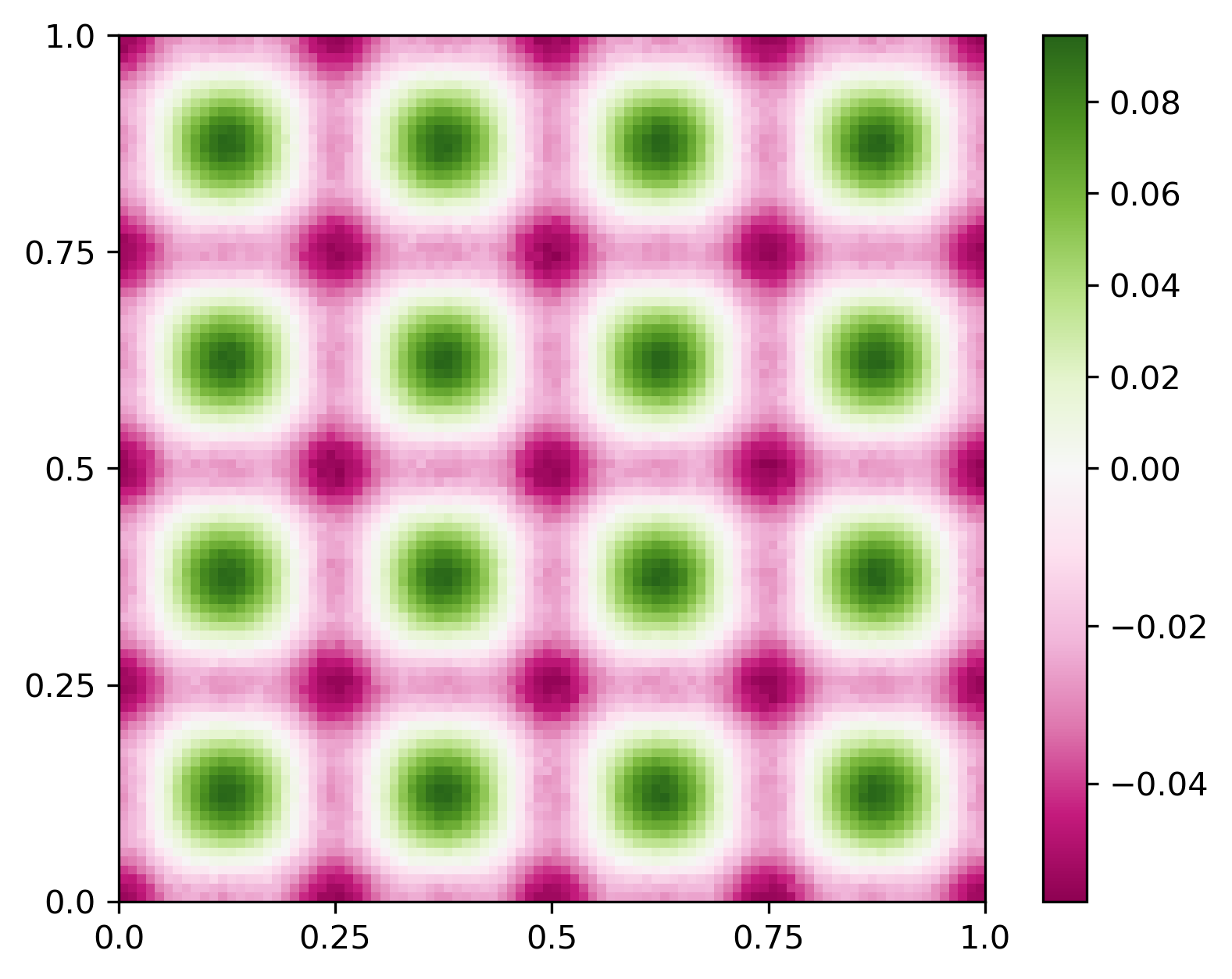
When examining our simulations, we found that although the sum of the two contributions to the pressure is statistically constant throughout the simulation cell, the magnitude of each contribution depends on the initial conditions of the simulation and is inhomogeneous in space. We investigated the variation in the two contributions to the pressure in detail and found, (Fig. (3)), that a histogram of particle positions is non-uniform. When working with $N$ particles we find a grid of $N\times N$ peaks in the density. We interpret this inhomogeneity as being due to the conservation of the position of the center of mass in molecular dynamics simulation: When a single particle moves to the right by a distance $L_{x}(1-1/N)$ and all other particles move to the left by a distance $L_{x}/N$ we generate an equivalent configuration with the same center of mass, that appears shifted left by $L_{x}/N$. Each peak in the grid of Fig. (3) corresponds to configurations with the same relative positions of all particles. Depending on the position of the center of mass with respect to the cell boundaries at the start of the simulation, the two contributions to the momentum flux vary while their sum remains identical.

The second route to the pressure in molecular dynamics is through the time averaged virial eq. 14, with again the perfect gas expression $NT$, replaced with $(N-1)T$. In our molecular dynamics simulations the virial and momentum routes to the pressure agree to one part in $10^{10}$, confirming the correctness of our derivation of the periodic theorem, and its application in a system with non-trivial spatial structure.

We are able to follow in our binning procedure the pattern of $N^{2}$ peaks up to $N=6$ (working at constant volume fraction of particles), the amplitude of the pattern becomes rapidly smaller with increasing $N$. We also confirmed the structure for $N=7$ with Fourier analysis. We were also able to study the pattern of peaks in our event-chain Monte Carlo code by measuring the density in a reference frame moving with the center of mass, then folding positions back into a co-moving simulation cell. Non-trivial density patterns occur in Monte Carlo when measured in the correct reference frame. Increasing the particle size leads a to a more complicated pattern, Fig. (4) of density variations.

We now demonstrate, under the usual hypothesis of factorization of velocity and spatial degrees of freedom, that the kinetic virial from molecular dynamics and the thermodynamic virial measured in Monte Carlo simulation are identical when using the correct link between temperature and kinetic energy, eq. (20). We use the approach of Li et al. 2022, section III.c.2, where the pressure is calculated in a thermodynamic approach. If $\hat{g}(r)$ is the probability density for finding a given pair of particles near separation $r$, then the contribution to the pressure coming from pair interactions is

$$\beta P^{vir}=\frac{N(N-1)}{V}2\pi\sigma^{2}\hat{g}(2\sigma)$$

(22)

The kinetic virial as measured in a molecular dynamics simulation for hard disks is given by

$$P^{vir}=-\frac{1}{2V}\left\langle(\textbf{v}_{i}-\textbf{v}_{j})\cdot(\textbf{r}_{i}-\textbf{r}_{j})\right\rangle$$

(23)

where the expectation is a time average of pair collisions between pairs of particles $i$ and $j$. This time average is calculated by averaging over the flux of collisions, $f$:

$$f=\frac{N(N-1)}{2}2\pi(2\sigma)\hat{g}(2\sigma)\frac{\big[{v^{r}}_{1}-{v^{r}}_{2}\big]}{2}H(\textbf{v})$$

(24)

Where $H(\textbf{v})$ is a uniform distribution of $2N$ velocity components on the hypersphere, confined to $\sum_{i}\textbf{v}_{i}=0$ and $\big[{v^{r}}_{1}-{v^{r}}_{2}\big]$ is the radial component of the relative velocity of two particles. The contribution to the pressure is thus

$$P^{vir}=\frac{N(N-1)}{4V}2\pi{(2\sigma)}^{2}\hat{g}(2\sigma)\left\langle\frac{{\big[{v^{r}}_{1}-{v^{r}}_{2}\big]}^{2}}{2}H(\textbf{v})\right\rangle$$

(25)

The velocity average is calculated by noting that $\left\langle{v^{r}}_{1}{v^{r}}_{2}H(\textbf{v})\right\rangle=-\langle{({v^{r}}_{1})}^{2}H(\textbf{v})\rangle/(N-1)$ so that

$$P^{vir}=\frac{N(N-1)}{4V}2\pi{(2\sigma)}^{2}{\hat{g}}(2\sigma)\left\langle{(v^{r}_{1})}^{2}H(\textbf{v})\right\rangle\frac{N}{N-1}$$

(26)

Consistency between eqs. (26, 22) requires

$$\left\langle\frac{\textbf{v}_{i}^{2}}{2}\right\rangle=\frac{N-1}{N}T$$

(27)

as used in our simulations.

We have treated the generalization of the virial theorem to periodic systems using two approaches. Firstly, using ensemble averages from equilibrium statistical mechanics, secondly using a dynamical approach from the equations of motion. Our approach avoids the difficulties carefully pointed out in Louwerse and Baerends 2006, which lead to nonsensical results for the pressure, when starting from classical statements of the theorem.

Our treatment of the virial theorem has features that are similar to the quantum virial theorem treated in Abad and Esteve 1991; Esteve et al. 2012. Again, the use of a periodic space in quantum mechanics leads to extra end-corrections to the theorem, here involving boundary values of the wavefunction. Our treatment deals cleanly with the weakly interacting gas limit, which is clearly not correctly given using the classical virial expression. Using an external one-body potential, we interpolate between the standard confined simulation box, and a system where particles move freely through cell boundaries. This one-body potential can describe either a high uniform wall, or more complicated geometries such as a hole in an otherwise impenetrable barrier. Our expression gives a direct link between the Irving-Kirkwood expression for the stress tensor and the boundary momentum flux. We checked the use of our virial and momentum estimators for the case of $N=4$ particles, and compared the results to independent event-chain Monte Carlo simulations.

Open questions remain for the formulation of the virial for long-ranged electrostatic interactions. The most natural formulation of electrostatics boundary conditions requires the use of a non-periodic representation of the particle positions in order to correctly represent the molecular polarization of charged media Caillol 1994; Maggs 2004; Sprik 2018; Maggs 2002; Maggs 2012.

I would like to thank Werner Krauth for the many discussions that formed the starting point of this work.

References

- Abad and Esteve (1991) Abad, J, and J. G. Esteve (1991), “Generalized virial theorem for compact problems,” Phys. Rev. A 44, 4728–4729.
- Caillol (1994) Caillol, Jean‐Michel (1994), “Comments on the numerical simulations of electrolytes in periodic boundary conditions,” The Journal of Chemical Physics 101 (7), 6080–6090.
- Davis and Scriven (1982) Davis, H T, and L. E. Scriven (1982), “Stress and structure in fluid interfaces,” in Advances in Chemical Physics (John Wiley & Sons, Ltd) pp. 357–454.
- Erpenbeck and Wood (1984) Erpenbeck, Jerome J, and William W. Wood (1984), “Molecular dynamics calculations of the hard-sphere equation of state,” Journal of Statistical Physics 35 (3), 321–340.
- Esteve et al. (2012) Esteve, J G, F. Falceto, and Pulak Ranjan Giri (2012), “Boundary contributions to the hypervirial theorem,” Phys. Rev. A 85, 022104.
- Hoover and Alder (1967) Hoover, William G, and Berni J. Alder (1967), “Studies in molecular dynamics. iv. the pressure, collision rate, and their number dependence for hard disks,” The Journal of Chemical Physics 46 (2), 686–691.
- Irving and Kirkwood (1950) Irving, J H, and John G. Kirkwood (1950), “The statistical mechanical theory of transport processes. iv. the equations of hydrodynamics,” The Journal of Chemical Physics 18 (6), 817–829.
- Li et al. (2022) Li, Botao, Yoshihiko Nishikawa, Philipp Höllmer, Louis Carillo, A. C. Maggs, and Werner Krauth (2022), “Hard-disk pressure computations—a historic perspective,” The Journal of Chemical Physics 157 (23), 234111.
- Louwerse and Baerends (2006) Louwerse, Manuel J, and Evert Jan Baerends (2006), “Calculation of pressure in case of periodic boundary conditions,” Chemical Physics Letters 421 (1), 138–141.
- Maggs (2002) Maggs, A C (2002), “Dynamics of a local algorithm for simulating Coulomb interactions,” The Journal of Chemical Physics 117 (5), 1975–1981, https://doi.org/10.1063/1.1487821 .
- Maggs (2004) Maggs, A C (2004), “Auxiliary field Monte Carlo for charged particles,” The Journal of Chemical Physics 120 (7), 3108–3118.
- Maggs (2012) Maggs, A C (2012), “A minimizing principle for the Poisson-Boltzmann equation,” Europhysics Letters 98 (1), 16012.
- Michel et al. (2014) Michel, Manon, Sebastian C. Kapfer, and Werner Krauth (2014), “Generalized event-chain monte carlo: Constructing rejection-free global-balance algorithms from infinitesimal steps,” The Journal of Chemical Physics 140 (5), 054116.
- Ray and Zhang (1999) Ray, John R, and Hongwei Zhang (1999), “Correct microcanonical ensemble in molecular dynamics,” Phys. Rev. E 59, 4781–4785.
- Sprik (2018) Sprik, M (2018), “Finite Maxwell field and electric displacement Hamiltonians derived from a current dependent Lagrangian,” Molecular Physics 116 (21-22), 3114–3120.
- Swenson (1983) Swenson, Robert J (1983), “Comments on virial theorems for bounded systems,” American Journal of Physics 51 (10), 940–942.
- Thompson et al. (2009) Thompson, Aidan P, Steven J. Plimpton, and William Mattson (2009), “General formulation of pressure and stress tensor for arbitrary many-body interaction potentials under periodic boundary conditions,” The Journal of Chemical Physics 131 (15), 154107.
- Tsai (1979) Tsai, D H (1979), “The virial theorem and stress calculation in molecular dynamics,” The Journal of Chemical Physics 70 (3), 1375–1382.
- Winkler et al. (1992) Winkler, RG, H. Morawitz, and D.Y. Yoon (1992), “Novel molecular dynamics simulations at constant pressure,” Molecular Physics 75 (3), 669–688.
- Wood et al. (2000) Wood, William W, Jerome J. Erpenbeck, George A. Baker, and J. D. Johnson (2000), “Molecular dynamics ensemble, equation of state, and ergodicity,” Phys. Rev. E 63, 011106.