Wigner State and Process Tomography on Near-Term Quantum Devices

A general procedure for performing tomography in the context of Wigner representations using a scanning approach is described in the study [Leiner et al.(2017)Leiner, Zeier, and Glaser] (see results 1 and 2). Here we summarize this approach. In the following, we focus without loss of generality on a system consisting of $N$ qubits. Consider a multi-qubit quantum operator $A$, which is also represented by a set of rank $j$ and label $\ell$ spherical droplet functions $f^{(\ell)}=\sum_{j\in J(\ell)}f^{(\ell)}_{j}(\beta,\alpha)$ as described in Sec. S-I. To distinguish the size of different matrices, in the following, we refer to operators as $A^{[N]}$, where $N$ is the number of qubits and therefore, the operator $A^{[N]}$ is represented by a matrix of size $2^{N}\times 2^{N}$. The main aim is to experimentally measure spherical droplet functions $f^{(\ell)}_{j}$ representing a quantum operator $A$ and this can be done by experimentally estimating the scalar products of rotated axial tensor operators $T_{j,\alpha\beta}^{(\ell)[N]}$ with operator $A^{[N]}$, where

$$T_{j,\alpha\beta}^{(\ell)[N]}=R_{\alpha\beta}^{[N]}(T_{j0}^{(\ell)})^{[N]}(R_{\alpha\beta}^{[N]})^{\dagger}.$$

(1)

The term $(T_{j,\alpha\beta}^{(\ell)})^{[N]}$ is the rotated version of axial tensor operators $(T_{j0}^{(\ell)})^{[N]}$ of rank $j$ and order $m=0$. The rotation operator is given by

$$R_{\alpha\beta}^{[N]}=\text{exp}(-i\alpha F_{z}^{[N]})\text{exp}(-i\beta F_{y}^{[N]})$$

(2)

where $F_{z}=\frac{1}{2}\sum_{k=1}^{N}\sigma_{kz}^{[N]}$, and $F_{y}=\frac{1}{2}\sum_{k=1}^{N}\sigma_{ky}^{[N]}$. $R_{\alpha\beta}^{[N]}$ corresponds to a rotation around the $y$ axis by polar angle $\beta\in[0,\pi]$ followed by rotation around the $z$ axis by azimuthal angle $\alpha\in[0,2\pi)$. Here we use the shorthand notation $\sigma_{ka}=\mathds{1}\otimes\dots\otimes\mathds{1}\otimes\sigma_{a}\otimes\mathds{1}\otimes\dots\otimes\mathds{1}$, where $\sigma_{a}$ is located on the $k^{th}$ position and $a\in\{x,y,z\}$. For given angles $\beta$ and $\alpha$, droplet function $f_{j}^{(\ell)}$ can be calculated by

$$f_{j}^{(\ell)}(\beta,\alpha)=s_{j}\langle{T_{j,\alpha\beta}^{(\ell)[N]}}|{A^{[N]}}\rangle,$$

(3)

which can be equivalently written using a shorthand notation as

$$f_{j}^{(\ell)}(\beta,\alpha)=s_{j}\langle{T_{j,\alpha\beta}^{(\ell)[N]}}\rangle_{A^{[N]}},$$

(4)

where $s_{j}=\sqrt{(2j+1)/(4\pi)}$ and the scalar product $\langle{T_{j,\alpha\beta}^{(\ell)[N]}}|{A^{[N]}}\rangle$ is expressed as the expectation value of $T_{j,\alpha\beta}^{(\ell)[N]}$ for the density operator ${A^{[N]}}$:

$$\langle{T_{j,\alpha\beta}^{(\ell)[N]}}\rangle_{A^{[N]}}=\text{tr}\big\{(T_{j,\alpha\beta}^{(\ell)[N]})A^{[N]}\big\}.$$

(5)

Note that axial tensor operators are Hermitian, i.e., $({T_{j,\alpha\beta}^{(\ell)[N]}})^{\dagger}=({T_{j,\alpha\beta}^{(\ell)[N]}})$ [Leiner et al.(2017)Leiner, Zeier, and Glaser].

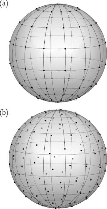
For the experimental tomography of droplet functions $f_{j}^{(\ell)}(\beta,\alpha)$ using the scanning approach, a multitude of choices for the set of sampling angles $\beta$ and $\alpha$ can be used. Fig. 5 illustrates two such sampling techniques: equiangular and REPULSION [Bak and Nielsen(1997)]. For simplicity, in the demonstration experiments shown here, we use an equiangular grid, but a numerical study using more sophisticated sampling techniques is presented and discussed in Sec. 8.

In this section, we first present an algorithm for Wigner quantum state tomography and then elaborate each step individually. A general step-wise procedure (see Fig. 6) to experimentally measure a spherical droplet function $f^{(\ell)}_{j}$ representing a density matrix $\rho^{[N]}=|\psi^{[N]}\rangle\langle\psi^{[N]}|$ is the following:

1. (i)

   Preparation ($\mathcal{P}$): Prepare the desired quantum state $\rho^{[N]}$ from a defined initial state $\rho_{i}^{[N]}$.

2. (ii)

   Rotation ($\mathcal{R}$): Rotate the density operator $\rho^{[N]}$ inversely for scanning.

3. (iii)

   Detection-associated rotations ($\mathcal{D}$): Apply local unitary operations to measure expectation values of Pauli operator components of axial tensor operators $T_{j0}^{(\ell)[N]}$ (see Table 1) that are not directly measurable.

These steps are repeated for the set of angles $\beta\in[0,\pi]$, $\alpha\in[0,2\pi]$ and for different local unitary operators $u_{n}$ (vide infra), rank $j$, and label $\ell$ to experimentally scan the droplet functions $f_{j}^{(\ell)}$. In the rest of this section, we elaborate on each step of the presented algorithm.

Step 1: The first step of the algorithm, ‘Preparation’, can be achieved by applying unitary operations depending on the initial and desired state.

Step 2: Since our operator of interest is a density matrix $\rho^{[N]}$, Eq. 4 takes the following form:

$$f_{j}^{(\ell)}(\beta,\alpha)=s_{j}\langle{T_{j,\alpha\beta}^{(\ell)[N]}}\rangle_{\rho^{[N]}}.$$

(6)

Instead of rotating the axial tensor operators $T_{j0}^{(\ell)[N]}$ as shown in Eq. 1, it is equivalent (and experimentally more convenient) to rotate the density matrix $\rho^{[N]}$ inversely, such that:

$$f_{j}^{(\ell)}(\beta,\alpha)=s_{j}\langle{T_{j0}^{(\ell)[N]}}\rangle_{\tilde{\rho}^{[N]}},$$

(7)

where

$$\tilde{\rho}^{[N]}=(R_{\alpha\beta}^{[N]})^{-1}\rho^{[N]}R_{\alpha\beta}^{[N]}.$$

(8)

The axial tensor operators $(T_{j0}^{(\ell)})$ are explicitly given in [Garon et al.(2015)Garon, Zeier, and Glaser, Leiner et al.(2020)Leiner, Zeier, and Glaser] for systems consisting of up to six qubits. In Table 1, we summarize the axial tensor operators for one and two-qubit systems.

Step 3: Depending on the number of qubits $N$ and rank $j$, the axial tensors $T_{j0}^{(\ell)}$ consist of different Pauli operators (see Table 1), but it might not be possible to measure these components directly depending on the specific quantum computing hardware. In a typical pure-state quantum computing device, the measurement is done along the $z$ axis, which implies that the directly measurable operators are: $\mathds{1}$, $\sigma_{1z}$, $\sigma_{2z}$, and $\sigma_{1z}\sigma_{2z}$. In this case, measuring expectation values of non-directly measurable operators can be achieved with the help of local unitary operations $u_{n}$. For example, consider the expectation value $\langle T_{10}^{(12)}\rangle_{\tilde{\rho}(\beta,\alpha)}$ given by:

	$\displaystyle\langle T_{10}^{(12)}\rangle_{\tilde{\rho}(\beta,\alpha)}$	$\displaystyle=\frac{1}{2\sqrt{2}}\langle{\sigma_{1x}\sigma_{2y}-\sigma_{1y}\sigma_{2x}\rangle}_{\tilde{\rho}(\beta,\alpha)}$		(9)
		$\displaystyle=\frac{1}{2\sqrt{2}}\langle{\sigma_{1x}\sigma_{2y}}\rangle_{\tilde{\rho}(\beta,\alpha)}-\frac{1}{2\sqrt{2}}\langle{\sigma_{1y}\sigma_{2x}}\rangle_{\tilde{\rho}(\beta,\alpha)}.$

In the first term ($n=1$) of Eq. 9, the expectation value $\langle{\sigma_{1x}\sigma_{2y}}\rangle_{\tilde{\rho}(\beta,\alpha)}$ needs to be determined. This can be achieved by measuring instead the expectation value

$$\langle{\sigma_{1z}\sigma_{2z}}\rangle_{\tilde{\rho}_{1}(\beta,\alpha)}=\langle{\sigma_{1x}\sigma_{2y}}\rangle_{\tilde{\rho}(\beta,\alpha)},$$

(10)

where

$$\tilde{\rho}_{1}(\beta,\alpha)=u_{1}\tilde{\rho}(\beta,\alpha)u_{1}^{\dagger}.$$

(11)

The density operator $\tilde{\rho}_{1}(\beta,\alpha)$ is obtained from $\tilde{\rho}(\beta,\alpha)$ by applying a $-\pi/2$ rotation around the $y$ axis (for bringing the $x$ axis to the $z$ axis) to the first qubit and a $\pi/2$ rotation around the $x$ axis (for bringing the $y$ axis to the $z$ axis) to the second qubit. This corresponds to the local unitary transformation $u_{1}=\big((R_{0,\frac{\pi}{2}})^{-1}\otimes\mathds{1}\big)\cdot(\mathds{1}\otimes(R_{\frac{\pi}{2},\frac{\pi}{2}})^{-1})$.

Similarly, in the second term ($n=2$) of Eq. 9, the expectation value $\langle{\sigma_{1y}\sigma_{2x}}\rangle_{\tilde{\rho}(\beta,\alpha)}$ needs to be determined. This can be achieved by measuring instead the expectation value

$$\langle{\sigma_{1z}\sigma_{2z}}\rangle_{\tilde{\rho}_{2}(\beta,\alpha)}=\langle{\sigma_{1y}\sigma_{2x}}\rangle_{\tilde{\rho}(\beta,\alpha)},$$

(12)

where

$$\tilde{\rho}_{2}(\beta,\alpha)=u_{2}\tilde{\rho}(\beta,\alpha)u_{2}^{\dagger}.$$

(13)

The density operator $\tilde{\rho}_{2}(\beta,\alpha)$ is obtained from $\tilde{\rho}(\beta,\alpha)$ by applying a $\pi/2$ rotation around the $x$ axis (for bringing the $y$ axis to the $z$ axis) to the first qubit and a $-\pi/2$ rotation around the $y$ axis (for bringing the $x$ axis to the $z$ axis) to the second qubit. This corresponds to the local unitary transformation $u_{2}=\big((R_{{\frac{\pi}{2}},\frac{\pi}{2}})^{-1}\otimes\mathds{1}\big)\cdot(\mathds{1}\otimes(R_{0,\frac{\pi}{2}})^{-1})$.

Overall, for $\ell=\{12\}$ and $j=1$, the droplet function from Eq. 7 can be expressed as

	$\displaystyle f_{1}^{(12)}(\beta,\alpha)$	$\displaystyle=s_{1}\langle T_{10}^{(12)}\rangle_{\tilde{\rho}(\beta,\alpha)}$		(14)
		$\displaystyle=\frac{s_{1}}{2\sqrt{2}}(\langle{\sigma_{1z}\sigma_{2z}}\rangle_{\tilde{\rho}_{1}(\beta,\alpha)}+\langle{\sigma_{1z}\sigma_{2z}}\rangle_{\tilde{\rho}_{2}(\beta,\alpha)}).$

Hence, only projective measurements along the $z$ axis are required, c.f. S-III.

In this section, we show how the matrix form of a density operator can be estimated based on its experimentally measured DROPS representation. A general $N$-qubit density matrix [Nielsen and Chuang(2010)] can be expressed in terms of Pauli operators as:

$$\rho^{[N]}=\sum_{a=0}^{3}\sum_{b=0}^{3}\dots\sum_{g=0}^{3}r_{ab\dots g}(\sigma_{a}\otimes\sigma_{b}\otimes\dots\otimes\sigma_{g})$$

(15)

where $\sigma_{0}$ is $\mathds{1}$ (the 2$\times$2 identity matrix), while $\sigma_{1},\sigma_{2}$, and $\sigma_{3}$ are standard Pauli matrices $\sigma_{x},\sigma_{y}$, and $\sigma_{z}$ respectively. The terms $r_{ab\dots g}$ are real coefficients. Given the DROPS representation of a density operator, these coefficients can be computed by calculating the scalar product between basis droplets (ideally simulated without noise) and experimental droplets [Leiner et al.(2017)Leiner, Zeier, and Glaser]. The basis droplets can be generated using the definitions provided in supplementary Sec. S-VI for one and two qubits.

The scalar product between two tensor operators can be approximated by the discretized scalar product between their droplet functions, see supplementary Sec. S-II. In the general case of a droplet $f_{A}$ with complex values $f_{A}(\theta_{i},\phi_{i})$ and another droplet $f_{B}$ with complex values $f_{B}(\theta_{i},\phi_{i})$ at the grid points, the scalar product or overlap between the two droplets is given by

$$r=\langle f_{A}|f_{B}\rangle=\sum_{i}\text{w}_{i}f_{A}^{*}(\theta_{i},\phi_{i})f_{B}(\theta_{i},\phi_{i}),$$

(16)

where $f_{A}^{*}(\theta_{i},\phi_{i})$ is the complex conjugate of $f_{A}(\theta_{i},\phi_{i})$. The sampling weights $\text{w}_{i}$ corresponding to an equiangular grid for calculating the scalar product are provided in supplementary Sec. S-II. The sampling weights for other sampling techniques, such as REPULSION and Lebedev, are available in [Hogben et al.(2011)Hogben, Krzystyniak, Charnock, Hore, and Kuprov], and [University()], respectively.

Based on the estimated experimental density operator $\rho^{[N]}$, the state fidelity ($\mathcal{F}_{s}$) [Liang et al.(2019)Liang, Yeh, Mendonça, Teh, Reid, and Drummond] with which a desired state $\rho_{t}^{[N]}$ has been reached can be calculated using the normalized scalar product:

$$\mathcal{F}_{s}=\frac{\text{tr}(\rho^{[N]}\rho_{t}^{[N]})}{\sqrt{\text{tr}((\rho^{[N]})^{2})\text{tr}((\rho_{t}^{[N]})^{2})}}.$$

(17)

In the next section, we focus on the experimental implementation of the presented algorithm for one and two-qubit systems and showcase the experimental results performed on the ibm_lagos device.

For a system consisting of one qubit ($N=1$), there are only two possible values for the rank $j$: $j=0$ for $\ell=\{\emptyset\}$ and $j=1$ for $\ell=\{1\}$. Hence, the single-qubit density matrix $\rho^{[1]}$ represented by spherical functions $f_{0}^{(\emptyset)}$ and $f_{1}^{(1)}$ can be tomographed by measuring the expectation values from Eq. 7 as

	$\displaystyle f_{0}^{(\emptyset)}(\beta,\alpha)$	$\displaystyle=\sqrt{\dfrac{1}{4\pi}}\langle{(T_{00}^{(\emptyset)})^{[1]}}\rangle_{\tilde{{\rho}}^{[1]}},$		(18)
	$\displaystyle f_{1}^{(1)}(\beta,\alpha)$	$\displaystyle=\sqrt{\dfrac{3}{4\pi}}\langle{(T_{10}^{(1)})^{[1]}}\rangle_{\tilde{{\rho}}^{[1]}}.$

Substituting the explicit form of the tensor operators $T_{00}^{(\emptyset)}$ and $T_{10}^{(1)}$ from Table 1 gives

	$\displaystyle f_{0}^{(\emptyset)}(\beta,\alpha)$	$\displaystyle=\sqrt{\dfrac{1}{8\pi}}\langle{\mathds{1}}\rangle_{\tilde{{\rho}}^{[1]}},$		(19)
	$\displaystyle f_{1}^{(1)}(\beta,\alpha)$	$\displaystyle=\sqrt{\dfrac{3}{8\pi}}\langle{\sigma_{z}}\rangle_{\tilde{{\rho}}^{[1]}},$

where $\mathds{1}$ is the $2\times 2$ identity matrix. The required expectation values can be computed directly on a pure-state quantum computer based on the outcome probabilities $p_{0}$ and $p_{1}$ corresponding to state $|0\rangle$ and state $|1\rangle$ respectively:

	$\displaystyle\langle{\mathds{1}}\rangle$	$\displaystyle=p_{0}+p_{1},$		(20)
	$\displaystyle\langle{\sigma_{z}}\rangle$	$\displaystyle=p_{0}-p_{1}.$

The probabilities $p_{0}$ and $p_{1}$ can be experimentally measured by repeating an experiment multiple times, where the number of repetitions is also referred to as number of shots $N_{s}$. We discuss this in more detail in supplementary Sec. S-III. In the considered case, the detection-associated rotation ($\mathcal{D}$) step is not required.

The probabilities $p_{0}$ and $p_{1}$ required for computing the expectation values for droplets $f_{0}^{(\emptyset)}$ and $f_{1}^{(1)}$ can be measured in the same experiment; hence the algorithm does not require to be repeated for rank $j$ and label $\ell$. In supplementary Sec. S-V, we explicitly provide the quantum circuit (Fig. S3) for performing tomography of a qubit in the state $|\psi\rangle=\frac{1}{\sqrt{2}}(|0\rangle+|1\rangle$ along with the corresponding plot of simulated and experimental expectation values (Fig. S3) of droplet function $f_{1}^{(1)}(\beta,\alpha)$.

Based on the experimentally tomographed droplet functions $f_{0}^{(\emptyset)}$ and $f_{1}^{(1)}$, the corresponding density matrix can be estimated as discussed in Sec. 3.3. For a single qubit, the density matrix can be expressed in terms of Pauli operators as

$$\rho^{[1]}=\sum_{k=0}^{3}r_{k}\sigma_{k}.$$

(21)

To compute the coefficient $r_{0}$, a scalar product is calculated using Eq. 16 between the ideal basis droplet ($f_{\sigma_{0}}$) and the experimentally tomographed $f_{0}^{(\emptyset)}$ droplet:

$$r_{0}=\langle f_{\sigma_{0}}|f_{0}^{(\emptyset)}\rangle.$$

(22)

To compute the remaining coefficients $r_{k}$ for $k\in\{1,2,3\}$, we calculate the scalar product between all ideal basis droplets with label $\ell=1$, rank $j=1$, and the experimentally tomographed rank $j=1$ droplet $f_{1}^{(1)}$:

$$r_{k}=\langle f_{\sigma_{k}}|f_{1}^{(1)}\rangle.$$

(23)

The ideal basis droplet functions $f_{\sigma_{k}}$ are provided in supplementary Sec. S-VI.I. Hence, by calculating these overlap coefficients $r_{k}$, an estimate of the density matrix can be obtained using Eq. 21. In Table 2, we provide experimental state tomography fidelities computed using Eq. 17 for different states considered in Fig. 2. The standard deviations given in Table 2 were estimated by conducting the experiment three times with the state $|\psi_{t}\rangle=0.885|0\rangle+0.466|1\rangle$, for a reference. To avoid redundancy, in Fig. 2, we only plot the rank $j=1$ droplets, as the rank $j=0$ droplet is a sphere of radius $\sqrt{1/(8\pi)}$ in the single-qubit case.

For a two-qubit system ($N=2$), there are four possible labels $\ell$, and based on these labels, there are different ranks $j$ as shown in Table 1. Therefore, for a two-qubit system, the Wigner quantum state tomography requires measuring the following spherical droplets $f_{j}^{(\ell)}$:

$$\begin{split}f_{0}^{(\emptyset)}(\beta,\alpha)&=\sqrt{\dfrac{1}{4\pi}}\expectationvalue*{(T_{00}^{(\emptyset)})^{[2]}}_{\tilde{{\rho}}^{[2]}}\\ &=\dfrac{1}{4\sqrt{\pi}}\expectationvalue*{\mathds{1}}_{{\tilde{\rho}}^{[2]}}\end{split}$$

(24)

for the identity droplet ($j$=0, and $\ell$=$\emptyset$), here $\mathds{1}$ is the 4$\times$4 identity matrix. For droplets of rank $j=1$, for each qubit (with labels $\ell=1$ and $\ell=2$) we have:

$$\begin{split}f_{1}^{(1)}(\beta,\alpha)&=\sqrt{\dfrac{3}{4\pi}}\expectationvalue*{(T_{10}^{(1)})^{[2]}}_{\tilde{{\rho}}^{[2]}}\\ &=\frac{1}{4}\sqrt{\dfrac{3}{\pi}}\expectationvalue*{\sigma_{1z}}_{\tilde{{\rho}}^{[2]}},\end{split}$$

(25)

$$\begin{split}f_{1}^{(2)}(\beta,\alpha)&=\sqrt{\dfrac{3}{4\pi}}\expectationvalue*{(T_{10}^{(2)})^{[2]}}_{\tilde{{\rho}}^{[2]}}\\ &=\frac{1}{4}\sqrt{\dfrac{3}{\pi}}\expectationvalue*{\sigma_{2z}}_{\tilde{{\rho}}^{[2]}}.\end{split}$$

(26)

For bilinear terms with label $\ell=12$, we have

$$\small\begin{split}f_{0}^{(12)}(\beta,\alpha)&=\sqrt{\dfrac{1}{4\pi}}\expectationvalue*{(T_{00}^{(12)})^{[2]}}_{\tilde{{\rho}}^{[2]}}\\ &=\dfrac{1}{4\sqrt{3\pi}}\expectationvalue*{(\sigma_{1x}\sigma_{2x}+\sigma_{1y}\sigma_{2y}+\sigma_{1z}\sigma_{2z})}_{\tilde{{\rho}}^{[2]}}\end{split}$$

(27)

for rank $j=0$,

$$\begin{split}f_{1}^{(12)}(\beta,\alpha)&=\sqrt{\dfrac{3}{4\pi}}\expectationvalue*{(T_{10}^{(12)})^{[2]}}_{\tilde{{\rho}}^{[2]}}\\ &=\dfrac{1}{4}\sqrt{\dfrac{3}{2\pi}}\expectationvalue*{(\sigma_{1x}\sigma_{2y}-\sigma_{1y}\sigma_{2x})}_{\tilde{{\rho}}^{[2]}}\end{split}$$

(28)

for rank $j=1$, and

$$\small\begin{split}f_{2}^{(12)}(\beta,\alpha)&=\sqrt{\dfrac{5}{4\pi}}\expectationvalue*{(T_{20}^{(12)})^{[2]}}_{\tilde{{\rho}}^{[2]}}\\ &=\dfrac{1}{4}\sqrt{\dfrac{5}{6\pi}}\expectationvalue*{(-\sigma_{1x}\sigma_{2x}-\sigma_{1y}\sigma_{2y}+2\sigma_{1z}\sigma_{2z})}_{\tilde{{\rho}}^{[2]}}\end{split}$$

(29)

for rank $j=2$. Different Pauli operator expectation values are required in Eq. 25 to Eq. 29, and some of them are not directly measurable. In this case, we use the last block of the algorithm called detection-associated rotations ($\mathcal{D}$) as explained with an example in Sec. 3.2. The rotations required for step $\mathcal{D}$ can be implemented in terms of local $\mathrm{U}_{3}$ gates as described in supplementary Sec. S-IV. Similar to the computation of expectation values of linear terms in Eq. 20, the expectation values of bilinear terms can be computed by combining the outcome probabilities:

	$\displaystyle\langle\mathds{1}\rangle$	$\displaystyle=p_{00}+p_{01}+p_{10}+p_{11},$		(30)
	$\displaystyle\langle\sigma_{1z}\sigma_{2z}\rangle$	$\displaystyle=p_{00}-p_{01}-p_{10}+p_{11},$

where $p_{ab}$ for $a,b\in\{0,1\}$ is the probability corresponding to state $|ab\rangle$. We refer to supplementary Sec. S-III for more information. In Fig. 7, we explicitly show the quantum circuits for state tomography of a Bell state $|\psi\rangle=\frac{1}{\sqrt{2}}(|00\rangle+|11\rangle)$. The different circuits in the figure are used for calculating the different expectation values, which are then combined to form a particular droplet function $f_{j}^{(\ell)}$. Hence, for a two-qubit Wigner quantum state tomography, a maximum of five quantum circuits are required, which are repeated for all combinations of values of the angles $\beta$ and $\alpha$.

Similar to the one-qubit system, we can estimate the density matrix based on the experimentally tomographed droplets. The density matrix for a two-qubit system can be expressed in terms of Pauli operators as

$$\rho^{[2]}=\sum_{k=0}^{3}\sum_{l=0}^{3}r_{kl}(\sigma_{k}\otimes\sigma_{l}).$$

(31)

The terms $r_{kl}$ with $k,l\in\{0,1,2,3\}$ are real coefficients and can be calculated by computing the scalar product between the droplet functions as shown in Eq. 16. To compute $r_{00}$, the scalar product is calculated between the simulated ideal basis droplet ($f_{\sigma_{0}}$) with label $\ell=\emptyset$, rank $j=0$ and the experimentally tomographed droplet function $f_{0}^{(\emptyset)}$ as,

$$r_{00}=\langle f_{\sigma_{0}}|f_{0}^{(\emptyset)}\rangle.$$

(32)

To calculate the coefficients $r_{k0}$ for $k\in\{1,2,3\}$ the scalar product is computed between all ideal basis droplets with label $\ell=1$, rank $j=1$ and the experimentally tomographed droplet $f_{1}^{(1)}$:

$$r_{k0}=\langle f_{\sigma_{1k}}|f_{1}^{(1)}\rangle.$$

(33)

Similarly, the coefficients $r_{0l}$ for $l\in\{1,2,3\}$ can be computed by calculating the scalar product between the ideal basis droplets of label $\ell=2$, rank $j=1$ and experimentally tomographed droplet $f_{1}^{(2)}$:

$$r_{0l}=\langle f_{\sigma_{2l}}|f_{1}^{(2)}\rangle.$$

(34)

The remaining bilinear coefficients $r_{kl}$ for $k,l\in\{1,2,3\}$ can be calculated by computing the scalar product between the ideal bilinear basis droplets $f_{\sigma_{1k}\sigma_{2l}}$ with the sum of the experimentally tomographed droplets $f_{0}^{(12)}$, $f_{1}^{(12)}$, and $f_{2}^{(12)}$:

$$r_{kl}=\langle f_{\sigma_{1k}\sigma_{2l}}|f_{0}^{(12)}+f_{1}^{(12)}+f_{2}^{(12)}\rangle.$$

(35)

The ideal basis droplets are provided in the supplementary Sec. S-VI.II. Hence, by calculating these coefficients for every value of $k$ and $l$, a density matrix can be estimated using Eq. 31 and the state fidelity ($\mathcal{F}_{s}$) can be computed using Eq. 17. In Table 3, we present the experimental state fidelities of two-qubit examples. The standard deviation given in Table 3 were estimated by conducting the experiment three times with the state $|\psi_{t}\rangle=\frac{1}{\sqrt{2}}(|00\rangle+|11\rangle)$, for a reference. In Fig. 3 and Fig. 8, we show the experimentally tomographed and theoretical droplets for a maximally entangled Bell state and a separable quantum state, respectively. The bilinear droplets are combined to $f^{(12)}=f_{0}^{(12)}+f_{1}^{(12)}+f_{2}^{(12)}$. In Sec. S-VIII we also provide plots of droplets corresponding to individual ranks. The separable state used here as an example for tomography has also been used as an example for visualization in Fig. 1.

In the next section, we take this scanning tomography approach a step further and explain how this can be used to experimentally tomograph shapes representing unitary quantum processes.

Mapping a general unitary matrix $U^{[N]}$ onto a Hermitian density matrix of the same dimension is not possible. Here, we double the dimension of the density matrix by using an additional ancilla qubit $q_{0}$ and by a controlled process $cU^{[N+1]}$ operation we inscribe the unitary $U^{[N]}$ (and its adjoint $(U^{[N]})^{\dagger}$) in an off-diagonal block of the density matrix $\rho^{[N+1]}$ as shown below. Under $cU^{[N+1]}$, the unitary $U^{[N]}$ acts only on the target qubits $\textit{q}_{1},\dots,\textit{q}_{N}$ if the control qubit $\textit{q}_{0}$ is in state $\ket{1}$. The corresponding matrix representation of the controlled process $cU^{[N+1]}$ is

$${cU}^{[N+1]}=\begin{pmatrix}\mathds{1}^{[N]}&0^{[N]}\cr 0^{[N]}&U^{[N]}\end{pmatrix},$$

(36)

where the top diagonal block corresponds to a $2^{N}\times 2^{N}$ dimensional identity matrix $\mathds{1}^{[N]}$ and the lower diagonal block is the unitary $U^{[N]}$. The off-diagonal blocks are $2^{N}\times 2^{N}$ dimensional zero matrices.

As shown in [Leiner and Glaser(2018)] for ensemble quantum processors, $U^{[N]}$ can be mapped onto the density operator $\rho^{[N+1]}$ by preparing the ancilla (control) qubit $\textit{q}_{0}$ in the superposition state $\frac{1}{\sqrt{2}}(|0\rangle+|1\rangle)$ and the remaining system qubits $\textit{q}_{1},\dots,\textit{q}_{N}$ in the maximally mixed state. Hence, the prepared density operator is

$$\rho_{0}^{[N+1]}=\frac{1}{2}\big(|{0}\rangle+|{1}\rangle\big)\big(\langle{0}|+\langle{1}|\big)\otimes\frac{1}{2^{N}}(\mathds{1}^{[N]}),$$

(37)

and the density operator after application of $cU^{[N+1]}$ is

$$\rho_{U}^{[N+1]}={cU}^{[N+1]}\rho_{0}^{[N+1]}({cU}^{[N+1]})^{\dagger},$$

(38)

which can be rewritten in block matrix form as

$$\rho_{U}^{[N+1]}=\frac{1}{2^{N+1}}\begin{pmatrix}\mathds{1}^{[N]}&(U^{[N]})^{\dagger}\cr U^{[N]}&\mathds{1}^{[N]}\end{pmatrix}.$$

(39)

Using this approach, the unitary $U^{[N]}$ is now imprinted onto the density operator $\rho^{[N+1]}$ of the augmented system. Since the experimental implementation of a controlled process $cU^{[N+1]}$ requires the knowledge of $U^{[N]}$, this version of Wigner process tomography described here is in general only applicable for known processes [Leiner and Glaser(2018)].

Here, we first present the algorithm for process tomography and then explain each step individually for pure-state quantum processors. A droplet function $f_{j}^{(\ell)}$ representing a quantum process $U^{[N]}$ can be experimentally measured using the following steps (see Fig. 9):

1. (i)

   Preparation ($\mathcal{P}$): Prepare ancilla qubit $\textit{q}_{0}$ in the superposition state $\frac{1}{\sqrt{2}}(|0\rangle+|1\rangle)$ and effectively create the maximally mixed state of the system qubits $\textit{q}_{1},\dots,\textit{q}_{N}$ by temporal averaging.

2. (ii)

   Mapping ($\mathcal{M}$): Implement the $cU^{[N+1]}$ operation to map the process $U^{[N]}$ onto $\rho_{U}^{[N+1]}$.

3. (iii)

   Rotation ($\mathcal{R}$): Rotate the system qubits $\textit{q}_{1},\dots,\textit{q}_{N}$ inversely for scanning.

4. (iv)

   Detection-associated rotations ($\mathcal{D}$): Apply local unitary operations to measure required expectation values of Pauli operator components of axial tensor operators $T_{j0}^{(\ell)[N]}$ (see Table 1) that are not directly measurable.

These four steps are repeated for a set of angles $\beta\in[0,\pi]$ and $\alpha\in[0,2\pi]$ and for different $n$, rank $j$ and labels $\ell$ to calculate the droplet function $f_{j}^{(\ell)}(\beta,\alpha)$. Now we elaborate each step individually.

Step 1: The algorithm starts with the initial state $\rho_{i}=|0\dots 0\rangle\langle 0\dots 0|$. The state $\rho_{0}$ (Eq. 37) is prepared by applying a Hadamard gate to qubit $q_{0}$ to achieve an equal superposition. The maximally mixed state of qubits $q_{1},\dots,q_{N}$ is created by temporally averaging experiments for all the possible computational basis states by applying appropriate local NOT gates (see supplementary Sec. S-VII). We discuss this in detail for a single-qubit system in Sec. 6.

Step 2: The operation $cU^{[N+1]}$ used for mapping can be experimentally implemented by decomposing it into elementary gates [Barenco et al.(1995)Barenco, Bennett, Cleve, DiVincenzo, Margolus, Shor, Sleator, Smolin, and Weinfurter] or using pulse-level control methods [Khaneja et al.(2005)Khaneja, Reiss, Kehlet, Schulte-Herbrüggen, and Glaser, Devra et al.(2018)Devra, Prabhu, Singh, Arvind, and Dorai].

Step 3: Since our operator of interest is an $N$-qubit unitary process matrix $U^{[N]}$, Eq. 3 takes the form

$$f_{j}^{(\ell)}(\beta,\alpha)=s_{j}\langle{T_{j,\alpha\beta}^{(\ell)[N]}}|{U^{[N]}}\rangle.$$

(40)

As shown in supplementary Sec. S-IX, Eq. 40 can be rewritten as

$$f_{j}^{(\ell)}(\beta,\alpha)=s_{j}\langle{\sigma^{+}\otimes T_{j,\alpha\beta}^{(\ell)[N]}}\rangle_{\rho_{U}^{[N+1]}},$$

(41)

Similarly as in state tomography (Sec. 3.2), instead of rotating the axial tensor operator $T_{j0}^{(\ell)[N]}$, we equivalently rotate the density matrix of the system qubits $\textit{q}_{1},\dots,\textit{q}_{N}$ inversely, such that:

$$f_{j}^{(\ell)}(\beta,\alpha)=s_{j}\langle{\sigma^{+}\otimes T_{j0}^{(\ell)[N]}}\rangle_{\tilde{\rho}_{U}^{[N+1]}},$$

(42)

where

$$\tilde{\rho}_{U}^{[N+1]}=(R_{\alpha\beta}^{[N+1]})^{-1}\rho_{U}^{[N+1]}R_{\alpha\beta}^{[N+1]},$$

(43)

and $R_{\alpha\beta}^{[N+1]}=\mathds{1}^{[1]}\otimes R_{\alpha\beta}^{[N]}$ which corresponds to the rotation of only the system qubits $\textit{q}_{1},\dots,\textit{q}_{N}$ for scanning. Using the relation $\sigma^{+}=\frac{1}{2}(\sigma_{x}+i\sigma_{y})$, Eq. 42 can be rewritten in terms of Pauli operators as:

	$\displaystyle f_{j}^{(\ell)}(\beta,\alpha)={}$	$\displaystyle\dfrac{s_{j}}{2}\big(\langle{\sigma_{x}\otimes T_{j0}^{(\ell)[N]}}\rangle_{{\tilde{\rho}}_{U}^{[N+1]}}+$		(44)
		$\displaystyle i\langle{\sigma_{y}\otimes T_{j0}^{(\ell)[N]}}\rangle_{{\tilde{\rho}}_{U}^{[N+1]}}\big).$

Step 4: In analogy to the case of Wigner state tomography, the expectation values of Pauli operators, which are not directly observable, can be measured with the help of local unitary operations $u_{n}$ (detection-associated rotations).

Similar to the estimation of density matrices in the case of Wigner state tomography, unitary process matrices can also be estimated from the experimentally tomographed droplets. A general $N$-qubit unitary process matrix can be expressed in terms of Pauli operators as:

$$U^{[N]}=\sum_{a=0}^{3}\sum_{b=0}^{3}\dots\sum_{g=0}^{3}c_{ab\dots g}(\sigma_{a}\otimes\sigma_{b}\otimes\dots\otimes\sigma_{g}),$$

(45)

where $\sigma_{0}$ is a 2$\times$2 identity ($\mathds{1}$) matrix, while $\sigma_{1}$, $\sigma_{2}$ and $\sigma_{3}$ are the standard Pauli matrices $\sigma_{x}$, $\sigma_{y}$ and $\sigma_{z}$, respectively. The complex coefficients $c_{ab\dots g}$ can be computed by calculating the scalar product between basis droplets (ideally simulated without noise) and experimental droplets, as shown in Eq. 16. The basis droplets can be generated using the definitions provided in supplementary Sec. S-VI. Based on the estimated process matrix $U^{[N]}$, the process tomography fidelity $\mathcal{F}_{U}$ [Glaser et al.(1998)Glaser, Schulte-Herbrüggen, Sieveking, Schedletzky, Nielsen, Sørensen, and Griesinger] can be calculated using the relation:

$$\mathcal{F}_{U}=\dfrac{|\text{tr}(U^{[N]}(U^{[N]}_{t})^{\dagger})|}{2^{N}},$$

(46)

where $U^{[N]}_{t}$ is a target unitary process matrix.