[type=editor, orcid=0000-0001-6287-0173]

[] [] []

{graphicalabstract} [Uncaptioned image]

Graphical Abstract (Demo for Two-Objective Optimization): Controllable Pareto Front Learning (PFL) achieves the approximation of the entire Pareto Front by employing Completed Scalarization functions (Sub-figure (a)). Instead of directly optimizing Completed Scalarization functions to obtain a finite set of solutions (Sub-figure (b)), Controllable PFL aims at learning a mapping between a preference vector $r_{i}$ and its corresponding optimal solution $x_{i}^{*}$ .

^†^†highlights: Controllable Pareto Front Learning is based on Completed Scalarization Functions optimization problem A theoretical basis for how the Hypernetwork framework may give a precise mapping between a preference vector and the corresponding Pareto optimal solution The framework makes a computational cost which is significantly less than prior methods in large scale Multi Task Learning

A Framework for Controllable Pareto Front Learning with Completed Scalarization Functions and its Applications

Tran Anh Tuan tuan.ta181295@sis.hust.edu.vn organization=School of Applied Mathematics and Informatics, Hanoi University of Science and Technology, city=Ha Noi, country=Viet Nam organization=College of Engineering and Computer Science, VinUniversity, city=Ha Noi, country=Viet Nam Long P. Hoang long.hp@vinuni.edu.vn Dung D. Le dung.ld@vinuni.edu.vn Tran Ngoc Thang thang.tranngoc@hust.edu.vn

Received ¡day¿ ¡Month¿, ¡year¿; Revised ¡day¿ ¡Month¿, ¡year¿; Accepted ¡day¿ ¡Month¿, ¡year¿

Abstract

Pareto Front Learning (PFL) was recently introduced as an efficient method for approximating the entire Pareto front, the set of all optimal solutions to a Multi-Objective Optimization (MOO) problem. In the previous work, the mapping between a preference vector and a Pareto optimal solution is still ambiguous, rendering its results. This study demonstrates the convergence and completion aspects of solving MOO with pseudoconvex scalarization functions and combines them into Hypernetwork in order to offer a comprehensive framework for PFL, called Controllable Pareto Front Learning. Extensive experiments demonstrate that our approach is highly accurate and significantly less computationally expensive than prior methods in term of inference time.

keywords

Multi-objective optimization ,Multi-task learning ,Pareto front learning ,Scalarization problem ,Hypernetwork

^†^†corresponding: Equal Contribution and Co-first Author^†^†corresponding: Corresponding Author

1 Introduction

Figure 1: Controllable Pareto Front Learning framework with Completed Scalarization Functions by reference vector

r

in MOO and MTL settings. In MOO setting, Controllable PFL uses a Hypernetwork to generate corresponding value for

x_{\mathbf{r}}

according to a preference vector

\mathbf{r}

. On the other hand, in MTL setting, Controllable PFL use a Hypernetwork to generate the weight

\theta_{\mathbf{r}}

for a Target Network, which are Deep Learning models. The only trainable parameters of our framework are the parameters

\phi

of the Hypernetwork.

Multi-objective optimization, which considers simultaneously related objectives by sharing optimized variables, plays a crucial role in many domains such as chemistry (Cao et al. 2019), biology (Lambrinidis and Tsantili-Kakoulidou 2021), optimal power flow (Dilip et al. 2018; Premkumar et al. 2021), and especially Multi-Task Learning (MTL) (Sener and Koltun 2018), an important area of Deep Learning. Due to the trade-off between conflicting objectives, it is impossible to discover the optimal solution for each objective separately; hence, addressing a MOO problem often involves finding a portion or all of the Pareto or weakly Pareto set. Genetic algorithms (Murugan et al. 2009) and evolutionary algorithms (Jangir et al. 2021) are plausible options for providing a good approximation of the Pareto front, however, this approach often suffers when dealing with large-scale problems. Another approach, Multi-gradient descent (Désidéri 2012), one of the steepest methods to obtain a Pareto stationary solution, identifies a common descent direction for objectives at each iteration. However, while using these two approaches, the users are unable to control the optimal solutions by specifying their preferred objectives.

Therefore, optimization in the Pareto set with an extra criterion function is a useful strategy for maximizing user satisfaction. (Thang 2015; Thang et al. 2016; Thang and Kim 2016; Vuong and Thang 2023) proposed approaches for optimization over the efficient solution set, typically focusing on algorithms to find an optimal solution to a single objective and apply those hypotheses in real applications such as portfolio selection. Most modern MOO algorithms (Lin et al. 2019; Mahapatra and Rajan 2021; Momma et al. 2022) must choose the preference vector as the extra criterion function in advance. Unfortunately, these approaches restrict flexibility because, in real-time, the decision-maker cannot change their priorities freely because the corresponding solutions are not always readily available and need to be optimized from scratch. As a result, (Lin et al. 2020; Navon et al. 2020; Hoang et al. 2022) have recently investigated and created a research methodology known as Pareto Front Learning (PFL), which tries to approximate the whole Pareto front using Hypernetwork (Ha et al. 2016; Chauhan et al. 2023).

Hypernetwork generate parameters for other networks (target networks). One of the first works of PFL, Controllable Pareto MTL (Lin et al. 2020) is ineffective since it does not provide a mapping between a preference vector and a corresponding efficient solution, i.e. surjection. Other pioneers of PFL, (Navon et al. 2020), proposed two Pareto Hypernetwork, PHN-LS and PHN-EPO, based on Linear Scalarization and EPO solver (Mahapatra and Rajan 2021). As a development of the previous work, Multi-Sample Hypernetwork (Hoang et al. 2022), the current state-of-the-art PFL, utilizes the dynamic relationship between solutions by maximizing hypervolume in combination with a penalty function. However, no convergence proofs were provided. Building upon the previous work, our study develops a novel framework named Controllable Pareto Front Learning, a complete version of PFL with mathematical explanations. Our key contributions include the following:

•

Firstly, we establish a theoretical basis for how the proposed framework may give a precise mapping between a preference vector and the corresponding Pareto optimal solution.
•

Secondly, we presented a Framework for Pareto Front Learning with Completed Scalarization Functions which is built on the previous theoretical basis.
•

Thirdly, we applied our framework to a wide range of problems from MOO to large-scale Multi-Task Learning. The computational results show that the mapping approximated the entire Pareto Front is sufficiently precise, and the computational cost is significantly less than training prior methods on multiple preference vectors.

Our paper is structured as follows: Section 2 provides background knowledge for MOO. Section 3 presents a solving method and convergence proof for the vector optimization problem. Section 4 describes Controllable Pareto Front Learning, which approximates the entire Pareto front and maps a preference vector to a solution on the Pareto front. Section 5 reviews the completed scalarization functions that generate Pareto optimal solutions. In section 6, we apply the proposed techniques to Multi-task learning, and in Section 7, we conduct experiments on MOO and Multi-task learning problems. The final section discusses some conclusions and future works.

2 Preliminaries

MOO aims to find $\mathbf{x}^{*}\in X$ to optimize $m$ objective functions:

\displaystyle\mathbf{x}^{*}=\underset{\mathbf{x}\in X}{\text{arg\,min}}\mathcal{F}(\mathbf{x}),

(MOP)

where $\mathcal{F}(\cdot):X\to Y\subset\mathbb{R}^{m},\mathcal{F}(\mathbf{x})=\{f_{1}\left(\mathbf{x}\right),\dots,f_{m}\left(\mathbf{x}\right)\}$ , $X\subset\mathbb{R}^{n}$ is nonempty convex set, and objective functions $f_{i}(\cdot):\mathbb{R}^{n}\rightarrow\mathbb{R}$ , $i=1,\dots,m$ are convex functions on $X$ .

Definition 2.1 (Dominance).

A solution $\mathbf{x}^{a}$ dominates $\mathbf{x}^{b}$ if $f_{j}\left(\mathbf{x}^{a}\right)\leq f_{j}\left(\mathbf{x}^{b}\right),\forall j$ and $f_{j}\left(\mathbf{x}^{a}\right)\neq f_{j}\left(\mathbf{x}^{b}\right)$ . Denote $\mathcal{F}\left(\mathbf{x}^{a}\right)\prec\mathcal{F}\left(\mathbf{x}^{b}\right)$ .

Definition 2.2 (Pareto optimal solution).

A solution $\mathbf{x}^{a}$ is called Pareto optimal solution (efficient solution) if $\nexists\mathbf{x}^{b}:\mathcal{F}\left(\mathbf{x}^{b}\right)\preceq\mathcal{F}\left(\mathbf{x}^{a}\right)$ .

Definition 2.3 (Weakly Pareto optimal solution).

A solution $\mathbf{x}^{a}$ is called weakly Pareto optimal solution (weakly efficient solution) if $\nexists\mathbf{x}^{b}:\mathcal{F}\left(\mathbf{x}^{b}\right)\prec\mathcal{F}\left(\mathbf{x}^{a}\right)$ .

Definition 2.4 (Pareto stationary).

A point $\mathbf{x}^{*}$ is called Pareto stationary (Pareto critical point) if $\nexists d\in X:\left\langle J\mathcal{F}\left(\mathbf{x}^{*}\right),d\right\rangle<0$ or $\forall d\in X:\left\langle J\mathcal{F}\left(\mathbf{x}^{*}\right),d\right\rangle\nless 0$ , corresponding:

\displaystyle\max_{i=1,\ldots,m}\nabla f_{i}\left(\mathbf{x}^{*}\right)^{\top}d\geq 0,\quad\forall d\in X,

where $J\mathcal{F}\left(\mathbf{x}^{*}\right)=\left[\nabla f_{1}(\mathbf{x}^{*})^{T},\dots,\nabla f_{m}(\mathbf{x}^{*})^{T}\right]^{T}$ is Jacobian matrix of $\mathcal{F}$ at $\mathbf{x}^{*}$ .

Definition 2.5 (Pareto front).

The set of Pareto optimal solutions is called Pareto set, denoted by $X_{E}$ , and the corresponding images in objectives space are Pareto front $PF_{E}=PF(X_{E})$ .

Proposition 2.1.

$\mathbf{x}^{*}$ is Pareto optimal solution to Problem (MOP) $\Leftrightarrow\mathbf{x}^{*}$ is pareto stationary point.

Definition 2.6.

(Dinh The 2005) A function $\varphi$ is specified on convex set $X\subset\mathbb{R}^{n}$ , which is called:

1.

nondecreasing on $X$ if $\mathbf{x}\succeq\mathbf{y}$ then $\varphi(\mathbf{x})\geq\varphi(\mathbf{y}),$ $\forall\mathbf{x},\mathbf{y}\in X$ .
2.

weakly increasing on $X$ if $\mathbf{x}\succ\mathbf{y}$ then $\varphi(\mathbf{x})\geq\varphi(\mathbf{y}),$ $\forall\mathbf{x},\mathbf{y}\in X$ .
3.

monotonically increasing on $X$ if $\mathbf{x}\succ\mathbf{y}$ then $\varphi(\mathbf{x})>\varphi(\mathbf{y}),$ $\forall\mathbf{x},\mathbf{y}\in X$ .

Definition 2.7.

(Mangasarian 1994) The function $f:\mathbb{R}^{m}\to\mathbb{R}$ is said to be

$\bullet$

convex on $X$ if for all $\mathbf{x},\mathbf{y}\in X$ , $\lambda\in[0,1]$ , it holds that

$f(\lambda\mathbf{x}+(1-\lambda)\mathbf{y})\leq\lambda f(\mathbf{x})+(1-\lambda)f(\mathbf{y}).$
$\bullet$

pseudoconvex on $X$ if for all $\mathbf{x},\mathbf{y}\in X$ , it holds that

$\langle\nabla f(\mathbf{x}),\mathbf{y}-\mathbf{x}\rangle\geq 0\Rightarrow f(\mathbf{y})\geq f(\mathbf{x}).$
$\bullet$

quasiconvex on $X$ if for all $\mathbf{x},\mathbf{y}\in X$ , $\lambda\in[0;1]$ , it holds that

$f(\lambda\mathbf{x}+(1-\lambda)\mathbf{y})\leq\max\left\{f(\mathbf{x});f(\mathbf{y})\right\}.$

Proposition 2.2.

(Dennis Jr and Schnabel 1996) The differentiable function $f$ is quasiconvex on $X$ if and only if

f(\mathbf{y})\leq f(\mathbf{x})\Rightarrow\langle\nabla f(\mathbf{x}),\mathbf{y}-\mathbf{x}\rangle\leq 0.

We see that ” $f$ is convex” $\Rightarrow$ ” $f$ is pseudoconvex” $\Rightarrow$ ” $f$ is quasiconvex” (Mangasarian 1994).

3 Solving the Scalarization problem

Consider the following Scalarization problem:

		$\displaystyle\min s\left(\mathcal{F}(\mathbf{x}),\mathbf{r}\right)$		(CP)
		$\displaystyle\text{s.t. }\mathbf{x}\in X,$

where $\mathbf{r}\in\mathcal{P}=\left\{\mathbf{r}\in\mathbb{R}^{m}_{>0}:\sum_{i}r_{i}=1\right\}$ , $s(\cdot,\cdot):Y\times\mathcal{P}\to\mathbb{R}$ is some monotonically increasing and pseudoconvex function on $Y$ , be a differentiable function on $X$ . We assume that with each $\mathbf{r}$ , then the solution of Problem (CP) is unique.

Definition 3.1.

(Luc 1989) Given a family $\mathcal{S}$ of functions $s(\cdot,\cdot):Y\times\mathcal{P}\to\mathbb{R}$ , we say that $s$ is a completed scalarization function if for every $\mathbf{x}\in X_{E}$ , there exists $s\in\mathcal{S}$ such that $\mathbf{x}\in E$ and $E\subseteq X_{E}$ , where $E$ denotes the optimal solution set to Problem (CP).

Problem (CP) covers a broad class of complex nonconvex optimization problems including, such as convex multiplicative programming, bi-linear programming and quadratic programming.

Theorem 3.1.

$s$ is a completed scalarization function, and all efficient solutions for Problem (MOP) can be found by Problem (CP).

Proof.

By Proposition 5.21 (Dinh The 2005), then $s$ is an increasing function then, and every optimal solution of Problem (CP) is efficient for Problem (MOP). It is obvious that $s(\mathcal{F}(\mathbf{x}),\mathbf{r})$ is a completed scalarization function according to Definition 3.1. Moreover, Problem (MOP) is a convex MOO problem, by Proposition 5.22 (Dinh The 2005), then all efficient solutions for Problem (MOP) can be found by Problem (CP). It means that with each $\mathbf{r}(r_{i}>0,\sum_{i}r_{i}=1)$ , then we will find an efficient solution of Problem (MOP) by solving Problem (CP). ∎

Proposition 3.1.

$s$ is pseudoconvex function on $X$ , and Problem (CP) is a pseudoconvex programming problem.

Proof.

Since $-s(\mathcal{F}(\mathbf{x}),\mathbf{r})$ is pseudoconcave then semistrictly quasiconcave function over $Y$ (Mangasarian 1994), we have $-s(\mathcal{F}(\mathbf{x}),\mathbf{r})$ is decreasing and semistrictly quasiconcave over $Y$ . Since $\mathcal{F}(\mathbf{x})$ is convex, by Proposition 5.3 (Avriel et al. 2010), $-s(\mathcal{F}(\mathbf{x}),\mathbf{r})$ is semistrictly quasiconcave with respect to $\mathbf{x}$ . Therefore, $s$ is semi-strictly quasiconvex. In the case when $s$ is smooth over $Y$ , then $s$ is pseudoconvex on $X$ . ∎

Problem (CP) is a pseudoconvex programming problem. Therefore, we utilize an algorithm of (Thang and Hai 2022) to solve Problem (CP) by the gradient descent method. Despite other methods, such as the neurodynamic approach, which uses recurrent neural network models to solve pseudoconvex programming problems with unbounded constraint sets (Bian et al. 2018; Xu et al. 2020; Liu et al. 2022). It was restricted to the ability to scalable applications in machine learning.

First, we recall some definitions and basic results that will be used in the next section. The interested reader is referred to (Bauschke et al. 2011) and (Rockafellar 1970) for bibliographical references.

For $x\in\mathbb{R}^{m}$ , denote by $P_{X}(\mathbf{x})$ the projection of $\mathbf{x}$ onto $X$ , i.e.,

P_{X}(\mathbf{x}):=\argmin\left\{\|\mathbf{z}-\mathbf{x}\|:\mathbf{z}\in X\right\}.

Proposition 3.2.

(Bauschke et al. 2011)) It holds that

(i)

$\left\|P_{X}(\mathbf{x})-P_{X}(\mathbf{y})\right\|\leq\left\|\mathbf{x}-\mathbf{y}\right\|$ for all $\mathbf{x},\mathbf{y}\in\mathbb{R}^{m}$ ,
(ii)

$\left\langle\mathbf{y}-P_{X}(\mathbf{x}),\mathbf{x}-P_{X}(\mathbf{x})\right\rangle\leq 0$ for all $\mathbf{x}\in\mathbb{R}^{m}$ , $\mathbf{y}\in X$ .

Input:

\mathbf{x}^{0}\in X

\lambda\subset(0,2/L)

. Set

k=0

Output:

x^{*}

while not converged do

\mathbf{x}^{k+1}=P_{X}\left(\mathbf{x}^{k}-\lambda\nabla f\left(\mathbf{x}^{k}\right)\right)

if $\mathbf{x}^{k+1}=\mathbf{x}^{k}$ then

STOP ;

else

k:=k+1

;

end if

end while

x^{*}=x^{k+1}

Algorithm 1 : Algorithm GD for Problem (CP).

Now, suppose that the algorithm generates an infinite sequence. Below theorem will prove that this sequence converges to a solution of the Problem (CP).

Theorem 3.2.

Assume that the sequence $\left\{\mathbf{x}^{k}\right\}$ is generated by Algorithm 1. Then, the sequence $\left\{f\left(\mathbf{x}^{k}\right)\right\}$ is convergent and each limit point (if any) of the sequence $\left\{\mathbf{x}^{k}\right\}$ is a stationary point of the problem. Moreover,

$\bullet$

if $f$ is quasiconvex on $X$ , then the sequence $\left\{\mathbf{x}^{k}\right\}$ converges to a stationary point of the problem.
$\bullet$

if $f$ is pseudoconvex on $X$ , then the sequence $\left\{\mathbf{x}^{k}\right\}$ converges to a solution of the problem.

Next, the convergence rate of Algorithm 1 is estimated by solving unconstrained optimization problems.

Corollary 3.1.

Assume that $f$ is convex, $X=\mathbb{R}^{m}$ and $\left\{\mathbf{x}^{k}\right\}$ is the sequence generated by Algorithm 1. Then,

f(\mathbf{x}^{k})-f(\mathbf{x}^{*})=O\left(\frac{1}{k}\right),

where $\mathbf{x}^{*}$ is a solution of the problem.

4 Controllable Pareto Front Learning

In this section, we present a method to approximate the entire Pareto front and help map from a preference vector to an optimal Pareto solution respectively. Unlike (Lin et al. 2020) didn’t specify a mapping between a preference vector and a corresponding Pareto optimal solution, or (Hoang et al. 2022) navigate the generated solutions by cosine similarity function, we introduce Controllable Pareto Front Learning framework by transforming Problem (CP) into:

		$\displaystyle\phi^{*}=\argmin_{\phi}\mathbb{E}_{\mathbf{r}\sim\text{Dir}(\alpha)}\text{ }s\left(\mathcal{F}\left(\mathbf{x}_{\mathbf{r}}\right),\mathbf{r}\right)$		(PHN-CSF)
		$\displaystyle\text{ s.t. }\mathbf{x}_{\mathbf{r}}=h\left(\mathbf{r},\phi^{}\right)\in X_{E},h\left(\mathcal{P},\phi^{}\right)\equiv X_{E}$

where $h:\mathcal{P}\times\mathbb{R}^{q}\rightarrow\mathbb{R}^{n}$ , $q$ is the number of parameters of hypernetwork, and Dir $(\alpha)$ is Dirichlet distribution. After the optimization process, we can achieve the corresponding efficient solution $\mathbf{x}_{\mathbf{r}}=h\left(\mathbf{r},\phi^{*}\right)$ which is the solution of the Problem (CP).

We use the below updating rule to solve problem PHN-CSF:

\displaystyle\phi_{t+1}=\phi_{t}-\xi\nabla_{\phi}s\left(\phi_{t},\mathbf{r}\right),

where $\xi$ is the step size.

Let $\mathbf{x}\left(\hat{\mathbf{r}}\right)$ be a local optimal minimum to Problem (CP) corresponding to preference vector $\hat{\mathbf{r}}$ , i.e. $\nabla s\left(\mathbf{x},\hat{\mathbf{r}}\right)=0$ . Then $\mathbf{x}\left(\hat{\mathbf{r}}\right)=h\left(\hat{\mathbf{r}},\phi\right)$ is a Pareto optimal solution to Problem (MOP), and there exists a neighborhood $U$ of $\hat{\mathbf{r}}$ and a smooth mapping $\mathbf{x}(\mathbf{r})$ such that $\mathbf{x}\left(\mathbf{r}^{*}\right)_{\mathbf{r}^{*}\in U}$ is also a Pareto optimal solution to Problem (MOP).

Indeed, by using universal approximation theorem (Cybenko 1989), we can approximate smooth function $\mathbf{x}(\mathbf{r})$ by a network $h\left(\mathbf{r},\phi\right)$ with $\forall\mathbf{r}\in\mathcal{P}=\left\{\mathbf{r}\in\mathbb{R}^{m}_{>0}:\sum_{i}r_{i}=1\right\}$ , and with an $error\leq\epsilon$ in approximating $\mathbf{x}\left(\hat{\mathbf{r}}\right)$ (Theorem 4 of (Galanti and Wolf 2020). Besides, Problem (CP) is a pseudoconvex programming problem, which means, $\mathbf{x}\left(\hat{\mathbf{r}}\right)$ is a global optimal minimum. Moreover, by Proposition 2.1, $\mathbf{x}$ is also a Pareto optimal solution to Problem (MOP). We choose any $\mathbf{r}^{*}\in U-$ neighborhood of $\hat{\mathbf{r}}$ , i.e. $\mathbf{r}^{*}\in\mathcal{P}$ , obviously a local optimal minimum $\mathbf{x}(\mathbf{r}^{*})$ to Problem (CP) be approximated by a smooth function $h\left(\mathbf{r}^{*},\phi\right)$ (Cybenko 1989). Hence, $\mathbf{x}\left(\mathbf{r}^{*}\right)$ is also a Pareto optimal solution to Problem (MOP).

Input: Init

\phi_{0},t=0

Output:

\phi^{*}

while not converged do

\mathbf{r}\sim\text{Dirichlet}(\alpha)

\mathbf{x}_{\mathbf{r}}=h\left(\mathbf{r},\phi_{t}\right)

\phi_{t+1}=\phi_{t}-\xi\nabla_{\phi}s\left(\mathcal{F}\left(\mathbf{x}_{\mathbf{r}}\right),\mathbf{r}\right)

t=t+1

end while

\phi^{*}=\phi_{t}

Algorithm 2 : Hypernetwork training for Problem (PHN-CSF).

5 Preference-Based Completed Scalarization Functions

Based on Scalarization theories, we discuss three approaches to define the different preference-base functions: scalarization functions with preference vector parameter $\mathbf{r}$ .

5.1 Preference-Based Linear Scalarization function

A simple and straightforward approach is to define the preference vector $\mathbf{r}$ and the corresponding solution $\mathbf{x}_{\mathbf{r}}$ via the weighted linear scalarization:

\displaystyle s\left(\mathcal{F}\left(\mathbf{x}_{\mathbf{r}}\right),\mathbf{r}\right)=\sum_{i=1}^{m}r_{i}f_{i}\left(\mathbf{x}_{\mathbf{r}}\right),

(LS)

where $\mathbf{x}_{\mathbf{r}}=h(\mathbf{r},\phi)$ , $\mathbf{r}\in\left\{\mathbf{r}\in\mathbb{R}^{m}_{>0}:\sum_{i}^{m}r_{i}=1\right\}$ .

Although this approach is straightforward and proposed by (Navon et al. 2020), Linear scalarization can not find Pareto optimal solutions on the non-convex part of the Pareto front (Das and Dennis 1997; Boyd et al. 2004). In other words, unless the problem has a convex Pareto front, the generator defined by linear scalarization cannot cover the whole Pareto set manifold.

Theorem 5.1.

(Miettinen 2012) If $\mathbf{x}^{*}\in X$ is Pareto optimal of Problem (MOP), then there exists a preference vector $\mathbf{r}\left(r_{i}>0\right)$ such that $\mathbf{x}^{*}$ is a solution of Problem (LS)

According to Theorem 5.1, all the Pareto optimal solutions of Problem (MOP) can be found by Problem (LS). Indeed, by $f_{i}$ is a convex function, then $s(\mathcal{F}(\mathbf{x}),\mathbf{r})$ is a convex function, i.e., $s$ is a pseudoconvex function on $X$ . From Proposition 5.52 (Dinh The 2005), and $s$ is a monotonically increasing function, then we can obtain (LS) is a completed scalarization function, combined with Theorem 3.1, we confirmed that all the Pareto optimal solutions of Problem (MOP) could be found by Problem (LS).

5.2 Preference-Based Chebyshev function

Chebyshev function has been used in many EMO algorithms such as MOEA/D (Zhang and Li 2008), is defined as follow:

\displaystyle s\left(\mathcal{F}\left(\mathbf{x}_{\mathbf{r}}\right),\mathbf{r}\right)=\underset{i=1,\dots,m}{\max}\left\{r_{i}\left|f_{i}\left(\mathbf{x}_{\mathbf{r}}\right)-z^{*}_{i}\right|\right\},

(Cheby)

where $\mathbf{x}_{\mathbf{r}}=h(\mathbf{r},\phi)$ , $\mathbf{r}\in\left\{\mathbf{r}\in\mathbb{R}^{m}_{>0}:\sum_{i}^{m}r_{i}=1\right\}$ , $z^{*}_{i}$ is the reference point. In this study, we normalized the objective function values in the range $[0,1]$ before building the model. Therefore, $z^{*}_{i}$ is a value of zeros.

Theorem 5.2.

Convexity of the MOO problem is needed in order to guarantee that every Pareto optimal solution can be found by Problem (Cheby) (see p.81 of (Sawaragi et al. 1985).

Now, we will show that $s\left(\mathcal{F}\left(\mathbf{x}\right),\mathbf{r}\right)$ is both a completed scalarization function and a pseudoconvex function on $X$ . Firstly, $f_{i}$ is a convex function, we have that $s$ is also a convex function on $X$ (Nguyen 2014). Hence, we imply that $s\left(\mathcal{F}\left(\mathbf{x}\right),\mathbf{r}\right)$ is a pseudoconvex function on $X$ . Besides, $s$ is monotonically increasing function with $\mathbf{r}>0$ . Moreover, by Proposition 5.22 (Dinh The 2005), (Cheby) is a completed scalarization function. Applying Theorem 3.1, we confirmed that all the Pareto optimal solutions of Problem (MOP) could be found by Problem (Cheby).

5.3 Preference-Based Inverse Utility function

Sometimes the term utility function is used instead of the value function, which is often assumed that the decision-maker makes decisions based on an underlying function of some kind.

Definition 5.1.

(Miettinen 2012) A utility function $U:\mathbb{R}^{m}\to\mathbb{R}$ representing the preferences of the decision maker among the objective vectors is called a value function or utility function.

Our inverse utility function is defined as:

\displaystyle s\left(\mathcal{F}\left(\mathbf{x}_{\mathbf{r}}\right),\mathbf{r}\right)=\dfrac{1}{\Pi_{i=1}^{m}\left(u_{i}-f_{i}\left(\mathbf{x}_{\mathbf{r}}\right)\right)^{r_{i}}},

(Utility)

where $\mathbf{x}_{\mathbf{r}}=h(\mathbf{r},\phi)$ , $\mathbf{r}\in\left\{\mathbf{r}\in\mathbb{R}^{m}_{>0}:\sum_{i}^{m}r_{i}=1\right\}$ , $u_{i}$ is an upper bound of $f_{i}$ .

Theorem 5.3.

(Miettinen 2012) Let the utility function $U:\mathbb{R}^{m}\to\mathbb{R}$ be strongly decreasing. Let $U$ attain its maximum at $\mathbf{x}^{*}\in X$ . Therefore, $\mathbf{x}^{*}$ is Pareto optimal solution of Problem (MOP).

Let $U=\Pi_{i=1}^{m}\left(u_{i}-f_{i}\left(\mathbf{x}_{\mathbf{r}}\right)\right)^{r_{i}}$ is well known Cobb–Douglas production function (Cobb and Douglas 1928). Simple to verify $U$ is strongly decreasing function with $r_{i}>0$ and $u_{i}-f_{i}\left(\mathbf{x}_{\mathbf{r}}\right)>0,i=1,\dots,m$ . Then, $s=\dfrac{1}{U}$ is an increasing function. Hence, from Theorem 5.3, all the Pareto optimal solutions of Problem (MOP) can be found by Problem (Utility).

Indeed, with $u_{i}$ calculated using the technique of (Benson 1998), by Corollary 5.18 (Avriel et al. 2010), we acquire $s$ is a convex function and also a pseudoconvex function on $X$ . Therefore, (Utility) is a completed scalarization function. The proposed function $s$ has significant implications for economics. With assuming that we need to minimize the cost funtion $f_{i}$ to maximize the profit $\Pi_{i=1}^{m}\left(u_{i}-f_{i}\left(\mathbf{x}_{\mathbf{r}}\right)\right)^{r_{i}}$ .

6 Application of Controllable Pareto Front Learning in Multi-task Learning

6.1 Multi-task Learning as Multi-objectives optimization.

In machine learning, Multi-task learning (MTL) is a part of Meta-Objectives, one of three main fields of Meta-Learning. The application of Multi-task learning is successful in computer vision (Bilen and Vedaldi 2016; Misra et al. 2016; Ánh et al. 2022), in natural languages (Dong et al. 2015; Hashimoto et al. 2016) and recommender system (Le and Lauw 2020; Le and Lauw 2021). In the early days, MTL algorithms often are heuristic in order to dynamically balance the loss terms based on gradient magnitude (Chen et al. 2018), the rate of change in losses (Liu et al. 2019), task uncertainty (Kendall et al. 2018). Hence, (Sener and Koltun 2018) formulated MTL as a MOO and proposed using MDGA (Désidéri 2012) for MTL.

Denotes a supervised dataset $\left(\mathbf{x},\mathbf{y}\right)=\left\{\left(x_{j},y_{j}\right)\right\}_{j=1}^{N}$ where $N$ is the number of data points. They specified the MOO formulation of Multi-task learning from the empirical loss $\mathcal{L}^{i}(\mathbf{y},g(\mathbf{x},\boldsymbol{\theta}))$ using a vector-valued loss $\mathcal{L}$ :

	$\displaystyle\boldsymbol{\theta}$	$\displaystyle=\argmin_{\boldsymbol{\theta}}\mathcal{L}\left(\mathbf{y},g\left(\mathbf{x},\boldsymbol{\theta}\right)\right),$
	$\displaystyle\mathcal{L}\left(\mathbf{y},g\left(\mathbf{x},\boldsymbol{\theta}\right)\right)$	$\displaystyle=\left(\mathcal{L}_{1}\left(\mathbf{y},g\left(\mathbf{x},\boldsymbol{\theta}\right)\right),\dots,\mathcal{L}_{m}\left(\mathbf{y},g\left(\mathbf{x},\boldsymbol{\theta}\right)\right)\right)^{T}$

where $g\left(\mathbf{x};\boldsymbol{\theta}\right):\mathcal{X}\times\Theta\rightarrow\mathcal{Y}$ represents to a Target network with parameters $\boldsymbol{\theta}$ .

Definition 6.1 (Dominance).

A solution $\boldsymbol{\theta}^{a}$ dominates $\boldsymbol{\theta}^{b}$ if $\mathcal{L}_{i}\left(\mathbf{y},g\left(\mathbf{x},\boldsymbol{\theta}^{a}\right)\right)\leq\mathcal{L}_{i}\left(\mathbf{y},g\left(\mathbf{x},\boldsymbol{\theta}^{b}\right)\right)\forall i\in\{1,\dots,m\}$ and $\mathcal{L}\left(\mathbf{y},g\left(\mathbf{x},\boldsymbol{\theta}^{a}\right)\right)\neq\mathcal{L}\left(\mathbf{y},g\left(\mathbf{x},\boldsymbol{\theta}^{b}\right)\right)$ . Denote $\mathcal{L}(\mathbf{y},g(\mathbf{x},\boldsymbol{\theta}^{a}))\prec\mathcal{L}(\mathbf{y},g(\mathbf{x},\boldsymbol{\theta}^{b}))$ or $\mathcal{L}^{a}\prec\mathcal{L}^{b}$ .

Definition 6.2 (Pareto optimal solution).

A solution $\boldsymbol{\theta}^{a}$ is called Pareto optimal solution if $\nexists\boldsymbol{\theta}^{b}:\mathcal{L}^{b}\prec\mathcal{L}^{a}$ .

Definition 6.3 (Pareto front).

The set of Pareto optimal solutions is Pareto set, denoted by $P_{s}$ , and the corresponding images in objectives space are Pareto front, denoted by $P_{f}=\mathcal{L}\left(\mathbf{y},g\left(\mathbf{x},\Theta\right)\right)$ .

6.2 Controllable Pareto Front Learning in Multi-task Learning.

Input: Supervised dataset

(\boldsymbol{x},\boldsymbol{y})

Output:

\phi^{*}

while not converged do

\mathbf{r}\sim\text{Dirichlet}(\alpha)

Sample mini-batch

\left(x_{1},{y}_{1}\right),\dots,\left(x_{B},{y}_{B}\right)

\boldsymbol{\theta}_{\mathbf{r}}=h(\mathbf{r},\phi)

\mathcal{L}(\boldsymbol{\theta}_{\boldsymbol{r}})=\left[\sum_{i=1}^{B}\mathcal{L}^{j}\left(y_{i},g\left(x_{i},\boldsymbol{\theta}_{\mathbf{r}}\right)\right)\right]_{j=1}^{m}

\phi=\phi-\xi\nabla_{\phi}s\left(\mathcal{L}\left(\boldsymbol{\theta}_{\mathbf{r}}\right),\mathbf{r}\right)

end while

\phi^{*}=\phi

Algorithm 3 : Hypernetwork for Multi-task Learning.

Pareto front learning in Multi-task Learning by solving the following:

		$\displaystyle\phi^{*}=\argmin_{\phi}\underset{\mathbf{r}\sim p_{\mathcal{P}},(\mathbf{x},\mathbf{y})\sim p_{D}}{\mathbb{E}}s(\mathcal{L}(\mathbf{y},g(\mathbf{x},\boldsymbol{\theta}_{\mathbf{r}}),\mathbf{r})$
		$\displaystyle\text{ s.t. }\boldsymbol{\theta}_{\mathbf{r}}=h(\mathbf{r},\phi^{}),h(\mathcal{P},\phi^{})=P_{s},$

where $h:\mathcal{P}\times\Phi\rightarrow\Theta$ represents to a Hypernetwork, random variable $\mathbf{r}$ is preference vector which formulate trade-off between objective functions, $p_{\mathcal{P}}$ is a random distribution on $\mathcal{P}$ .

7 Computational experiments

The code is implemented in Python language programming and Pytorch framework (Paszke et al. 2019). We compare the performance of our method with the baseline methods: PHN-LS and PHN-EPO (Navon et al. 2020). Due to the page limitation, we mention the setting details and additional experiments in Appendix. Our source code is available at https://github.com/tuantran23012000/PHN-CSF.git.

7.1 Evaluation metrics

Mean Euclid Distance (MED). To evaluate how error the obtained Pareto optimal solutions by the hypernetwork $\mathcal{F}^{*}=\{\mathcal{F}^{*}_{1},\dots,\mathcal{F}^{*}_{|\mathcal{F}^{*}|}\}$ to the Pareto optimal solutions on the Pareto front $\hat{\mathcal{F}}=\{\hat{\mathcal{F}}_{1},\dots,\hat{\mathcal{F}}_{|\hat{\mathcal{F}}|}\}$ corresponding to reference vector set $\{\mathbf{r}\in\mathbb{R}^{m}_{>0}:\sum_{i}^{m}r_{i}=1\}$ . Then the performance indicator is defined as:

\displaystyle MED(\mathcal{F}^{*},\hat{\mathcal{F}})=\dfrac{1}{|\mathcal{F}^{*}|}\left(\sum_{i=1}^{|\mathcal{F}^{*}|}\left\|\mathcal{F}^{*}_{i}-\hat{\mathcal{F}}_{i}\right\|_{2}\right).

In contrast to the IGD and GD metrics (mentioned by (Li and Yao 2019), which measure the minimized distance between a point in the reference points and the Pareto solution set. Our MED calculates the distance between pairings of predictions and targets in the set of predicted and corresponding Pareto optimal solutions.

Hypervolume (HV). Hypervolume (Zitzler and Thiele 1999) is the area dominated by the Pareto front. Therefore the quality of a Pareto front is proportional to its hypervolume. Given a set of $k$ points $\mathcal{M}=\{m^{j}|m^{j}\in\mathbb{R}^{m};j=1,\dots,k\}$ and a reference point $\rho\in\mathbb{R}^{m}_{+}$ (Appendix B.3 provides the way to choose a reference point), the Hypervolume of $\mathcal{S}$ is measured by the region of non-dominated points bounded above by $m\in\mathcal{M}$ , then the hypervolume metric is defined as follows:

\displaystyle HV(S)=VOL\left(\underset{m\in\mathcal{M},m\prec\rho}{\bigcup}\displaystyle{\Pi_{i=1}^{m}}\left[m_{i},\rho_{i}\right]\right)

Moreover, we also adopt metrics to evaluate the model performance, including mean accuracy, precision, recall, and f1 score in Multi-label classification.

Mean Accuracy score (mA).

\displaystyle mA=\dfrac{1}{K}\dfrac{1}{M}\displaystyle\sum^{K}\sum_{j=1}^{M}\dfrac{1}{2}\left(\dfrac{TP^{j}}{TP^{j}+FN^{j}}+\dfrac{TN^{j}}{TN^{j}+FP^{j}}\right)

Precision score (Pre).

\displaystyle Pre=\dfrac{1}{K}\dfrac{1}{M}\displaystyle\sum^{K}\sum_{j=1}^{M}\dfrac{TP^{j}}{TP^{j}+FP^{j}}

Recall score (Recall).

\displaystyle Recall=\dfrac{1}{K}\dfrac{1}{M}\displaystyle\sum^{K}\sum_{j=1}^{M}\dfrac{TP^{j}}{TP^{j}+FN^{j}}

F1 score (F1).

\displaystyle F1=\dfrac{1}{K}\dfrac{1}{M}\displaystyle\sum^{K}\sum_{j=1}^{M}\dfrac{2*Pre*Recall}{Pre+Recall}

where $K$ is the number of test preference vectors, $M$ is the number of labels.

7.2 MOO problems

In the following, we investigate Controllable Pareto Front Learning methods in several convex MOO problems, in which objective functions are convex and constraint space is a convex set (Non-Convex MOO experiments are provided in the Appendix C.4). In the optimization process, we sample use Algorithm 2 with $20000$ iterations and compute mean, variation of MED score by 30 executions as the main metric the evaluate the methods.

Example 7.1:

	$\displaystyle\min$	$\displaystyle\left\{x,(x-1)^{2}\right\}$
	s.t.	$\displaystyle 0\leq x\leq 1.$

Example 7.2 (Binh and Korn 1997):

	$\displaystyle\min$	$\displaystyle\left\{f_{1},f_{2}\right\}$
	s.t.	$\displaystyle x_{i}\in[0,5],i=1,2$

where

\displaystyle f_{1}=\dfrac{x_{1}^{2}+x_{2}^{2}}{50},\textbf{ }f_{2}=\dfrac{(x_{1}-5)^{2}+(x_{2}-5)^{2}}{50}.

Example 7.3 (Thang et al. 2020):

	$\displaystyle\min$	$\displaystyle\left\{f_{1},f_{2},f_{3}\right\}$
	s.t.	$\displaystyle x_{1}^{2}+x_{2}^{2}+x_{3}^{2}=1$
		$\displaystyle x_{i}\in[0,1],i=1,2,3$

where

		$\displaystyle f_{1}=\dfrac{x_{1}^{2}+x_{2}^{2}+x_{3}^{2}+x_{2}-12x_{3}+12}{14},$
		$\displaystyle f_{2}=\dfrac{x_{1}^{2}+x_{2}^{2}+x_{3}^{2}+8x_{1}-44.8x_{2}+8x_{3}+44}{57},$
		$\displaystyle f_{3}=\dfrac{x_{1}^{2}+x_{2}^{2}+x_{3}^{2}-44.8x_{1}+8x_{2}+8x_{3}+43.7}{56}.$

Table 1: MED score of methods in example 7.1.

	PHN-EPO	PHN-LS	PHN-Cheby	PHN-Utility
rays	MED $\Downarrow$	MED $\Downarrow$	MED $\Downarrow$	MED $\Downarrow$
5	$0.0082\pm 0.0023$	$0.0035\pm 0.0028$	$0.0087\pm 0.0013$	$\bf 0.0024\pm 0.0007$
10	$0.0087\pm 0.0013$	$0.0043\pm 0.0026$	$0.0086\pm 0.0009$	$\bf 0.0025\pm 0.0006$
50	$0.0088\pm 0.0006$	$0.0042\pm 0.0008$	$0.0084\pm 0.0005$	$\bf 0.0025\pm 0.0003$
100	$0.0087\pm 0.0004$	$0.0038\pm 0.0003$	$0.0084\pm 0.0005$	$\bf 0.0025\pm 0.0002$
300	$0.0086\pm 0.0003$	$0.0041\pm 0.0004$	$0.0086\pm 0.0002$	$\bf 0.0025\pm 0.0001$
600	$0.0086\pm 0.0001$	$0.0041\pm 0.0002$	$0.0085\pm 0.0001$	$\bf 0.0024\pm 0.0001$

Table 2: MED score of methods in example 7.2.

	PHN-EPO	PHN-LS	PHN-Cheby	PHN-Utility
rays	MED $\Downarrow$	MED $\Downarrow$	MED $\Downarrow$	MED $\Downarrow$
5	$0.0017\pm 0.0005$	$0.0017\pm 0.0006$	$0.0018\pm 0.0005$	$\bf 0.0013\pm 0.0005$
10	$0.0017\pm 0.0004$	$0.0018\pm 0.0004$	$0.0020\pm 0.0003$	$\bf 0.0014\pm 0.0004$
50	$0.0017\pm 0.0002$	$0.0017\pm 0.0002$	$0.0019\pm 0.0002$	$\bf 0.0013\pm 0.0001$
100	$0.0018\pm 0.0001$	$0.0018\pm 0.0001$	$0.0019\pm 0.0001$	$\bf 0.0014\pm 0.0001$
300	$0.0018\pm 0.0001$	$0.0018\pm 0.0001$	$0.0019\pm 0.0001$	$\bf 0.0014\pm 0.0001$
600	$0.0018\pm 0.0001$	$0.0018\pm 0.0001$	$0.0019\pm 0.0001$	$\bf 0.0014\pm 0.0001$

Table 3: MED score of methods in example 7.3.

	PHN-EPO	PHN-LS	PHN-Cheby	PHN-Utility
rays	MED $\Downarrow$	MED $\Downarrow$	MED $\Downarrow$	MED $\Downarrow$
5	$0.0828\pm 0.0162$	$0.0531\pm 0.0137$	$0.0397\pm 0.0117$	$\bf 0.0244\pm 0.0054$
10	$0.0809\pm 0.0105$	$0.0490\pm 0.0102$	$0.0396\pm 0.0090$	$\bf 0.0238\pm 0.0040$
50	$0.0808\pm 0.0052$	$0.0494\pm 0.0043$	$0.0395\pm 0.0036$	$\bf 0.0201\pm 0.0022$
100	$0.0824\pm 0.0041$	$0.0485\pm 0.0035$	$0.0395\pm 0.0022$	$\bf 0.0244\pm 0.0013$
300	$0.0819\pm 0.0027$	$0.0483\pm 0.0015$	$0.0396\pm 0.0011$	$\bf 0.0246\pm 0.0008$
600	$0.0838\pm 0.0020$	$0.0483\pm 0.0011$	$0.0394\pm 0.0009$	$\bf 0.0243\pm 0.0004$

(a) PHN-EPO

(b) PHN-LS

(d) PHN-Utility

Figure 2: Output of Controllable Pareto Front Learning method in example 7.1 (top), example 7.2 (middle), and example 7.3 (bottom). The black dashed line represents the

\mathbf{r}^{-1}

ray in Figures (a) and Figures (c). The red and black points are the target and predicted points respectively.

7.3 Multi-task Learning problems

On MTL problems, the dataset is split into three subsets: training, validation, and testing. The model with the highest HV in the validation set will be evaluated. All methods are evaluated with the same well-spread preference vectors based on (Das 2000).

7.3.1 Image Classification.

Table 4: Testing hypervolume on Multi-MNIST, Multi-Fashion, and Multi-Fashion+MNIST datasets.

	Multi-MNIST	Multi-Fashion	Fashion-MNIST
Method	HV $\Uparrow$	HV $\Uparrow$	HV $\Uparrow$	Training-time (hour.)
PHN-EPO	2.866	2.203	2.789	1.38
PHN-LS	2.862	2.204	2.768	1.15
PHN-Cheby (ours)	2.870	2.173	2.807	1.45
PHN-Utility (ours)	2.874	2.169	2.795	1.23

With the image classification task, we utilized three benchmark datasets in Multi-task Learning, including Multi-MNIST (Sabour et al. 2017), Multi-Fashion is generated similarly from the dataset (Xiao et al. 2017), and Multi-Fashion+MNIST (Lin et al. 2019). For each dataset, we have two tasks that ask us to categorize the top-left (task left) and bottom-right (task right) items (task right). Each dataset has 20,000 test set instances and 120,000 training examples; then, $10\%$ of the training data were split into the validation set. A result of the findings is shown in Table 4, we compare with PHN-EPO of (Navon et al. 2020), and we evaluate over 25 preference vectors. The hypervolume’s reference point is (2, 2).

7.3.2 Scene Understanding

Table 5: Testing hypervolume on NYUv2 dataset.

NYUv2
Method	HV $\Uparrow$	Training-time (hour.)
PHN-EPO	7.385	16.75
PHN-LS	9.204	10.25
PHN-Cheby (ours)	8.865	10.36
PHN-Utility (ours)	9.237	10.35

The NYUv2 dataset (Silberman et al. 2012) serves as the basis experiment for our method. This dataset is a collection of 1449 RGBD images of an indoor scene that have been densely labeled at the per-pixel level using 13 different classifications. We use this dataset as a 3 tasks MTL benchmark for normal surface prediction, depth estimation, and semantic segmentation. The results are presented in Table 5 with (3, 3, 3) as hypervolume’s reference point. Our method, PHN-Utility, achieves the best HV in NYUv2 dataset with a 10.25 hour Training-time training. We use W $\&$ B (Biewald 2020), a tool used during the training process to efficiently keep tabs on experiments, modify and iterate on datasets, and assess model performance. Additional details about this experiment is available at Appendix and https://api.wandb.ai/report/tuantran23012000/f0y7l0oi.

7.3.3 Multi-Output Regression.

We conduct experiments using the SARCOS dataset (Vijayakumar 2000) to illustrate the feasibility of our methods in high-dimensional space. The objective is to predict seven relevant joint torques from a 21-dimensional input space (7 tasks) (7 joint locations, seven joint velocities, seven joint accelerations). There are 4449 and 44484 examples in testing/training set. 10% of the training data is used as a validation set.

Table 6: Testing hypervolume on SARCOS dataset.

SARCOS
Method	HV $\Uparrow$	Training-time (hour.)
PHN-EPO	0.855	1.73
PHN-LS	0.850	1.44
PHN-Cheby (ours)	0.828	1.64
PHN-Utility (ours)	0.856	1.42

7.3.4 Multi-Label Classification

Table 7: Performance comparison of methods on the CelebA dataset.

CelebA
Method	mA	Pre	Recall	F1	Training-time (hour.)
PHN-EPO	83.35	93.43	71.75	81.17	66.24
PHN-LS	84.85	93.25	75.16	83.23	7.44
PHN-Cheby (ours)	81.78	93.88	68.01	78.87	7.20
PHN-Utility (ours)	84.46	93.71	73.87	82.62	7.44

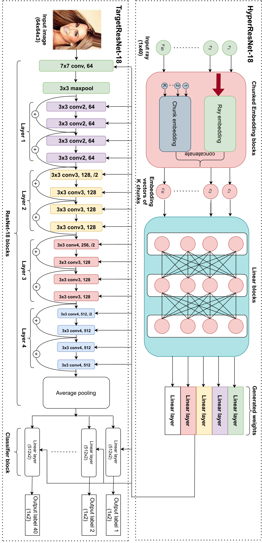
Continually investigate Controllable Pareto Front Learning in large scale problem, we solve the problem of recognizing 40 facial attributes (40 tasks) in 200K face images on CelebA dataset (Liu et al. 2015) using a big Target network: Resnet18 (11M parameters) of (He et al. 2016). Due to very high dimensional scale (40 dimension), we sample randomly 1000 testing preference rays and evaluate methods by mA, Pre, Recall, and F1 score in Table 7. Additional details about this experiment is available at Appendix and https://api.wandb.ai/report/tuantran23012000/xn2gxdwu.

7.4 Computational Analysis

Experiments on MOO problems restated the efficacy of exact mapping in our framework. The MED scores in Table 1–3 are relatively small, indicating that the truth optimal solutions and the predictions of Controllable Pareto Front Learning methods are almost equivalent, particularly the Utility function, the novel scalarization of Pareto Hypernetwork. In the meanwhile, as shown in Figure 2(a) and Figure 2(c), although PHN-EPO and PHN-Cheby predictions are virtually identical, their essences are different. To solve the problem, EPO need to solve a linear programming every iteration to guarantee the generated solutions lie along the inverse preference vectors $\mathbf{r}^{-1}$ , while the attribute is the nature of Chebyshev function. That is the reason why PHN-EPO takes many training time, especially on CelebA dataset (the MTL problem with 40 tasks).

Table 8: Inference time on Multi-MNIST, Multi-Fashion, and Multi-Fashion+MNIST datasets by a random reference vector.

		Multi-MNIST	Multi-Fashion	Fashion-MNIST
Method	params	Infer-time (min.)	Infer-time (min.)	Infer-time (min.)
LS	32K	3.5	3.3	3.2
EPO	35K	8.1	8.3	8.2
PMTL	33K	11.3	11.7	11.4
PHN-EPO	3.3M	0.017	0.018	0.018
PHN-LS	3.3M	0.022	0.019	0.018
PHN-Cheby (ours)	3.3M	0.016	0.018	0.019
PHN-Utility (ours)	3.3M	0.019	0.017	0.017

The MTL experiments demonstrated the superior inference of hypernetwork-based methods. Table 8 shows the inference time of the Controllable Pareto Front Learning framework, which maps a preference vector to a point on the Pareto Front corresponding. We define the inference time as the duration from the input of the reference vector until the algorithm output the Pareto optimal solution. Our proposed framework is faster 100 than prior methods such as LS, EPO, and PMTL, which must train a CNN model to obtain a solution corresponding to a preference vector. The main reason is that the framework is pre-trained (offline learning) with extended priority vector data instead of directly calculating it to find the Pareto optimal solution from a corresponding reference vector (online learning).

8 Conclusion and Future Work

In this paper, we have proved the convergence of Completed Scalarization Functions for convex MOO problem in order to develop Controllable Pareto Front Learning, a brilliant framework to approximate the entire Pareto front, with a comprehensive mathematical explanation of why Hypernetwork may give a precise mapping between a preference vector and the corresponding Pareto optimal solution. However, in some cases, decision-makers cannot choose an explicit preference vector, and only express relative importance between objectives. We provide further discussions about this situation in the Appendix A. Controllable Pareto Front Learning offers significant promise for real-world Multi-Objective Systems that require real-time control and can integrate with the newest research in Machine Learning such as Graph Neural Networks, Knowledge Graph (Pham et al. 2021; Pham et al. 2022). Future work might relate to the provision of the Scalarization functions on the premise that they are monotonically increasing and pseudoconvex. In addition, we also provide the option to expand the class of the Scalarization function, which can be found in Appendix C.3.

Acknowledgments

This work was supported by Vietnam Ministry of Education and Training under Grant number [B2023-BKA-07].

Appendix A PREFERENCE ORDER CONSTRAINTS

In many cases, decision-makers are unable to provide an exact preference vector and instead offer a general description of preference-order constraints, often in the form of a rank list indicating the relative importance of different tasks. Notably, according to Abdolshah et al. 2019, preference-order constraints are closely linked to the definition of Pareto Stationary points (Definition 2.4), which satisfy the stationary equation where the weighted sum of gradients equals zero. Specifically, a point satisfies the condition of task 1 being more important than task 0 if the weight assigned to task 1 in the Pareto stationary equation is greater than the weight assigned to task 0. Consequently, this constraint creates a subset within the Pareto set, as depicted by the red region in figure 3.

Figure 3: The weight

d_{1},d_{2}

of stationary equation representing that objective 1 is more important than objective 2

On the other hand, our framework is designed to discover the entire Pareto set. Therefore, after optimizing the hypernetwork using the Equation (PHN-CSF) described in the paper, we can identify the subset that aligns with the preference-order constraints specified by the decision-maker. As a result, our model remains valid and capable of accommodating these constraints effectively.

Appendix B EXPERIMENTAL DETAILS

B.1 MOO problems

The experiments MOO were implemented on a computer with Intel(R) Core(TM) i7-10700, 64-bit CPU $@2.90$ GHz, and RAM 16GB.

Example 7.1: In this example, we use a multi-layer perceptron (MLP) as the Hypernetwork model, which has the following structure:

	$\displaystyle h(\mathbf{r},\phi):$	$\displaystyle\textbf{Input}(\mathbf{r})\to\textbf{Linear}(2,100)\to\textbf{ReLU}$
		$\displaystyle\to\textbf{Linear}(100,100)\to\textbf{ReLU}$
		$\displaystyle\to\textbf{Linear}(100,1)\to\textbf{Sigmoid}\to\textbf{Output}(\mathbf{x}_{\mathbf{r}}).$

We utilize Hypernetwork to generate an approximate efficient solution from a reference vector created by Dirichlet distribution with $\alpha=0.6$ . We trained all completion functions using an Adam optimizer (Kingma and Ba 2014) with a learning rate of $1e-3$ and $10000$ iterations. In the test phase, we sampled $[5,10,50,100,300,600]$ preference vectors based on the method of (Das and Dennis 1997). Besides, we also illustrated target points and predicted points from the pre-trained Hypernetwork in Figure 2 (top).

Example 7.2: The structure of Hypernetwork has the following structure:

	$\displaystyle h(\mathbf{r},\phi):$	$\displaystyle\textbf{Input}(\mathbf{r})\to\textbf{Linear}(2,100)\to\textbf{ReLU}$
		$\displaystyle\to\textbf{Linear}(100,100)\to\textbf{ReLU}$
		$\displaystyle\to\textbf{Linear}(100,100)\to\textbf{ReLU}$
		$\displaystyle\to\textbf{Linear}(100,2)\to\textbf{Output}(\mathbf{x}_{\mathbf{r}}).$

Unlike Example 7.1, in this example, we did not have the Sigmoid layer before the Output layer but instead direct $\mathbf{x}_{\mathbf{r}}$ from the last Linear layer. We use five preference vectors (0.2, 0.8), (0.4, 0.6),(0.3,0.7), (0.5,0.5, (0.7,0.3), (0.6,0.4), (0.9,0.1) to visualize minimized and valued objectives predicted from the Hypernetwork in Figure 2 (middle).

Example 7.3: To satisfy the equation constraint, in the last layer, we pass the output of the previous layer via a non-linear layer (Square Root Layer), the following structure:

	$\displaystyle h(\mathbf{r},\phi):$	$\displaystyle\textbf{Input}(\mathbf{r})\to\textbf{Linear}(3,100)\to\textbf{ReLU}$
		$\displaystyle\to\textbf{Linear}(100,100)\to\textbf{ReLU}$
		$\displaystyle\to\textbf{Linear}(100,100)\to\textbf{ReLU}$
		$\displaystyle\to\textbf{Linear}(100,100)\to\textbf{ReLU}$
		$\displaystyle\to\textbf{Linear}(100,3)\to\textbf{Softmax}$
		$\displaystyle\to\textbf{Sqrt}\to\textbf{Output}(\mathbf{x}_{\mathbf{r}}).$

Base on (Das 2000), we define subregions $\Omega_{i}$ by points $u=(u_{1},\dots,u_{p})\in U\subset\mathcal{P}$ such that:

\displaystyle u_{1}\in\{0,\delta,2\delta,\dots,...,1\}\text{ s.t }\frac{1}{\delta}=k\in\mathbb{N}^{*}

If $1<j<m-1$ , $n_{i}=\frac{\delta}{u_{i}},1\leq i<j-1$ , we have:

\displaystyle u_{j}\in\{0,\delta,\dots,(p-\sum_{i=1}^{j-1}n_{i})\delta\}\text{, }u_{m}=1-\sum_{j=1}^{m-1}u_{j}

We used the Delaunay triangulation algorithm (Edelsbrunner and Seidel 1985) for generating preference vectors in 3D space. Then we conduct experiments on those vectors and illustrate results in Figure 2 by setting $k=10$ . Then, the number of points $u\in U$ in the space $\mathcal{P}$ is $\Big(^{m+k-1}_{k}\Big)=66$ . However, the Pareto optimal solution corresponds to the intersection of the preference vector $\mathbf{r}^{-1}$ and the Pareto front for PHN-Cheby and PHN-EPO. Because of this, to avoid choosing vectors with coordinate values of 0, we only use vectors with different coordinates better than 0.16. Ten preference vectors in the set of vectors will correspond to the value $k=10$ .

B.2 Multi-task Learning problems

When experimenting, we set up MTL problems on a Linux server with Intel Xeon(R), Silver 4216 64-bit CPU $@2.10$ GHz, RAM 64GB, and VGA NVIDIA Tesla T4 16GB.

Image Classification: We use Multi-LeNet (Sener and Koltun 2018) to train Hypernetwork. The network’s architecture is illustrated in Figure 11. In this experiments, we use Cross-Entropy loss, an Adam optimizer with a batch size of 256 and a learning rate of $1e-4$ over 150 epochs. The validation set is then used to decide the optimal Hypervolume for each approach. We evaluate the Hypernetwork using 25 random preference vectors. The results on the test set are visualized Figure 7.

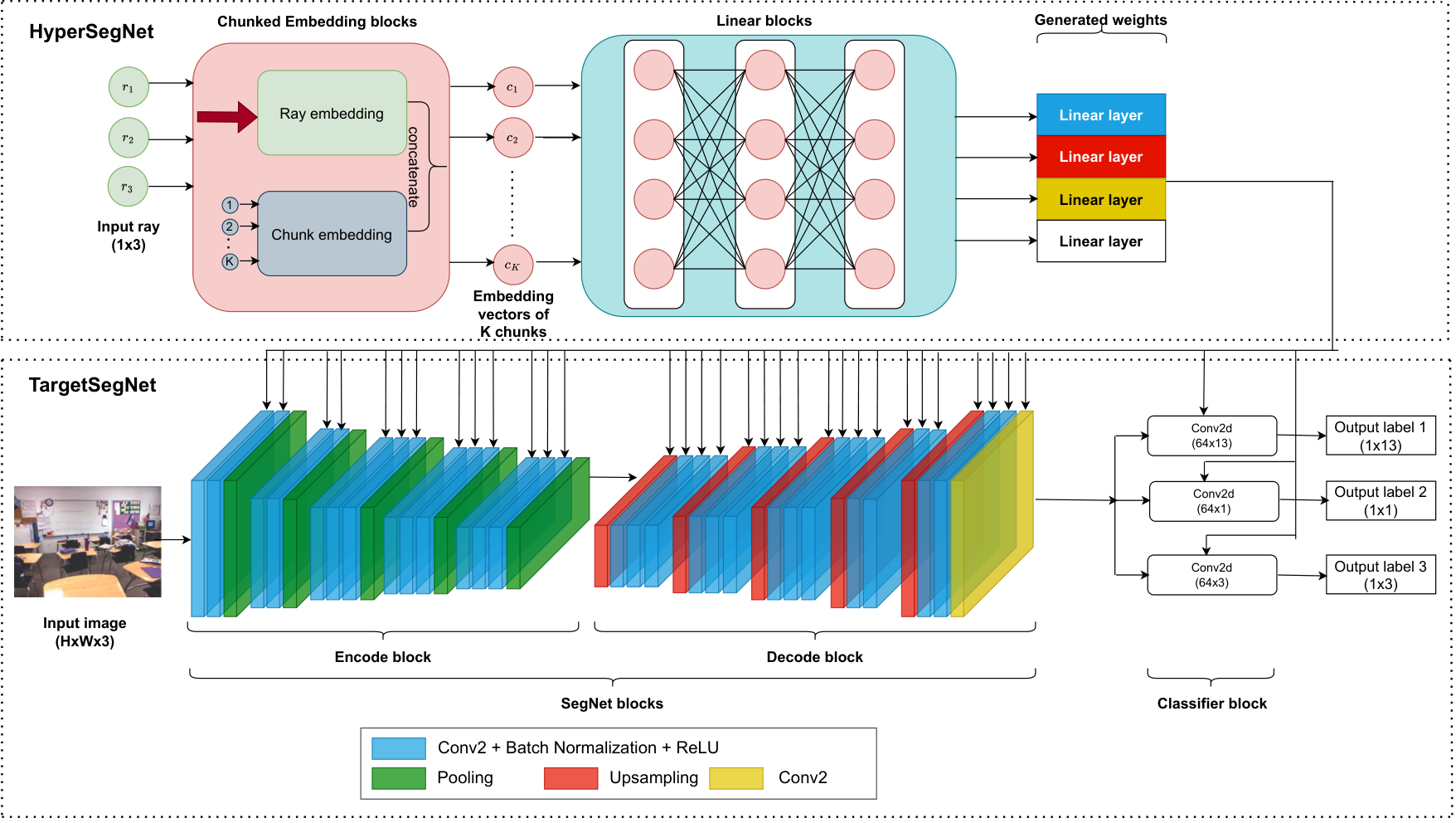
Scene Understanding: When it comes to the Target network, we make use of a SegNet architecture (Badrinarayanan et al. 2017). Each method is trained for 100 epochs using the Adam optimizer with the following parameters: an initial learning rate of $1e-4$ , $\alpha=0.2$ , and a batch size of 14. With 795 train images, 436 validation images, and 218 test images, using the (Das 2000) algorithm, 23 evaluated and 28 tested rays were created to achieve the greatest possible hypervolume on the validation set. We use the chunking technique (Ha et al. 2016; Von Oswald et al. 2019) to generate and reduce the number of parameters for the Hyper-SegNet architecture as Figure 12.

Multi-Output Regression: The target network is Multi-Layer Perceptron which has 21 input variables, 3 layers with 128 units, activation ReLU, and a fully-connected layer. We parameterize $h(\mathbf{r},\phi)$ on Hypernetwork using a feed-forward network with a range of outputs. Each output generates a unique weight tensor for the target network. To construct shared features, the input $\mathbf{r}$ is first mapped to the 100-dimensional space using a multi-layer perceptron network. These features are passed across fully connected levels in the target network to produce a weight matrix for each layer. Using an Adam optimizer with a learning rate of $1e-3$ and a batch size of 512, we train all algorithms. We multiply the learning rate by $\sqrt{2}$ if the algorithm fails to update the best model for 40 consecutive epochs. $\alpha$ was set to $0.2$ . By dividing them by the quantile of 0.9, we normalize the output variables.

Multi-Label Classification: We conduct an experiment to the CelebA dataset, which includes more than $200000$ face images annotated with 40 binary labels, we use a HyperResnet-18 to generate the weight of layers for TargetResnet-18 as Figure 13. In this experiment, we split the dataset into 162770 train images with sizes of $64\times 64$ , 19867 valid images, and 19962 test images. We train using 100 epochs, a $5e-4$ learning rate, and the best weight is stored by evaluating five preference vectors with a Mean Accuracy score. Besides, we report a performance comparison of methods on the CelebA dataset in Table 7. Performance on four metrics, Mean Accuracy, Precision, Recall, and F1 score, are evaluated by 25 random preference vectors.

B.3 Hypervolume Reference Point

The $m$ -dimensional reference point serves as a crucial hyperparameter in the hypervolume indicator. In scenarios where the true Pareto front is unknown, and no specific objectives are prioritized, the reference point should be set equally on all coordinates. Fortunately, selecting an appropriate reference point that facilitates well-spread predictions to approximate the entire Pareto front is not a complex task. Often, choosing a reference point with coordinates higher than those obtained from a random initialization of network losses proves to be sufficient for evaluating outcomes.

Appendix C ADDITIONAL EXPERIMENTS

C.1 Approximation Pareto front.

According to Section 4, the Pareto front may include an endless number of optimum values with varying trade-offs. In addition, the Pareto optimal solutions lack a definitive ranking. A Pareto Front Learning model for the Completed Scalarization function should be capable of approximating the whole Pareto Front and should make it simple to investigate any trade-off. In the training procedure, we employ Dirichlet distribution to produce preference vectors (rays) with $\alpha=0.2$ , the number of rays having the effect of approximating the complete Pareto set in order to construct the entire Pareto front. As Figure 8, Figure 9, and Figure 10, when there are a more significant number of rays used for learning, the Pareto front becomes more covered.

C.2 Gradient Explainer Hypernetwork

Figure 14 and Figure 15 display the influence of preference vectors on Hypernetwork’ prediction of the left (right) digit in the Multi-MNIST dataset. For this purpose, we additionally use the SHAP framework (Lundberg and Lee 2017). When the prediction of a class is a higher probability, the pixels will be red, and when it is lower, the pixels will be blue.

In addition, we apply the GradientExplainer to the CelebA dataset to explain the model’s behavior as it is being trained. As seen in Figure 16, the probability densities of the red entry points are distributed most heavily in the areas of the face that contain the characteristics whose probability we want to predict.

C.3 Design Scalarization Functions

From Proposition 5.21 of (Dinh The 2005), scalarization function $s$ be a monotonically increasing function, then every optimal solution of Problem (CP) be an efficient solution to Problem (MOP). However, it can not be a completed scalarization function, hence, we experiment the extended Scalarization functions based on theory of (Mahapatra and Rajan 2021; Kamani et al. 2021; Chugh 2020).

Kullback–Leibler divergence function. KL-divergence is a distance measurement function to minimize distance of two distributions:

\displaystyle s_{KL}(\mathcal{F},\mathbf{r})=\sum_{i=1}^{m}\sigma_{i}(\mathcal{F},\mathbf{r})\log\left(m\sigma_{i}(\mathcal{F},\mathbf{r})\right),

(KL)

where $\sigma_{i}(\mathcal{F},\mathbf{r})=\dfrac{e^{r_{i}f_{i}}}{\sum_{i=1}^{m}e^{r_{i}f_{i}}},\forall i=1,\dots,m$ . $s_{KL}$ is a strongly convex on $Y$ .

Cauchy–Schwarz function. Cauchy is a proportionality measuring function:

\displaystyle s_{Cauchy}\left(\mathcal{F},\mathbf{r}^{-1}\right)=1-\dfrac{\left<\mathcal{F},\mathbf{r}^{-1}\right>^{2}}{\|\mathcal{F}\|^{2}\|\mathbf{r}^{-1}\|^{2}},

(Cauchy)

where $s_{Cauchy}$ was implied by the Cauchy-Schwarz inequality pertaining to non-zero vectors $\mathcal{F},\mathbf{r}^{-1}\in\mathbb{R}^{m}_{+}$ .

Cosine-Similarity function. Cosine is a form of the Utility function, which has the following formula:

\displaystyle s_{Cosine}\left(\mathcal{F},\mathbf{r}\right)=-\dfrac{\left<\mathcal{F},\mathbf{r}\right>}{\|\mathcal{F}\|\|\mathbf{r}\|}.

(Cosine)

Log function. Log is also a form of the Utility function:

\displaystyle s_{Log}\left(\mathcal{F},\mathbf{r}\right)=\sum_{i=1}^{m}r_{i}\log{(f_{i}+1)}.

(Log)

Prod function. Prod is weighted product function, which was also called as product of powers:

\displaystyle s_{Prod}\left(\mathcal{F},\mathbf{r}\right)=\displaystyle\prod_{i=1}^{m}\left((f_{i}+1)^{r_{i}}\right).

(Prod)

AC function. AC is augmented chebyshev function, which was added by LS function:

\displaystyle s_{AC}\left(\mathcal{F},\mathbf{r}\right)=\underset{i=1,\dots,m}{\max}\{r_{i}f_{i}\}+\rho\sum_{i=1}^{m}r_{i}f_{i},

(AC)

where $\rho>0$ .

MC function. MC is modified chebyshev function, which has form as:

\displaystyle s_{MC}\left(\mathcal{F},\mathbf{r}\right)=\underset{i=1,\dots,m}{\max}\{r_{i}f_{i}+\rho\sum_{i=1}^{m}r_{i}f_{i}\},

(MC)

where $\rho>0$ .

HVI function. HVI is hypervolume indicator function, which was considered by (Hoang et al. 2022), has the following formula:

\displaystyle s_{HVI}\left(\mathcal{F},\mathbf{r}\right)=-HV(\mathcal{F},\mathbf{ref})+\rho s_{Cosine}\left(\mathcal{F},\mathbf{r}\right),

(HVI)

where $s_{Cosine}\left(\mathcal{F},\mathbf{r}\right)=-\dfrac{\left<\mathcal{F},\mathbf{r}\right>}{\|\mathcal{F}\|\|\mathbf{r}\|}$ , $\mathbf{ref}$ is a reference point, and $\rho>0$ .

We simple to verify that all of the consideration Scalarization functions satisfy monotonically increasing assumption on $Y$ , the testing procedure yielded outcomes that give us optimism in Table 9.

Table 9: We sample

1000

preference vectors and evaluate

50

random vectors follow-up time of 30 executions.

	Example 7.1	Example 7.2	Example 7.3
Method	MED $\Downarrow$	MED $\Downarrow$	MED $\Downarrow$
PHN-EPO	$0.0088\pm 0.0006$	$0.0017\pm 0.0002$	$0.0808\pm 0.0052$
PHN-LS	$0.0042\pm 0.0008$	$0.0017\pm 0.0002$	$0.0494\pm 0.0043$
PHN-Cheby	$0.0084\pm 0.0005$	$0.0019\pm 0.0002$	$0.0395\pm 0.0036$
PHN-Utility ( $ub=2.01$ )	$0.0025\pm 0.0003$	$\bf 0.0013\pm 0.0001$	$\bf 0.0201\pm 0.0022$
PHN-KL	$0.0052\pm 0.0003$	$0.0124\pm 0.0002$	$0.0373\pm 0.0039$
PHN-Cauchy	$0.0037\pm 0.0003$	$0.0232\pm 0.0007$	$0.0642\pm 0.0025$
PHN-Cosine	$0.0051\pm 0.0007$	$0.0259\pm 0.0017$	$0.0396\pm 0.0028$
PHN-Log	$0.0321\pm 0.0343$	$0.0031\pm 0.0002$	$0.0225\pm 0.0035$
PHN-Prod	$0.0432\pm 0.0412$	$0.0084\pm 0.0008$	$0.0385\pm 0.0042$
PHN-AC ( $\rho=0.0001$ )	$0.0052\pm 0.0005$	$0.0091\pm 0.0014$	$0.0222\pm 0.0039$
PHN-MC ( $\rho=0.0001$ )	$0.0078\pm 0.0008$	$0.0136\pm 0.0008$	$0.0267\pm 0.0044$
PHN-HVI ( $\rho=100,heads=8$ )	$\bf 0.0017\pm\bf 0.0002$	$0.0092\pm 0.0011$	$0.0303\pm 0.0087$

C.4 Non-Convex MOO Problems

We experiment with the additional test problems, including ZDT1-2 (Zitzler et al. 2000), and DTLZ2 (Deb et al. 2002). Dimensions and attributes for those test problems were illustrated in Table 10. We use Algorithm 2 to train Hypernetwork the following structure:

	$\displaystyle h(\mathbf{r},\phi):$	$\displaystyle\textbf{Input}(\mathbf{r})\to\textbf{Linear}(m,100)\to\textbf{ReLU}$
		$\displaystyle\to\textbf{Linear}(100,100)\to\textbf{ReLU}$
		$\displaystyle\to\textbf{Linear}(100,n)\to\textbf{Sigmoid}\to\textbf{Output}(\mathbf{x}_{\mathbf{r}}),$

with $100000$ iterations, $\alpha=0.6$ , 0.001 learning rate, and Adam optimizer. With the convex Pareto-optimal set in the test problem ZDT1, scalarization functions make a discrepancy between the predicted and optimal solutions. As shown in Figure 5, linear scalarization and utility functions perform poorly with the non-convex Pareto-optimal set in the test problems ZDT2 and DTLZ2.

Table 10: Dimensions and attributes for the MOO problems.

Problem	n	m	Objective function	Pareto-optimal
ex7.1	1	2	convex	convex
ex7.2	2	2	convex	convex
ex7.3	3	3	convex	convex
ZDT1	30	2	non-convex	convex
ZDT2	30	2	non-convex	non-convex
DTLZ2	10	3	non-convex	non-convex

Our experimental results reveal that the hypernet falls short in accurately approximating non-convex functions (ZDT1, ZDT2, and DTLZ2). Specifically, PHN-LS and PHN-Utility encounter challenges in handling Concave-Shape Pareto Fronts, leading to poor performance. Nevertheless, it’s worth noting that PHN-Cheby and PHN-EPO continue to perform well in these scenarios.

C.5 Controllable Pareto Front Learning with no shared optimized variables

Consider the problem when the two objectives in a synthetic scenario are independent of each other, i.e. the entire Pareto front collapses to one single point:

	$\displaystyle\min$	$\displaystyle\left\{x_{1},x_{2}\right\}$
	s.t.	$\displaystyle 0\leq x_{1},x_{2}\leq 1.$

We use Hypernetwork the following structure:

	$\displaystyle h(\mathbf{r},\phi):$	$\displaystyle\textbf{Input}(\mathbf{r})\to\textbf{Linear}(m,100)\to\textbf{ReLU}$
		$\displaystyle\to\textbf{Linear}(100,100)\to\textbf{ReLU}$
		$\displaystyle\to\textbf{Linear}(100,n)\to\textbf{Sigmoid}\to\textbf{Output}(\mathbf{x}_{\mathbf{r}}),$

If the functions $f_{1}$ and $f_{2}$ are independent, meaning they do not share optimized variables, specific ML Pareto solvers like MOO-MTL (Sener and Koltun 2018), PMTL (Lin et al. 2020), or EPO (Mahapatra and Rajan 2021) encounter issues as they rely on a common descent direction for shared variables. Besides, those algorithms did not perform the projection on the constraint space at each iteration. Consequently, these solvers return NaN, a value outside the feasible set or crash in this example. In contrast, our framework, Controllable PFL, operates by optimizing the parameters of the hypernetwork rather than the shared variables, and utilizes the constraint function, such as the Sigmoid function, to control output. This fundamental distinction allows our framework to perform effectively even in such unique scenarios. Interestingly, PHN-EPO also does not fail because it directly applies the EPO solver to the parameters of the hypernetwork.

Experiment results of this special example are shown in the Figure 4 and 5. Our framework Controllable PFL is still work well, and return the optimal value $(0,0)$ for all preference vectors.

(a) PHN-EPO

(b) PHN-LS

(d) PHN-Utility

Figure 6: Output of Controllable Pareto Front Learning method in ZDT1 (top), ZDT2 (middle), and DTLZ2 (bottom). The black dashed line represents the

\mathbf{r}^{-1}

ray in Figures (a) and Figures (c). The red and black points are the target and predicted points respectively.

Figure 7: Pareto front generated by methods.

(a) 50 rays training.

(b) 300 rays training.

Figure 8: Utilize (LS) for learning Hypernetwork to approximate Pareto Front of Example 7.1.

(a) 50 rays training.

(b) 100 rays training.

Figure 9: Utilize (LS) for learning Hypernetwork to approximate Pareto Front of Example 7.2.

References

Abdolshah et al. (2019) Abdolshah, M., Shilton, A., Rana, S., Gupta, S., Venkatesh, S., 2019. Multi-objective bayesian optimisation with preferences over objectives. Advances in neural information processing systems 32.
Ánh et al. (2022) Ánh, H.T., Tuan, T.A., Long, H.P., Hà, L.H., Thang, T.N., 2022. Multi deep learning model for building footprint extraction from high resolution remote sensing image, in: Intelligent Systems and Networks. Springer, pp. 246–252.
Avriel et al. (2010) Avriel, M., Diewert, W.E., Schaible, S., Zang, I., 2010. Generalized concavity. SIAM.
Badrinarayanan et al. (2017) Badrinarayanan, V., Kendall, A., Cipolla, R., 2017. Segnet: A deep convolutional encoder-decoder architecture for image segmentation. IEEE transactions on pattern analysis and machine intelligence 39, 2481–2495.
Bauschke et al. (2011) Bauschke, H.H., Combettes, P.L., et al., 2011. Convex analysis and monotone operator theory in Hilbert spaces. volume 408. Springer.
Benson (1998) Benson, H.P., 1998. An outer approximation algorithm for generating all efficient extreme points in the outcome set of a multiple objective linear programming problem. Journal of Global Optimization 13, 1–24.
Bian et al. (2018) Bian, W., Ma, L., Qin, S., Xue, X., 2018. Neural network for nonsmooth pseudoconvex optimization with general convex constraints. Neural Networks 101, 1–14.
Biewald (2020) Biewald, L., 2020. Experiment tracking with weights and biases. URL: https://www.wandb.com/. software available from wandb.com.
Bilen and Vedaldi (2016) Bilen, H., Vedaldi, A., 2016. Integrated perception with recurrent multi-task neural networks. Advances in neural information processing systems 29.
Binh and Korn (1997) Binh, T.T., Korn, U., 1997. Mobes: A multiobjective evolution strategy for constrained optimization problems, in: The third international conference on genetic algorithms (Mendel 97), p. 27.
Boyd et al. (2004) Boyd, S., Boyd, S.P., Vandenberghe, L., 2004. Convex optimization. Cambridge university press.
Cao et al. (2019) Cao, X., Jia, S., Luo, Y., Yuan, X., Qi, Z., Yu, K.T., 2019. Multi-objective optimization method for enhancing chemical reaction process. Chemical Engineering Science 195, 494–506.
Chauhan et al. (2023) Chauhan, V.K., Zhou, J., Lu, P., Molaei, S., Clifton, D.A., 2023. A brief review of hypernetworks in deep learning. arXiv:2306.06955.
Chen et al. (2018) Chen, Z., Badrinarayanan, V., Lee, C.Y., Rabinovich, A., 2018. Gradnorm: Gradient normalization for adaptive loss balancing in deep multitask networks, in: International conference on machine learning, PMLR. pp. 794–803.
Chugh (2020) Chugh, T., 2020. Scalarizing functions in bayesian multiobjective optimization, in: 2020 IEEE Congress on Evolutionary Computation (CEC), IEEE. pp. 1–8.
Cobb and Douglas (1928) Cobb, C.W., Douglas, P.H., 1928. A theory of production. The American Economic Review 18, 139–165. URL: http://www.jstor.org/stable/1811556.
Cybenko (1989) Cybenko, G., 1989. Approximation by superpositions of a sigmoidal function. Mathematics of control, signals and systems 2, 303–314.
Das and Dennis (1997) Das, I., Dennis, J.E., 1997. A closer look at drawbacks of minimizing weighted sums of objectives for pareto set generation in multicriteria optimization problems. Structural optimization 14, 63–69.
Das (2000) Das, Indraneel a nd Dennis, J., 2000. Normal-boundary intersection: A new method for generating the pareto surface in nonlinear multicriteria optimization problems. SIAM Journal on Optimization 8. doi:10.1137/S1052623496307510.
Deb et al. (2002) Deb, K., Thiele, L., Laumanns, M., Zitzler, E., 2002. Scalable multi-objective optimization test problems, in: Proceedings of the 2002 Congress on Evolutionary Computation. CEC’02 (Cat. No. 02TH8600), IEEE. pp. 825–830.
Dennis Jr and Schnabel (1996) Dennis Jr, J.E., Schnabel, R.B., 1996. Numerical methods for unconstrained optimization and nonlinear equations. SIAM.
Désidéri (2012) Désidéri, J.A., 2012. Multiple-gradient descent algorithm (mgda) for multiobjective optimization. Comptes Rendus Mathematique 350, 313–318.
Dilip et al. (2018) Dilip, L., Bhesdadiya, R., Trivedi, I., Jangir, P., 2018. Optimal power flow problem solution using multi-objective grey wolf optimizer algorithm, in: Intelligent Communication and Computational Technologies: Proceedings of Internet of Things for Technological Development, IoT4TD 2017, Springer. pp. 191–201.
Dinh The (2005) Dinh The, L., 2005. Generalized convexity in vector optimization. Handbook of generalized convexity and generalized monotonicity , 195–236.
Dong et al. (2015) Dong, D., Wu, H., He, W., Yu, D., Wang, H., 2015. Multi-task learning for multiple language translation, in: Proceedings of the 53rd Annual Meeting of the Association for Computational Linguistics and the 7th International Joint Conference on Natural Language Processing (Volume 1: Long Papers), pp. 1723–1732.
Edelsbrunner and Seidel (1985) Edelsbrunner, H., Seidel, R., 1985. Voronoi diagrams and arrangements. Discrete & Computational Geometry 1, 25–44.
Galanti and Wolf (2020) Galanti, T., Wolf, L., 2020. On the modularity of hypernetworks. Advances in Neural Information Processing Systems 33, 10409–10419.
Ha et al. (2016) Ha, D., Dai, A., Le, Q.V., 2016. Hypernetworks. URL: https://arxiv.org/abs/1609.09106, doi:10.48550/ARXIV.1609.09106.
Hashimoto et al. (2016) Hashimoto, K., Xiong, C., Tsuruoka, Y., Socher, R., 2016. A joint many-task model: Growing a neural network for multiple nlp tasks. arXiv preprint arXiv:1611.01587 .
He et al. (2016) He, K., Zhang, X., Ren, S., Sun, J., 2016. Deep residual learning for image recognition, in: Proceedings of the IEEE conference on computer vision and pattern recognition, pp. 770–778.
Hoang et al. (2022) Hoang, L.P., Le, D.D., Tran, T.A., Tran, T.N., 2022. Improving pareto front learning via multi-sample hypernetworks. URL: https://arxiv.org/abs/2212.01130, doi:10.48550/ARXIV.2212.01130.
Jangir et al. (2021) Jangir, P., Heidari, A.A., Chen, H., 2021. Elitist non-dominated sorting harris hawks optimization: Framework and developments for multi-objective problems. Expert Systems with Applications 186, 115747.
Kamani et al. (2021) Kamani, M.M., Forsati, R., Wang, J.Z., Mahdavi, M., 2021. Pareto efficient fairness in supervised learning: From extraction to tracing. arXiv preprint arXiv:2104.01634 .
Kendall et al. (2018) Kendall, A., Gal, Y., Cipolla, R., 2018. Multi-task learning using uncertainty to weigh losses for scene geometry and semantics, in: Proceedings of the IEEE conference on computer vision and pattern recognition, pp. 7482–7491.
Kingma and Ba (2014) Kingma, D.P., Ba, J., 2014. Adam: A method for stochastic optimization. arXiv preprint arXiv:1412.6980 .
Lambrinidis and Tsantili-Kakoulidou (2021) Lambrinidis, G., Tsantili-Kakoulidou, A., 2021. Multi-objective optimization methods in novel drug design. Expert Opinion on Drug Discovery 16, 647–658.
Le and Lauw (2021) Le, D.D., Lauw, H., 2021. Efficient retrieval of matrix factorization-based top-k recommendations: A survey of recent approaches. Journal of Artificial Intelligence Research 70, 1441–1479.
Le and Lauw (2020) Le, D.D., Lauw, H.W., 2020. Stochastically robust personalized ranking for lsh recommendation retrieval, in: Proceedings of the AAAI Conference on Artificial Intelligence, pp. 4594–4601.
Li and Yao (2019) Li, M., Yao, X., 2019. Quality evaluation of solution sets in multiobjective optimisation: A survey. ACM Computing Surveys (CSUR) 52, 1–38.
Lin et al. (2020) Lin, X., Yang, Z., Zhang, Q., Kwong, S., 2020. Controllable pareto multi-task learning. arXiv preprint arXiv:2010.06313 .
Lin et al. (2019) Lin, X., Zhen, H.L., Li, Z., Zhang, Q., Kwong, S., 2019. Pareto multi-task learning, in: Thirty-third Conference on Neural Information Processing Systems (NeurIPS), pp. 12037–12047.
Liu et al. (2022) Liu, N., Wang, J., Qin, S., 2022. A one-layer recurrent neural network for nonsmooth pseudoconvex optimization with quasiconvex inequality and affine equality constraints. Neural Networks 147, 1–9.
Liu et al. (2019) Liu, S., Johns, E., Davison, A.J., 2019. End-to-end multi-task learning with attention, in: Proceedings of the IEEE/CVF conference on computer vision and pattern recognition, pp. 1871–1880.
Liu et al. (2015) Liu, Z., Luo, P., Wang, X., Tang, X., 2015. Deep learning face attributes in the wild, in: Proceedings of the IEEE international conference on computer vision, pp. 3730–3738.
Luc (1989) Luc, D.T., 1989. Scalarization and Stability. Springer Berlin Heidelberg, Berlin, Heidelberg. pp. 80–108. URL: https://doi.org/10.1007/978-3-642-50280-4_4, doi:10.1007/978-3-642-50280-4_4.
Lundberg and Lee (2017) Lundberg, S.M., Lee, S.I., 2017. A unified approach to interpreting model predictions. Advances in neural information processing systems 30.
Mahapatra and Rajan (2021) Mahapatra, D., Rajan, V., 2021. Exact pareto optimal search for multi-task learning: Touring the pareto front. arXiv preprint arXiv:2108.00597 .
Mangasarian (1994) Mangasarian, O.L., 1994. Nonlinear programming. SIAM.
Miettinen (2012) Miettinen, K., 2012. Nonlinear multiobjective optimization. volume 12. Springer Science & Business Media.
Misra et al. (2016) Misra, I., Shrivastava, A., Gupta, A., Hebert, M., 2016. Cross-stitch networks for multi-task learning, in: Proceedings of the IEEE conference on computer vision and pattern recognition, pp. 3994–4003.
Momma et al. (2022) Momma, M., Dong, C., Liu, J., 2022. A multi-objective / multi-task learning framework induced by pareto stationarity, in: Chaudhuri, K., Jegelka, S., Song, L., Szepesvari, C., Niu, G., Sabato, S. (Eds.), Proceedings of the 39th International Conference on Machine Learning, PMLR. pp. 15895–15907. URL: https://proceedings.mlr.press/v162/momma22a.html.
Murugan et al. (2009) Murugan, P., Kannan, S., Baskar, S., 2009. Nsga-ii algorithm for multi-objective generation expansion planning problem. Electric power systems research 79, 622–628.
Navon et al. (2020) Navon, A., Shamsian, A., Chechik, G., Fetaya, E., 2020. Learning the pareto front with hypernetworks. arXiv preprint arXiv:2010.04104 .
Nguyen (2014) Nguyen, T.B.K., 2014. Cac phuong phap toi uu: Ly thuyet va thuat toan.
Paszke et al. (2019) Paszke, A., Gross, S., Massa, F., Lerer, A., Bradbury, J., Chanan, G., Killeen, T., Lin, Z., Gimelshein, N., Antiga, L., et al., 2019. Pytorch: An imperative style, high-performance deep learning library. Advances in neural information processing systems 32.
Pham et al. (2021) Pham, H.V., Thanh, D.H., Moore, P., 2021. Hierarchical pooling in graph neural networks to enhance classification performance in large datasets. Sensors 21, 6070.
Pham et al. (2022) Pham, V.H., Nguyen, Q.H., Le, T.T., Nguyen, T.X.D., Phan, T.T.K., 2022. A proposal model using deep learning model integrated with knowledge graph for monitoring human behavior in forest protection. TELKOMNIKA (Telecommunication Computing Electronics and Control) 20, 1276–1287.
Premkumar et al. (2021) Premkumar, M., Jangir, P., Sowmya, R., Elavarasan, R.M., 2021. Many-objective gradient-based optimizer to solve optimal power flow problems: analysis and validations. Engineering Applications of Artificial Intelligence 106, 104479.
Rockafellar (1970) Rockafellar, R.T., 1970. Convex analysis. volume 18. Princeton university press.
Sabour et al. (2017) Sabour, S., Frosst, N., Hinton, G.E., 2017. Dynamic routing between capsules. URL: https://arxiv.org/abs/1710.09829, doi:10.48550/ARXIV.1710.09829.
Sawaragi et al. (1985) Sawaragi, Y., NAKAYAMA, H., TANINO, T., 1985. Theory of multiobjective optimization. Elsevier.
Sener and Koltun (2018) Sener, O., Koltun, V., 2018. Multi-task learning as multi-objective optimization. Advances in neural information processing systems 31.
Silberman et al. (2012) Silberman, N., Hoiem, D., Kohli, P., Fergus, R., 2012. Indoor segmentation and support inference from rgbd images, in: European conference on computer vision, Springer. pp. 746–760.
Thang (2015) Thang, T.N., 2015. Outcome-based branch and bound algorithm for optimization over the efficient set and its application, in: Some Current Advanced Researches on Information and Computer Science in Vietnam: Post-proceedings of The First NAFOSTED Conference on Information and Computer Science, Springer. pp. 31–47.
Thang and Hai (2022) Thang, T.N., Hai, T.N., 2022. Self-adaptive algorithms for quasiconvex programming and applications to machine learning. URL: https://arxiv.org/abs/2212.06379, doi:10.48550/ARXIV.2212.06379.
Thang and Kim (2016) Thang, T.N., Kim, N.T.B., 2016. Outcome space algorithm for generalized multiplicative problems and optimization over the efficient set. JIMO 12, 1417–1433.
Thang et al. (2016) Thang, T.N., Luc, D.T., Kim, N.T.B., 2016. Solving generalized convex multiobjective programming problems by a normal direction method. Optimization 65, 2269–2292.
Thang et al. (2020) Thang, T.N., Solanki, V.K., Dao, T.A., Thi Ngoc Anh, N., Van Hai, P., 2020. A monotonic optimization approach for solving strictly quasiconvex multiobjective programming problems. Journal of Intelligent & Fuzzy Systems 38, 6053–6063.
Vijayakumar (2000) Vijayakumar, S., 2000. The sarcos dataset. http://www.gaussianprocess.org/gpml/data. URL: http://www.gaussianprocess.org/gpml/data, doi:10.48550/ARXIV.1708.07747.
Von Oswald et al. (2019) Von Oswald, J., Henning, C., Sacramento, J., Grewe, B.F., 2019. Continual learning with hypernetworks. arXiv preprint arXiv:1906.00695 .
Vuong and Thang (2023) Vuong, N.D., Thang, T.N., 2023. Optimizing over pareto set of semistrictly quasiconcave vector maximization and application to stochastic portfolio selection. Journal of Industrial and Management Optimization 19, 1999–2019.
Xiao et al. (2017) Xiao, H., Rasul, K., Vollgraf, R., 2017. Fashion-mnist: a novel image dataset for benchmarking machine learning algorithms. arXiv preprint arXiv:1708.07747 .
Xu et al. (2020) Xu, C., Chai, Y., Qin, S., Wang, Z., Feng, J., 2020. A neurodynamic approach to nonsmooth constrained pseudoconvex optimization problem. Neural Networks 124, 180–192.
Zhang and Li (2008) Zhang, Q., Li, H., 2008. Moea/d: A multiobjective evolutionary algorithm based on decomposition. Evolutionary Computation, IEEE Transactions on 11, 712 – 731. doi:10.1109/TEVC.2007.892759.
Zitzler et al. (2000) Zitzler, E., Deb, K., Thiele, L., 2000. Comparison of multiobjective evolutionary algorithms: Empirical results. Evolutionary computation 8, 173–195.
Zitzler and Thiele (1999) Zitzler, E., Thiele, L., 1999. Multiobjective evolutionary algorithms: a comparative case study and the strength pareto approach. IEEE transactions on Evolutionary Computation 3, 257–271.