Disease Severity Regression with Continuous Data Augmentation

As noted in Section 1, we propose csGAN to generate images at real-valued severity levels. Inspired by StarGAN v2[11], csGAN comprises four modules: a mapping network $F$, a generator $G$, a style encoder $E$, and a discriminator $D$, as shown in Fig. 1(a). csGAN uses a style vector $\bm{s}_{y}(\bm{z})$ as a condition to generate images at the level $y$, where $\bm{z}\sim\mathcal{N}(\bm{0},\bm{I})$. A different $\bm{z}$ results in a different style vector $\bm{s}_{y}(\bm{z})$ and finally contributes to having a different generated image at the level $y$. Hereafter, we often denote $\bm{s}_{y}(\bm{z})$ as $\bm{s}_{y}$ for simplicity.

Due to the page limitation, we briefly summarize the roles of four modules $F$, $G$, $E$, and $D$:

• •

  $F$ accepts a random vector $\bm{z}$ and then outputs $L$ style vectors $\bm{s}_{1},\ldots,\bm{s}_{L}$ at once.

• •

  $G$ accepts a real or generated (i.e., fake) image $\bm{x}$ and the condition $\bm{s}_{y}$ and then generates an image $\bm{x}^{\prime}$ at $y$.

• •

  $E$ accepts a real or fake image $\bm{x}$ with its level $y$ and then estimates its style vector while expecting the estimated vector is similar to $\bm{s}_{y}$ input to $G$.

• •

  $D$ is a standard discriminator for real/fake decisions of $\bm{x}$.

Those modules are trained to achieve cycle consistency; a generated image $\bm{x}^{\prime}=G(\bm{x}_{n},\bm{s}_{y})$ for the level $y\neq y_{n}$ needs to satisfy the condition $\bm{x}_{n}\sim G(\bm{x}^{\prime},\bm{s}_{y_{n}})$. (Note that $\bm{x}_{n}$ is a real image at the level $y_{n}$.) By this cycle consistency, we have a level-$y$ version of $\bm{x}_{n}$ and a level-$y_{n}$ version of $\bm{x}^{\prime}$. Consequently, we have images at all $L$ levels, even from a single image at a certain level $y$.

For generating images at real-valued levels, csGAN introduces an additional loss function, called a order loss, for $F$:

where $\tilde{\bm{s}}_{y}(\bm{z})=(\bm{s}_{y-1}(\bm{z})+\bm{s}_{y+1}(\bm{z}))/2$. With the order loss, we expect that the style vectors from the same $\bm{z}$ will have a linear property, that is,

This linear property will allow us to consider a real-valued severity level $y+\epsilon$, where $\epsilon\in(0,1)$. More specifically, we can derive the style vector for the real-valued level $y+\epsilon$ by the linear interpolation,

As shown in Fig. 1 (a), at the test phase, we use $G$ to generate an image at a real-valued severity level $y^{\prime}=y+\epsilon\in[1,L]$. First, $\{\bm{s}_{1}(\bm{z}),\ldots,\bm{s}_{L}(\bm{z})\}$ is obtained by the mapping network $F$ with a $\bm{z}$. Then, for a certain $\epsilon$, $\bm{s}_{y^{\prime}}$ is determined by Eq. (3). Finally, a level-$y^{\prime}$ version of an image $\bm{x}$ is generated by $\bm{x}^{\prime}=G(\bm{x},\bm{s}_{y^{\prime}})$.

As noted in Section 1, the severity level $y^{\prime}$ of the generated data is not very reliable. Especially, since we used a simple linear style vector interpolation of Eq. (3), we cannot guarantee that the generated data of the level $y^{\prime}=y+\epsilon$ has exact visual characteristics as the level $y^{\prime}$. In other words, the level $y^{\prime}$ is not fully reliable as the absolute level.

However, $y^{\prime}$ is still reliable as a relative level; for a pair of real-valued levels $y^{\prime}_{m}$ and $y^{\prime}_{k}$ (where $y^{\prime}_{m}>y^{\prime}_{k}$), the generated images $\bm{x}^{\prime}_{m}$ and $\bm{x}^{\prime}_{k}$ are expected to show the same relative order in their severity levels, that is, $f(\bm{x}^{\prime}_{m})>f(\bm{x}^{\prime}_{k})$. By training the model $f$ to satisfy this relative condition (instead of training $f$ to satisfy $y_{m}^{\prime}\sim f(\bm{x}^{\prime}_{m})$), we can utilize the augmented data by csGAN in an appropriate manner.

Considering the above property of the generated data, we use dataset-disjoint multi-objective optimization scheme to train the regression model $f$, as shown in Fig. 1 (b). Assume we have an original dataset $\Omega=\{(\bm{x}_{n},y_{n})\}$ with manually-annotated discrete severity levels $y_{n}\in\{1,L\}$ and a generated image dataset $\Omega^{\prime}=\{(\bm{x}^{\prime}_{m},y^{\prime}_{m})\}$ at various real-valued levels $y^{\prime}_{m}\in[1,L]$. Then, the CNN-based regression model $f$ is trained with both datasets $\Omega$ and $\Omega^{\prime}$ in different usages. Since $y_{n}$ is reliable as an absolute level, the image $\bm{x}_{n}$ in $\Omega$ are used to train $f$ to satisfy $y_{n}\sim f(\bm{x}_{n})$. Here, we use a mean squared error loss $\sum_{n=1}^{N}(f(\bm{x}_{n})-y_{n})^{2}/N$. On the other hand, since $y^{\prime}_{m}$ is reliable as a relative level, images $\bm{x}^{\prime}_{m}$ and $\bm{x}^{\prime}_{k}$ in $\Omega^{\prime}$ with the relative relationship $y_{m}^{\prime}>y_{k}^{\prime}$ are used to train $f$ to satisfy $f(\bm{x}^{\prime}_{m})>f(\bm{x}^{\prime}_{k})$. Here, we use the loss function of ListNet [12], which is one of the most popular methods for learning-to-rank. These two loss functions are balanced by a hyperparameter, which is optimized by a validation set.

Fig. 2 shows several examples of endoscopic images for each Mayo score. Schroeder et al.[13] categorized the endoscopic findings of UC as follows: Mayo 0 is a normal or inactive disease, Mayo 1 is a mild disease (erythema, decreased vascular pattern, etc.), Mayo 2 is a moderate disease (marked erythema, erosions, etc.), Mayo 3 is a severe disease (spontaneous bleeding, ulceration, etc.).

We performed five-fold cross-validation. The dataset was divided into training, validation, and test sets at 60, 20, and 20%, respectively. The splittings were performed by random patient-disjoint sampling, and the class ratios for each set were maintained. Moreover, random oversampling was used to mitigate class imbalance in the training set.

In addition, as an ablation study of C-DA, we evaluated the classification performance of a method that uses the original images $\Omega$ as $\Omega^{\prime}$ (C-DA w/o GAN). We also performed C-DA under different severity intervals. Specifically, we examined $\epsilon=1,0.5,$ and $0.25$ to generate 4, 7, and 13 images from a single $z$, respectively. We used 250 randomly selected $z$s and thus generated 1,000, 1,750, and 3,250 images for each $\epsilon$. Note that the validation F1 scores were almost saturated at 250 $z$s; this means that ours show faster saturations than the above conventional methods, which need 20,000 images ($>3,250$) to saturate.

Fig. 4 shows the generated images with and without order loss by csGAN. Each image was generated with $\epsilon=0.5$ from an original image at Mayo 0. With the order loss, the severity shifts smoothly between the generated images as the erythema becomes intense, and the semilunar folds gradually disappear as the severity increases. In contrast, without the order loss, the image generated at Mayo 1.5 shows large noises, and the severity is unclear. This observation confirms that the order loss has a stabilization effect of generating images at real-valued levels.

Table 1 shows the classification performance of each method. Baseline and conventional DA methods had similar F1 scores, while C-DA ($\epsilon=0.5$) had a higher F1 score than the three comparison methods. These results indicate that the generated images with real-valued severity levels are more effective than conventional DAs. The following facts also confirm this effect. First, the F1 score of C-DA ($\epsilon=0.5$) was higher than that of C-DA w/o GAN. Second, F1 scores of C-DA ($\epsilon=0.5$) were even higher than that of C-DA ($\epsilon=1$).

On the other hand, the results also show that image generation at $\epsilon=0.25$ is not very effective. As we noted before, the real-valued levels of the generated images are not completely reliable. Therefore, when $\epsilon$ becomes smaller, the difference between the neighboring levels (e.g., 0.25 and 0.5) becomes unreliable even as the relative levels. This fact indicates a limitation in generating images at real-valued levels, and at the same time, it proves the validity of our dataset-disjoint optimization strategy.

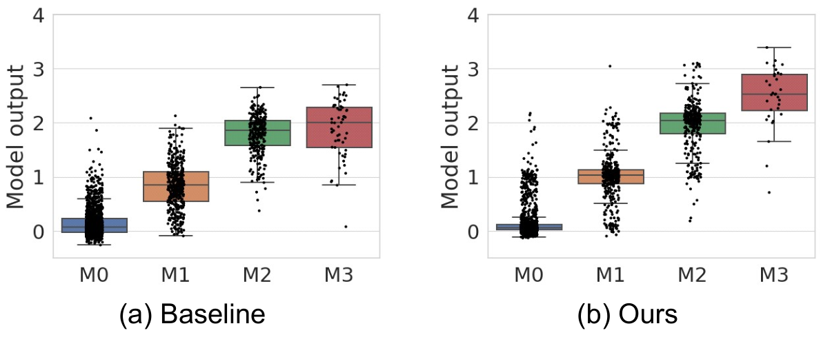
Fig. 4 shows box plots of the model output $f$ for test images of each Mayo score. Here, (a) is the regression (Baseline) and (b) the proposed DA (C-DA($\epsilon=0.5$)). The horizontal and vertical axes correspond to the correct Mayo score and the model outputs, respectively. The overall model outputs of C-DA are a narrower interquartile range for each Mayo score than Baseline. Especially, the overlap between the interquartile ranges of Mayo 2 and Mayo 3 is decreased. Consequently, C-DA had better classification performance, even for minor classes with fewer images.

References

- [1] Andrew Brock, Donahue, Jeff Donahue, and Karen Simonyan, “Large Scale GAN Training for High Fidelity Natural Image Synthesis,” in International Conference on Learning Representations, 2019.
- [2] Han Zhang, Ian Goodfellow, Dimitris Metaxas, and Augustus Odena, “Self-Attention Generative Adversarial Networks,” in Proceedings of the 36th International Conference on Machine Learning, 2019, pp. 7354–7363.
- [3] Augustus Odena, Christopher Olah, and Jonathon Shlens, “Conditional Image Synthesis with Auxiliary Classifier GANs,” in International Conference on Machine Learning, 2017, pp. 2642–2651.
- [4] Jie Gui, Zhenan Sun, Yonggang Wen, Dacheng Tao, and Jieping Ye, “A Review on Generative Adversarial Networks: Algorithms, Theory, and Applications,” IEEE Transactions on Knowledge and Data Engineering, pp. 1–1, 2021.
- [5] Phillip Isola, Jun-Yan Zhu, Tinghui Zhou, and Alexei A Efros, “Image-to-Image Translation with Conditional Adversarial Networks,” in Proceedings of the IEEE Conference on Computer Vision and Pattern Recognition, 2017, pp. 1125–1134.
- [6] Xin Ding, Yongwei Wang, Zuheng Xu, William J Welch, and Z Jane Wang, “CcGAN: Continuous Conditional Generative Adversarial Networks for Image Generation,” in International Conference on Learning Representations, 2021.
- [7] Phillip Chlap, Hang Min, Nym Vandenberg, Jason Dowling, Lois Holloway, and Annette Haworth, “A Review of Medical Image Data Augmentation Techniques for Deep Learning Applications,” Journal of Medical Imaging and Radiation Oncology, vol. 65, no. 5, pp. 545–563, 2021.
- [8] Yunpeng Wang, Lingxiao Zhou, Mingming Wang, Cheng Shao, Lili Shi, Shuyi Yang, Zhiyong Zhang, Mingxiang Feng, Fei Shan, and Lei Liu, “Combination of Generative Adversarial Network and Convolutional Neural Network for Automatic Subcentimeter Pulmonary Adenocarcinoma Classification,” Quantitative Imaging in Medicine and Surgery, vol. 10, no. 6, pp. 1249–1264, 2020.
- [9] Chenjie Ge, Irene Yu-Hua Gu, Asgeir Store Jakola, and Jie Yang, “Enlarged Training Dataset by Pairwise GANs for Molecular-Based Brain Tumor Classification,” IEEE Access, vol. 8, pp. 22560–22570, 2020.
- [10] Hoo-Chang Shin, Neil A Tenenholtz, Jameson K Rogers, Christopher G Schwarz, Matthew L Senjem, Jeffrey L Gunter, Katherine P Andriole, and Mark Michalski, “Medical Image Synthesis for Data Augmentation and Anonymization Using Generative Adversarial Networks,” in International Workshop on Simulation and Synthesis in Medical Imaging, 2018, pp. 1–11.
- [11] Yunjey Choi, Youngjung Uh, Jaejun Yoo, and Jung-Woo Ha, “StarGAN v2: Diverse Image Synthesis for Multiple Domains,” in Proceedings of the IEEE Conference on Computer Vision and Pattern Recognition, 2020, pp. 8188–8197.
- [12] Zhe Cao, Tao Qin, Tie-Yan Liu, Ming-Feng Tsai, and Hang Li, “Learning to Rank: From Pairwise Approach to Listwise Approach,” in Proceedings of the 24th International Conference on Machine Learning, 2007, pp. 129–136.
- [13] Kenneth W Schroeder, William J Tremaine, and Duane M Ilstrup, “Coated Oral 5-Aminosalicylic Acid Therapy for Mildly to Moderately Active Ulcerative Colitis,” New England Journal of Medicine, vol. 317, no. 26, pp. 1625–1629, 1987.
- [14] Gao Huang, Zhuang Liu, Laurens Van Der Maaten, and Kilian Q Weinberger, “Densely Connected Convolutional Networks,” in Proceedings of the IEEE Conference on Computer Vision and Pattern Recognition, 2017, pp. 4700–4708.
- [15] Olga Russakovsky, Jia Deng, Hao Su, Jonathan Krause, Sanjeev Satheesh, Sean Ma, Zhiheng Huang, Andrej Karpathy, Aditya Khosla, Michael Bernstein, Alexander C Berg, and Li Fei-Fei, “ImageNet Large Scale Visual Recognition Challenge,” International Journal of Computer Vision, vol. 115, no. 3, pp. 211–252, 2015.
- [16] Tero Karras, Miika Aittala, Janne Hellsten, Samuli Laine, Jaakko Lehtinen, and Timo Aila, “Training Generative Adversarial Networks with Limited Data,” in Advances in Neural Information Processing Systems, 2020, vol. 33, pp. 12104–12114.