跳到论文正文
W Papers独立论文阅读器 arXiv:2302.12474 论文正文 计算阅读时间 · 0%
引用这篇论文根据当前论文元数据生成,正式投稿前建议核对。


License: arXiv.org perpetual non-exclusive license
arXiv:2302.12474v2 [math.NA] 16 Mar 2023

Convexification for the Viscocity Solution for a Coefficient Inverse Problem for the Radiative Transfer EquationJournal: Inverse Problems

Michael V. Klibanov    Jingzhi Li    Zhipeng Yang Email: mklibanv@uncc.edu Email: li.jz@sustech.edu.cn Email: yangzp@sustech.edu.cn Affiliation:  Department of Mathematics, Southern University of Science and Technology, Shenzhen 518055, P. R. China
Abstract

A Coefficient Inverse Problem for the radiative transport equation is considered. The globally convergent numerical method, the so-called convexification, is developed. For the first time, the viscosity solution is considered for a boundary value problem for the resulting system of two coupled partial differential equations. A Lipschitz stability estimate is proved for this boundary value problem using a Carleman estimate for the Laplace operator. Next, the global convergence analysis is provided via that Carleman estimate. Results of numerical experiments demonstrate a high computational efficiency of this approach.

, ,

March 2023

Keywords: Carleman estimate, viscosity solution, radiative transport equation, coefficient inverse problem, Lipschitz stability estimate, convexification, global convergence, numerical studies.

1 Introduction

The radiative transfer equation (RTE) is commonly used in diffusive optics [17]. In the case of light propagation, RTE governs scattering and absorption of photons when they propagate through a diffusive medium, such as, e.g. turbulent atmosphere and biological medium [17]. RTE is also known as the Boltzmann equation [8, 17].

One of the specific applications is in seeing through a turbulent atmosphere. Another attractive application is in optical molecular imaging (OMI) [35] when some optical markers are attached to specific molecules to detect faulty genes. In the single positron emission computed tomography (SPECT) and in photon emission tomography (PET) markers with the high energy are used. Unlike these, markers of OMI emit a relatively low energy near infrared light. Reconstruction of the attenuation coefficient using measurements of the intensity of the emitted light on parts of the human body should lead to the detection and classification of faulty genes. The latter might result in a better diagnostics.

Coefficient Inverse Problems (CIPs) for PDEs are both nonlinear and ill-posed. These two factors cause major challenges in their numerical solutions. The majority of numerical methods for CIPs is based on a very popular procedure of the minimization of least squares cost functionals.In this regard we refer to e.g. [2, 1, 5, 6, 14, 15, 12, 16]. On the other hand, there is no guarantee of the convexity of these functionals, and this might lead to the existence of multiple local minima and ravines, see, e.g. [32].

To avoid the latter, the convexification method was originally proposed in [22, 18] for the case of CIPs for hyperbolic PDEs. The convexification is a numerical development of the idea of [7], which was originally proposed only for the proofs of global uniqueness theorems for multidimensional CIPs and has been explored by many authors since then, see, e.g. [13, 30, 31] as well as [19] for a survey of results as of 2013, [21] for the most recent result, and the book [25, Chapters 2,3]. In [7] the method of Carleman estimates was introduced in the field of CIPs for the first time. Carleman estimates are also the key to the convexification idea.

In the past few years, members of this research group have been working on various applications of the convexification to numerical solutions of various CIPs, see, e.g. [25] for a summary of results as of 2021. In particular, in two most recent publications they have solved by convexification CIPs for two versions of the RTE. [27, 26]. In both these works one obtains first a boundary value problem (BVP) for a nonlinear PDE of the second order, which does not contain the unknown coefficient. Next, the solution of this BVP is represented via a truncated Fourier series with N>2N>2 terms with respect to a special orthonormal basis. This basis was originally proposed in [20], also, see [25, section 6.2.3]. As a result, one obtains a new BVP for a system of NN coupled nonlinear PDEs of the first order. This BVP is solved via the construction and subsequent minimization of a weighted cost functional. The main element of this functional is the presence of a Carleman Weighted Function (CWF) in it.

The CWF is a function, which is used as a weight in the Carleman estimate for the corresponding PDE operator. The key property of this functional is that it is strictly convex on a convex bounded set of an arbitrary diameter d>0d>0 in an appropriate Hilbert space. Since a smallness condition is not imposed on dd, then it is natural to call that functional globally strictly convex.

The goal of this work is to numerically solve the above mentioned BVP for that nonlinear PDE via perturbing that PDE operator with the viscosity term −ε​Δ,-\varepsilon\Delta, where ε>0\varepsilon>0 is a small number. Then we obtain a BVP for a system of only two coupled nonlinear PDEs of the second order, as opposed to the above case of N>2N>2 PDEs . First, we prove the Lipschitz stability estimate for this BVP using a Carleman estimate for the Laplace operator. Next, we construct a globally strictly convex weighted cost functional for the latter BVP. The key element of this functional is the presence of the Carleman Weight Function in it. This function is involved as the weight in the above mentioned Carleman estimate. The proof of the global strict convexity of that functional is the main part of our global convergence analysis. This analysis ends up with the proof of the global convergence of the gradient descent method of the minimization of that functional. Finally, we conduct exhaustive numerical studies, which demonstrate a good performance of our technique. Previously the viscosity solution of the Hamilton-Jacobi equation was numerically computed in [29] by a different version of the convexification method.

Publications [27, 26] represent the first numerical solutions of CIPs for both RTE [27] and its Riemannian version [26]. Previous numerical results were obtained only for the inverse source problems for RTE in [9, 10, 11, 33] and for RRTE in [24]. However, inverse source problems are linear ones, unlike CIPs. There are also some uniqueness and stability results for CIPs for RTE. Since this paper is not concerned with such results, then we refer here only to a limited number of publications on the latter topic [4, 13, 30, 31].

In section 2 we state both forward and inverse problems. To solve the inverse problem, we obtain in in section 3 a boundary value problem for a 2×22\times 2 system of nonlinear PDEs with viscosity terms. We prove the Lipschitz stability estimate for this boundary value problem in section 4. In section 5 we construct the convexified Tikhonov-like functional and conduct the convergence analysis for it. Numerical experiments are presented in section 6.

2 Statements of Forward and Inverse Problems

For n≥1,n\geq 1, points in ℝn\mathbb{R}^{n} are denoted below as x=(x1,x2,…,xn−1,z)∈ℝn.x=(x_{1},x_{2},...,x_{n-1},z)\in\mathbb{R}^{n}. Let numbers B,a,b,d>0B,a,b,d>0, where

0<a<b.0<a<b. (2.1)

Let Ω⊂ℝn\Omega\subset\mathbb{R}^{n} be a rectangular prism with its boundary ∂Ω=∂1Ω∪∂2Ω∪∂3Ω,\partial\Omega=\partial_{1}\Omega\cup\partial_{2}\Omega\cup\partial_{3}\Omega, where

Ω={x:−B<x1,…,xn−1<B,a<z<b},\displaystyle\Omega=\{x:-B<x_{1},...,x_{n-1}<B,a<z<b\}, (2.2)
∂1Ω={x:−B<x1,…,xn−1<B,z=a},\displaystyle\hskip 5.69046pt\partial_{1}\Omega=\left\{x:-B<x_{1},...,x_{n-1}<B,z=a\right\}, (2.3)
∂2Ω={x:−B<x1,…,xn−1<B,z=b},\displaystyle\hskip 5.69046pt\partial_{2}\Omega=\left\{x\mathbf{:}-B<x_{1},...,x_{n-1}<B,z=b\right\}, (2.4)
∂3Ω={xi=±B,z∈(a,b),i=1,…,n−1}.\displaystyle\hskip 2.84544pt\partial_{3}\Omega=\left\{x_{i}=\pm B,z\in\left(a,b\right),i=1,...,n-1\right\}. (2.5)

Let Φd\Phi_{d} be the line, where the external sources are located,

Φd={xα=(α,0,…,0):α∈[−d,d]}.\Phi_{d}=\{x_{\alpha}=(\alpha,0,...,0):\alpha\in[-d,d]\}. (2.6)

Hence, Φd\Phi_{d} is a part of the x1−x_{1}-axis. By (2.1), (2.2) and (2.6)

Φd∩Ω¯=∅.\Phi_{d}\cap\overline{\Omega}=\varnothing. (2.7)

Let σ>0\sigma>0 be a sufficiently small number. To simplify the presentation, avoid working with singularities. Hence, we consider the following function instead of δ⁡(x)\delta\left(x\right):

fσ​(x)=Cσ​{exp⁡(|x|2σ2−|x|2),|x|<σ,0,|x|≥σ.f_{\sigma}\left(x\right)=C_{\sigma}\left\{\begin{array}[]{c}\exp\left(\frac{\left|x\right|^{2}}{\sigma^{2}-\left|x\right|^{2}}\right),\left|x\right|<\sigma,\\ 0,\left|x\right|\geq\sigma\end{array}\right.. (2.8)

The constant CσC_{\sigma} is chosen here such that

Cσ​∫|x|<σexp⁡(|x|2σ2−|x|2)​𝑑x=1.C_{\sigma}\int\limits_{\left|x\right|<\sigma}\exp\left(\frac{\left|x\right|^{2}}{\sigma^{2}-\left|x\right|^{2}}\right)dx=1. (2.9)

Hence, the function f⁡(x−xα)=f⁡(x1−α,x2,…,xn,z)∈C∞​(ℝn)f\left(x-x_{\alpha}\right)=f\left(x_{1}-\alpha,x_{2},...,x_{n},z\right)\in C^{\infty}\left(\mathbb{R}^{n}\right) can be considered as the source function for the source xα∈Φd.x_{\alpha}\in\Phi_{d}. Let the number σ\sigma be so small that

f⁡(x−xα)=0,∀x∈Ω¯,∀xα∈Φd.f\left(x-x_{\alpha}\right)=0,\forall x\in\overline{\Omega},\forall x_{\alpha}\in\Phi_{d}. (2.10)

Let

B¯=max⁡(B,d).\overline{B}=\max\left(B,d\right). (2.11)

Introduce the domain P⊂ℝnP\subset\mathbb{R}^{n} as well as two of its subdomains Pa+P_{a}^{+},Pa−⊂P,P_{a}^{-}\subset P,

{P={x:|x1|,…,|xn−1|<B¯,z∈(0,b)},Pa+=P∩{z>a},Pa−=P​╲​Pa+.\left\{\begin{array}[]{c}P=\left\{x:\left|x_{1}\right|,...,\left|x_{n-1}\right|<\overline{B},z\in\left(0,b\right)\right\},\\ P_{a}^{+}=P\cap\left\{z>a\right\},\\ P_{a}^{-}=P\diagdown P_{a}^{+}.\end{array}\right. (2.12)

By (2.2), (2.11) and (2.12)

Ω⊆Pa+.\Omega\subseteq P_{a}^{+}. (2.13)

Below

x∈P,α∈(−d,d).x\in P,\ \alpha\in\left(-d,d\right). (2.14)

For two arbitrary points x,y∈ℝnx,y\in\mathbb{R}^{n} denote L⁡(x,y)L\left(x,y\right) the line segment connecting these two points and let d​sds be the element of the euclidean length on L⁡(x,y).L\left(x,y\right). Let ν⁡(x,α)\nu(x\mathbf{,}\alpha) be the unit vector, which is parallel to L⁡(x,xα),L\left(x,x_{\alpha}\right),

ν⁡(x,α)=x−xα|x−xα|,x≠xα.\nu(x\mathbf{,}\alpha)=\frac{x-x_{\alpha}}{\left|x-x_{\alpha}\right|},\ x\neq x_{\alpha}. (2.15)

Let u⁡(x,α)u(x,\alpha) be the steady-state radiance at the point xx generated by the source function f⁡(x−xα).f\left(x-x_{\alpha}\right). The function u⁡(x,α)u(x,\alpha) satisfies the stationary RTE [17]:

ν⁡(x,α)⋅∇xu​(x,α)+a⁡(x)​u​(x,α)=μs(x)∫ΦdG(x,α,β)u(x,β)dβ+f(x−xα),x∈P,xα∈Φd,\left.\begin{array}[]{c}\nu(x\mathbf{,}\alpha)\cdot\nabla_{x}u(x,\alpha)+a\left(x\right)u(x,\alpha)\\ =\mu_{s}(x)\int\limits_{\Phi_{d}}G(x,\alpha,\beta)u(x,\beta)d\beta+f\left(x-x_{\alpha}\right),\ x\in P,x_{\alpha}\in\Phi_{d},\end{array}\right. (2.16)

where “⋅\cdot” denotes the scalar product in ℝn\mathbb{R}^{n}, see (2.14). The kernel G⁡(x,α,β)G(x,\alpha,\beta) of the integral operator in (2.16) satisfies [17, 33]:

G(x,α,β)≥0,x∈P¯;α,β∈[−d,d],\displaystyle G(x,\alpha,\beta)\geq 0,\ x\mathbf{\in}\overline{P};\ \alpha,\beta\in\left[-d,d\right],\ (2.17)
G⁡(x,α,β)∈C1​(P¯×[−d,d]2).\displaystyle\hskip 14.22636ptG(x,\alpha,\beta)\in C^{1}\left(\overline{P}\times\left[-d,d\right]^{2}\right). (2.18)

In (2.16),

a⁡(x)=μa​(x)+μs​(x),a\left(x\right)=\mu_{a}\left(x\right)+\mu_{s}(x), (2.19)

where μa​(x)\mu_{a}\left(x\right) and μs​(x)\mu_{s}(x) are the absorption and scattering coefficients respectively. The function a⁡(x)a\left(x\right) is the attenuation coefficient. We assume that

μa​(x),μs​(x)≥0,μa​(x)=μs​(x)=0,x∈P∖Ω,\displaystyle\mu_{a}\left(x\right),\mu_{s}(x)\geq 0,\mu_{a}\left(x\right)=\mu_{s}(x)=0,\ x\in\mathbb{\ }P\setminus\Omega, (2.20)
μa​(x),μs​(x)∈C⁡(P¯).\displaystyle\hskip 56.9055pt\mu_{a}\left(x\right),\mu_{s}(x)\in C\left(\overline{P}\right). (2.21)

Forward Problem. Let conditions (2.1)-(2.21) hold. Find the function u⁡(x,α)u(x,\alpha) ∈C1​(P¯×[−d,d])\in C^{1}\Big(\overline{P}\times\left[-d,d\right]\Big) satisfying equation (2.16) and the initial condition

u⁡(xα,α)=0​ for ​xα∈Φd.u(x_{\alpha},\alpha)=0\mbox{ for }x_{\alpha}\in\Phi_{d}. (2.22)

Denote

c⁡(x)=exp⁡(∫L⁡(x,xα)a⁡(x⁡(s))​𝑑s).c\left(x\right)=\exp\left(\int_{L(x,x_{\alpha})}a(x\left(s\right))ds\right).

The following existence and uniqueness theorem for the Forward Problem was proven in [27], and a similar theorem was proven in [26] for the Riemannian analog of RTE:

Theorem 2.1 [27]. Assume that conditions (2.1)-( 2.15) and (2.17)-(2.21) hold. Then there exists unique solution u⁡(x,α)∈C1​(P¯×[−d,d])u\left(x,\alpha\right)\in C^{1}\left(\overline{P}\times\left[-d,d\right]\right) of equation (2.16) with the initial condition (2.22), and the function u⁡(x,α)u\left(x,\alpha\right) has the following form for x∈P,α∈(−d,d):x\in P,\alpha\in\left(-d,d\right):

u⁡(x,α)=u0​(x,α)+\displaystyle\hskip 85.35826ptu(x\mathbf{,}\alpha)=u_{0}(x\mathbf{,}\alpha)+ (2.23)
+1c⁡(x,α)∫L⁡(x,xα)c(x(s),α)μs(x(s))(∫ΦdG(x(s),α,β)u(x(s),β)dβ)ds,\displaystyle\hskip-28.45274pt+\frac{1}{c(x\mathbf{,}\alpha)}\int\limits_{L(x,x_{\alpha})}c(x\left(s\right),\alpha)\mu_{s}(x\left(s\right))\left(\int\limits_{\Phi_{d}}G(x\left(s\right),\alpha,\beta)u(x\left(s\right),\beta)d\beta\right)ds,
u0​(x,α)=1c⁡(x,α)​∫L⁡(x,xα)f⁡(x⁡(s)−xα)​𝑑s.\displaystyle\hskip 56.9055ptu_{0}(x\mathbf{,}\alpha)=\frac{1}{c\left(x,\alpha\right)}\int\limits_{L(x,x_{\alpha})}f\left(x\left(s\right)-x_{\alpha}\right)ds. (2.24)

Furthermore, the following inequality holds:

u⁡(x,α)≥m>0​ for ​(x,α)∈P¯a+×[−d,d],m=minP¯a+×[−d,d]⁡u0​(x,α).\displaystyle u\left(x,\alpha\right)\geq m>0\mbox{ for }\left(x,\alpha\right)\in\overline{P}_{a}^{+}\times\left[-d,d\right],\ m=\min_{\overline{P}_{a}^{+}\times\left[-d,d\right]}u_{0}(x\mathbf{,}\alpha). (2.25)

Coefficient Inverse Problem (CIP). Let conditions (2.1 )-(2.21) hold. Let the function u⁡(x,α)∈C1​(G¯×[−d,d])u\left(x,\alpha\right)\in C^{1}\left(\overline{G}\times\left[-d,d\right]\right) be the solution of the Forward Problem as in Theorem 2.1. Assume that the attenuation coefficient a⁡(x)a\left(x\right) in (2.16) is unknown. Assume that the function g⁡(x,α)g\left(x,\alpha\right) is known,

g⁡(x,α)=u⁡(x,α),∀x∈∂Ω,∀α∈(−d,d).g\left(x,\alpha\right)=u\left(x,\alpha\right),\forall x\in\partial\Omega,\forall\alpha\in\left(-d,d\right). (2.26)

Find the function a⁡(x).a\left(x\right).

3 Boundary Value Problem for a 2×22\times 2 System of PDEs With Viscosity Terms

3.1 Preliminaries

It follows from (2.13), (2.14) and (2.25) that we can introduce a new function w⁡(x,α)w(x,\alpha),

w⁡(x,α)=ln⁡u⁡(x,α),(x,α)∈Ω¯×[−d,d].w\left(x,\alpha\right)=\ln u\left(x,\alpha\right),\ \left(x,\alpha\right)\in\overline{\Omega}\times\left[-d,d\right]. (3.1)

Substituting (3.1) in (2.16) and (2.26), we obtain

ν⁡(x,α)⋅∇xw​(x,α)+a⁡(x)\displaystyle\hskip 71.13188pt\nu(x\mathbf{,}\alpha)\cdot\nabla_{x}w(x,\alpha)+a\left(x\right) (3.2)
=e−w⁡(x,α)​μs​(x)​∫ΦdG⁡(x,α,β)​ew⁡(x,β)​𝑑β,x∈Ω,α∈(−d,d),\displaystyle=e^{-w\left(x,\alpha\right)}\mu_{s}(x)\int\limits_{\Phi_{d}}G(x,\alpha,\beta)e^{w\left(x,\beta\right)}d\beta,x\in\Omega,\alpha\in\left(-d,d\right),
w⁡(x,α)∣∂Ω=g1​(x,α)=ln⁡g⁡(x,α).\displaystyle\hskip 56.9055ptw(x,\alpha)\mid_{\partial\Omega}=g_{1}\left(x,\alpha\right)=\ln g\left(x,\alpha\right). (3.3)

Differentiate both sides of (3.2) with respect to α\alpha and use ∂αa⁡(x)≡0.\partial_{\alpha}a\left(x\right)\equiv 0. We obtain an integral differential equation with the derivatives up to the second order,

ν⁡(x,α)⋅∇xwα​(x,α)+∂αν⁡(x,α)⋅∇xw​(x,α)+\displaystyle\hskip 28.45274pt\nu(x\mathbf{,}\alpha)\cdot\nabla_{x}w_{\alpha}(x,\alpha)+\partial_{\alpha}\nu(x\mathbf{,}\alpha)\cdot\nabla_{x}w(x,\alpha)+ (3.4)
+e−w⁡(x,α)wα(x,α)μs(x)∫ΦdG(x,α,β)ew⁡(x,β)dβ−\displaystyle\hskip 22.76228pt+e^{-w\left(x,\alpha\right)}w_{\alpha}\left(x,\alpha\right)\mu_{s}(x)\int\limits_{\Phi_{d}}G(x,\alpha,\beta)e^{w\left(x,\beta\right)}d\beta- (3.5)
−e−w⁡(x,α)μs(x)∫Φd∂αG(x,α,β)ew⁡(x,β)dβ=0,x∈Ω,α∈(−d,d).\displaystyle-e^{-w\left(x,\alpha\right)}\mu_{s}(x)\int\limits_{\Phi_{d}}\partial_{\alpha}G(x,\alpha,\beta)e^{w\left(x,\beta\right)}d\beta=0,x\in\Omega,\alpha\in\left(-d,d\right). (3.6)

By (3.3) the boundary condition for wα​(x,α)w_{\alpha}(x,\alpha) is

wα​(x,α)∣∂Ω=g2​(x,α)=gα​(x,α)g⁡(x,α).w_{\alpha}(x,\alpha)\mid_{\partial\Omega}=g_{2}\left(x,\alpha\right)=\frac{g_{\alpha}\left(x,\alpha\right)}{g\left(x,\alpha\right)}. (3.7)

To work with the viscosity solution, we need to figure out the following boundary conditions, see (2.4):

∂zw⁡(x,α)∣∂2Ω=∂zw⁡(x1,…,xn−1,b,α)=g3​(x,α),\displaystyle\hskip 5.69046pt\partial_{z}w(x,\alpha)\mid_{\partial_{2}\Omega}=\partial_{z}w\left(x_{1},...,x_{n-1},b,\alpha\right)=g_{3}(x,\alpha), (3.8)
∂zwα​(x,α)∣∂2Ω=∂zwα​(x1,…,xn−1,b,α)=g4​(x,α).\displaystyle\partial_{z}w_{\alpha}(x,\alpha)\mid_{\partial_{2}\Omega}=\partial_{z}w_{\alpha}\left(x_{1},...,x_{n-1},b,\alpha\right)=g_{4}(x,\alpha). (3.9)

It follows from (2.6) and (2.15) that ν⁡(x,α)=(ν1​(x,α)CLOSE\nu(x\mathbf{,}\alpha)=(\nu_{1}(x\mathbf{,}\alpha), ν2​(x,α)\nu_{2}(x\mathbf{,}\alpha), ⋯\cdots, νn−1​(x,α)\nu_{n-1}(x\mathbf{,}\alpha), OPENνn​(x,α))\nu_{n}(x\mathbf{,}\alpha)), where

ν1​(x,α)=(x1−α)(x1−α)2+x22+…+xn−12+z2,\displaystyle\hskip 28.45274pt\nu_{1}(x\mathbf{,}\alpha)=\frac{\left(x_{1}-\alpha\right)}{\sqrt{\left(x_{1}-\alpha\right)^{2}+x_{2}^{2}+...+x_{n-1}^{2}+z^{2}}}, (3.10)
νk(x,α)=xk(x1−α)2+x22+…+xn−12+z2,k=2,…,n−1,\displaystyle\nu_{k}(x\mathbf{,}\alpha)=\frac{x_{k}}{\sqrt{\left(x_{1}-\alpha\right)^{2}+x_{2}^{2}+...+x_{n-1}^{2}+z^{2}}},k=2,...,n-1, (3.11)
νn​(x,α)=z(x1−α)2+x22+…+xn−12+z2.\displaystyle\hskip 28.45274pt\nu_{n}(x\mathbf{,}\alpha)=\frac{z}{\sqrt{\left(x_{1}-\alpha\right)^{2}+x_{2}^{2}+...+x_{n-1}^{2}+z^{2}}}. (3.12)

Hence,

νn​(x,α)∣∂2Ω=b(x1−α)2+x22+…+xn−12+b2.\nu_{n}(x\mathbf{,}\alpha)\mid_{\partial_{2}\Omega}=\frac{b}{\sqrt{\left(x_{1}-\alpha\right)^{2}+x_{2}^{2}+...+x_{n-1}^{2}+b^{2}}}. (3.13)

By (2.19) and (2.20) a⁡(x)=0a\left(x\right)=0 for x∈∂2Ω.x\in\partial_{2}\Omega. Hence, (3.2), (3.3) and (3.8)-(3.13) imply:

∂zw⁡(x,α)∣∂2Ω=g3​(x,α)=\displaystyle\hskip 79.6678pt\partial_{z}w(x,\alpha)\mid_{\partial_{2}\Omega}=g_{3}(x,\alpha)= (3.14)
−1νn​(x,α)​[∑k=1n−1νk​(x,α)​wxk​(x,α)+μs​(x)g⁡(x,α)​∫ΦdG⁡(x,α,β)​g​(x,β)​𝑑β],\displaystyle\hskip-28.45274pt-\frac{1}{\nu_{n}(x\mathbf{,}\alpha)}\left[\sum\limits_{k=1}^{n-1}\nu_{k}(x\mathbf{,}\alpha)w_{x_{k}}(x\mathbf{,}\alpha)+\frac{\mu_{s}(x)}{g\left(x,\alpha\right)}\int\limits_{\Phi_{d}}G(x,\alpha,\beta)g\left(x,\beta\right)d\beta\right], (3.15)
g4​(x,α)=∂αg3​(x,α),\displaystyle\hskip 91.04872ptg_{4}(x,\alpha)=\partial_{\alpha}g_{3}(x,\alpha), (3.16)
x∈∂2Ω,α∈(−d,d).\displaystyle\hskip 91.04872ptx\in\partial_{2}\Omega,\alpha\in\left(-d,d\right). (3.17)

3.2 Viscosity solution

Denote

p⁡(x,α)=w⁡(x,α),q⁡(x,α)=wα​(x,α).p\left(x,\alpha\right)=w\left(x,\alpha\right),\ q\left(x,\alpha\right)=w_{\alpha}\left(x,\alpha\right). (3.18)

Based on (3.3), (3.5), (3.7), (3.15)-(3.17), consider the following BVP for the system of viscosity equations with a small parameter ε>0\varepsilon>0:

L1​(pε,qε)=−ε​Δ​pε+ν⁡(x,α)⋅∇xqε​(x,α)+∂αν⁡(x,α)⋅∇xpε​(x,α)++e−pε​(x,α)qε(x,α)μs(x)∫ΦdG(x,α,β)epε​(x,β)dβ−−e−pε​(x,α)μs(x)∫Φd∂αG(x,α,β)epε​(x,β)dβ=0,x∈Ω,α∈(−d,d),\hskip-28.45274pt\left.\begin{array}[]{c}L_{1}\left(p_{\varepsilon},q_{\varepsilon}\right)=-\varepsilon\Delta p_{\varepsilon}+\nu(x\mathbf{,}\alpha)\cdot\nabla_{x}q_{\varepsilon}(x,\alpha)+\partial_{\alpha}\nu(x\mathbf{,}\alpha)\cdot\nabla_{x}p_{\varepsilon}(x,\alpha)+\\ +e^{-p_{\varepsilon}\left(x,\alpha\right)}q_{\varepsilon}(x,\alpha)\mu_{s}(x)\int\limits_{\Phi_{d}}G(x,\alpha,\beta)e^{p_{\varepsilon}\left(x,\beta\right)}d\beta-\\ -e^{-p_{\varepsilon}\left(x,\alpha\right)}\mu_{s}(x)\int\limits_{\Phi_{d}}\partial_{\alpha}G(x,\alpha,\beta)e^{p_{\varepsilon}\left(x,\beta\right)}d\beta=0,\ x\in\Omega,\alpha\in\left(-d,d\right),\end{array}\right. (3.19)

And also

L2​(pε,qε)=−ε​Δ​qε+ν⁡(x,α)⋅∇xqε​(x,α)+∂αν⁡(x,α)⋅∇xpε​(x,α)++e−pε​(x,α)qε(x,α)μs(x)∫ΦdG(x,α,β)epε​(x,β)dβ−−e−pε​(x,α)μs(x)∫Φd∂αG(x,α,β)epε​(x,β)dβ,x∈Ω,α∈(−d,d).\displaystyle\hskip-28.45274pt\left.\begin{array}[]{c}L_{2}\left(p_{\varepsilon},q_{\varepsilon}\right)=-\varepsilon\Delta q_{\varepsilon}+\nu(x\mathbf{,}\alpha)\cdot\nabla_{x}q_{\varepsilon}(x,\alpha)+\partial_{\alpha}\nu(x\mathbf{,}\alpha)\cdot\nabla_{x}p_{\varepsilon}(x,\alpha)+\\ +e^{-p_{\varepsilon}\left(x,\alpha\right)}q_{\varepsilon}(x,\alpha)\mu_{s}(x)\int\limits_{\Phi_{d}}G(x,\alpha,\beta)e^{p_{\varepsilon}\left(x,\beta\right)}d\beta-\\ -e^{-p_{\varepsilon}\left(x,\alpha\right)}\mu_{s}(x)\int\limits_{\Phi_{d}}\partial_{\alpha}G(x,\alpha,\beta)e^{p_{\varepsilon}\left(x,\beta\right)}d\beta,\ x\in\Omega,\alpha\in\left(-d,d\right).\end{array}\right.
pε∣∂Ω=g1​(x,α),∂zpε∣∂2Ω=g3​(x,α),\displaystyle\hskip 56.9055ptp_{\varepsilon}\mid_{\partial\Omega}=g_{1}\left(x,\alpha\right),\partial_{z}p_{\varepsilon}\mid_{\partial_{2}\Omega}=g_{3}\left(x,\alpha\right), (3.24)
qε∣∂Ω=g2​(x,α),∂zqε∣∂2Ω=g4​(x,α).\displaystyle\hskip 56.9055ptq_{\varepsilon}\mid_{\partial\Omega}=g_{2}\left(x,\alpha\right),\partial_{z}q_{\varepsilon}\mid_{\partial_{2}\Omega}=g_{4}\left(x,\alpha\right). (3.25)

Therefore, we have obtained the BVP (3.19)-(3.25) with respect to the pair of functions (pε,qε)​(x,α)\left(p_{\varepsilon},q_{\varepsilon}\right)\left(x,\alpha\right). By (3.24) and (3.25) this BVP has an overdetermination in the Neumann boundary conditions at z=b.z=b. We focus below on the solution of this BVP. Suppose that we have computed a solution (pε,comp,qε,comp)​(x,α)\left(p_{\varepsilon,\mbox{comp}},q_{\varepsilon,\mbox{comp}}\right)\left(x,\alpha\right) of BVP (3.19)-(3.25). Then we use (3.2) and (3.18) to compute the target coefficient a⁡(x),a\left(x\right),

acomp(x)=−12​d∫−ddν(x,α)⋅∇xpε,comp(x,α)dα++12​d∫−dde−pε,comp​(x,α)(μs(x)∫ΦdG(x,α,β)epε,comp​(x,β)dβ)dα,x∈Ω.\hskip-28.45274pt\left.\begin{array}[]{c}a_{\mbox{comp}}\left(x\right)=-\frac{1}{2d}\int\limits_{-d}^{d}\nu(x\mathbf{,}\alpha)\cdot\nabla_{x}p_{\varepsilon,\mbox{comp}}(x,\alpha)d\alpha+\\ +\frac{1}{2d}\int\limits_{-d}^{d}e^{-p_{\varepsilon,\mbox{comp}}\left(x,\alpha\right)}\left(\mu_{s}(x)\int\limits_{\Phi_{d}}G(x,\alpha,\beta)e^{p_{\varepsilon,\mbox{comp}}\left(x,\beta\right)}d\beta\right)d\alpha,\ x\in\Omega.\end{array}\right. (3.26)

Remark 3.1. As soon as we got BVP (3.19)-(3.25) for the pair of functions (pε,qε),\left(p_{\varepsilon},q_{\varepsilon}\right), we do not require anymore that

qε=∂αpεq_{\varepsilon}=\partial_{\alpha}p_{\varepsilon} (3.27)

as in (3.18). In other words, we solve this BVP for a slightly broader class of vector functions (pε,qε).\left(p_{\varepsilon},q_{\varepsilon}\right). Nevertheless, it follows from the uniqueness claim of Theorem 4.1 that the solution of this “broader” BVP, if it exists, is still such that (3.27) holds.

4 Lipschitz Stability Estimate for BVP (3.19)-(3.25)

Introduce the space H21​(Ω)×L2,2​(−d,d)H_{2}^{1}\left(\Omega\right)\times L_{2,2}\left(-d,d\right) as

H21​(Ω)×L2,2​(−d,d)=={(p,q):‖(p,q)‖H21​(Ω)×L2,2​(−d,d)2==∫−dd(‖p⁡(x,α)‖H1​(Ω)2+‖q⁡(x,α)‖H1​(Ω)2)​dα<∞.}\left.\begin{array}[]{c}H_{2}^{1}\left(\Omega\right)\times L_{2,2}\left(-d,d\right)=\\ =\left\{\begin{array}[]{c}\left(p,q\right):\left\|\left(p,q\right)\right\|_{H_{2}^{1}\left(\Omega\right)\times L_{2,2}\left(-d,d\right)}^{2}=\\ =\int\limits_{-d}^{d}\left(\left\|p\left(x,\alpha\right)\right\|_{H^{1}\left(\Omega\right)}^{2}+\left\|q\left(x,\alpha\right)\right\|_{H^{1}\left(\Omega\right)}^{2}\right)d\alpha<\infty.\end{array}\right\}\end{array}\right. (4.1)

Theorem 4.1 (Lipschitz stability and uniqueness). Assume that conditions (2.1)-(2.7) and (2.18)-(2.21) hold. Suppose that there exists two pairs of functions

(pε,1,qε,1)​(x,α),(pε,2,qε,2)​(x,α)∈H2​(Ω)×C⁡[−d,d]\left(p_{\varepsilon,1},q_{\varepsilon,1}\right)\left(x,\alpha\right),\left(p_{\varepsilon,2},q_{\varepsilon,2}\right)\left(x,\alpha\right)\in H^{2}\left(\Omega\right)\times C\left[-d,d\right] satisfying equations (3.19) and (3.2) and such that

pε,1​(x,α)=pε,2​(x,α),qε,1​(x,α)=qε,2​(x,α),x∈∂Ω​╲​∂2Ω,α∈(−d,d).\hskip-28.45274ptp_{\varepsilon,1}\left(x,\alpha\right)=p_{\varepsilon,2}\left(x,\alpha\right),\ q_{\varepsilon,1}\left(x,\alpha\right)=q_{\varepsilon,2}\left(x,\alpha\right),\ x\in\partial\Omega\diagdown\partial_{2}\Omega,\ \alpha\in\left(-d,d\right). (4.2)

Let

M=max⁡{maxi=1,2⁡‖pε,i‖C⁡(Ω¯×[−d,d]),maxi=1,2⁡(‖qε,i‖C⁡(Ω¯×[−d,d]))}.M=\max\left\{\max_{i=1,2}\left\|p_{\varepsilon,i}\right\|_{C\left(\overline{\Omega}\times\left[-d,d\right]\right)},\max_{i=1,2}\left(\left\|q_{\varepsilon,i}\right\|_{C\left(\overline{\Omega}\times\left[-d,d\right]\right)}\right)\right\}.

Then there exists a constant

C1=C1​(Ω,d,ε,‖G‖C⁡(Ω¯)×C1​[−d,d]2,‖μa‖C⁡(Ω¯),‖μs‖C⁡(Ω¯),M)>0C_{1}=C_{1}\left(\Omega,d,\varepsilon,\left\|G\right\|_{C\left(\overline{\Omega}\right)\times C^{1}\left[-d,d\right]^{2}},\left\|\mu_{a}\right\|_{C\left(\overline{\Omega}\right)},\left\|\mu_{s}\right\|_{C\left(\overline{\Omega}\right)},M\right)>0 (4.3)

depending only on listed parameters such that the following Lipschitz stability estimates hold:

‖(pε,1−pε,2,qε,1−qε,2)‖H21​(Ω)×L2,2​(−d,d)≤≤C1​(‖pε,1−pε,2‖H1​(∂2Ω)×L2​(−d,d)+‖∂zpε,1−∂zpε,2‖L2​(∂2Ω)×L2​(−d,d))++C1​(‖qε,1−qε,2‖H1​(∂2Ω)×L2​(−d,d)+‖∂zqε,1−∂zqε,2‖L2​(∂2Ω)×L2​(−d,d)).\hskip-28.45274pt\left.\begin{array}[]{c}\left\|\left(p_{\varepsilon,1}-p_{\varepsilon,2},q_{\varepsilon,1}-q_{\varepsilon,2}\right)\right\|_{H_{2}^{1}\left(\Omega\right)\times L_{2,2}\left(-d,d\right)}\leq\\ \leq C_{1}\left(\left\|p_{\varepsilon,1}-p_{\varepsilon,2}\right\|_{H^{1}\left(\partial_{2}\Omega\right)\times L_{2}\left(-d,d\right)}+\left\|\partial_{z}p_{\varepsilon,1}-\partial_{z}p_{\varepsilon,2}\right\|_{L_{2}\left(\partial_{2}\Omega\right)\times L_{2}\left(-d,d\right)}\right)+\\ +C_{1}\left(\left\|q_{\varepsilon,1}-q_{\varepsilon,2}\right\|_{H^{1}\left(\partial_{2}\Omega\right)\times L_{2}\left(-d,d\right)}+\left\|\partial_{z}q_{\varepsilon,1}-\partial_{z}q_{\varepsilon,2}\right\|_{L_{2}\left(\partial_{2}\Omega\right)\times L_{2}\left(-d,d\right)}\right).\end{array}\right. (4.4)

Let aε,1​(x)a_{\varepsilon,1}\left(x\right) and aε,2​(x)a_{\varepsilon,2}\left(x\right) functions computed via the right hand side of ( 3.26), in which pε,comp​(x,α)p_{\varepsilon,\mbox{comp}}(x,\alpha) is replaced with pε,1​(x,α)p_{\varepsilon,1}(x,\alpha) and pε,2​(x,α)p_{\varepsilon,2}(x,\alpha) respectively. Then the following Lipschitz stability estimate holds:

‖aε,1−aε,2‖L2​(Ω)≤≤C1​(‖pε,1−pε,2‖H1​(∂2Ω)×L2​(−d,d)+‖∂zpε,1−∂zpε,2‖L2​(∂2Ω)×L2​(−d,d))++C1​(‖qε,1−qε,2‖H1​(∂2Ω)×L2​(−d,d)+‖∂zqε,1−∂zqε,2‖L2​(∂2Ω)×L2​(−d,d)).\hskip-28.45274pt\left.\begin{array}[]{c}\left\|a_{\varepsilon,1}-a_{\varepsilon,2}\right\|_{L_{2}\left(\Omega\right)}\leq\\ \leq C_{1}\left(\left\|p_{\varepsilon,1}-p_{\varepsilon,2}\right\|_{H^{1}\left(\partial_{2}\Omega\right)\times L_{2}\left(-d,d\right)}+\left\|\partial_{z}p_{\varepsilon,1}-\partial_{z}p_{\varepsilon,2}\right\|_{L_{2}\left(\partial_{2}\Omega\right)\times L_{2}\left(-d,d\right)}\right)+\\ +C_{1}\left(\left\|q_{\varepsilon,1}-q_{\varepsilon,2}\right\|_{H^{1}\left(\partial_{2}\Omega\right)\times L_{2}\left(-d,d\right)}+\left\|\partial_{z}q_{\varepsilon,1}-\partial_{z}q_{\varepsilon,2}\right\|_{L_{2}\left(\partial_{2}\Omega\right)\times L_{2}\left(-d,d\right)}\right).\end{array}\right. (4.5)

In particular, suppose that, in addition to (4.2)

pε,1=pε,2,qε,1=qε,2,∂zpε,1=∂zpε,2,∂zqε,1=∂zqε,2​ for ​(x,α)∈∂2Ω×(−d,d).\hskip-42.67912ptp_{\varepsilon,1}=p_{\varepsilon,2},q_{\varepsilon,1}=q_{\varepsilon,2},\partial_{z}p_{\varepsilon,1}=\partial_{z}p_{\varepsilon,2},\partial_{z}q_{\varepsilon,1}=\partial_{z}q_{\varepsilon,2}\mbox{ for }\left(x,\alpha\right)\in\partial_{2}\Omega\times\left(-d,d\right).

Then (4.4) and (4.5) imply that ​f​o​r​x∈Ω,α∈(−d,d)\emph{for\ }x\in\Omega,\alpha\in\left(-d,d\right)

pε,1​(x,α)≡pε,2​(x,α),qε,1​(x,α)≡qε,2​(x,α)​​a​n​d​aε,1​(x)≡aε,2​(x)​.\hskip-28.45274ptp_{\varepsilon,1}\left(x,\alpha\right)\equiv p_{\varepsilon,2}\left(x,\alpha\right),q_{\varepsilon,1}\left(x,\alpha\right)\equiv q_{\varepsilon,2}\left(x,\alpha\right)\emph{\ and\ }a_{\varepsilon,1}\left(x\right)\equiv a_{\varepsilon,2}\left(x\right)\emph{.} (4.6)

Below C1>0C_{1}>0 denotes different constants depending on parameters listed in (4.3). Uniqueness of the BVP (3.19)-(3.25) obviously follows from (4.6).

4.1 Carleman estimate

Prior the proof of Theorem 4.1, we need to prove a Carleman estimate for the operator Δ.\Delta. Denote

H02​(Ω)={u∈H2​(Ω):u∣∂Ω​╲​∂2Ω=0}.H_{0}^{2}\left(\Omega\right)=\left\{u\in H^{2}\left(\Omega\right):u\mid_{\partial\Omega\diagdown\partial_{2}\Omega}=0\right\}. (4.7)

Theorem 4.2. Assume that conditions (2.2)-(2.5) hold. There exists a constant C=C⁡(Ω)>0C=C\left(\Omega\right)>0 and a sufficiently large number λ0=λ0​(Ω)>1\lambda_{0}=\lambda_{0}\left(\Omega\right)>1, both depending only on the domain Ω,\Omega, such that the following Carleman estimate holds for all and for all λ≥λ0:\lambda\geq\lambda_{0}:

∫Ω(Δ​u)2​e2​λ​z2​dx≥C​∫Ω(λ​(∇u)2+λ3​u2)​e2​λ​z2​dx−−C​λ3​(‖u‖H1​(∂2Ω)2+‖∂zu‖L2​(∂2Ω)2)​e2​λ​b2,∀λ≥λ0,∀u∈H02​(Ω).\left.\begin{array}[]{c}\int\limits_{\Omega}\left(\Delta u\right)^{2}e^{2\lambda z^{2}}dx\geq C\int\limits_{\Omega}\left(\lambda\left(\nabla u\right)^{2}+\lambda^{3}u^{2}\right)e^{2\lambda z^{2}}dx-\\ -C\lambda^{3}\left(\left\|u\right\|_{H^{1}\left(\partial_{2}\Omega\right)}^{2}+\left\|\partial_{z}u\right\|_{L_{2}\left(\partial_{2}\Omega\right)}^{2}\right)e^{2\lambda b^{2}},\forall\lambda\geq\lambda_{0},\forall u\in H_{0}^{2}\left(\Omega\right).\end{array}\right. (4.8)

Proof. Everywhere below C=C⁡(Ω)>0C=C\left(\Omega\right)>0 denotes different constants depending only on the domain Ω.\Omega. We assume first that

u∈C2​(Ω¯)∩H02​(Ω).u\in C^{2}\left(\overline{\Omega}\right)\cap H_{0}^{2}\left(\Omega\right). (4.9)

Introduce a new function v⁡(x),v\left(x\right),

v⁡(x)=u⁡(x)​eλ​z2.v\left(x\right)=u\left(x\right)e^{\lambda z^{2}}. (4.10)

Hence,

u=ve−λ​z2,uz=(vz−2λzv)e−λ​z2,uz​z=(vz​z−4λzvz+4λ2(z2−z/(2λ))v)e−λ​z2,uxi​xi=vxi​xie−λ​z2.\hskip-28.45274pt\left.\begin{array}[]{c}u=ve^{-\lambda z^{2}},\quad u_{z}=\left(v_{z}-2\lambda zv\right)e^{-\lambda z^{2}},\\ u_{zz}=\left(v_{zz}-4\lambda zv_{z}+4\lambda^{2}\left(z^{2}-z/\left(2\lambda\right)\right)v\right)e^{-\lambda z^{2}},\quad u_{x_{i}x_{i}}=v_{x_{i}x_{i}}e^{-\lambda z^{2}}.\end{array}\right. (4.11)

Hence,

(Δ​u)2​e2​λ​z2=[(∑i=1n−1vxi​xi+vz​z+4​λ2​(z2−z/(2​λ))​v)−4​λ​z​vz]2≥≥−8​λ​z​vz​(∑i=1n−1vxi​xi+vz​z+4​λ2​(z2−z/(2​λ))​v).\hskip-28.45274pt\left.\begin{array}[]{c}\left(\Delta u\right)^{2}e^{2\lambda z^{2}}=\left[\left(\sum\limits_{i=1}^{n-1}v_{x_{i}x_{i}}+v_{zz}+4\lambda^{2}\left(z^{2}-z/\left(2\lambda\right)\right)v\right)-4\lambda zv_{z}\right]^{2}\geq\\ \geq-8\lambda zv_{z}\left(\sum\limits_{i=1}^{n-1}v_{x_{i}x_{i}}+v_{zz}+4\lambda^{2}\left(z^{2}-z/\left(2\lambda\right)\right)v\right).\end{array}\right. (4.12)

Step 1. Estimate from the below the following term in the second line of (4.12):

−8​λ​z​vz​(∑i=1n−1vxi​xi+vz​z)==∑i=1n−1(−8​λ​z​vz​vxi)xi+∑i=1n−1(8​λ​z​vz​xi​vxi)+(−4​λ​z​vz2)z+4​λ​vz2≥≥−4λ∑i=1n−1vxi2+(−4λzvz2+4λz∑i=1n−1vxi2)z+∑i=1n−1(−8λzvzvxi)xi.\left.\begin{array}[]{c}-8\lambda zv_{z}\left(\sum\limits_{i=1}^{n-1}v_{x_{i}x_{i}}+v_{zz}\right)=\\ =\sum\limits_{i=1}^{n-1}\left(-8\lambda zv_{z}v_{x_{i}}\right)_{x_{i}}+\sum\limits_{i=1}^{n-1}\left(8\lambda zv_{zx_{i}}v_{x_{i}}\right)+\left(-4\lambda zv_{z}^{2}\right)_{z}+4\lambda v_{z}^{2}\geq\\ \geq-4\lambda\sum\limits_{i=1}^{n-1}v_{x_{i}}^{2}+\left(-4\lambda zv_{z}^{2}+4\lambda z\sum\limits_{i=1}^{n-1}v_{x_{i}}^{2}\right)_{z}+\sum\limits_{i=1}^{n-1}\left(-8\lambda zv_{z}v_{x_{i}}\right)_{x_{i}}.\end{array}\right.

Thus, moving from the function vv to the function uu via (4.10), we obtain

−8λzvz(∑i=1n−1vxi​xi+vz​z)≥−4λ∑i=1n−1uxi2e2​λ​z2++(−4​λ​z​((uz+2​λ​z​u)​eλ​z2)z2+4​λ​z​∑i=1n−1uxi2​e2​λ​z2)z++∑i=1n−1(−8λz(uz+2λzu)uxie2​λ​z2)xi.\left.\begin{array}[]{c}-8\lambda zv_{z}\left(\sum\limits_{i=1}^{n-1}v_{x_{i}x_{i}}+v_{zz}\right)\geq-4\lambda\sum\limits_{i=1}^{n-1}u_{x_{i}}^{2}e^{2\lambda z^{2}}+\\ +\left(-4\lambda z\left(\left(u_{z}+2\lambda zu\right)e^{\lambda z^{2}}\right)_{z}^{2}+4\lambda z\sum\limits_{i=1}^{n-1}u_{x_{i}}^{2}e^{2\lambda z^{2}}\right)_{z}+\\ +\sum\limits_{i=1}^{n-1}\left(-8\lambda z\left(u_{z}+2\lambda zu\right)u_{x_{i}}e^{2\lambda z^{2}}\right)_{x_{i}}.\end{array}\right. (4.13)

Step 2. Estimate from the below the following term in the second line of (4.12):

−8λzvz⋅4λ2(z2−z/(2λ))v=(−16λ3(z3−z2/(2λ))v2)z+\displaystyle-8\lambda zv_{z}\cdot 4\lambda^{2}\left(z^{2}-z/\left(2\lambda\right)\right)v=\left(-16\lambda^{3}\left(z^{3}-z^{2}/\left(2\lambda\right)\right)v^{2}\right)_{z}+
+48​λ3​z2​(1−23​λ​z)​v2.\displaystyle\hskip 85.35826pt+48\lambda^{3}z^{2}\left(1-\frac{2}{3\lambda z}\right)v^{2}.

Thus, taking

λ0,1=93​a,\lambda_{0,1}=\frac{9}{3a}, (4.14)

we obtain

−8λzvz⋅4λ2(z2−z/(2λ))v≥43λ3z2u2e2​λ​z2+\displaystyle-8\lambda zv_{z}\cdot 4\lambda^{2}\left(z^{2}-z/\left(2\lambda\right)\right)v\geq 43\lambda^{3}z^{2}u^{2}e^{2\lambda z^{2}}+ (4.15)
+(−16​λ3​(z3−z2/(2​λ))​u2​e2​λ​z2)z,∀λ≥λ0,1.\displaystyle\hskip 2.84544pt+\left(-16\lambda^{3}\left(z^{3}-z^{2}/\left(2\lambda\right)\right)u^{2}e^{2\lambda z^{2}}\right)_{z},\forall\lambda\geq\lambda_{0,1}.

Summing up (4.13) and (4.15) and taking into account (4.12), we obtain

(Δu)2e2​λ​z2≥−4λ∑i=1n−1uxi2e2​λ​z2+43λ3z2u2e2​λ​z2+(−4​λ​z​(uz+2​λ​z​u)2​e2​λ​z2+4​λ​z​∑i=1n−1uxi2​e2​λ​z2−16​λ3​(z3−z22​λ)​u2​e2​λ​z2)z+∑i=1n−1(−8λz(uz+2λzu)uxie2​λ​z2)xi.\hskip-42.67912pt\left.\begin{array}[]{c}\left(\Delta u\right)^{2}e^{2\lambda z^{2}}\geq-4\lambda\sum\limits_{i=1}^{n-1}u_{x_{i}}^{2}e^{2\lambda z^{2}}+43\lambda^{3}z^{2}u^{2}e^{2\lambda z^{2}}+\\ \left(-4\lambda z\left(u_{z}+2\lambda zu\right)^{2}e^{2\lambda z^{2}}+4\lambda z\sum\limits_{i=1}^{n-1}u_{x_{i}}^{2}e^{2\lambda z^{2}}-16\lambda^{3}\left(z^{3}-\frac{z^{2}}{2\lambda}\right)u^{2}e^{2\lambda z^{2}}\right)_{z}\\ +\sum\limits_{i=1}^{n-1}\left(-8\lambda z\left(u_{z}+2\lambda zu\right)u_{x_{i}}e^{2\lambda z^{2}}\right)_{x_{i}}.\end{array}\right. (4.16)

Step 3. Consider

−Δu⋅ue2​λ​z2=−∑i=1n−1uxi​xiue2​λ​z2−uz​zue2​λ​z2==∑i=1n−1(−uxi​u​e2​λ​z2)xi+∑i=1n−1uxi2​e2​λ​z2+(−uz​u​e2​λ​z2)z+uz2​e2​λ​z2+4​λ​z​uz​u​e2​λ​z2=(∑i=1n−1uxi2+uz2)​e2​λ​z2+(−uz​u​e2​λ​z2+2​λ​z​u2​e2​λ​z2)z−8​λ2​z2​(1+12​λ​z2)​u2​e2​λ​z2++∑i=1n−1(−uxiue2​λ​z2)xi.\hskip-56.9055pt\left.\begin{array}[]{c}-\Delta u\cdot ue^{2\lambda z^{2}}=-\sum\limits_{i=1}^{n-1}u_{x_{i}x_{i}}ue^{2\lambda z^{2}}-u_{zz}ue^{2\lambda z^{2}}=\\ =\sum\limits_{i=1}^{n-1}\left(-u_{x_{i}}ue^{2\lambda z^{2}}\right)_{x_{i}}+\sum\limits_{i=1}^{n-1}u_{x_{i}}^{2}e^{2\lambda z^{2}}+\left(-u_{z}ue^{2\lambda z^{2}}\right)_{z}+u_{z}^{2}e^{2\lambda z^{2}}+4\lambda zu_{z}ue^{2\lambda z^{2}}=\\ \left(\sum\limits_{i=1}^{n-1}u_{x_{i}}^{2}+u_{z}^{2}\right)e^{2\lambda z^{2}}+\left(-u_{z}ue^{2\lambda z^{2}}+2\lambda zu^{2}e^{2\lambda z^{2}}\right)_{z}-8\lambda^{2}z^{2}\left(1+\frac{1}{2\lambda z^{2}}\right)u^{2}e^{2\lambda z^{2}}+\\ +\sum\limits_{i=1}^{n-1}\left(-u_{x_{i}}ue^{2\lambda z^{2}}\right)_{x_{i}}.\end{array}\right.

Thus,

−Δu⋅ue2​λ​z2=(∑i=1n−1uxi2+uz2)e2​λ​z2−8λ2z2(1+12​λ​z2)u2e2​λ​z2++(−uz​u​e2​λ​z2+2​λ​z​u2​e2​λ​z2)z+∑i=1n−1(−uxi​u​e2​λ​z2)xi.\hskip-28.45274pt\left.\begin{array}[]{c}-\Delta u\cdot ue^{2\lambda z^{2}}=\left(\sum\limits_{i=1}^{n-1}u_{x_{i}}^{2}+u_{z}^{2}\right)e^{2\lambda z^{2}}-8\lambda^{2}z^{2}\left(1+\frac{1}{2\lambda z^{2}}\right)u^{2}e^{2\lambda z^{2}}+\\ +\left(-u_{z}ue^{2\lambda z^{2}}+2\lambda zu^{2}e^{2\lambda z^{2}}\right)_{z}+\sum\limits_{i=1}^{n-1}\left(-u_{x_{i}}ue^{2\lambda z^{2}}\right)_{x_{i}}.\end{array}\right. (4.17)

Multiply (4.17) by 5​λ5\lambda and sum up with (4.16). We obtain

−5λΔu⋅ue2​λ​z2+(Δu)2e2​λ​z2≥λ(∇u)2e2​λ​z2++43​λ3​z2​(1−4043​(1+12​λ​z2)​u2​e2​λ​z2)+(−4​λ​z​(uz+2​λ​z​u)2​e2​λ​z2+4​λ​z​∑i=1n−1uxi2​e2​λ​z2−16​λ3​(z3−z22​λ)​u2​e2​λ​z2)z+(−5​uz​u​e2​λ​z2+10​λ​z​u2​e2​λ​z2)z++∑i=1n−1(−8λz(uz+2λzu)uxie2​λ​z2+∑i=1n−1(−uxiu)e2​λ​z2)xi,∀λ≥λ0,1.\hskip-56.9055pt\left.\begin{array}[]{c}-5\lambda\Delta u\cdot ue^{2\lambda z^{2}}+\left(\Delta u\right)^{2}e^{2\lambda z^{2}}\geq\lambda\left(\nabla u\right)^{2}e^{2\lambda z^{2}}+\\ +43\lambda^{3}z^{2}\left(1-\frac{40}{43}\left(1+\frac{1}{2\lambda z^{2}}\right)u^{2}e^{2\lambda z^{2}}\right)+\\ \left(-4\lambda z\left(u_{z}+2\lambda zu\right)^{2}e^{2\lambda z^{2}}+4\lambda z\sum\limits_{i=1}^{n-1}u_{x_{i}}^{2}e^{2\lambda z^{2}}-16\lambda^{3}\left(z^{3}-\frac{z^{2}}{2\lambda}\right)u^{2}e^{2\lambda z^{2}}\right)_{z}\\ +\left(-5u_{z}ue^{2\lambda z^{2}}+10\lambda zu^{2}e^{2\lambda z^{2}}\right)_{z}+\\ +\sum\limits_{i=1}^{n-1}\left(-8\lambda z\left(u_{z}+2\lambda zu\right)u_{x_{i}}e^{2\lambda z^{2}}+\sum\limits_{i=1}^{n-1}\left(-u_{x_{i}}u\right)e^{2\lambda z^{2}}\right)_{x_{i}},\forall\lambda\geq\lambda_{0,1}.\end{array}\right.

Integrating this over the domain Ω\Omega and using Gauss formula, (2.2)-(2.5), (4.7) and (4.9), we obtain that there exists a sufficiently large number λ0=λ0​(Ω)≥λ01\lambda_{0}=\lambda_{0}\left(\Omega\right)\geq\lambda_{01} and a number C=C⁡(Ω)>0C=C\left(\Omega\right)>0 such that

∫Ω(−5λΔu⋅ue2​λ​z2)dx+∫Ω(Δu)2e2​λ​z2dxC∫Ω(λ(∇u)2+λ3u2)e2​λ​z2dx−C​λ3​(‖u‖H1​(∂2Ω)2+‖∂zu‖L2​(∂2Ω)2)​e2​λ​b2,∀λ≥λ0,∀u∈C2​(Ω¯)∩H02​(Ω).\hskip-42.67912pt\eqalign{&\hskip 0.0pt\int\limits_{\Omega}\left(-5\lambda\Delta u\cdot ue^{2\lambda z^{2}}\right)dx+\int\limits_{\Omega}\left(\Delta u\right)^{2}e^{2\lambda z^{2}}dxC\int\limits_{\Omega}\left(\lambda\left(\nabla u\right)^{2}+\lambda^{3}u^{2}\right)e^{2\lambda z^{2}}dx\\ &-C\lambda^{3}\left(\left\|u\right\|_{H^{1}\left(\partial_{2}\Omega\right)}^{2}+\left\|\partial_{z}u\right\|_{L_{2}\left(\partial_{2}\Omega\right)}^{2}\right)e^{2\lambda b^{2}},\ \forall\lambda\geq\lambda_{0},\ \forall u\in C^{2}\left(\overline{\Omega}\right)\cap H_{0}^{2}\left(\Omega\right).} (4.18)

By Cauchy-Schwarz inequality 5​λ​Δ​u⋅u​e2​λ​z2≤2.5​(Δ​u)2​e2​λ​z2+2.5​λ2​u2​e2​λ​z2.5\lambda\Delta u\cdot ue^{2\lambda z^{2}}\leq 2.5\left(\Delta u\right)^{2}e^{2\lambda z^{2}}+2.5\lambda^{2}u^{2}e^{2\lambda z^{2}}. Substituting this in (4.18) and using density arguments, we obtain the target estimate (4.8). □\ \square

4.2 Proof of Theorem 4.1

Denote

p⁡(x,α)=pε,1​(x,α)−pε,2​(x,α),q⁡(x,α)=qε,1​(x,α)−qε,2​(x,α).p\left(x,\alpha\right)=p_{\varepsilon,1}\left(x,\alpha\right)-p_{\varepsilon,2}\left(x,\alpha\right),q\left(x,\alpha\right)=q_{\varepsilon,1}\left(x,\alpha\right)-q_{\varepsilon,2}\left(x,\alpha\right). (4.19)

Then by (4.2) and (4.7)

p,q∈H02​(Ω)×C⁡[−d,d].p,q\in H_{0}^{2}\left(\Omega\right)\times C\left[-d,d\right]. (4.20)

Let the function f:ℝk→ℝf:\mathbb{R}^{k}\rightarrow\mathbb{R}, f∈C1​(ℝk),k≥1.f\in C^{1}\left(\mathbb{R}^{k}\right),k\geq 1. It is well known that the following formula is valid

f⁡(y1)−f⁡(y2)=f~​(y1,y2)∘(y1−y2),f\left(y_{1}\right)-f\left(y_{2}\right)=\widetilde{f}\left(y_{1},y_{2}\right)\circ\left(y_{1}-y_{2}\right), (4.21)

where “∘"\circ" is the scalar product in ℝk\mathbb{R}^{k} and the vector function f~​(y1,y2)\widetilde{f}\left(y_{1},y_{2}\right) is such that

|f~​(y1,y2)|≤maxℝk⁡|∇f​(y)|.\left|\widetilde{f}\left(y_{1},y_{2}\right)\right|\leq\max_{\mathbb{R}^{k}}\left|\nabla f\left(y\right)\right|. (4.22)

Consider the differences L1​(pε,1,qε​1)−L1​(pε,2,qε​2)L_{1}\left(p_{\varepsilon,1},q_{\varepsilon 1}\right)-L_{1}\left(p_{\varepsilon,2},q_{\varepsilon 2}\right) and L2​(pε,1,qε​1)−L2​(pε,2,qε​2).L_{2}\left(p_{\varepsilon,1},q_{\varepsilon 1}\right)-L_{2}\left(p_{\varepsilon,2},q_{\varepsilon 2}\right). Then, using (3.18)-(3.2) and (4.19)-(4.22), we obtain two integral differential inequalities for x∈Ω,α∈(−d,d)x\in\Omega,\alpha\in\left(-d,d\right)

ε​|Δ​p|≤C2​(|∇p|+|∇q|+|p|+|q|+∫Φd(|p|+|q|)​(x,β)​𝑑β),\displaystyle\varepsilon\left|\Delta p\right|\leq C_{2}\left(\left|\nabla p\right|+\left|\nabla q\right|+\left|p\right|+\left|q\right|+\int\limits_{\Phi_{d}}\left(\left|p\right|+\left|q\right|\right)\left(x,\beta\right)d\beta\right), (4.23)
ε​|Δ​q|≤C2​(|∇p|+|∇q|+|p|+|q|+∫Φd(|p|+|q|)​(x,β)​𝑑β),\displaystyle\varepsilon\left|\Delta q\right|\leq C_{2}\left(\left|\nabla p\right|+\left|\nabla q\right|+\left|p\right|+\left|q\right|+\int\limits_{\Phi_{d}}\left(\left|p\right|+\left|q\right|\right)\left(x,\beta\right)d\beta\right), (4.24)
p∣∂2Ω=(pε,1−pε,2)∣∂2Ω,∂zp∣∂2Ω=(∂zpε,1−∂zpε,2)∣∂2Ω,\displaystyle\hskip 8.5359ptp\mid_{\partial_{2}\Omega}=\left(p_{\varepsilon,1}-p_{\varepsilon,2}\right)\mid_{\partial_{2}\Omega},\partial_{z}p\mid_{\partial_{2}\Omega}=\left(\partial_{z}p_{\varepsilon,1}-\partial_{z}p_{\varepsilon,2}\right)\mid_{\partial_{2}\Omega}, (4.25)
q∣∂2Ω=(qε,1−qε,2)∣∂2Ω,∂zq∣∂2Ω=(∂zqε,1−∂zqε,2)∣∂2Ω.\displaystyle\hskip 8.5359ptq\mid_{\partial_{2}\Omega}=\left(q_{\varepsilon,1}-q_{\varepsilon,2}\right)\mid_{\partial_{2}\Omega},\partial_{z}q\mid_{\partial_{2}\Omega}=\left(\partial_{z}q_{\varepsilon,1}-\partial_{z}q_{\varepsilon,2}\right)\mid_{\partial_{2}\Omega}. (4.26)

Here and below in this proof C2>0C_{2}>0 denotes different positive constant depending on the same parameters as ones listed in (4.3), except of ε.\varepsilon.

Square both sides of each of equations (4.23), (4.24), then multiply by e2​λ​z2e^{2\lambda z^{2}}and then integrate over the domain Ω,\Omega, assuming that λ≥λ0,\lambda\geq\lambda_{0},where λ0\lambda_{0} is the parameter of Theorem 4.2. And then sum up two resulting inequalities. Using Cauchy-Schwarz inequality, we obtain

C2​∫Ω[|∇p|2+|∇q|2+p2+q2+∫Φd(p2+q2)​(x,β)​dβ]≥≥ε2∫Ω((Δp)2+(Δq)2)e2​λ​z2dx,α∈(−d,d).\left.\begin{array}[]{c}C_{2}\int\limits_{\Omega}\left[\left|\nabla p\right|^{2}+\left|\nabla q\right|^{2}+p^{2}+q^{2}+\int\limits_{\Phi_{d}}\left(p^{2}+q^{2}\right)\left(x,\beta\right)d\beta\right]\geq\\ \geq\varepsilon^{2}\int\limits_{\Omega}\left(\left(\Delta p\right)^{2}+\left(\Delta q\right)^{2}\right)e^{2\lambda z^{2}}dx,\ \alpha\in\left(-d,d\right).\end{array}\right. (4.27)

Recalling (4.20) and applying the Carleman estimate (4.8) to the second line of (4.27), we obtain for all λ≥λ0\lambda\geq\lambda_{0}

C2​∫Ω[|∇p|2+|∇q|2+p2+q2+∫Φd(p2+q2)​(x,β)​dβ]≥≥C​ε2​∫Ω[λ⁡((∇p)2+(∇q)2)+λ3​(p2+q2)]​e2​λ​z2​dx−−C​ε2​λ3​(‖p‖H1​(∂2Ω)2+‖q‖H1​(∂2Ω)2+‖∂zp‖L2​(∂2Ω)2+‖∂zq‖L2​(∂2Ω)2)​e2​λ​b2.\hskip-56.9055pt\left.\begin{array}[]{c}C_{2}\int\limits_{\Omega}\left[\left|\nabla p\right|^{2}+\left|\nabla q\right|^{2}+p^{2}+q^{2}+\int\limits_{\Phi_{d}}\left(p^{2}+q^{2}\right)\left(x,\beta\right)d\beta\right]\geq\\ \geq C\varepsilon^{2}\int\limits_{\Omega}\left[\lambda\left(\left(\nabla p\right)^{2}+\left(\nabla q\right)^{2}\right)+\lambda^{3}\left(p^{2}+q^{2}\right)\right]e^{2\lambda z^{2}}dx-\\ -C\varepsilon^{2}\lambda^{3}\left(\left\|p\right\|_{H^{1}\left(\partial_{2}\Omega\right)}^{2}+\left\|q\right\|_{H^{1}\left(\partial_{2}\Omega\right)}^{2}+\left\|\partial_{z}p\right\|_{L_{2}\left(\partial_{2}\Omega\right)}^{2}+\left\|\partial_{z}q\right\|_{L_{2}\left(\partial_{2}\Omega\right)}^{2}\right)e^{2\lambda b^{2}}.\end{array}\right. (4.28)

Choose

λ1=λ1​(Ω,d,ε,‖G‖C⁡(Ω¯)×C1​[−d,d]2,‖μa‖C⁡(Ω¯),‖μs‖C⁡(Ω¯),M)≥λ0≥1\lambda_{1}=\lambda_{1}\left(\Omega,d,\varepsilon,\left\|G\right\|_{C\left(\overline{\Omega}\right)\times C^{1}\left[-d,d\right]^{2}},\left\|\mu_{a}\right\|_{C\left(\overline{\Omega}\right)},\left\|\mu_{s}\right\|_{C\left(\overline{\Omega}\right)},M\right)\geq\lambda_{0}\geq 1

such that C​ε2​λ1≥2​C2C\varepsilon^{2}\lambda_{1}\geq 2C_{2} and then set in (4.28) λ≥λ1.\lambda\geq\lambda_{1}. We obtain with the constant C1>0C_{1}>0 as in (4.3)

C1​λ3​(‖p‖H1​(∂2Ω)2+‖q‖H1​(∂2Ω)2+‖∂zp‖L2​(∂2Ω)2+‖∂zq‖L2​(∂2Ω)2)​e2​λ​b2++C1∫Φd(p2+q2)(x,β)dβ≥≥∫Ω[λ((∇p)2+(∇q)2)+λ3(p2+q2)]e2​λ​z2dx,α∈(−d,d).\hskip-56.9055pt\left.\begin{array}[]{c}C_{1}\lambda^{3}\left(\left\|p\right\|_{H^{1}\left(\partial_{2}\Omega\right)}^{2}+\left\|q\right\|_{H^{1}\left(\partial_{2}\Omega\right)}^{2}+\left\|\partial_{z}p\right\|_{L_{2}\left(\partial_{2}\Omega\right)}^{2}+\left\|\partial_{z}q\right\|_{L_{2}\left(\partial_{2}\Omega\right)}^{2}\right)e^{2\lambda b^{2}}+\\ +C_{1}\int\limits_{\Phi_{d}}\left(p^{2}+q^{2}\right)\left(x,\beta\right)d\beta\geq\\ \geq\int\limits_{\Omega}\left[\lambda\left(\left(\nabla p\right)^{2}+\left(\nabla q\right)^{2}\right)+\lambda^{3}\left(p^{2}+q^{2}\right)\right]e^{2\lambda z^{2}}dx,\ \alpha\in\left(-d,d\right).\end{array}\right. (4.29)

Integrate both sides of (4.29) with respect to α∈(−d,d).\alpha\in\left(-d,d\right). Then choose λ2≥λ1\lambda_{2}\geq\lambda_{1} such that λ23≥2​C1.\lambda_{2}^{3}\geq 2C_{1}. Then set λ=λ2.\lambda=\lambda_{2}. We obtain

‖(p,q)‖H21​(Ω)×L2,2​(−d,d)2≤≤C1​(‖p‖H1​(∂2Ω)×L2​(−d,d)2+‖q‖H1​(∂2Ω)×L2​(−d,d)2)++C1​(‖∂zp‖L2​(∂2Ω)×L2​(−d,d)2+‖∂zq‖L2​(∂2Ω)×L2​(−d,d)2),\left.\begin{array}[]{c}\left\|\left(p,q\right)\right\|_{H_{2}^{1}\left(\Omega\right)\times L_{2,2}\left(-d,d\right)}^{2}\leq\\ \leq C_{1}\left(\left\|p\right\|_{H^{1}\left(\partial_{2}\Omega\right)\times L_{2}\left(-d,d\right)}^{2}+\left\|q\right\|_{H^{1}\left(\partial_{2}\Omega\right)\times L_{2}\left(-d,d\right)}^{2}\right)+\\ +C_{1}\left(\left\|\partial_{z}p\right\|_{L_{2}\left(\partial_{2}\Omega\right)\times L_{2}\left(-d,d\right)}^{2}+\left\|\partial_{z}q\right\|_{L_{2}\left(\partial_{2}\Omega\right)\times L_{2}\left(-d,d\right)}^{2}\right),\end{array}\right.

which is equivalent with (4.4). Estimate (4.5) obviously follows from (4.4). □\square

5 Convergence Analysis for the Convexification for BVP (3.19)-(3.25)

Consider an integer kk,

k>[n+12]+1,k>\left[\frac{n+1}{2}\right]+1, (5.1)

where [(n+1)/2]\left[(n+1)/2\right] is the largest integer, which does not exceed (n+1)/2.(n+1)/2. Then by embedding theorem and (5.1)

Hk​(Ω)⊂C1​(Ω¯),‖f‖C1​(Ω¯)≤C​‖f‖Hk​(Ω),∀f∈Hk​(Ω).H^{k}\left(\Omega\right)\subset C^{1}\left(\overline{\Omega}\right),\left\|f\right\|_{C^{1}\left(\overline{\Omega}\right)}\leq C\left\|f\right\|_{H^{k}\left(\Omega\right)},\ \forall f\in H^{k}\left(\Omega\right). (5.2)

Introduce the space S,S,

S={(p,q)​(x,α):‖(p,q)‖S2=∫−dd(‖p⁡(x,α)‖Hk​(Ω)2+‖q⁡(x,α)‖Hk​(Ω)2)​dα<∞},\hskip-28.45274ptS=\left\{\begin{array}[]{c}\left(p,q\right)\left(x,\alpha\right):\\ \left\|\left(p,q\right)\right\|_{S}^{2}=\int\limits_{-d}^{d}\left(\left\|p\left(x,\alpha\right)\right\|_{H^{k}\left(\Omega\right)}^{2}+\left\|q\left(x,\alpha\right)\right\|_{H^{k}\left(\Omega\right)}^{2}\right)d\alpha<\infty\end{array}\right\}, (5.3)

Let R>0R>0 be an arbitrary number. Consider the set of 2D vector functions B⁡(g1,g2,g3,g4,R)B\left(g_{1},g_{2},g_{3},g_{4},R\right) defined as

B(g1,g2,g3,g4,R)={(p,q)∈S:p∣∂Ω=g1,q∣∂Ω=g2,pz∣∂2Ω=g3,qz∣∂2Ω=g4,‖(p,q)‖S<R}.B\left(g_{1},g_{2},g_{3},g_{4},R\right)=\left\{\begin{array}[]{c}\left(p,q\right)\in S:p\mid_{\partial\Omega}=g_{1},q\mid_{\partial\Omega}=g_{2},\\ p_{z}\mid_{\partial_{2}\Omega}=g_{3},q_{z}\mid_{\partial_{2}\Omega}=g_{4},\\ \left\|\left(p,q\right)\right\|_{S}<R\end{array}\right\}. (5.4)

To solve BVP (3.19)-(3.25), we consider

Minimization Problem. Minimize the functional Jλ,β​(pε,qε)J_{\lambda,\beta}\left(p_{\varepsilon},q_{\varepsilon}\right) on the set B⁡(g1CLOSEB(g_{1}, OPENg2,g3,g4,R),g_{2},g_{3},g_{4},R), where

Jλ,γ​(p,q)=e−2​λ​b2​∫−dd∫Ω{[L1​(p,q)]2+[L2​(p,q)]2}​e2​λ​z2​dx​dα+γ​‖(p,q)‖S2.\hskip-56.9055pt\eqalign{J_{\lambda,\gamma}\left(p,q\right)=e^{-2\lambda b^{2}}\int\limits_{-d}^{d}\int\limits_{\Omega}\left\{\left[L_{1}\left(p,q\right)\right]^{2}+\left[L_{2}\left(p,q\right)\right]^{2}\right\}e^{2\lambda z^{2}}dxd\alpha+\gamma\left\|\left(p,q\right)\right\|_{S}^{2}.} (5.5)

In (5.5) γ∈(0,1)\gamma\in\left(0,1\right) is the regularization parameter and the multiplier e−2​λ​b2e^{-2\lambda b^{2}} is introduced to balance two terms in the right hand side of (5.5). Indeed,

maxΩ¯⁡e2​λ​z2=e2​λ​b2,minΩ¯⁡e2​λ​z2=e2​λ​a2.\max_{\overline{\Omega}}e^{2\lambda z^{2}}=e^{2\lambda b^{2}},\ \min_{\overline{\Omega}}e^{2\lambda z^{2}}=e^{2\lambda a^{2}}. (5.6)

Let SS be the space defined in (5.3). We introduce the subspace S0⊂SS_{0}\subset S as:

S0={(p,q)​(x,α)∈S:(p,q)∣∂Ω=(∂zp,∂zq)∣∂2Ω=0}.S_{0}=\left\{\begin{array}[]{c}\left(p,q\right)\left(x,\alpha\right)\in S:\\ \left(p,q\right)\mid_{\partial\Omega}=\left(\partial_{z}p,\partial_{z}q\right)\mid_{\partial_{2}\Omega}=0\end{array}\right\}. (5.7)

5.1 Global strict convexity

Below in section 5 C3>0C_{3}>0 denotes different constants, all of which depend on the following parameters:

C3=C3​(Ω,d,ε,R)>0.C_{3}=C_{3}\left(\Omega,d,\varepsilon,R\right)>0. (5.8)

Recall the definition (4.1) of the space H21​(Ω)×L2,2​(−d,d).H_{2}^{1}\left(\Omega\right)\times L_{2,2}\left(-d,d\right).

Theorem 5.1 (global strict convexity). Denote

v=(p,q).v=\left(p,q\right). (5.9)

For any λ>0\lambda>0 functional (5.5) has the Fré chet derivative Jλ,γ′​(v)∈S0J_{\lambda,\gamma}^{\prime}\left(v\right)\in S_{0} at every point v∈B⁡(g1,g2,g3,g4,R)¯.v\in\overline{B\left(g_{1},g_{2},g_{3},g_{4},R\right)}. This derivative is Lipschitz continuous on B⁡(g1,g2,g3,g4,R)¯,\overline{B\left(g_{1},g_{2},g_{3},g_{4},R\right)}, i.e. there exists a constant D>0D>0 such that

‖Jλ,γ′​(v1)−Jλ,γ′​(v2)‖S≤D​‖v1−v2‖S,∀v1,v2∈B⁡(g1,g2,g3,g4,R)¯.\hskip-28.45274pt\left\|J_{\lambda,\gamma}^{\prime}\left(v_{1}\right)-J_{\lambda,\gamma}^{\prime}\left(v_{2}\right)\right\|_{S}\leq D\left\|v_{1}-v_{2}\right\|_{S},\forall v_{1},v_{2}\in\overline{B\left(g_{1},g_{2},g_{3},g_{4},R\right)}. (5.10)

Let λ0≥1\lambda_{0}\geq 1 be the number of Theorem 4.2. There exists a sufficiently large number

λ3=λ3​(Ω,d,ε,R)≥λ0≥1\lambda_{3}=\lambda_{3}\left(\Omega,d,\varepsilon,R\right)\geq\lambda_{0}\geq 1 (5.11)

such that for every λ≥λ3\lambda\geq\lambda_{3} the functional Jλ,γ​(v)J_{\lambda,\gamma}\left(v\right) is strictly convex on the set B⁡(g1,g2,g3,g4,R)¯,\overline{B\left(g_{1},g_{2},g_{3},g_{4},R\right)}, i.e. for all v1,v2∈B⁡(g1,g2,g3,g4,R)¯v_{1},v_{2}\in\overline{B\left(g_{1},g_{2},g_{3},g_{4},R\right)} the following inequality holds:

Jλ,γ​(v2)−Jλ,γ​(v1)−Jλ,γ′​(v1)​(v2−v1)≥≥C3​e−2​λ​(b2−a2)​‖v2−v1‖H21​(Ω)×L2,2​(−d,d)2+γ​‖v2−v1‖S2.\left.\begin{array}[]{c}J_{\lambda,\gamma}\left(v_{2}\right)-J_{\lambda,\gamma}\left(v_{1}\right)-J_{\lambda,\gamma}^{\prime}\left(v_{1}\right)\left(v_{2}-v_{1}\right)\geq\\ \geq C_{3}e^{-2\lambda\left(b^{2}-a^{2}\right)}\left\|v_{2}-v_{1}\right\|_{H_{2}^{1}\left(\Omega\right)\times L_{2,2}\left(-d,d\right)}^{2}+\gamma\left\|v_{2}-v_{1}\right\|_{S}^{2}.\end{array}\right. (5.12)

Furthermore, for every λ≥λ3\lambda\geq\lambda_{3} there exists unique minimizer vmin,λv_{\min,\lambda} of the functional Jλ,γ​(v)J_{\lambda,\gamma}\left(v\right) on the set B⁡(g1,g2,g3,g4,R)¯\overline{B\left(g_{1},g_{2},g_{3},g_{4},R\right)} and the following inequality holds:

Jλ,γ′​(vmin,λ)​(v−vmin,λ)≥0,∀v∈B⁡(g1,g2,g3,g4,R)¯.J_{\lambda,\gamma}^{\prime}\left(v_{\min,\lambda}\right)\left(v-v_{\min,\lambda}\right)\geq 0,\ \forall v\in\overline{B\left(g_{1},g_{2},g_{3},g_{4},R\right)}. (5.13)

Proof. Let v1=(p1,q1)v_{1}=\left(p_{1},q_{1}\right) and v2=(p2,q2)v_{2}=\left(p_{2},q_{2}\right) be two arbitrary points of the set B⁡(g1,g2,g3,g4,R)¯.\overline{B\left(g_{1},g_{2},g_{3},g_{4},R\right)}. Denote

h=(h1,h2)=v2−v1=(p2−p1,q2−q1).h=\left(h_{1},h_{2}\right)=v_{2}-v_{1}=\left(p_{2}-p_{1},q_{2}-q_{1}\right). (5.14)

By (5.2), (5.3), (5.4), (5.7), (5.8) and (5.14)

h∈S0,\displaystyle\hskip 85.35826pth\in S_{0}, (5.15)
‖h‖S≤2R,‖hi‖C1​(Ω¯)×C⁡[−d,d]≤C3,i=1,2.\displaystyle\left\|h\right\|_{S}\leq 2R,\left\|h_{i}\right\|_{C^{1}\left(\overline{\Omega}\right)\times C\left[-d,d\right]}\leq C_{3},i=1,2. (5.16)

By (3.19) and (5.14)

L1​(p2,q2)=L1​(p1+h1,q1+h2)==L1​(p1,q1)+[−ε​Δ​h1+ν⁡(x,α)⋅∇xh1​(x,α)+∂αν⁡(x,α)⋅∇xh1​(x,α)]++h2e−(p1+h1)​(x,α)μs(x)∫ΦdG(x,α,β)e(p1+h1)​(x,β)dβ−−e−(p1+h1)​(x,α)μs(x)∫Φd∂αG(x,α,β)e(p1+h1)​(x,β)dβ++e−p1​(x,α)μs(x)∫Φd∂αG(x,α,β)ep1​(x,β)dβ.\hskip-56.9055pt\left.\begin{array}[]{c}L_{1}\left(p_{2},q_{2}\right)=L_{1}\left(p_{1}+h_{1},q_{1}+h_{2}\right)=\\ =L_{1}\left(p_{1},q_{1}\right)+\left[-\varepsilon\Delta h_{1}+\nu(x\mathbf{,}\alpha)\cdot\nabla_{x}h_{1}(x,\alpha)+\partial_{\alpha}\nu(x\mathbf{,}\alpha)\cdot\nabla_{x}h_{1}(x,\alpha)\right]+\\ +h_{2}e^{-\left(p_{1}+h_{1}\right)\left(x,\alpha\right)}\mu_{s}(x)\int\limits_{\Phi_{d}}G(x,\alpha,\beta)e^{\left(p_{1}+h_{1}\right)\left(x,\beta\right)}d\beta-\\ -e^{-\left(p_{1}+h_{1}\right)\left(x,\alpha\right)}\mu_{s}(x)\int\limits_{\Phi_{d}}\partial_{\alpha}G(x,\alpha,\beta)e^{\left(p_{1}+h_{1}\right)\left(x,\beta\right)}d\beta+\\ +e^{-p_{1}\left(x,\alpha\right)}\mu_{s}(x)\int\limits_{\Phi_{d}}\partial_{\alpha}G(x,\alpha,\beta)e^{p_{1}\left(x,\beta\right)}d\beta.\end{array}\right. (5.17)

Consider now the nonlinear term in the third line of (5.17). By Taylor formula

e−(p1+h1)​(x,α)=e−p1​(x,α)−e−p1​(x,α)​h1​(x,α)+12​e−ξ​h12​(x,α),\displaystyle e^{-\left(p_{1}+h_{1}\right)\left(x,\alpha\right)}=e^{-p_{1}\left(x,\alpha\right)}-e^{-p_{1}\left(x,\alpha\right)}h_{1}\left(x,\alpha\right)+\frac{1}{2}e^{-\xi}h_{1}^{2}\left(x,\alpha\right), (5.18)
e(p1+h1)​(x,β)=ep1​(x,β)+ep1​(x,β)​h1​(x,β)+12​eη​h12​(x,β),\displaystyle\hskip 14.22636pte^{\left(p_{1}+h_{1}\right)\left(x,\beta\right)}=e^{p_{1}\left(x,\beta\right)}+e^{p_{1}\left(x,\beta\right)}h_{1}\left(x,\beta\right)+\frac{1}{2}e^{\eta}h_{1}^{2}\left(x,\beta\right), (5.19)

where ξ\xi is a point between p1​(x,α)p_{1}\left(x,\alpha\right) and p1​(x,α)+h1​(x,α)p_{1}\left(x,\alpha\right)+h_{1}\left(x,\alpha\right) and η\eta is a point between p1​(x,β)p_{1}\left(x,\beta\right) and p1​(x,β)+h1​(x,β).p_{1}\left(x,\beta\right)+h_{1}\left(x,\beta\right). Hence, using (5.16), (5.18) and (5.19), we obtain

h2​e−(p1+h1)​(x,α)​μs​(x)​∫ΦdG⁡(x,α,β)​e(p1+h1)​(x,β)​dβ==h2​e−p1​(x,α)​μs​(x)​∫ΦdG⁡(x,α,β)​ep1​(x,β)​dβ+Q1​(h,x,α),|Q1​(h,x,α)|≤C3​(h2+∫Φdh2​(x,β)​dβ),x∈Ω,α∈(−d,d).\left.\begin{array}[]{c}h_{2}e^{-\left(p_{1}+h_{1}\right)\left(x,\alpha\right)}\mu_{s}(x)\int\limits_{\Phi_{d}}G(x,\alpha,\beta)e^{\left(p_{1}+h_{1}\right)\left(x,\beta\right)}d\beta=\\ =h_{2}e^{-p_{1}\left(x,\alpha\right)}\mu_{s}(x)\int\limits_{\Phi_{d}}G(x,\alpha,\beta)e^{p_{1}\left(x,\beta\right)}d\beta+Q_{1}\left(h,x,\alpha\right),\\ \left|Q_{1}\left(h,x,\alpha\right)\right|\leq C_{3}\left(h^{2}+\int\limits_{\Phi_{d}}h^{2}\left(x,\beta\right)d\beta\right),\\ x\in\Omega,\alpha\in\left(-d,d\right).\end{array}\right. (5.20)

And also

−e−(p1+h1)​(x,α)μs(x)∫Φd∂αG(x,α,β)e(p1+h1)​(x,β)dβ++e−p1​(x,α)μs(x)∫Φd∂αG(x,α,β)ep1​(x,β)dβ==h1​(x,α)​e−p1​(x,α)​μs​(x)​∫Φd∂αG⁡(x,α,β)​ep1​(x,β)​dβ−−e−p1​(x,α)μs(x)∫Φd∂αG(x,α,β)ep1​(x,β)h1(x,β)dβ+Q2(h,x,α),|Q2​(h,x,α)|≤C3​(h2+∫Φdh2​(x,β)​dβ),x∈Ω,α∈(−d,d).\left.\begin{array}[]{c}-e^{-\left(p_{1}+h_{1}\right)\left(x,\alpha\right)}\mu_{s}(x)\int\limits_{\Phi_{d}}\partial_{\alpha}G(x,\alpha,\beta)e^{\left(p_{1}+h_{1}\right)\left(x,\beta\right)}d\beta+\\ +e^{-p_{1}\left(x,\alpha\right)}\mu_{s}(x)\int\limits_{\Phi_{d}}\partial_{\alpha}G(x,\alpha,\beta)e^{p_{1}\left(x,\beta\right)}d\beta=\\ =h_{1}\left(x,\alpha\right)e^{-p_{1}\left(x,\alpha\right)}\mu_{s}(x)\int\limits_{\Phi_{d}}\partial_{\alpha}G(x,\alpha,\beta)e^{p_{1}\left(x,\beta\right)}d\beta-\\ -e^{-p_{1}\left(x,\alpha\right)}\mu_{s}(x)\int\limits_{\Phi_{d}}\partial_{\alpha}G(x,\alpha,\beta)e^{p_{1}\left(x,\beta\right)}h_{1}\left(x,\beta\right)d\beta+Q_{2}\left(h,x,\alpha\right),\\ \left|Q_{2}\left(h,x,\alpha\right)\right|\leq C_{3}\left(h^{2}+\int\limits_{\Phi_{d}}h^{2}\left(x,\beta\right)d\beta\right),\\ x\in\Omega,\alpha\in\left(-d,d\right).\end{array}\right. (5.21)

Thus, by (5.17), (5.20) and (5.21)

L1(p2,q2)=L1(p1,q1)+L1, lin(p1,q1,h)+L1,nonlin(p1,q1,h),L_{1}\left(p_{2},q_{2}\right)=L_{1}\left(p_{1},q_{1}\right)+L_{1,\mbox{ lin}}\left(p_{1},q_{1,}h\right)+L_{1,\mbox{nonlin}}\left(p_{1},q_{1,}h\right), (5.22)

where L1,lin​(p1,q1,​h)L_{1,\mbox{lin}}\left(p_{1},q_{1,}h\right) depends linearly on hh and L1,nonlin​(p1,q1,​h)L_{1,\mbox{nonlin}}\left(p_{1},q_{1,}h\right) depends nonlinearly on h.h. Also, for x∈Ω,α∈(−d,d)x\in\Omega,\alpha\in\left(-d,d\right)

L1,lin​(p1,q1,​h)​(x,α)=−ε​Δ​h1​(x,α)+L^1,lin​(p1,q1,​h)​(x,α),\displaystyle\hskip-14.22636ptL_{1,\mbox{lin}}\left(p_{1},q_{1,}h\right)\left(x,\alpha\right)=-\varepsilon\Delta h_{1}\left(x,\alpha\right)+\widehat{L}_{1,\mbox{lin}}\left(p_{1},q_{1,}h\right)\left(x,\alpha\right), (5.23)
|L^1,lin​(p1,q1,​h)​(x,α)|≤C3​(|∇xh1|+|∇xh2|+|h|+∫Φd|h⁡(x,β)|​𝑑β),\displaystyle\hskip-42.67912pt\left|\widehat{L}_{1,\mbox{lin}}\left(p_{1},q_{1,}h\right)\left(x,\alpha\right)\right|\leq C_{3}\left(\left|\nabla_{x}h_{1}\right|+\left|\nabla_{x}h_{2}\right|+\left|h\right|+\int\limits_{\Phi_{d}}\left|h\left(x,\beta\right)\right|d\beta\right), (5.24)
|L1,nonlin​(p1,q1,​h)|≤C3​(|h⁡(x,α)|2+∫Φd|h⁡(x,β)|2​𝑑β).\displaystyle\hskip 0.0pt\left|L_{1,\mbox{nonlin}}\left(p_{1},q_{1,}h\right)\right|\leq C_{3}\left(\left|h\left(x,\alpha\right)\right|^{2}+\int\limits_{\Phi_{d}}\left|h\left(x,\beta\right)\right|^{2}d\beta\right). (5.25)

Similarly,

L2​(p2,q2)=L2​(p1,q1)+L2, lin​(p1,q1,​h)+L2,nonlin​(p1,q1,​h),\displaystyle\hskip 0.0ptL_{2}\left(p_{2},q_{2}\right)=L_{2}\left(p_{1},q_{1}\right)+L_{2,\mbox{ lin}}\left(p_{1},q_{1,}h\right)+L_{2,\mbox{nonlin}}\left(p_{1},q_{1,}h\right), (5.26)
L2,lin​(p1,q1,​h)​(x,α)=−ε​Δ​h2​(x,α)+L^2,lin​(p1,q1,​h)​(x,α),\displaystyle\hskip 0.0ptL_{2,\mbox{lin}}\left(p_{1},q_{1,}h\right)\left(x,\alpha\right)=-\varepsilon\Delta h_{2}\left(x,\alpha\right)+\widehat{L}_{2,\mbox{lin}}\left(p_{1},q_{1,}h\right)\left(x,\alpha\right), (5.27)
|L^2,lin​(p1,q1,​h)​(x,α)|≤C3​(|∇xh1|+|∇xh2|+|h|+∫Φd|h⁡(x,β)|​𝑑β),\displaystyle\hskip-34.14322pt\left|\widehat{L}_{2,\mbox{lin}}\left(p_{1},q_{1,}h\right)\left(x,\alpha\right)\right|\leq C_{3}\left(\left|\nabla_{x}h_{1}\right|+\left|\nabla_{x}h_{2}\right|+\left|h\right|+\int\limits_{\Phi_{d}}\left|h\left(x,\beta\right)\right|d\beta\right), (5.28)
|L2,nonlin​(p1,q1,​h)|≤C3​(|h⁡(x,α)|2+∫Φd|h⁡(x,β)|2​𝑑β).\displaystyle\hskip 0.0pt\left|L_{2,\mbox{nonlin}}\left(p_{1},q_{1,}h\right)\right|\leq C_{3}\left(\left|h\left(x,\alpha\right)\right|^{2}+\int\limits_{\Phi_{d}}\left|h\left(x,\beta\right)\right|^{2}d\beta\right). (5.29)

Using (5.5) and (5.22)-(5.29) and recalling (5.9), we obtain

Jλ,β​(v2)−Jλ,β​(v1)−−2e−2​λ​b2∫−dd∫ΩL1(p1,q1)L1,lin(p1,q1,h)e2​λ​z2dxdα−−2e−2​λ​b2∫−dd∫ΩL2(p1,q1)L2,lin(p1,q1,h)e2​λ​z2dxdα−2γ[v1,h]==e−2​λ​b2∫−dd∫Ω[(L1,lin(p1,q1,h))2+(L2, lin(p1,q1,h))2]e2​λ​z2dxdα++e−2​λ​b2∫−dd∫Ω[(L1,nonlin(p1,q1,h))2+(L2,nonlin(p1,q1,h))2]e2​λ​z2dxdα++2e−2​λ​b2∫−dd∫ΩL1, nonlin(p1,q1,h)[L1(p1,q1)+L1,lin(p1,q1,h)]e2​λ​z2dxdα++2e−2​λ​b2∫−dd∫ΩL2, nonlin(p1,q1,h)[L2(p1,q1)+L2,lin(p1,q1,h)]e2​λ​z2dxdα++γ​‖h‖S2,\hskip-56.9055pt\left.\begin{array}[]{c}J_{\lambda,\beta}\left(v_{2}\right)-J_{\lambda,\beta}\left(v_{1}\right)-\\ -2e^{-2\lambda b^{2}}\int\limits_{-d}^{d}\int\limits_{\Omega}L_{1}\left(p_{1},q_{1}\right)L_{1,\mbox{lin}}\left(p_{1},q_{1},h\right)e^{2\lambda z^{2}}dxd\alpha-\\ -2e^{-2\lambda b^{2}}\int\limits_{-d}^{d}\int\limits_{\Omega}L_{2}\left(p_{1},q_{1}\right)L_{2,\mbox{lin}}\left(p_{1},q_{1},h\right)e^{2\lambda z^{2}}dxd\alpha-2\gamma\left[v_{1},h\right]=\\ =e^{-2\lambda b^{2}}\int\limits_{-d}^{d}\int\limits_{\Omega}\left[\left(L_{1,\mbox{lin}}\left(p_{1},q_{1},h\right)\right)^{2}+\left(L_{2,\mbox{ lin}}\left(p_{1},q_{1},h\right)\right)^{2}\right]e^{2\lambda z^{2}}dxd\alpha+\\ +e^{-2\lambda b^{2}}\int\limits_{-d}^{d}\int\limits_{\Omega}\left[\left(L_{1,\mbox{nonlin}}\left(p_{1},q_{1},h\right)\right)^{2}+\left(L_{2,\mbox{nonlin}}\left(p_{1},q_{1},h\right)\right)^{2}\right]e^{2\lambda z^{2}}dxd\alpha+\\ +2e^{-2\lambda b^{2}}\int\limits_{-d}^{d}\int\limits_{\Omega}L_{1,\mbox{ nonlin}}\left(p_{1},q_{1},h\right)\left[L_{1}\left(p_{1},q_{1}\right)+L_{1,\mbox{lin}}\left(p_{1},q_{1},h\right)\right]e^{2\lambda z^{2}}dxd\alpha+\\ +2e^{-2\lambda b^{2}}\int\limits_{-d}^{d}\int\limits_{\Omega}L_{2,\mbox{ nonlin}}\left(p_{1},q_{1},h\right)\left[L_{2}\left(p_{1},q_{1}\right)+L_{2,\mbox{lin}}\left(p_{1},q_{1},h\right)\right]e^{2\lambda z^{2}}dxd\alpha+\\ +\gamma\left\|h\right\|_{S}^{2},\end{array}\right. (5.30)

where [,]\left[,\right] is the scalar product in SS.

Consider the sum of second and third lines of (5.30),

I(p1,q1,h)=−2e−2​λ​b2∫−dd∫ΩL1(p1,q1)L1,lin(p1,q1,h)e2​λ​z2dxdα−−2e−2​λ​b2∫−dd∫ΩL2(p1,q1)L2,lin(p1,q1,h)e2​λ​z2dxdα−2γ[v1,h].\hskip-28.45274pt\begin{array}[]{c}I\left(p_{1},q_{1},h\right)=-2e^{-2\lambda b^{2}}\int\limits_{-d}^{d}\int\limits_{\Omega}L_{1}\left(p_{1},q_{1}\right)L_{1,\mbox{lin}}\left(p_{1},q_{1},h\right)e^{2\lambda z^{2}}dxd\alpha-\\ -2e^{-2\lambda b^{2}}\int\limits_{-d}^{d}\int\limits_{\Omega}L_{2}\left(p_{1},q_{1}\right)L_{2,\mbox{lin}}\left(p_{1},q_{1},h\right)e^{2\lambda z^{2}}dxd\alpha-2\gamma\left[v_{1},h\right].\end{array} (5.31)

It follows from (5.7) and (5.15) that we can consider I⁡(p1,q1,h):S0→ℝI\left(p_{1},q_{1},h\right):S_{0}\rightarrow\mathbb{R} as a linear functional of h∈S0.h\in S_{0}. It follows from (5.3), (5.23), (5.24), (5.27) and (5.28) that I⁡(p1,q1,h)I\left(p_{1},q_{1},h\right) is a bounded functional. Therefore, by Riesz theorem there exists unique point I^​(p1,q1)∈S0\widehat{I}\left(p_{1},q_{1}\right)\in S_{0} such that

I⁡(p1,q1,h)=[I^​(p1,q1),h],∀h∈S0.I\left(p_{1},q_{1},h\right)=\left[\widehat{I}\left(p_{1},q_{1}\right),h\right],\forall h\in S_{0}. (5.32)

It follows from (5.9), (5.14) and (5.23)-(5.32) that

lim‖h‖S→0Jλ,γ​(p1+h1,q1+h2)−Jλ,γ​(p1,q1)−[I^​(p1,q1),h]‖h‖S=0.\lim_{\left\|h\right\|_{S}\rightarrow 0}\frac{J_{\lambda,\gamma}\left(p_{1}+h_{1},q_{1}+h_{2}\right)-J_{\lambda,\gamma}\left(p_{1},q_{1}\right)-\left[\widehat{I}\left(p_{1},q_{1}\right),h\right]}{\left\|h\right\|_{S}}=0.

Therefore I^​(p1,q1)=Jλ,γ′​(p1,q1)\widehat{I}\left(p_{1},q_{1}\right)=J_{\lambda,\gamma}^{\prime}\left(p_{1},q_{1}\right) is the Fréchet derivative of the functional Jλ,β​(p,q)J_{\lambda,\beta}\left(p,q\right) at the point (p1,q1).\left(p_{1},q_{1}\right). The Lipschitz continuity property (5.10) is proven similarly with the proof of Theorem 3.1 of [3]. Therefore, we omit this proof here.

Thus, (5.30) can be rewritten as

Jλ,γ​(p1+h1,q1+h2)−Jλ,γ​(p1,q1)−Jλ,γ′​(p1,q1)​(h)==e−2​λ​b2∫−dd∫Ω[(L1,lin(p1,q1,h))2+(L2, lin(p1,q1,h))2]e2​λ​z2dxdα++e−2​λ​b2∫−dd∫Ω[(L1,nonlin(p1,q1,h))2+(L2,nonlin(p1,q1,h))2]e2​λ​z2dxdα++2e−2​λ​b2∫−dd∫ΩL1, nonlin(p1,q1,h)[L1(p1,q1)+L1,lin(p1,q1,h)]e2​λ​z2dxdα++2e−2​λ​b2∫−dd∫ΩL2, nonlin(p1,q1,h)[L2(p1,q1)+L2,lin(p1,q1,h)]e2​λ​z2dxdα++γ​‖h‖S2.\hskip-56.9055pt\left.\begin{array}[]{c}J_{\lambda,\gamma}\left(p_{1}+h_{1},q_{1}+h_{2}\right)-J_{\lambda,\gamma}\left(p_{1},q_{1}\right)-J_{\lambda,\gamma}^{\prime}\left(p_{1},q_{1}\right)\left(h\right)=\\ =e^{-2\lambda b^{2}}\int\limits_{-d}^{d}\int\limits_{\Omega}\left[\left(L_{1,\mbox{lin}}\left(p_{1},q_{1},h\right)\right)^{2}+\left(L_{2,\mbox{ lin}}\left(p_{1},q_{1},h\right)\right)^{2}\right]e^{2\lambda z^{2}}dxd\alpha+\\ +e^{-2\lambda b^{2}}\int\limits_{-d}^{d}\int\limits_{\Omega}\left[\left(L_{1,\mbox{nonlin}}\left(p_{1},q_{1},h\right)\right)^{2}+\left(L_{2,\mbox{nonlin}}\left(p_{1},q_{1},h\right)\right)^{2}\right]e^{2\lambda z^{2}}dxd\alpha+\\ +2e^{-2\lambda b^{2}}\int\limits_{-d}^{d}\int\limits_{\Omega}L_{1,\mbox{ nonlin}}\left(p_{1},q_{1},h\right)\left[L_{1}\left(p_{1},q_{1}\right)+L_{1,\mbox{lin}}\left(p_{1},q_{1},h\right)\right]e^{2\lambda z^{2}}dxd\alpha+\\ +2e^{-2\lambda b^{2}}\int\limits_{-d}^{d}\int\limits_{\Omega}L_{2,\mbox{ nonlin}}\left(p_{1},q_{1},h\right)\left[L_{2}\left(p_{1},q_{1}\right)+L_{2,\mbox{lin}}\left(p_{1},q_{1},h\right)\right]e^{2\lambda z^{2}}dxd\alpha+\\ +\gamma\left\|h\right\|_{S}^{2}.\end{array}\right. (5.33)

Let R​H​SRHS denotes the right hand side of (5.33). Then using (5.2), (5.4), (5.16), (5.23)-(5.29) and Cauchy-Schwarz inequality, we obtain the following estimate from the below:

R​H​S≥ε22​e−2​λ​b2​∫−dd∫Ω[(Δ​h1)2+(Δ​h2)2]​e2​λ​z2​dx​dα−−C3e−2​λ​b2∫−dd∫Ω[(∇h1)2+(∇h2)2+h12+h22]e2​λ​z2dxdα+γ‖h‖S2.\left.\begin{array}[]{c}\hskip 28.45274ptRHS\geq\frac{\varepsilon^{2}}{2}e^{-2\lambda b^{2}}\int\limits_{-d}^{d}\int\limits_{\Omega}\left[\left(\Delta h_{1}\right)^{2}+\left(\Delta h_{2}\right)^{2}\right]e^{2\lambda z^{2}}dxd\alpha-\\ -C_{3}e^{-2\lambda b^{2}}\int\limits_{-d}^{d}\int\limits_{\Omega}\left[\left(\nabla h_{1}\right)^{2}+\left(\nabla h_{2}\right)^{2}+h_{1}^{2}+h_{2}^{2}\right]e^{2\lambda z^{2}}dxd\alpha+\gamma\left\|h\right\|_{S}^{2}.\end{array}\right. (5.34)

It follows from (4.7), (5.7) and (5.15) that we can apply Carleman estimate (4.8) of Theorem 4.2 to the right hand side of (5.34), and the second line of (4.8) should be zero in this case. Let λ0=λ0​(Ω)≥1\lambda_{0}=\lambda_{0}\left(\Omega\right)\geq 1 be the number, which was found in Theorem 4.2. We obtain for all λ≥λ0\lambda\geq\lambda_{0}

R​H​S≥C​ε2​e−2​λ​b2​∫−dd∫Ω[λ⁡((∇h1)2+(∇h2)2)+λ3​(h12+h22)]​e2​λ​z2​dx​dα−−C3e−2​λ​b2∫−dd∫Ω[(∇h1)2+(∇h2)2+h12+h22]e2​λ​z2dxdα+γ‖h‖S2.\hskip-28.45274pt\left.\begin{array}[]{c}RHS\geq C\varepsilon^{2}e^{-2\lambda b^{2}}\int\limits_{-d}^{d}\int\limits_{\Omega}\left[\lambda\left(\left(\nabla h_{1}\right)^{2}+\left(\nabla h_{2}\right)^{2}\right)+\lambda^{3}\left(h_{1}^{2}+h_{2}^{2}\right)\right]e^{2\lambda z^{2}}dxd\alpha-\\ \hskip 14.22636pt-C_{3}e^{-2\lambda b^{2}}\int\limits_{-d}^{d}\int\limits_{\Omega}\left[\left(\nabla h_{1}\right)^{2}+\left(\nabla h_{2}\right)^{2}+h_{1}^{2}+h_{2}^{2}\right]e^{2\lambda z^{2}}dxd\alpha+\gamma\left\|h\right\|_{S}^{2}.\end{array}\right.

Choose the number λ3≥λ0\lambda_{3}\geq\lambda_{0} depending on the same parameters as the ones listed in (5.11) and such that C​ε2​λ3≥2​C3.C\varepsilon^{2}\lambda_{3}\geq 2C_{3}. Then we obtain

R​H​S≥C3​e−2​λ​b2​∫−dd∫Ω[(∇h1)2+(∇h2)2+h12+h22]​e2​λ​z2​𝑑x​𝑑α+γ​‖h‖S2,∀λ≥λ2.\hskip-56.9055ptRHS\geq C_{3}e^{-2\lambda b^{2}}\int\limits_{-d}^{d}\int\limits_{\Omega}\left[\left(\nabla h_{1}\right)^{2}+\left(\nabla h_{2}\right)^{2}+h_{1}^{2}+h_{2}^{2}\right]e^{2\lambda z^{2}}dxd\alpha+\gamma\left\|h\right\|_{S}^{2},\ \forall\lambda\geq\lambda_{2}.

This, (5.6) and (5.33) imply

Jλ,γ​(p1+h1,q1+h2)−Jλ,γ​(p1,q1)−Jλ,γ′​(p1,q1)​(h)≥\displaystyle J_{\lambda,\gamma}\left(p_{1}+h_{1},q_{1}+h_{2}\right)-J_{\lambda,\gamma}\left(p_{1},q_{1}\right)-J_{\lambda,\gamma}^{\prime}\left(p_{1},q_{1}\right)\left(h\right)\geq
≥C3​e−2​λ​(b2−a2)​‖h‖H21​(Ω)×L2,2​(−d,d)2+γ​‖h‖S2,\displaystyle\hskip 14.22636pt\geq C_{3}e^{-2\lambda\left(b^{2}-a^{2}\right)}\left\|h\right\|_{H_{2}^{1}\left(\Omega\right)\times L_{2,2}\left(-d,d\right)}^{2}+\gamma\left\|h\right\|_{S}^{2},

which is equivalent with (5.12).

Given λ≥λ3,\lambda\geq\lambda_{3}, the existence and uniqueness of the minimizer vmin,λv_{\min,\lambda} of the functional Jλ,γ​(v)J_{\lambda,\gamma}\left(v\right) on the set B⁡(g1,g2,g3,g4,R)¯\overline{B\left(g_{1},g_{2},g_{3},g_{4},R\right)} as well as inequality (5.13) follow immediately from a combination of either Lemma 2.1 with Theorem 2.1 of [3] or, equivalently, Lemma 5.2.1 and Theorem 5.2.1 of [25]. □\ \ \square

5.2 The accuracy of the minimizer

In this section we estimate the distance between the minimizer vmin,λv_{\min,\lambda} which was found in Theorem 5.1, and the exact solution v∗v^{\ast} with the noiseless data of BVP (3.19)-(3.25). In accordance with the regularization theory [34], we assume that there exists a solution vε∗​(x,α)=(pε∗,qε∗)​(x,α)v_{\varepsilon}^{\ast}\left(x,\alpha\right)=\left(p_{\varepsilon}^{\ast},q_{\varepsilon}^{\ast}\right)\left(x,\alpha\right) of BVP (3.19)-(3.25) with the noiseless boundary data g1∗,g2∗,g3∗,g4∗g_{1}^{\ast},g_{2}^{\ast},g_{3}^{\ast},g_{4}^{\ast} in (3.24), (3.25). By Theorem 4.1 this solution is unique. However, in applications the data (3.24), (3.25) are always given with a noise. Let a small number δ∈(0,1)\delta\in\left(0,1\right) be the level of the noise in the data (3.24), (3.25). We assume that there exist two vector functions F⁡(x,α)=(F1,F2)​(x,α)∈SF\left(x,\alpha\right)=\left(F_{1},F_{2}\right)\left(x,\alpha\right)\in S and F∗​(x,α)=(F1∗,F2∗)​(x,α)∈SF^{\ast}\left(x,\alpha\right)=\left(F_{1}^{\ast},F_{2}^{\ast}\right)\left(x,\alpha\right)\in S such that

F1∣∂Ω=g1(x,α),∂zF1∣∂2Ω=g3(x,α),F1∗∣∂Ω=g1∗(x,α),∂zF1∗∣∂2Ω=g3∗(x,α),F2∣∂Ω=g2(x,α),∂zF2∣∂2Ω=g4(x,α),F2∗∣∂Ω=g2∗(x,α),∂zF2∗∣∂2Ω=g4∗(x,α).\left.\begin{array}[]{c}F_{1}\mid_{\partial\Omega}=g_{1}\left(x,\alpha\right),\partial_{z}F_{1}\mid_{\partial_{2}\Omega}=g_{3}\left(x,\alpha\right),\\ F_{1}^{\ast}\mid_{\partial\Omega}=g_{1}^{\ast}\left(x,\alpha\right),\partial_{z}F_{1}^{\ast}\mid_{\partial_{2}\Omega}=g_{3}^{\ast}\left(x,\alpha\right),\\ F_{2}\mid_{\partial\Omega}=g_{2}\left(x,\alpha\right),\partial_{z}F_{2}\mid_{\partial_{2}\Omega}=g_{4}\left(x,\alpha\right),\\ F_{2}^{\ast}\mid_{\partial\Omega}=g_{2}^{\ast}\left(x,\alpha\right),\partial_{z}F_{2}^{\ast}\mid_{\partial_{2}\Omega}=g_{4}^{\ast}\left(x,\alpha\right).\end{array}\right. (5.35)

And we also assume that

‖vε∗‖S<R−C3​δ,\displaystyle\hskip 2.84544pt\left\|v_{\varepsilon}^{\ast}\right\|_{S}<R-C_{3}\delta, (5.36)
‖F‖S,‖F∗‖S<R,\displaystyle\left\|F\right\|_{S},\left\|F^{\ast}\right\|_{S}<R, (5.37)
‖F−F∗‖S<δ.\displaystyle\hskip 8.5359pt\left\|F-F^{\ast}\right\|_{S}<\delta. (5.38)

For every vector function v=(p,q)∈B⁡(g1,g2,g3,g4,R)v=\left(p,q\right)\in B\left(g_{1},g_{2},g_{3},g_{4},R\right) consider the difference

v~=(p~,q~)=(p−F1,q−F2)=v−F.\widetilde{v}=\left(\widetilde{p},\widetilde{q}\right)=\left(p-F_{1},q-F_{2}\right)=v-F. (5.39)

Also, denote

v~ε∗=(p~ε∗,q~ε∗)=(pε∗−F1∗,qε∗−F2∗)=vε∗−F∗.\widetilde{v}_{\varepsilon}^{\ast}=\left(\widetilde{p}_{\varepsilon}^{\ast},\widetilde{q}_{\varepsilon}^{\ast}\right)=\left(p_{\varepsilon}^{\ast}-F_{1}^{\ast},q_{\varepsilon}^{\ast}-F_{2}^{\ast}\right)=v_{\varepsilon}^{\ast}-F^{\ast}. (5.40)

Using (5.4), (5.7) and (5.36)-(5.40), we obtain

v~,v~ε∗∈B0​(2​R)={v=(p,q)∈S0:‖v‖S<2​R}.\widetilde{v},\widetilde{v}_{\varepsilon}^{\ast}\in B_{0}\left(2R\right)=\left\{v=\left(p,q\right)\in S_{0}:\left\|v\right\|_{S}<2R\right\}. (5.41)

Theorem 5.2. Let conditions (5.36)-(5.38) and notations (5.39),(5.40) hold. Let the regularization parameter γ\gamma be

γ=γ⁡(δ)=δ2.\gamma=\gamma\left(\delta\right)=\delta^{2}. (5.42)

Let λ3=λ3​(Ω,d,ε,R)≥λ0≥1\lambda_{3}=\lambda_{3}\left(\Omega,d,\varepsilon,R\right)\geq\lambda_{0}\geq 1 be the number in (5.11). Consider the number λ4,\lambda_{4},

λ4=λ3​(Ω,d,ε,2​R)≥λ3.\lambda_{4}=\lambda_{3}\left(\Omega,d,\varepsilon,2R\right)\geq\lambda_{3}. (5.43)

Let λ=λ4\lambda=\lambda_{4} and let vmin,λ4=(pmin,λ4,qmin,λ4)∈B⁡(g1,g2,g3,g4,R)¯v_{\min,\lambda_{4}}=\left(p_{\min,\lambda_{4}},q_{\min,\lambda_{4}}\right)\in\overline{B\left(g_{1},g_{2},g_{3},g_{4},R\right)} be the minimizer of the functional Jλ4,γ​(v)J_{\lambda_{4},\gamma}\left(v\right) on the set B⁡(g1,g2,g3,g4,R)¯.\overline{B\left(g_{1},g_{2},g_{3},g_{4},R\right)}. Let amin,λ4​(x)a_{\min,\lambda_{4}}\left(x\right) and aε∗​(x)a_{\varepsilon}^{\ast}\left(x\right) be functions a⁡(x),a\left(x\right), which are constructed from vmin,λ4=(pmin,λ4,qmin,λ4)v_{\min,\lambda_{4}}=\left(p_{\min,\lambda_{4}},q_{\min,\lambda_{4}}\right) and vε∗=(pε∗,qε∗)v_{\varepsilon}^{\ast}=\left(p_{\varepsilon}^{\ast},q_{\varepsilon}^{\ast}\right) respectively via the right hand side of formula (5.11), in which pε,compp_{\varepsilon,\mbox{comp}} is replaced with pmin,λp_{\min,\lambda} and pε∗p_{\varepsilon}^{\ast} respectively. Then the following accuracy estimates hold:

‖vmin,λ4−vε∗‖H21​(Ω)×L2,2​(−d,d)≤C3​δ,\displaystyle\left\|v_{\min,\lambda_{4}}-v_{\varepsilon}^{\ast}\right\|_{H_{2}^{1}\left(\Omega\right)\times L_{2,2}\left(-d,d\right)}\leq C_{3}\delta, (5.44)
‖amin,λ4−aε∗‖L2​(Ω)≤C3​δ.\displaystyle\hskip 22.76228pt\left\|a_{\min,\lambda_{4}}-a_{\varepsilon}^{\ast}\right\|_{L_{2}\left(\Omega\right)}\leq C_{3}\delta. (5.45)

Proof. Let B0​(2​R)B_{0}\left(2R\right) be the set defined in (5.41). Consider a new functional Iλ4,γ:B0​(2​R)→ℝI_{\lambda_{4},\gamma}:B_{0}\left(2R\right)\rightarrow\mathbb{R} defined as

Iλ4,γ​(v~)=Jλ4,γ​(v~+F).I_{\lambda_{4},\gamma}\left(\widetilde{v}\right)=J_{\lambda_{4},\gamma}\left(\widetilde{v}+F\right). (5.46)

Then Theorem 5.2 is applicable to this functional. Let Vmin,λ3V_{\min,\lambda_{3}} be the minimizer of Iλ4,γ​(v~)I_{\lambda_{4},\gamma}\left(\widetilde{v}\right) on the set B0​(2​R)¯,\overline{B_{0}\left(2R\right)},

minB0​(2​R)¯⁡Jλ4,γ​(v~+F)=Jλ4,γ​(Vmin,λ3+F).\min_{\overline{B_{0}\left(2R\right)}}J_{\lambda_{4},\gamma}\left(\widetilde{v}+F\right)=J_{\lambda_{4},\gamma}\left(V_{\min,\lambda_{3}}+F\right). (5.47)

Since by (5.41) both vector functions Vmin,λ4,v~ε∗∈S0​(2​R),V_{\min,\lambda_{4}},\widetilde{v}_{\varepsilon}^{\ast}\in S_{0}\left(2R\right), then by an obvious analog of (5.12)

Iλ4,γ​(v~ε∗)−Iλ4,γ​(Vmin,λ)−Iλ4,γ′​(v~min,λ4)​(v~ε∗−Vmin,λ4)≥≥C3​e−2​λ4​(b2−a2)​‖v~ε∗−Vmin,λ4‖H21​(Ω)×L2,2​(−d,d)2.\left.\begin{array}[]{c}I_{\lambda_{4},\gamma}\left(\widetilde{v}_{\varepsilon}^{\ast}\right)-I_{\lambda_{4},\gamma}\left(V_{\min,\lambda}\right)-I_{\lambda_{4},\gamma}^{\prime}\left(\widetilde{v}_{\min,\lambda_{4}}\right)\left(\widetilde{v}_{\varepsilon}^{\ast}-V_{\min,\lambda_{4}}\right)\geq\\ \hskip 14.22636pt\geq C_{3}e^{-2\lambda_{4}\left(b^{2}-a^{2}\right)}\left\|\widetilde{v}_{\varepsilon}^{\ast}-V_{\min,\lambda_{4}}\right\|_{H_{2}^{1}\left(\Omega\right)\times L_{2,2}\left(-d,d\right)}^{2}.\end{array}\right. (5.48)

By (5.13)

−Iλ4,γ​(v~min,λ4)−Iλ4,γ′​(v~min,λ4)​(v~ε∗−v~min,λ4)≤0.-I_{\lambda_{4},\gamma}\left(\widetilde{v}_{\min,\lambda_{4}}\right)-I_{\lambda_{4},\gamma}^{\prime}\left(\widetilde{v}_{\min,\lambda_{4}}\right)\left(\widetilde{v}_{\varepsilon}^{\ast}-\widetilde{v}_{\min,\lambda_{4}}\right)\leq 0.

Hence, (5.48) implies

C3​e2​λ4​(b2−a2)​Iλ4,γ​(v~ε∗)≥‖v~ε∗−Vmin,λ4‖H21​(Ω)×L2,2​(−d,d)2.C_{3}e^{2\lambda_{4}\left(b^{2}-a^{2}\right)}I_{\lambda_{4},\gamma}\left(\widetilde{v}_{\varepsilon}^{\ast}\right)\geq\left\|\widetilde{v}_{\varepsilon}^{\ast}-V_{\min,\lambda_{4}}\right\|_{H_{2}^{1}\left(\Omega\right)\times L_{2,2}\left(-d,d\right)}^{2}.

Taking into account dependencies (5.8) and (5.43), we obtain

‖v~ε∗−Vmin,λ4‖H21​(Ω)×L2,2​(−d,d)2≤C3​δ2.\left\|\widetilde{v}_{\varepsilon}^{\ast}-V_{\min,\lambda_{4}}\right\|_{H_{2}^{1}\left(\Omega\right)\times L_{2,2}\left(-d,d\right)}^{2}\leq C_{3}\delta^{2}. (5.49)

By (5.40) and (5.46)

Iλ4,γ​(v~ε∗)=Jλ4,γ​(v~ε∗+F)=Jλ4,γ​(vε∗+(F−F∗)).I_{\lambda_{4},\gamma}\left(\widetilde{v}_{\varepsilon}^{\ast}\right)=J_{\lambda_{4},\gamma}\left(\widetilde{v}_{\varepsilon}^{\ast}+F\right)=J_{\lambda_{4},\gamma}\left(v_{\varepsilon}^{\ast}+\left(F-F^{\ast}\right)\right). (5.50)

By (5.5)

Jλ4,γ​(vε∗)=e−2​λ4​b2​∫−dd∫Ω{[L1​(v∗)]2+[L2​(v∗)]2}​e2​λ4​z2​dx​dα+γ​‖v∗‖S2.\hskip-56.9055pt\eqalign{J_{\lambda_{4},\gamma}\left(v_{\varepsilon}^{\ast}\right)=e^{-2\lambda_{4}b^{2}}\int\limits_{-d}^{d}\int\limits_{\Omega}\left\{\left[L_{1}\left(v^{\ast}\right)\right]^{2}+\left[L_{2}\left(v^{\ast}\right)\right]^{2}\right\}e^{2\lambda_{4}z^{2}}dxd\alpha+\gamma\left\|v^{\ast}\right\|_{S}^{2}.} (5.51)

Since vε∗v_{\varepsilon}^{\ast} is the exact solution of BVP (3.19)-(3.25), then L1​(v∗)=L2​(v∗)=0.L_{1}\left(v^{\ast}\right)=L_{2}\left(v^{\ast}\right)=0. Hence, (5.42) and (5.51) imply

Jλ4,γ​(vε∗)=γ​‖v∗‖S2≤C3​δ2.J_{\lambda_{4},\gamma}\left(v_{\varepsilon}^{\ast}\right)=\gamma\left\|v^{\ast}\right\|_{S}^{2}\leq C_{3}\delta^{2}. (5.52)

Next, by (5.38), (5.50)-(5.52) and Cauchy-Schwarz inequality

Iλ4,γ​(v~ε∗)=Jλ4,γ​(vε∗+(F−F∗))≤C3​(Jλ4,γ​(vε∗)+‖F−F∗‖S2)≤C3​δ2.I_{\lambda_{4},\gamma}\left(\widetilde{v}_{\varepsilon}^{\ast}\right)=J_{\lambda_{4},\gamma}\left(v_{\varepsilon}^{\ast}+\left(F-F^{\ast}\right)\right)\leq C_{3}\left(J_{\lambda_{4},\gamma}\left(v_{\varepsilon}^{\ast}\right)+\left\|F-F^{\ast}\right\|_{S}^{2}\right)\leq C_{3}\delta^{2}.

Hence, using (5.49), we obtain

‖v~ε∗−Vmin,λ4‖H21​(Ω)×L2,2​(−d,d)≤C3​δ.\left\|\widetilde{v}_{\varepsilon}^{\ast}-V_{\min,\lambda_{4}}\right\|_{H_{2}^{1}\left(\Omega\right)\times L_{2,2}\left(-d,d\right)}\leq C_{3}\delta.

Denote

V^min,λ4=Vmin,λ4+F.\widehat{V}_{\min,\lambda_{4}}=V_{\min,\lambda_{4}}+F. (5.53)

We have

‖vε∗−V^min,λ4‖H21​(Ω)×L2,2​(−d,d)==‖(vε∗−F∗)−(V^min,λ3−F)+(F∗−F)‖H21​(Ω)×L2,2​(−d,d)==‖(v~ε∗−Vmin,λ4)+(F∗−F)‖H21​(Ω)×L2,2​(−d,d)≤≤‖v~ε∗−Vmin,λ4‖H21​(Ω)×L2,2​(−d,d)+‖F−F∗‖H21​(Ω)×L2,2​(−d,d)≤C3​δ.\hskip-28.45274pt\left.\begin{array}[]{c}\left\|v_{\varepsilon}^{\ast}-\widehat{V}_{\min,\lambda_{4}}\right\|_{H_{2}^{1}\left(\Omega\right)\times L_{2,2}\left(-d,d\right)}=\\ =\left\|\left(v_{\varepsilon}^{\ast}-F^{\ast}\right)-\left(\widehat{V}_{\min,\lambda_{3}}-F\right)+\left(F^{\ast}-F\right)\right\|_{H_{2}^{1}\left(\Omega\right)\times L_{2,2}\left(-d,d\right)}=\\ =\left\|\left(\widetilde{v}_{\varepsilon}^{\ast}-V_{\min,\lambda_{4}}\right)+\left(F^{\ast}-F\right)\right\|_{H_{2}^{1}\left(\Omega\right)\times L_{2,2}\left(-d,d\right)}\leq\\ \leq\left\|\widetilde{v}_{\varepsilon}^{\ast}-V_{\min,\lambda_{4}}\right\|_{H_{2}^{1}\left(\Omega\right)\times L_{2,2}\left(-d,d\right)}+\left\|F-F^{\ast}\right\|_{H_{2}^{1}\left(\Omega\right)\times L_{2,2}\left(-d,d\right)}\leq C_{3}\delta.\end{array}\right.

Hence,

‖vε∗−V^min,λ4‖H21​(Ω)×L2,2​(−d,d)≤C3​δ.\left\|v_{\varepsilon}^{\ast}-\widehat{V}_{\min,\lambda_{4}}\right\|_{H_{2}^{1}\left(\Omega\right)\times L_{2,2}\left(-d,d\right)}\leq C_{3}\delta. (5.54)

Using (5.36), (5.54) and the triangle inequality, we obtain

‖V^min,λ4‖H21​(Ω)×L2,2​(−d,d)≤‖vε∗‖H21​(Ω)×L2,2​(−d,d)+C3​δ=R.\left\|\widehat{V}_{\min,\lambda_{4}}\right\|_{H_{2}^{1}\left(\Omega\right)\times L_{2,2}\left(-d,d\right)}\leq\left\|v_{\varepsilon}^{\ast}\right\|_{H_{2}^{1}\left(\Omega\right)\times L_{2,2}\left(-d,d\right)}+C_{3}\delta=R.

Therefore,

V^min,λ4∈B⁡(g1,g2,g3,g4,R)¯.\widehat{V}_{\min,\lambda_{4}}\in\overline{B\left(g_{1},g_{2},g_{3},g_{4},R\right)}. (5.55)

On the other hand, let vmin⁡λ4v_{\min\lambda_{4}} be the minimizer of the functional Jλ3,γ​(v)J_{\lambda_{3},\gamma}\left(v\right) on the set B⁡(g1,g2,g3,g4,R)¯,\overline{B\left(g_{1},g_{2},g_{3},g_{4},R\right)}, which is found in Theorem 5.1,

minB⁡(g1,g2,g3,g4,R)¯⁡Jλ4,γ​(v)=Jλ4,γ​(vmin,λ4).\min_{\overline{B\left(g_{1},g_{2},g_{3},g_{4},R\right)}}J_{\lambda_{4},\gamma}\left(v\right)=J_{\lambda_{4},\gamma}\left(v_{\min,\lambda_{4}}\right). (5.56)

Let v~min,λ4=vmin⁡λ4−F.\widetilde{v}_{\min,\lambda_{4}}=v_{\min\lambda_{4}}-F. Then v~min,λ4∈B0​(2​R)¯\widetilde{v}_{\min,\lambda_{4}}\in\overline{B_{0}\left(2R\right)} and by (5.47)

Jλ4,γ​(Vmin,λ4+F)≤Jλ4,γ​(v~min,λ4+F)=Jλ4,γ​(vmin,λ4).J_{\lambda_{4},\gamma}\left(V_{\min,\lambda_{4}}+F\right)\leq J_{\lambda_{4},\gamma}\left(\widetilde{v}_{\min,\lambda_{4}}+F\right)=J_{\lambda_{4},\gamma}\left(v_{\min,\lambda_{4}}\right). (5.57)

However, since by (5.53) and (5.55) Vmin,λ4+F∈B⁡(g1,g2,g3,g4,R)¯,V_{\min,\lambda_{4}}+F\in\overline{B\left(g_{1},g_{2},g_{3},g_{4},R\right)}, then by (5.56) we should have

Jλ4,γ​(Vmin,λ3+F)≥Jλ4,γ​(vmin,λ4).J_{\lambda_{4},\gamma}\left(V_{\min,\lambda_{3}}+F\right)\geq J_{\lambda_{4},\gamma}\left(v_{\min,\lambda_{4}}\right). (5.58)

Since the minimizer is unique, then (5.57) and (5.58) imply that Vmin,λ4+F=V^min,λ4=vmin,λ4.V_{\min,\lambda_{4}}+F=\widehat{V}_{\min,\lambda_{4}}=v_{\min,\lambda_{4}}. Thus, (5.54) implies (5.44). Estimate (5.45) obviously follows from (5.11) and (5.44). □\square

5.3 Global convergence of the gradient descent method

Let λ=λ4,\lambda=\lambda_{4}, where λ4\lambda_{4} is defined in (5.41). Consider two sets

B~∗=B⁡(g1∗,g2∗,g3∗,g4∗,R/3),B~=B⁡(g1,g2,g3,g4,R/3).\widetilde{B}^{\ast}=B\left(g_{1}^{\ast},g_{2}^{\ast},g_{3}^{\ast},g_{4}^{\ast},R/3\right),\ \widetilde{B}=B\left(g_{1},g_{2},g_{3},g_{4},R/3\right).

We assume now that

vε∗∈B~∗,vmin,λ4∈B~.v_{\varepsilon}^{\ast}\in\widetilde{B}^{\ast},v_{\min,\lambda_{4}}\in\widetilde{B}. (5.59)

Consider the gradient descent method of the minimization of the functional Jλ4,γ.J_{\lambda_{4},\gamma}. Consider an arbitrary point

v0∈B~.v_{0}\in\widetilde{B}. (5.60)

Let ρ>0\rho>0 be a small number. Define the sequence of the gradient descent method as:

vm=vm−1−ρJλ4,γ′(vm−1),m=1,2,…v_{m}=v_{m-1}-\rho J_{\lambda_{4},\gamma}^{\prime}\left(v_{m-1}\right),m=1,2,... (5.61)

Note that since by Theorem 5.1 Jλ4,γ′​(vm−1)∈S0J_{\lambda_{4},\gamma}^{\prime}\left(v_{m-1}\right)\in S_{0} for all m≥1,m\geq 1, then it follows from (5.7) and (5.61) that boundary conditions (3.24), (3.25) are kept the same for all vector functions vm.v_{m}. Theorem 5.3 follows immediately from a combination of Theorem 5.2 with Theorem 6 of [23].

Theorem 5.3. Let λ=λ4\lambda=\lambda_{4} and let conditions of Theorem 5.2, (5.59) and (5.60) hold. Then there exists a sufficiently small number ρ0∈(0,1)\rho_{0}\in\left(0,1\right) such that for every ρ∈(0,ρ0)\rho\in\left(0,\rho_{0}\right) there exists a number θ=θ⁡(ρ)∈(0,1)\theta=\theta\left(\rho\right)\in\left(0,1\right) such that the sequence {vm}m=0∞⊂B~\left\{v_{m}\right\}_{m=0}^{\infty}\subset\widetilde{B} and the following convergence estimates for the gradient descent method (5.60), (5.61) hold:

‖vm−vε∗‖H21​(Ω)×L2,2​(−d,d)≤C3δ+θm‖vmin,λ4−v0‖S,m=1,…,\displaystyle\left\|v_{m}-v_{\varepsilon}^{\ast}\right\|_{H_{2}^{1}\left(\Omega\right)\times L_{2,2}\left(-d,d\right)}\leq C_{3}\delta+\theta^{m}\left\|v_{\min,\lambda_{4}}-v_{0}\right\|_{S},\ m=1,...,
‖am−aε∗‖L2​(Ω)≤C3δ+θm‖vmin,λ3−v0‖S,m=1,…,\displaystyle\hskip 14.22636pt\left\|a_{m}-a_{\varepsilon}^{\ast}\right\|_{L_{2}\left(\Omega\right)}\leq C_{3}\delta+\theta^{m}\left\|v_{\min,\lambda_{3}}-v_{0}\right\|_{S},\ m=1,...,

where the function am​(x)a_{m}\left(x\right) is constructed from the vector function vm=(pm,qm)v_{m}=\left(p_{m},q_{m}\right) by the right hand side of formula (5.11), in which pε,compp_{\varepsilon,\mbox{comp}} is replaced with pm.p_{m}.

Remarks 5.1:

  1. 1.

    Since smallness assumptions are not imposed on the number R>0R>0 and since v0∈B~v_{0}\in\widetilde{B} is an arbitrary point, then Theorem 5.3 guarantees the global convergence of the gradient descent method (5.60), (5.61).

  2. 2.

    Even though the requirement of our theory is that the parameter λ\lambda of the Carleman Weight Function e2​λ​z2e^{2\lambda z^{2}} should be sufficiently large, we have observed in computational experiments of section 6 that λ=5\lambda=5 is sufficient, which is the same as in two previous publications of this group [27, 26]. Similar observations about reasonable values of λ∈[1,3]\lambda\in\left[1,3\right] were made in other publications about the convexification method [25, 23, 29, 28]. On the other hand, we observe in numerical experiments of section 6 that too large values of λ=20\lambda=20 do not work well, see Figure 3. This is because the Carleman Weight Function changes well too rapidly for λ=20.\lambda=20.

  3. 3.

    Conceptually, the considerations of item 2 are similar with asymptotic theories. Indeed, an asymptotic theory usually claims that if a certain parameter XX is sufficiently large, then a certain formula YY is valid with a good accuracy. However, in a practical computation, which always has a specific ranges of parameters, only numerical experiments can establish reasonable values of X,X, for which YY is valid with a good accuracy. Besides, it is well known that too large values of XX often do not work well for numerical studies.

6 Numerical Studies

We have conducted numerical studies in the 2D case. In our numerical testing the domain Ω\Omega and the line Φd\Phi_{d} in (2.2)-(2.6) are:

Ω={x:x1∈(−B,B),z∈(a,b)},B=1/2,a=1,b=2,Φd={xα=(α,0):α∈[−d,d]},d=1/2.\eqalign{\Omega&=\left\{x:x_{1}\in\left(-B,B\right),z\in\left(a,b\right)\right\},\ B=1/2,\ a=1,\ b=2,\\ &\Phi_{d}=\left\{x_{\alpha}=(\alpha,0):\alpha\in[-d,d]\right\},\ d=1/2.} (6.1)

We take σ=0.05\sigma=0.05 in the function fσ​(x)f_{\sigma}(x) in (2.8) and (2.9). As to the kernel G⁡(x,α,β)G(x,\alpha,\beta) in (2.16), we choose the 2-dimensional Henyey-Greenstein function [17]:

G⁡(x,α,β)=H⁡(α,β)=12​d​[1−cg21+cg2−2​cg​cos⁡(α−β)].G(x,\alpha,\beta)=H(\alpha,\beta)=\frac{1}{2d}\left[\frac{1-c_{g}^{2}}{1+c_{g}^{2}-2c_{g}\cos(\alpha-\beta)}\right]. (6.2)

Here cgc_{g} represents the ballistic with cg=0c_{g}=0 and isotropic scattering with cg=1c_{g}=1 [9, 10, 11], respectively. In this paper, we choose cg=1/2c_{g}=1/2.

We have chosen the absorption and scattering coefficients μa​(x),μs​(x)\mu_{a}(x),\mu_{s}(x) in (2.19)-(2.21) as:

μs​(x)\displaystyle\mu_{s}(x) =5,x∈Ω,μs​(x)=0,x∈ℝ2∖Ω.\displaystyle=5,\ x\in\Omega,\quad\mu_{s}(x)=0,\ x\in\mathbb{R}^{2}\setminus\Omega. (6.3)
μa​(x)\displaystyle\mu_{a}(x) ={ca=c​o​n​s​t.>0,inside the tested inclusion,0,outside the tested inclusion.\displaystyle=\left\{\begin{array}[]{cc}c_{a}=const.>0,&\mbox{inside the tested inclusion,}\\ 0,&\mbox{outside the tested inclusion.}\end{array}\right.

In the numerical tests below, we take ca=5,10,15,20,30c_{a}=5,10,15,20,30, and the inclusions with the shape of the letters ‘A’, ‘Ω\Omega’ and ‘SZ’.

Remark 6.1. We have intentionally chosen abnormalities with the shapes of letters to demonstrate that our reconstruction technique works well for truly hard cases of non-convex abnormalities containing voids.

By (2.19), (6.3) and (6), we have

inclusion/background contrast=1+ca/5.\mbox{inclusion/background contrast}=1+c_{a}/5. (6.7)

Following (6.7), we define the computed inclusion/background contrast as:

computed inclusion/background contrast=1+max⁡(computed ​μa​(x))/5.\hskip-56.9055pt\mbox{computed inclusion/background contrast}=1+\max(\mbox{computed }\mu_{a}(x))/5. (6.8)

6.1 Data generation

To generate the boundary data (2.26) and then (3.24), (3.25) for our CIP, we have solved the Forward Problem posed in section 2. Using Theorem 2.1, we have solved this problem numerically via the solution of the linear integral equation (2.23) with the condition (2.24).

Consider the partition of the domain Ω\Omega and the line Φd\Phi_{d} in (6.1) with the given mesh sizes hx1,hz,hαh_{x_{1}},h_{z},h_{\alpha}:

x1,i\displaystyle x_{1,i} =−B+ihx1,i=0,1,⋯,nx1,nx1=2B/hx1,\displaystyle=-B+ih_{x_{1}},\quad i=0,1,\cdots,n_{x_{1}},\quad n_{x_{1}}=2B/h_{x_{1}}, (6.9)
zj\displaystyle z_{j} =a+jhz,j=0,1,⋯,nz,nz=(b−a)/hz,\displaystyle=a+jh_{z},\quad j=0,1,\cdots,n_{z},\quad n_{z}=(b-a)/h_{z}, (6.10)
αk\displaystyle\alpha_{k} =−d+khα,k=0,1,⋯,nα,nα=2d/hα.\displaystyle=-d+kh_{\alpha},\quad k=0,1,\cdots,n_{\alpha},\quad n_{\alpha}=2d/h_{\alpha}. (6.11)

Then the set of the discrete points are given as

xh\displaystyle x^{h} ={xi,j=(x1,i,zj),i=0,1,⋯,nx1,j=0,1,⋯,nz},\displaystyle=\left\{x_{i,j}=(x_{1,i},z_{j}),\ i=0,1,\cdots,n_{x_{1}},\ j=0,1,\cdots,n_{z}\right\}, (6.12)
αh={αk,k=0,1,⋯,nα}.\displaystyle\hskip 56.9055pt\alpha^{h}=\left\{\alpha_{k},\ k=0,1,\cdots,n_{\alpha}\right\}. (6.13)

We have used the grid step sizes hx1=hz=hα=1/40.h_{x_{1}}=h_{z}=h_{\alpha}=1/40. To obtain the numerical solution u⁡(xh,αh)u(x^{h},\alpha^{h}) of the Forward Problem, we have solved the corresponding linear algebraic system by the Matlab backslash operator ‘\\backslash’. This way we have generated the boundary data (2.26). Then, using considerations of subsection 3.1, we have obtained the boundary data (3.24), (3.25).

6.2 Numerical results for the inverse problem

For the inverse problem, we set hx1=hz=hα=1/20h_{x_{1}}=h_{z}=h_{\alpha}=1/20 to generate the discrete points in (6.9)-(6.13). The discrete form of functional (5.5) is

Jλ,γ​(ph,qh)=e−2​λ​b2​∫−dd∫Ω{[L1h​(ph,qh)]2+[L2h​(ph,qh)]2}​e2​λ​z2​𝑑x​𝑑α+γ​‖(ph,qh)‖S2,\hskip-28.45274pt\left.\begin{array}[]{c}J_{\lambda,\gamma}\left(p^{h},q^{h}\right)=e^{-2\lambda b^{2}}\int\limits_{-d}^{d}\int\limits_{\Omega}\left\{\left[L_{1}^{h}\left(p^{h},q^{h}\right)\right]^{2}+\left[L_{2}^{h}\left(p^{h},q^{h}\right)\right]^{2}\right\}e^{2\lambda z^{2}}dxd\alpha\\ \hskip-108.12054pt+\gamma\left\|\left(p^{h},q^{h}\right)\right\|_{S}^{2},\end{array}\right. (6.14)

where the pair (ph,qh)​(xh,αh)\left(p^{h},q^{h}\right)(x^{h},\alpha^{h}) is the pair of functions (p,q)​(x,α)\left(p,q\right)\left(x,\alpha\right) written on the discrete grid and L1h​(ph,qh)L_{1}^{h}\left(p^{h},q^{h}\right) and L2h​(ph,qh)L_{2}^{h}\left(p^{h},q^{h}\right) are operators L1L_{1} and L2L_{2} in (3.19) and (3.2), in which differential operators are written in finite differences and integrals are written in discrete forms using the trapezoidal rule.

To numerically solve the Minimization Problem posed in section 5, we have minimized functional (6.14) with respect to the values of discrete functions pεh​(xh,αh)p_{\varepsilon}^{h}(x^{h},\alpha^{h}), qεh​(xh,αh)q_{\varepsilon}^{h}(x^{h},\alpha^{h}) at grid points. The Dirichlet boundary conditions in (3.24) and (3.25) are given as

pεh​(x1,i,zj,α)=g1(x1,i,zj,α),qεh(x1,i,zj,α)=g2(x1,i,zj,α),i=0,Nx1,j=0,Nz.\eqalign{p_{\varepsilon}^{h}(x_{1,i},z_{j},\alpha)&=g_{1}(x_{1,i},z_{j},\alpha),\quad q_{\varepsilon}^{h}(x_{1,i},z_{j},\alpha)=g_{2}(x_{1,i},z_{j},\alpha),\\ &\hskip 28.45274pti=0,N_{x_{1}},\ j=0,N_{z}.} (6.15)

By the finite difference method, the Neumann boundary conditions in (3.24) and (3.25) are given as

−4​pεh​(x,zNz−1,α)+pεh​(x,zNz−2,α)=2​hz​g3​(x,b,α)−3​g1​(x,b,α),−4​qεh​(x,zNz−1,α)+qεh​(x,zNz−2,α)=2​hz​g4​(x,b,α)−3​g2​(x,b,α).\eqalign{-4p_{\varepsilon}^{h}(x,z_{N_{z}-1},\alpha)+p_{\varepsilon}^{h}(x,z_{N_{z}-2},\alpha)&=2h_{z}g_{3}(x,b,\alpha)-3g_{1}(x,b,\alpha),\\ -4q_{\varepsilon}^{h}(x,z_{N_{z}-1},\alpha)+q_{\varepsilon}^{h}(x,z_{N_{z}-2},\alpha)&=2h_{z}g_{4}(x,b,\alpha)-3g_{2}(x,b,\alpha).} (6.16)

We have adopted the Matlab’s built-in optimization toolbox fmincon to minimize the function Jλ,γ​(pεh,qεh)J_{\lambda,\gamma}\left(p_{\varepsilon}^{h},q_{\varepsilon}^{h}\right) in (6.14) with the boundary conditions (6.15) and (6.16). Here, (6.15) and (6.16) are the constraint conditions used in each iteration of fmincon to ensure that the functions pεh​(xh,αh)p_{\varepsilon}^{h}(x^{h},\alpha^{h}), qεh​(xh,αh)q_{\varepsilon}^{h}(x^{h},\alpha^{h}) at every iteration satisfy the boundary conditions (3.24) and (3.25). The iterations of fmincon were stopped at the iteration number mm at which

|∇Jλ,γ​(pmh,qmh)|<10−2,\left|\nabla J_{\lambda,\gamma}\left(p_{m}^{h},q_{m}^{h}\right)\right|<10^{-2}, (6.17)

see Figure 1.

Refer to caption
Figure 1: Test 1. A typical dependence of |∇Jλ,γ​(pmh,qmh)|\left|\nabla J_{\lambda,\gamma}\left(p_{m}^{h},q_{m}^{h}\right)\right| from the iteration number mm. ∗\ast indicates the iteration number when iterations were stopped because the criterion (6.17) was met.

To solve the minimization problem, we need to provide the starting point p0h,q0hp_{0}^{h},q_{0}^{h} for iterations. With the boundary conditions (3.24) and (3.25), for every α∈[−d,d]\alpha\in[-d,d], we have the value of functions p,qp,q on the boundary ∂Ω\partial\Omega via functions g1,g2g_{1},g_{2}. Using the linear interpolations of boundary conditions g1,g2g_{1},g_{2} with respect to x1−x_{1}-direction and z−z-direction, the initial guess (p0,q0)\left(p_{0},q_{0}\right) for the pair of functions (p,q)\left(p,q\right) in the domain Ω\Omega is:

p0​(x1,z,α)=12​((B−x1)2​B​g1​(−B,z,α)+(x1+B)2​B​g1​(B,z,α))+12​((b−z)b−a​g1​(x1,a,α)+(z−a)b−a​g1​(x1,b,α)),q0​(x1,z,α)=12​((B−x1)2​B​g2​(−B,z,α)+(x1+B)2​B​g2​(B,z,α))+12​((b−z)b−a​g2​(x1,a,α)+(z−a)b−a​g2​(x1,b,α)).\left.\begin{array}[]{c}p_{0}(x_{1},z,\alpha)=\frac{1}{2}\left(\frac{(B-x_{1})}{2B}g_{1}(-B,z,\alpha)+\frac{(x_{1}+B)}{2B}g_{1}(B,z,\alpha)\right)\\ \hskip 56.9055pt+\frac{1}{2}\left(\frac{(b-z)}{b-a}g_{1}(x_{1},a,\alpha)+\frac{(z-a)}{b-a}g_{1}(x_{1},b,\alpha)\right),\\ q_{0}(x_{1},z,\alpha)=\frac{1}{2}\left(\frac{(B-x_{1})}{2B}g_{2}(-B,z,\alpha)+\frac{(x_{1}+B)}{2B}g_{2}(B,z,\alpha)\right)\\ \hskip 56.9055pt+\frac{1}{2}\left(\frac{(b-z)}{b-a}g_{2}(x_{1},a,\alpha)+\frac{(z-a)}{b-a}g_{2}(x_{1},b,\alpha)\right).\end{array}\right. (6.18)

Then the starting point for the minimization of functional (6.18) is p0h=p0​(xh,αh)p_{0}^{h}=p_{0}(x^{h},\alpha^{h}), q0h=q0​(xh,αh)q_{0}^{h}=q_{0}(x^{h},\alpha^{h}). Even though the first guess does not satisfy required Neumann boundary conditions in (3.24) and (3.25), still all follow up iterations of fmincon satisfy both required boundary conditions: Dirichlet and Neumann, by the constraint conditions (6.15) and (6.16).

We introduce the random noise in the boundary data g⁡(x,α)g(x,\alpha) in (2.26) on the boundary ∂Ω\partial\Omega as follows:

g⁡(x,α)=g⁡(x,α)​(1+δ​ζx),g(x,\alpha)=g(x,\alpha)\left(1+\delta\zeta_{x}\right), (6.19)

where ζx\zeta_{x} is the uniformly distributed random variable in the interval [0,1][0,1] depending on the point x∈∂Ωx\in\partial\Omega with δ=0.03\delta=0.03 and δ=0.05\delta=0.05, which correspond respectively to 3%3\% and 5%5\% noise level. Hence, the random noise is also introduced in boundary conditions g1​(x,α),g2​(x,α),g3​(x,α)g_{1}\left(x,\alpha\right),g_{2}\left(x,\alpha\right),g_{3}\left(x,\alpha\right) and g4​(x,α)g_{4}\left(x,\alpha\right) in (3.24), (3.25). These functions are defined via g⁡(x,α)g\left(x,\alpha\right) using (3.3), (3.7), (3.15) and (3.16). We now explain how did we differentiate the noisy data for g⁡(x,α)g\left(x,\alpha\right) with respect to α\alpha in (3.7) and (3.16). The observation data g⁡(x,α)g(x,\alpha) in (2.26) at the boundary ∂Ω\partial\Omega is generated by the source function f⁡(x−xα)f(x-x_{\alpha}), whose position xαx_{\alpha} is determined by the value α\alpha in (2.6). Then, for each given α\alpha, we obtain the corresponding observation data g⁡(x,α)g(x,\alpha) generated by the source function f⁡(x−xα)f(x-x_{\alpha}) as well as the the sample of the random variable ζx\zeta_{x}. Since the samples of the random variable ζx\zeta_{x} for each αk\alpha_{k} in (6.11) are different, then we use the finite difference method to calculate numerically the derivative of the noisy data g⁡(x,α)g(x,\alpha) with respect to α\alpha with the above mentioned grid step size hα=1/40.h_{\alpha}=1/40. Results of the differentiation were good enough, and we did not observe instabilities.

Test 1. We consider the coefficient a⁡(x),a(x), which corresponds to μa​(x)\mu_{a}(x) in (6) with ca=5c_{a}=5 inside of the letter ‘AA’. The goal of this test is to find the optimal values of the parameters ε\varepsilon and λ\lambda for the minimization problem. Noise (6.19) in the data is not added.

We set γ=0.001\gamma=0.001, λ=5\lambda=5 and perform the numerical tests with different values of ε\varepsilon. The results are displayed in Figure 2. The reconstruction of the header of the letter ‘AA’ is not good for ε∈[0.05,0.2]\varepsilon\in\left[0.05,0.2\right]. The reconstruction quality improves when ε\varepsilon decreases while ranging from 0.2 to 0.01. While ε\varepsilon varies from 0.01 to 0.001, the difference between the reconstructions is very small. On the other hand, when we choose ε=0.0001,\varepsilon=0.0001, the reconstruction quality of the top of letter ‘AA’ becomes worse. In conclusion, although ε\varepsilon should be small enough, but not too small. Thus, we choose ε=0.01\varepsilon=0.01 as an optimal value and use this one in all other tests.
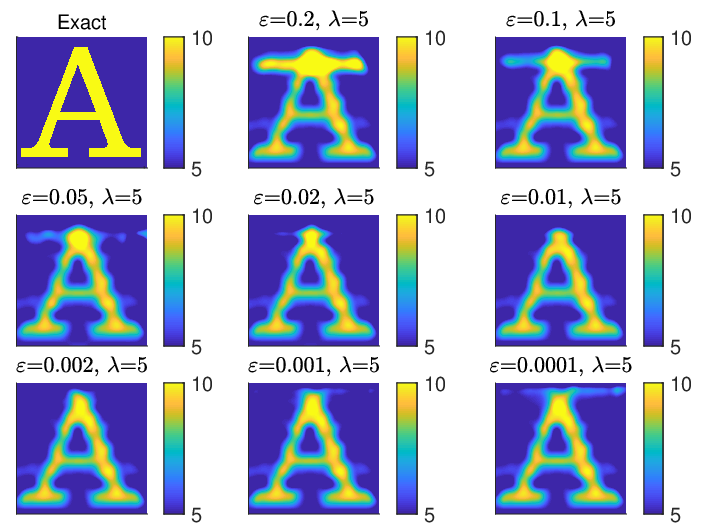
Refer to caption
Figure 2: Test 1. The reconstructed coefficient a⁡(x)a(x), where the function μa​(x)\mu_{a}(x) is given in (6) with ca=5c_{a}=5 inside of the letter ‘A’. We choose λ=5,γ=0.001\lambda=5,\gamma=0.001, and test different values of ε\varepsilon. The reconstruction is not good for ε∈[0.05,0.2]\varepsilon\in\left[0.05,0.2\right]. On the other hand, the quality of the reconstruction improves when ε\varepsilon decreases while ranging from 0.2 to 0.01. While ε\varepsilon varies from 0.01 to 0.001, the difference between the reconstructions is very small. On the other hand, the choice ε=0.0001\varepsilon=0.0001 leads to a lower quality reconstruction quality of the top of letter ‘AA’. Thus, we choose ε=0.01\varepsilon=0.01 as an optimal value and use this value in all follow up tests.

Now we want to select an optimal value of the parameter λ.\lambda. We take γ=0.001,ε=0.01\gamma=0.001,\varepsilon=0.01 and test values λ=0,2,3,4,5,6,8,20\lambda=0,2,3,4,5,6,8,20. Results are presented on Figure 3. The parameter λ\lambda cannot be neither too small nor too large. The reconstructions are unsatisfactory for λ=0,2,20\lambda=0,2,20. On the other hand, the reconstructions become better when λ\lambda ranges from 3 to 5, and they are stabilized for λ=5,6,8\lambda=5,6,8. Thus, we choose λ=5\lambda=5 as the optimal value, see items 2 and 3 of Remarks 5.1 for a relevant discussion.

In summary, we use in the tests below

γ=0.001,ε=0.01,λ=5.\gamma=0.001,\varepsilon=0.01,\lambda=5. (6.20)
Refer to caption
Figure 3: Test 1. The reconstructed coefficient a⁡(x)a(x), where the function μa​(x)\mu_{a}(x) is given in (6) with ca=5c_{a}=5 inside of the letter ‘A’. We choose γ=0.001,ε=0.01\gamma=0.001,\varepsilon=0.01, and test different values of λ\lambda. The reconstructions are unsatisfactory when λ\lambda is too small, λ=0,2\lambda=0,2. Next, the reconstruction quality is improved when λ\lambda changes between 3 and 5, and it is stabilized for λ=5,6,8\lambda=5,6,8. On the other hand, the reconstruction quality deteriorates at λ=20\lambda=20. Thus, we choose λ=5\lambda=5 as the optimal value.

Test 2. We take the same values of parameters as listed in (6.20). We consider the coefficient a⁡(x)a(x) corresponding to μa​(x)\mu_{a}(x) in (6) with ca=10,15,20,30c_{a}=10,15,20,30 inside of the letter ‘AA’. Hence, the inclusion/background contrasts in (6.7) are respectively 3:13:1, 4:14:1, 5:15:1 and 7:17:1. Noise (6.19) in the data is not added. The results are displayed in Figure 4. The reconstruction quality is good for these four cases, although it slightly deteriorates at c=20c=20 and c=30c=30. The computed inclusion/background contrasts (6.8) are accurate.

Refer to caption
Figure 4: Test 2. Exact (top) and reconstructed (bottom) coefficient a⁡(x)a(x) with ca=10,15,20,30c_{a}=10,15,20,30 inside of the letter ‘A’ as in (6) for the values of the parameters being the same as in (6.20). The inclusion/background contrasts in (6.8) are respectively 3:13:1 , 4:14:1, 5:15:1 and 7:17:1. Even though there is a small deterioration at ca=20c_{a}=20 and ca=30c_{a}=30, the accuracy of the reconstruction remains basically the same for these four choices of cac_{a}. The computed inclusion/background contrasts in (6.8) are accurate..

Test 3. We use the same values of parameters as ones in (6.20). We consider the coefficient a⁡(x)a(x) corresponding to μa​(x)\mu_{a}(x) in (6) with ca=5c_{a}=5 inside of the letter ‘Ω\Omega’. Noise (6.19) in the data is not added. The result is displayed in Figure 5. The reconstruction is quite accurate.
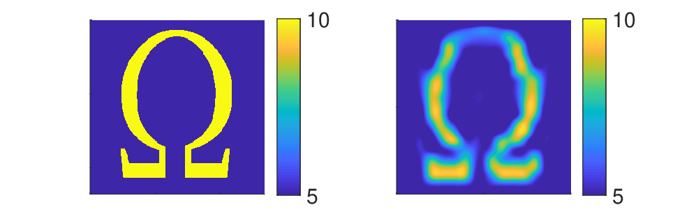
Refer to caption
Figure 5: Test 3. Exact (left) and reconstructed (right) coefficient a⁡(x)a(x) with the shape of the letter ‘Ω\Omega’ with ca=5c_{a}=5 in (6). The values of the parameters are the same as ones in (6.20). The reconstruction is accurate, also, see (6.7) and (6.8).

Test 4. We consider the coefficient a⁡(x)a(x) corresponding to μa​(x)\mu_{a}(x) in (6) with ca=5c_{a}=5 inside of two letters ‘SZ’, which are two letters in the name of the city (Shenzhen) were the second and the third authors reside. Noise (6.19) in the data is not added. Results are exhibited in Figure 6. The reconstruction is worse than the one for the case of the single letter ‘Ω\Omega’ in Figure 5. Nevertheless, the reconstruction is still good and the computed inclusion/background contrasts in (6.8) are both accurate in these two letters.
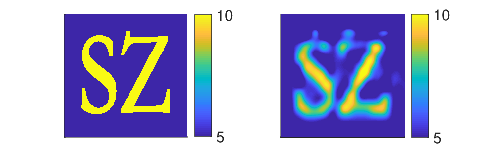
Refer to caption
Figure 6: Test 4. Exact (left) and reconstructed (right) coefficient a⁡(x)a(x) for μa​(x)\mu_{a}(x) in (6) with ca=5c_{a}=5 inside of two letters ‘SZ’. The values of the parameters are the same as ones in (6.20).The reconstruction is worse than the one for the case of the single letter ‘Ω\Omega’ in Figure 5. Nevertheless, the reconstruction is still good and the computed inclusion/background contrasts in (6.8) are accurate in both letters.

Test 5. We now consider the noisy data, as in (6.19), with δ=0.03\delta=0.03 and δ=0.05,\delta=0.05, i.e. with 3% and 5% noise level. We reconstruct the coefficient a⁡(x)a(x) with the shape of the letters ‘A’ and ‘Ω\Omega’ corresponding to μa​(x)\mu_{a}(x) in (6) with ca=5c_{a}=5 inside of two letters. The results are displayed in Figure 7. In all these four cases, reconstructions of shapes of inclusions and the inclusion/background contrasts in (6.8) are accurate.
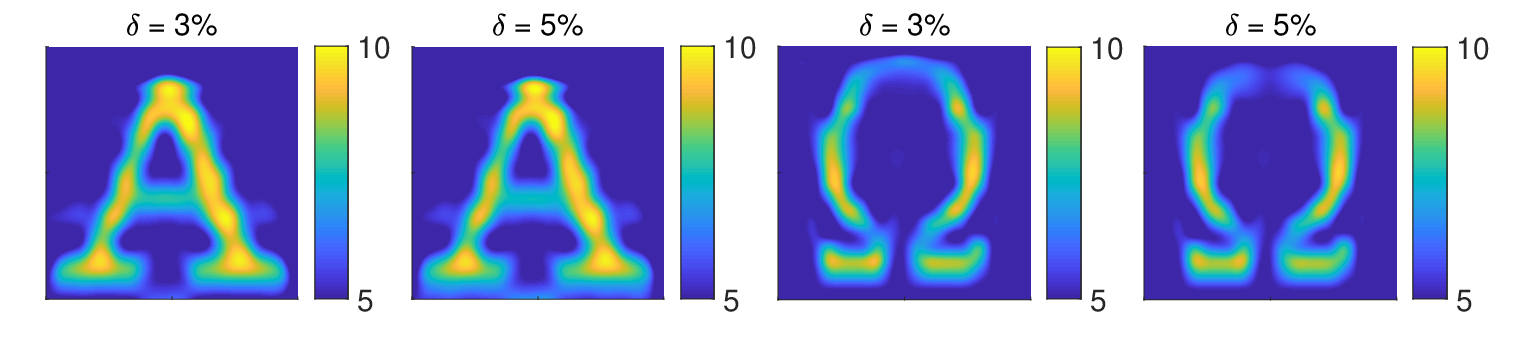
Refer to caption
Figure 7: Test 5. Reconstructed coefficient a⁡(x)a(x) with the shape of letters ‘A’ and ‘Ω\Omega’ with ca=5c_{a}=5 from noisy data (6.19) with δ=0.03\delta=0.03 and δ=0.05\delta=0.05, i.e. with 3% and 5% noise level. The values of the parameters are the same as ones in (6.20). In all these four cases, both reconstructions and the inclusion/background contrasts in (6.8) are accurate.

References

References

  • [1] M. Asadzadeh and L. Beilina. Stability and convergence analysis of a domain decomposition FE/FD method for Maxwell’s equations in the time domain. Algorithms, 15:337, 2022.
  • [2] M. Asadzadeh and L. Beilina. A stabilized p1 domain decomposition finite element method for time harmonic Maxwell’s equations. Math. Comput. Simul, 204:556–574, 2023.
  • [3] A. B. Bakushinskii, M. V. Klibanov, and N. A. Koshev. Carleman weight functions for a globally convergent numerical method for ill-posed Cauchy problems for some quasilinear PDEs. Nonlinear Anal. Real World Appl., 34:201–224, 2017.
  • [4] G. Bal and A. Jollivet. Generalized stability estimates in inverse transport theory. Inverse Probl. Imaging, 12:59–90, 2018.
  • [5] L. Beilina and E. Lindstrom. An adaptive finite element/finite difference domain decomposition method for applications in microwave imaging. Electronics, 11:1359, 2022.
  • [6] L. Beilina and V. Ruas. On the Maxwell-wave equation coupling problem and its explicit finite-element solution. Appl. Math., 68:75–98, 2022.
  • [7] A. L. Bukhgeim and M. V. Klibanov. Uniqueness in the large of a class of multidimensional inverse problems. Soviet Math. Doklady, 17:244–247, 1981.
  • [8] S. Chandrasekhar. Radiative Transfer. Oxford University Press, London, 1950.
  • [9] H. Fujiwara, K. Sadiq, and A. Tamasan. A Fourier approach to the inverse source problem in an absorbing and anisotropic scattering medium. Inverse Probl., 36:015005, 2020.
  • [10] H. Fujiwara, K. Sadiq, and A. Tamasan. Numerical reconstruction of radiative sources in an absorbing and nondiffusing scattering medium in two dimensions. SIAM J. Imaging Sci., 13:535–555, 2020.
  • [11] H. Fujiwara, K. Sadiq, and A. Tamasan. A source reconstrution method in two dimensional radiative transport using boundary data measured on an arc. Inverse Probl., 37:115005, 2021.
  • [12] G. Giorgi, M. Brignone, R. Aramini, and M. Piana. Application of the inhomogeneous Lippmann–Schwinger equation to inverse scattering problems. SIAM J. Appl. Math., 73:212–231, 2013.
  • [13] F. Gölgeleyen and M. Yamamoto. Stability for some inverse problems for transport equations. SIAM J. Math. Anal., 48:2319–2344, 2016.
  • [14] A. V. Goncharsky and S. Y. Romanov. Iterative methods for solving coefficient inverse problems of wave tomography in models with attenuation. Inverse Probl., 33:025003, 2017.
  • [15] A. V. Goncharsky and S. Y. Romanov. A method of solving the coefficient inverse problems of wave tomography. Comput. Math. Appl., 77:967–980, 2019.
  • [16] E. Hassi, S.-E. Chorfi, and L. Maniar. Stable determination of coefficients in semilinear parabolic system with dynamic boundary conditions. Inverse Probl., 38:115007, 2022.
  • [17] J. Heino, S. Arridge, J. Sikora, and E. Somersalo. Anisotropic effects in highly scattering media. Phys. Rev. E, 68:03198, 2003.
  • [18] M. V. Klibanov. Global convexity in a three-dimensional inverse acoustic problem. SIAM J. Math. Anal., 28:1371–1388, 1997.
  • [19] M. V. Klibanov. Carleman estimates for global uniqueness, stability and numerical methods for coefficient inverse problems. J. Inverse Ill-Posed Probl., 21:477–510, 2013.
  • [20] M. V. Klibanov. Convexification of restricted dirichlet to neumann map. J. Inverse Ill-Posed Probl., 25:669–685, 2017.
  • [21] M. V. Klibanov. Stability estimates for some parabolic inverse problems with the final overdetermination via a new Carleman estimate. arXiv, page 2301.09735, 2023.
  • [22] M. V. Klibanov and O. V. Ioussoupova. Uniform strict convexity of a cost functional for three-dimensional inverse scattering problem. SIAM J. Math. Anal., 26:147–179, 1995.
  • [23] M. V. Klibanov, V. A. Khoa, G. W. Bidney, L. H. Nguyen, J. Sullivan, Lam Nguyen, and V. N. Astratov. Convexification inversion method for nonlinear SAR imaging with experimentally collected data. J. Appl. Ind. Math., 15:413–436, 2021.
  • [24] M. V. Klibanov, T. T. Le, and L. H. Nguyen. Convergent numerical method for a linearized travel time tomography problem with incomplete data. SIAM J. Sci. Comput., 42:B1173–B1192, 2020.
  • [25] M. V. Klibanov and J. Li. Inverse Problems and Carleman Estimates: Global Uniqueness, Global Convergence and Experimental Data. De Gruyter, 2021.
  • [26] M. V. Klibanov, J. Li, L. H. Nguyen, V. G. Romanov, and Z. Yang. Convexification numerical method for a coefficient inverse problem for the Riemannian radiative transfer equation. arXiv, page 2212.12593, 2023.
  • [27] M. V. Klibanov, J. Li, L. H. Nguyen, and Z. Yang. Convexification numerical method for a coefficient inverse problem for the radiative transport equation. SIAM J. Imag. Sci., 16:35–63, 2023.
  • [28] M. V. Klibanov, J. Li, and W. Zhang. A globally convergent numerical method for a 3D coefficient inverse problem for a wave-like equations. SIAM J. Sci. Comput., 44:A3341–A3365, 2022.
  • [29] M. V. Klibanov, L. H. Nguyen, and H. V. Tran. Numerical viscosity solutions to Hamilton-Jacobi equations via a Carleman estimate and the convexification method. J. Comput. Phys., 451:110828, 2022.
  • [30] M. V. Klibanov and S. E. Pamyatnykh. Global uniqueness for a coefficient inverse problem for the non-stationary transport equation via Carleman estimate. J. Math. Anal. Appl., 343:352–365, 2008.
  • [31] R. Y. Lai and Q. Li. Parameter reconstruction for general transport equation. SIAM J. Math. Anal., 52:2734–2758, 2020.
  • [32] J. A. Scales, M. L. Smith, and T. L. Fischer. Global optimization methods for multimodal inverse problems. J. Comp. Phys., 103:258–268, 1992.
  • [33] A. V. Smirnov, M. V. Klibanov, and L. H. Nguyen. On an inverse source problem for the full radiative transfer equation with incomplete data. SIAM J. Sci. Comput., 41:B929–B952, 2019.
  • [34] A. N. Tikhonov, A. V. Goncharsky, V. V. Stepanov, and A. G. Yagola. Numerical methods for the solution of ill-posed problems. Kluwer, London, 1995.
  • [35] R. Weissleder and U. Mahmood. Molecular imaging. Radiology, 219:316–333, 2001.