PaGE-Link: Path-based Graph Neural Network Explanation for Heterogeneous Link PredictionConference: Proceedings of the ACM Web Conference 2023; May 1–5, 2023; Austin, TX, USAProceedings of the ACM Web Conference 2023 (WWW ’23), May 1–5, 2023, Austin, TX, USADOI: 10.1145/3543507.3583511ISBN: 978-1-4503-9416-1/23/04CCS: Computing methodologies Neural networksCCS: Mathematics of computing Graph algorithms
Abstract.
Transparency and accountability have become major concerns for black-box machine learning (ML) models. Proper explanations for the model behavior increase model transparency and help researchers develop more accountable models. Graph neural networks (GNN) have recently shown superior performance in many graph ML problems than traditional methods, and explaining them has attracted increased interest. However, GNN explanation for link prediction (LP) is lacking in the literature. LP is an essential GNN task and corresponds to web applications like recommendation and sponsored search on web. Given existing GNN explanation methods only address node/graph-level tasks, we propose Path-based GNN Explanation for heterogeneous Link prediction (PaGE-Link) that generates explanations with connection interpretability, enjoys model scalability, and handles graph heterogeneity. Qualitatively, PaGE-Link can generate explanations as paths connecting a node pair, which naturally captures connections between the two nodes and easily transfer to human-interpretable explanations. Quantitatively, explanations generated by PaGE-Link improve AUC for recommendation on citation and user-item graphs by 9 - 35% and are chosen as better by 78.79% of responses in human evaluation.
Keywords:
Model Transparency, Model Explanation, Graph Neural Networks, Link Prediction1. Introduction
Transparency and accountability are significant concerns when researchers advance black-box machine learning (ML) models (Shin and Park 2019; Lepri et al. 2018). Good explanations of model behavior improve model transparency. For end users, explanations make them trust the predictions and increase their engagement and satisfaction (Herlocker et al. 2000; Bilgic and Mooney 2005). For researchers and developers, explanations enable them to understand the decision-making process and create accountable ML models. Graph Neural Networks (GNNs) (Wu et al. 2020a; Zhou et al. 2020) have recently achieved state-of-the-art performance on many graph ML tasks and attracted increased interest in studying their explainability (Ying et al. 2019; Luo et al. 2020; Zhang et al. 2022; Yuan et al. 2022). However, to our knowledge, GNN explanation for link prediction (LP) is missing in the literature. LP is an essential task of many vital Web applications like recommendation (Zhang et al. 2019; Mao et al. 2021; Wu et al. 2020b) and sponsored search (Li et al. 2021; Hao et al. 2021). GNNs are widely used to solve LP problems (Zhang and Chen 2018; Zhu et al. 2021), and generating good GNN explanations for LP will benefit these applications, e.g., increasing user satisfaction with recommended items.
Existing GNN explanation methods have addressed node/graph-level tasks on homogeneous graphs. Given a data instance, most methods generate an explanation by learning a mask to select an edge-induced subgraph (Ying et al. 2019; Luo et al. 2020) or searching over the space of subgraphs (Yuan et al. 2021). However, explaining GNNs for LP is a new and more challenging task. Existing node/graph-level explanation methods do not generalize well to LP for three challenges. 1) Connection Interpretability: LP involves a pair of the source node and the target node rather than a single node or graph. Desired interpretable explanations for a predicted link should reveal connections between the node pair. Existing methods generate subgraphs with no format constraints, so they are likely to output subgraphs disconnected from the source, the target, or both. Without revealing connections between the source and the target, these subgraph explanations are hard for humans to interpret and investigate. 2) Scalability: For LP, the number of edges involved in GNN computation almost grows from to compared to the node prediction task because neighbors of both the source and the target are involved. Since most existing methods consider all (edge-induced) subgraphs, the increased edges will scale the number of subgraph candidates by a factor of , which makes finding the optimal subgraph explanation much harder. 3) Heterogeneity: Practical LP is often on heterogeneous graphs with rich node and edge types, e.g., a graph for recommendations can have user->buys->item edges and item->has->attribute edges, but existing methods only work for homogeneous graphs.
In light of the importance and challenges of GNN explanation for LP, we formulate it as a post hoc and instance-level explanation problem and generate explanations for it in the form of important paths connecting the source node and the target node. Paths have played substantial roles in graph ML and are the core of many non-GNN LP methods (Liben-Nowell and Kleinberg 2007; Katz 1953; Jeh and Widom 2002; Sun et al. 2011). Paths as explanations can solve the connection interpretability and scalability challenges. Firstly, paths connecting two nodes naturally explain connections between them. Figure 1 shows an example on a graph for recommendations. Given a GNN and a predicted link between user and item , human-interpretable explanations may be based on the user’s preference of attributes (e.g., user bought item that shared the same attribute as item ) or collaborative filtering (e.g, user had a similar preference as user because they both bought item and user bought item , so that user would like item ). Both explanations boil down to paths. Secondly, paths have a considerably smaller search space than general subgraphs. As we will see in Proposition 4.1, compared to the expected number of edge-induced subgraphs, the expected number of paths grows strictly slower and becomes negligible. Therefore, path explanations exclude many less-meaningful subgraph candidates, making the explanation generation much more straightforward and accurate.
To this end, we propose Path-based GNN Explanation for heterogeneous Link prediction (PaGE-Link), which achieves a better explanation AUC and scales linearly in the number of edges (see Figure 2). We first perform k-core pruning (Bollobás 1984) to help find paths and improve scalability. Then we do heterogeneous path-enforcing mask learning to determine important paths, which handles heterogeneity and enforces the explanation edges to form paths connecting source to target. In summary, the contributions of our method are:
- •
Connection Interpretability: PaGE-Link produces more interpretable explanations in path forms and quantitatively improves explanation AUC over baselines.
- •
Scalability: PaGE-Link reduces the explanation search space by magnitudes from subgraph finding to path finding and scales linearly in the number of graph edges.
- •
Heterogeneity: PaGE-Link works on heterogeneous graphs and leverages edge-type information to generate better explanations.
2. Related work
We review relevant research on (a) GNNs (b) GNN explanation (c) recommendation explanation and (d) paths for LP. We summarize the properties of PaGE-Link vs. representative methods in Table 1.
GNNs
GNNs are a family of ML models on graphs (Kipf and Welling 2016; Veličković et al. 2017; Xu et al. 2018). They take graph structure and node/edge features as input and output node representations by transforming and aggregating features of nodes’ (multi-hop) neighbors. The node representations can be used for LP and achieved great results on LP applications (Zhang et al. 2020; Zhang and Chen 2018; Zhang et al. 2019; Mao et al. 2021; Wu et al. 2020b; Zhao et al. 2022; Guo et al. 2022). We review GNN-based LP models in Section 3.
GNN explanation
GNN explanation was studied for node and graph classification, where the explanation is defined as an important subgraph. Existing methods majorly differ in their definition of importance and subgraph selection methods. GNNExplainer (Ying et al. 2019) selects edge-induced subgraphs by learning fully parameterized masks on graph edges and node features, where the mutual information (MI) between the masked graph and the prediction made with the original graph is maximized. PGExplainer (Luo et al. 2020) adopts the same MI importance but trains a mask predictor to generate a discrete mask instead. Other popular importance measures are game theory values. SubgraphX (Yuan et al. 2021) uses the Shapley value (Shapley 1953) and performs Monte Carlo Tree Search (MCTS) on subgraphs. GStarX (Zhang et al. 2022) uses a structure-aware HN value (Hamiache and Navarro 2020) to measure the importance of nodes and generates the important-node-induced subgraph. There are more studies from other perspectives that are less related to this work, i.e., surrogate models (Huang et al. 2020; Vu and Thai 2020), counterfactual explanations (Lucic et al. 2022), and causality (Lin et al. 2021; Lin et al. 2022), for which (Yuan et al. 2020) provides a good review. While these methods produce subgraphs as explanations, what makes a good explanation is a complex topic, especially how to meet “stakeholders’ desiderata” (Langer et al. 2021). Our work differs from all above since we focus on a new task of explaining heterogeneous LP, and we generate paths instead of unrestricted subgraphs as explanations. The interpretability of paths makes our method advantaged especially when stakeholders have less ML background.
Recommendation explanation
This line of works explains why a recommendation is made (Zhang and Chen 2020). J-RECS (Park et al. 2020) generates recommendation explanations on product graphs using a justification score that balances item relevance and diversity. PRINCE (Ghazimatin et al. 2020) produces end-user explanations as a set of minimal actions performed by the user on graphs with users, items, reviews, and categories. The set of actions is selected using counterfactual evidence. Typically, recommendations on graphs can be formalized as an LP task. However, the recommendation explanation problem differs from explaining GNNs for LP because the recommendation data may not be graphs, and the models to be explained are primarily not GNN-based (Wang et al. 2019). GNNs have their unique message passing procedure, and GNN-based LP corresponds to more general applications beyond recommendation, e.g., drug repurposing (Ioannidis et al. 2020), and knowledge graph completion (Nickel et al. 2015; Cheng et al. 2021). Thus, recommendation explanation is related to but not directly comparable to GNN explanation.
Paths
Paths are important in graph ML, and many LP methods are path-based, such as graph distance (Liben-Nowell and Kleinberg 2007), Katz index (Katz 1953), SimRank (Jeh and Widom 2002), and PathSim (Sun et al. 2011). Paths have also been used to capture the relationship between a pair of nodes. For example, the “connection subgraphs” (Faloutsos et al. 2004) find paths between the source and the target based on electricity analogs. In general, although black-box GNNs recently outperform path-based methods in LP accuracy, we embrace paths for their interpretability for LP explanation.
| Methods |
GNNExp (Ying et al. 2019) |
PGExp (Luo et al. 2020) |
SubgraphX (Yuan et al. 2021) |
J-RECS (Park et al. 2020) |
PRINCE (Ghazimatin et al. 2020) |
Rec. Exp. (Zhang and Chen 2020) |
PaGE-Link |
|---|---|---|---|---|---|---|---|
| On Graphs | ✓ | ✓ | ✓ | ✓ | ✓ | ? | ✓ |
| Explains GNN | ✓ | ✓ | ✓ | ✓ | |||
| Explains LP | ? | ? | ? | ✓ | ✓ | ✓ | ✓ |
| Connection | ? | ? | ? | ✓ | |||
| Scalability | ✓ | ✓ | ✓ | ? | ? | ✓ | |
| Heterogeneity | ✓ | ✓ | ✓ | ? | ✓ |
3. Notations and preliminary
In this section, we define necessary notations, summarize them in Table 2, and review the GNN-based LP models.
Definition 3.1.
A heterogeneous graph is defined as a directed graph associated with a node type mapping function and an edge type mapping function . Each node belongs to one node type and each edge belongs to one edge type .
Let denote a trained GNN-based model for predicting the missing links in , where a prediction denotes the predicted link between a source node and a target node . The model learns a conditional distribution of the binary random variable . The commonly used GNN-based LP models (Zhang and Chen 2018; Zhu et al. 2021; Zhao et al. 2022) involve two steps. The first step is to generate node representations of with an -hop GNN encoder. The second step is to apply a prediction head on to get the prediction of . An example prediction head is an inner product.
To explain with an -Layer GNN encoder, we restrict to the computation graph . is the -hop ego-graph of the predicted pair , i.e., the subgraph with node set . It is called a computation graph because the -layer GNN only collects messages from the -hop neighbors of and to compute and . The LP result is thus fully determined by , i.e., . Figure 3(b) shows a 2-hop ego-graph of and , where and are excluded since they are more than 2 hops away from either or .
| Notation | Definition and description |
|---|---|
| a heterogeneous graph , node set , and edge set | |
| a node type mapping function | |
| an edge type mapping function | |
| the degree of node | |
| edges with type , i.e., | |
| the GNN-based LP model to explain | |
| the source and target node for the predicted link | |
| & | the node representations for & |
| the link prediction of the node pair | |
| the computation graph, i.e., L-hop ego-graph of |
4. Proposed problem formulation: link-prediction explanation
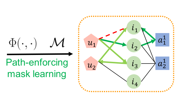
In this work, we address a post hoc and instance-level GNN explanation problem. The post hoc means the model has been trained. To generate explanations, we won’t change its architecture or parameters. The instance level means we generate an explanation for the prediction of each instance . Specifically, the explanation method answers the question of why a missing link is predicted by . In a practical web recommendation system, this question can be “why an item is recommended to a user by the model”.
An explanation for a GNN prediction should be some substructure in , and it should also be concise, i.e., limited by a size budget . This is because an explanation with a large size is often neither informative nor interpretable, for example, an extreme case is that could be a non-informative explanation for itself. Also, a fair comparison between different explanations should consume the same budget. In the following, we define budget as the maximum number of edges included in the explanation.
We list three desirable properties for a GNN explanation method on heterogeneous LP: capturing the connection between the source node and the target node, scalable to large graphs, and addressing graph heterogeneity. Using a path-based method inherently possesses all the properties. Paths capture the connection between a pair of nodes and can be transferred to human-interpretable explanations. Besides, the search space of paths with the fixed source node and the target node is greatly reduced compared to edge-induced subgraphs. Given the ego-graph of and , the number of paths between and and the number of edge-induced subgraphs in both rely on the structure of . However, they can be estimated using random graph approximations. The next proposition on random graphs shows that the expected number of paths grows strictly slower than the expected number of edge-induced subgraphs as the random graph grows. Also, the expected number of paths becomes insignificant for large graphs.
Proposition 4.1.
Let be a random graph with n nodes and density d, i.e., there are edges chosen uniformly randomly from all node pairs. Let be the expected number of paths between any pair of nodes. Let be the expected number of edge-induced subgraphs. Then , i.e., .
Proof.
In Appendix A. ∎
Paths are also a natural choice for LP explanations on heterogeneous graphs. On homogeneous graphs, features are important for prediction and explanation. A - link may be predicted because of the feature similarity of node and node . However, the heterogeneous graphs we focus on, as defined in Definition 3.1, often do not store feature information but explicitly model it using new node and edge types. For example, for the heterogeneous graph in Figure 3(a), instead of making it a user-item graph and assigning each item node a two-dimensional feature with attributes and , the attribute nodes are explicitly created and connected to the item nodes. Then an explanation like “ and share node feature ” on a homogeneous graph is transferred to “ and are connected through the attribute node ” on a heterogeneous graph.
Given the advantages of paths over general subgraphs on connection interpretability, scalability, and their capability to capture feature similarity on heterogeneous graphs, we use paths to explain GNNs for heterogeneous LP. Our design principle is that a good explanation should be concise and informative, so we define the explanation to contain only short paths without high-degree nodes. Long paths are less desirable since they could correspond to unnecessarily complicated connections, making the explanation neither concise nor convincing. For example, in Figure 3(c), the long path is not ideal since it takes four hops to go from item to the item , making it less persuasive to be interpreted as “item1 and item3 are similar so item1 should be recommended”. Paths containing high-degree nodes are also less desirable because high-degree nodes are often generic, and a path going through them is not as informative. In the same figure, all paths containing node are less desirable because has a high degree and connects to all the items in the graph. A real example of a generic attribute is the attribute “grocery” connecting to both “vanilla ice cream” and “vanilla cookie”. When “vanilla ice cream” is recommended to a person who bought “vanilla cookie”, explaining this recommendation with a path going through “grocery” is not very informative since “grocery” connects many items. In contrast, a good informative path explanation should go through the attribute “vanilla”, which only connects to vanilla-flavored items and has a much lower degree.
We formalize the GNN explanation for heterogeneous LP as:
Problem 4.2.
Generating path-based explanations for a predicted link between node and :
- •
Given
- –
a trained GNN-based LP model ,
- –
a heterogeneous computation graph of and ,
- –
a budget of the maximum number of edges in the explanation,
- –
- •
Find an explanation { is a - path with maximum length and degree of each node less than }, ,
- •
By optimizing to be influential to the prediction, concise, and informative.
5. Proposed method: PaGE-Link
This section details PaGE-Link. PaGE-Link has two modules: (i) a -core pruning module to eliminate spurious neighbors and improve speed, and (ii) a heterogeneous path-enforcing mask learning module to identify important paths. An illustration is in Figure 3.
5.1. The k-core Pruning
The -core pruning module of PaGE-Link reduces the complexity of . The -core of a graph is defined as the unique maximal subgraph with a minimum node degree (Bollobás 1984). We use the superscript to denote the -core, i.e., for the -core of . The -core pruning is a recursive algorithm that removes nodes such that their degrees , until the remaining subgraph only has nodes with , which gives the -core. The difference in nodes between a -core and a -core is called the -shell. The nodes in the orange box of Figure 3(b) is an example of a -core pruned from the -hop ego-graph, where node and are pruned in the first iteration because they are degree one. Node is recursively pruned because it becomes degree one after node is pruned. All those three nodes belong to the -shell. We perform -core pruning to help path finding because the pruned -shell nodes are unlikely to be part of meaningful paths when is small. For example, the -shell nodes are either leaf nodes or will become leaf nodes during the recursive pruning, which will never be part of a path unless or are one of these -shell nodes. The -core pruning module in PaGE-Link is modified from the standard -core pruning by adding a condition of never pruning and .
The following theorem shows that for a random graph , -core will reduce the expected number of nodes by a factor of and reduce the expected number of edges by a factor of . Both factors are functions of , , and . We defer the exact expressions of these two factors in Appendix B, since they are only implicitly defined based on Poisson distribution. Numerically, for a random with average node degree , its 5-core has and both .
Theorem 5.1 (Pittel, Spencer and Wormald (Pittel et al. 1996)).
Let be a random graph with edges as in Proposition 4.1. Let be the nonempty -core of . Then contain nodes and edges with high probability for large n, i.e., and ( stands for convergence in probability).
Proof.
Please refer to Appendix B and (Pittel et al. 1996). ∎
The -core pruning helps reduce the graph complexity and accelerates path finding. One concern is whether it prunes too much and disconnects and . We found that such a situation is very unlikely to happen in practice. To be specific, we focus on explaining positively predicted links, e.g. why an item is recommended to a user by the model. Negative predictions, e.g., why an arbitrary item is not recommended to a user by the model, are less useful in practice and thus not in the scope of our explanation. node pairs are usually connected by many paths in a practical (Watts and Strogatz 1998), and positive link predictions are rarely made between disconnected or weakly-connected . Empirically, we observe that there are usually too many paths connecting a positively predicted instead of no paths, even in the -core. Therefore, an optional step to enhance pruning is to remove nodes with super-high degrees. As we discussed in Section 4, high-degree nodes are often generic and less informative. Removing them can be a complement to k-core to further reduce complexity and improve path quality.
5.2. Heterogeneous Path-Enforcing Mask Learning
The second module of PaGE-Link learns heterogeneous masks to find important path-forming edges. We perform mask learning to select edges from the -core-pruned computation graph. For notation simplicity in this section, we use to denote the graph for mask learning to save superscripts and subscripts, and is the actual graph in the complete version of our algorithm.
The idea is to learn a mask over all edges of all edge types to select the important edges. Let be edges with type . Let be learnable masks of all edge types, with corresponds type . We denote applying on its corresponding edge type by , where is the sigmoid function, and is the element-wise product. Similarly, we also overload the notation to indicate applying the set of masks on all types of edges, i.e., . We call the graph with the edge set a masked graph. Applying a mask on graph edges will change the edge weights, which makes GNNs pass more information between nodes connected by highly-weighted edges and less on others. The general idea of mask learning is to learn an that produces high weights for important edges and low weights for others. To learn an that better fits the LP explanation, we measure edge importance from two perspectives: important edges should be both influential for the model prediction and form meaningful paths. Below, we introduce two loss terms and for achieving these two measurements.
is to learn to select influential edges for model prediction. The idea is to do a perturbation-based explanation, where parts of the input are considered important if perturbing them changes the model prediction significantly. In the graph sense, if removing an edge significantly influences the prediction, then is a critical counterfactual edge that should be part of the explanation. This idea can be formalized as maximizing the mutual information between the masked graph and the original graph prediction , which is equivalent to minimizing the prediction loss
| (1) |
has a straightforward meaning, which says the masked subgraph should provide enough information for predicting the missing link as the whole graph. Since the original prediction is a constant, can also be interpreted as the performance drop after the mask is applied to the graph. A well-masked graph should give a minimum performance drop. Regularizations of the mask entropy and mask norm are often included in to encourage the mask to be discrete and sparse.
is the loss term for to learn to select path-forming edges. The idea is to first identify a set of candidate edges denoted by (specified below), where these edges can form concise and informative paths, and then optimize to enforce the mask weights for to increase and mask weights for to decrease. We considered a weighted average of these two forces balanced by hyperparameters and ,
| (2) |
The key question for computing is to find a good containing edges of concise and informative paths. As in Section 4, paths with these two desired properties should be short and without high-degree generic nodes. We thus define a score function of a path reflecting these two properties as below
| (3) | ||||
| (4) |
In this score function, gives the probability of to be included in the explanation, i.e., . To get the importance of a path, we first use a mean-field approximation for the joint probability by multiplying together, and we normalize each for edge by its target node degree . Then, we perform log transformation, which improves numerical stability for multiplying many edges with small or large and break down a path score to a summation of edge scores that are easier to work with. This path score function captures both desired properties mentioned above. A path score will be high if the edges on it have high probabilities and these edges are linked to nodes with low degrees. Finding paths with the highest can be implemented using Dijkstra’s shortest path algorithm (Dijkstra 1959), where the distance represented by each edge is set to be the negative score of the edge, i.e., . We let be the set of edges in the top five shortest paths found by Dijkstra’s algorithm.
5.3. Mask Optimization and Path Generation
We optimize with both and . will increase the weights of the prediction-influential edges. will further increase the weights of the path-forming edges that are also highly weighted by the current and decrease other weights. Finally, after the mask learning converges, we run one more shortest-path algorithm to generate paths from the final and select the top paths according to budget to get the explanation defined in Section 4. A pseudo-code of PaGE-Link is shown in Algorithm 1.
5.4. Complexity Analysis
| GNNExp (Ying et al. 2019) | PGExp (Luo et al. 2020) | SubgraphX (Yuan et al. 2021) | PaGE-Link (ours) |
|---|---|---|---|
| / |
In Table 3, we summarize the time complexity of PaGE-Link and representative existing methods for explaining a prediction with computation graph on a full graph . Let be the mask learning epochs. GNNExplainer has complexity as it learns a mask on . PGExplainer has a training stage and an inference stage (separated by / in the table). The inference stage is linear in , but the training stage covers edges in the entire graph and thus scales in . SubgraphX has a much higher time complexity exponential in , so a size budget of nodes is forced to replace , and denotes the maximum degree (derivation in Appendix C). For PaGE-Link, the k-core pruning step is linear in . The mask learning with Dijkstra’s algorithm has complexity . PaGE-Link has a better complexity than existing methods since is usually smaller than (see Theorem 5.1), and PaGE-Link often converges faster, i.e., has a smaller , as the space of candidate explanations is smaller (see Proposition 4.1) and noisy nodes are pruned.
6. Experiments
In this section, we conduct empirical studies to evaluate explanations generated by PaGE-Link. Evaluation is a general challenge when studying model explainability since standard datasets do not have ground truth explanations. Many works (Ying et al. 2019; Luo et al. 2020) use synthetic benchmarks, but no benchmarks are available for evaluating GNN explanations for heterogeneous LP. Therefore, we generate an augmented graph and a synthetic graph to evaluate explanations. They allow us to generate ground truth explanation patterns and evaluate explainers quantitatively.
6.1. Datasets
The augmented graph
AugCitation is constructed by augmenting the AMiner citation network (Tang et al. 2008). A graph schema is shown in Figure 4(a). The original AMiner graph contains four node types: author, paper, reference (ref), and field of study (fos), and edge types “cites”, “writes”, and “in”. We construct AugCitation by augmenting the original graph with new (author, paper) edges typed “likes” and define a paper recommendation task on AugCitation for predicting the “like” edges. A new edge is augmented if there is at least one concise and informative path between them. In our augmentation process, we require the paths to have lengths shorter than a hyperparameter and with degrees of nodes on (excluding & ) bounded by a hyperparameter . We highlight these two hyperparameters because of the conciseness and informativeness principles discussed in Section 4. The augmented edge is used for prediction. The ground truth explanation is the set of paths satisfying the two hyperparameter requirements. We only take the top paths with the smallest degree sums if there are many qualified paths. We train a GNN-based LP model to predict these new “likes” edges and evaluate explainers by comparing their output explanations with these path patterns as ground truth.
The synthetic graph
UserItemAttr is generated to mimic graphs with users, items, and attributes for recommendations. Figure 4(b) shows the graph schema and illustrates the generation process. We include three node types: “user”, “item”, and item attributes (“attr”) in the synthetic graph, and we build different types of edges step by step. Firstly, the “has” edges are created by randomly connecting items to attrs, and the “hidden prefers” edges are created by randomly connecting users to attrs. These edges represent items having attributes and user preferences for these attributes. Next, we randomly sample a set of items for each user, and we connect a (user, item) pair by a “buys” edge, if the user “hidden prefers” any attr the item “has”. The “hidden prefers” edges correspond to an intermediate step for generating the observable “buys” edges. We remove the “hidden prefers” edges after “buys” edges are generated since we cannot observe ‘hidden prefers” information in reality. An example of the rationale behind this generation step is that items have certain attributes, like the item “ice cream” with the attribute “vanilla”. Then given that a user likes the attribute “vanilla” as hidden information, we observe that the user buys “vanilla ice cream”. The next step is to generate more ‘buys” edges between randomly picked (user, item) pairs if a similar user (two users with many shared item neighbors) buys this item. The idea is like collaborative filtering, which says similar users tend to buy similar items. The final step is generating edges for prediction and their corresponding ground truth explanations, which follows the same augmentation process described above for AugCitation. For UserItemAttr, we have “has” and “buys” as base edges to construct the ground truth, and we create “likes” edges between users and items for prediction.

6.2. Experiment Settings
The GNN-based LP model
As described in Section 3, the LP model involves a GNN encoder and a prediction head. We use RGCN (Schlichtkrull et al. 2018) as the encoder to learn node representations on heterogeneous graphs and the inner product as the prediction head. We train the model using the cross-entropy loss. On each dataset, our prediction task covers one edge type . We randomly split the observed edges of type into train:validation:test = 7:1:2 as positive samples and draw negative samples from the unobserved edges of type . Edges of other types are used for GNN message passing but not prediction.
Explainer baselines.
Existing GNN explanation methods cannot be directly applied to heterogeneous LP. Thus, we extend the popular GNNExplainer (Ying et al. 2019) and PGExplainer (Luo et al. 2020) as our baselines. We re-implement a heterogeneous version of their mask matrix and mask predictor similar to the heterogeneous mask learning module in PaGE-Link. For these baselines, we perform mask learning using their original objectives, and we generate edge-induced subgraph explanations from their learned mask. We refer to these two adapted explainers as GNNExp-Link and PGExp-Link below. We do not compare to other search-based explainers like SubgraphX (Yuan et al. 2021) because of their high computational complexity (see Section 5.4). They work well on small graphs as in the original papers, but they are hard to scale to large and dense graphs we consider for LP.
| GNNExp-Link | PGExp-Link | PaGE-Link (ours) | |
|---|---|---|---|
| AugCitation | 0.829 | 0.586 | 0.928 |
| UserItemAttr | 0.608 | 0.578 | 0.954 |
6.3. Evaluation Results
Quantitative evaluation.
Both the ground truth and the final explanation output of PaGE-Link are sets of paths. In contrast, the baseline explainers generate edge masks . For a fair comparison, we take the intermediate result PaGE-Link learned, also the mask , and we follow (Luo et al. 2020) to compare explainers by their masks. Specifically for each computation graph, edges in the ground truth paths are treated as positive, and other edges are treated as negative. Then weights in are treated as the prediction scores of edges and are evaluated with the ROC-AUC metric. A high ROC-AUC score reflects that edges in ground truth are precisely captured by the mask. The results are shown in Table 4, where PaGE-Link outperforms both baseline explainers.
For scalability, we showed PaGE-Link scales linearly in in Section 5.4. Here we evaluate its scalability empirically by generating ten synthetic graphs with various sizes from 20 to 5,500 edges in . The results are shown in Figure 2b, which suggests the computation time scales linearly in the number of edges.
Qualitative evaluation.
A critical advantage of PaGE-Link is that it generates path explanations, which can capture the connections between node pairs and enjoy better interpretability. In contrast, the top important edges found by baseline methods are often disconnected from the source, the target, or both, which makes their explanations hard for humans to interpret and investigate. We conduct case studies to visualize explanations generated by PaGE-Link on the paper recommendation task on AugCitation.
Figure 5 shows a case in which the model recommends the source author “Vipin Kumar” the recommended target paper titled “Fast and exact network trajectory similarity computation: a case-study on bicycle corridor planning”. The top path explanation generated by PaGE-Link goes through the coauthor “Shashi Shekhar”, which explains the recommendation as Vipin Kumar and Shashi Shekhar coauthored the paper “Correlation analysis of spatial time series datasets: a filter-and-refine approach”, and Shashi Shekhar wrote the recommended paper. Given the same budget of three edges, explanations generated by baselines are less interpretable.
Figure 6 shows another example with the source author “Huan Liu” and the recommended target paper titled “Using association rules to solve the cold-start problem in recommender systems”. PaGE-Link generates paths going through the common fos of the recommended paper and three other papers written by Huan Liu: , , and . We show the PaGE-Link explanation with the top three paths in green. We also show other unselected fos shared by the , , and and the target paper. Note that the explanation paths all have length three, even though there are many paths with length five or longer, e.g., . Also, the explanation paths go through the fos “Redundancy (engineering)” and “User profile” instead of generic fos like “Artificial intelligence” and “Computer science”. This case demonstrates that explanation paths selected by PaGE-Link are more concise and informative.
7. Human Evaluation
The ultimate goal of model explanation is to improve model transparency and help human decision-making. Human evaluation is thus the best way to evaluate the effectiveness of an explainer, which has been a standard evaluation approach in previous works (Selvaraju et al. 2017; Ribeiro et al. 2016; Ghazimatin et al. 2020). We conduct a human evaluation by randomly picking 100 predicted links from the test set of AugCitation and generate explanations for each link using GNNExp-Link, PGExp-Link, and PaGE-Link. We design a survey with single-choice questions. In each question, we show respondents the predicted link and those three explanations with both the graph structure and the node/edge type information, similarly as in Figure 5 but excluding method names. The survey is sent to people across graduate students, postdocs, engineers, research scientists, and professors, including people with and without background knowledge about GNNs. We ask respondents to “please select the best explanation of ‘why the model predicts this author will like the recommended paper?’ ”. At least three answers from different people are collected for each question. In total, 340 evaluations are collected and 78.79% of them selected explanations by PaGE-Link as the best.
8. Conclusion
In this work, we study model transparency and accountability on graphs. We investigate a new task: GNN explanation for heterogeneous LP. We identify three challenges for the task and propose a new path-based method, i.e. PaGE-Link, that produces explanations with interpretable connections, is scalable, and handles graph heterogeneity. PaGE-Link explanations quantitatively improve ROC-AUC by 9 - 35% over baselines and are chosen by 78.79% responses as qualitatively more interpretable in human evaluation.
Acknowledgements.
We thank Ziniu Hu for the helpful discussions on this work. This work is partially supported by NSF (2211557, 1937599, 2119643), NASA, SRC, Okawa Foundation Grant, Amazon Research Awards, Cisco Research Grant, Picsart Gifts, and Snapchat Gifts.References
- (1)
- Bilgic and Mooney (2005) Mustafa Bilgic and Raymond J Mooney. 2005. Explaining recommendations: Satisfaction vs. promotion. In Beyond personalization workshop, IUI, Vol. 5. 153.
- Bollobás (1984) Béla Bollobás. 1984. The evolution of sparse graphs, Graph theory and combinatorics (Cambridge, 1983).
- Cheng et al. (2021) Kewei Cheng, Ziqing Yang, Ming Zhang, and Yizhou Sun. 2021. UniKER: A Unified Framework for Combining Embedding and Definite Horn Rule Reasoning for Knowledge Graph Inference. In Proceedings of the 2021 Conference on Empirical Methods in Natural Language Processing. Association for Computational Linguistics, Online and Punta Cana, Dominican Republic, 9753–9771. https://doi.org/10.18653/v1/2021.emnlp-main.769
- Dijkstra (1959) Edsger W Dijkstra. 1959. A note on two problems in connexion with graphs. Numerische mathematik 1, 1 (1959), 269–271.
- Faloutsos et al. (2004) Christos Faloutsos, Kevin S McCurley, and Andrew Tomkins. 2004. Fast discovery of connection subgraphs. In Proceedings of the tenth ACM SIGKDD international conference on Knowledge discovery and data mining. 118–127.
- Ghazimatin et al. (2020) Azin Ghazimatin, Oana Balalau, Rishiraj Saha Roy, and Gerhard Weikum. 2020. PRINCE: Provider-side interpretability with counterfactual explanations in recommender systems. In Proceedings of the 13th International Conference on Web Search and Data Mining. 196–204.
- Guo et al. (2022) Zhichun Guo, William Shiao, Shichang Zhang, Yozen Liu, Nitesh Chawla, Neil Shah, and Tong Zhao. 2022. Linkless Link Prediction via Relational Distillation. arXiv preprint arXiv:2210.05801 (2022).
- Hamiache and Navarro (2020) Gérard Hamiache and Florian Navarro. 2020. Associated consistency, value and graphs. International Journal of Game Theory 49, 1 (2020), 227–249.
- Hao et al. (2021) Yu Hao, Xin Cao, Yufan Sheng, Yixiang Fang, and Wei Wang. 2021. Ks-gnn: Keywords search over incomplete graphs via graphs neural network. Advances in Neural Information Processing Systems 34 (2021), 1700–1712.
- Herlocker et al. (2000) Jonathan L Herlocker, Joseph A Konstan, and John Riedl. 2000. Explaining collaborative filtering recommendations. In Proceedings of the 2000 ACM conference on Computer supported cooperative work. 241–250.
- (12) Yuval Filmus (https://cs.stackexchange.com/users/683/yuval filmus). 2018. number of connected subgraphs of G with at most k > 0 vertices. (2018). https://cs.stackexchange.com/q/87434
- Huang et al. (2020) Qiang Huang, Makoto Yamada, Yuan Tian, Dinesh Singh, Dawei Yin, and Yi Chang. 2020. GraphLIME: Local Interpretable Model Explanations for Graph Neural Networks. arXiv:2001.06216 [cs.LG]
- Ioannidis et al. (2020) Vassilis N Ioannidis, Da Zheng, and George Karypis. 2020. Few-shot link prediction via graph neural networks for covid-19 drug-repurposing. arXiv preprint arXiv:2007.10261 (2020).
- Janson and Luczak (2008) Svante Janson and Malwina J Luczak. 2008. Asymptotic normality of the k-core in random graphs. The annals of applied probability 18, 3 (2008), 1085–1137.
- Jeh and Widom (2002) Glen Jeh and Jennifer Widom. 2002. Simrank: a measure of structural-context similarity. In Proceedings of the eighth ACM SIGKDD international conference on Knowledge discovery and data mining. 538–543.
- Katz (1953) Leo Katz. 1953. A new status index derived from sociometric analysis. Psychometrika 18, 1 (1953), 39–43.
- Kipf and Welling (2016) Thomas N Kipf and Max Welling. 2016. Semi-supervised classification with graph convolutional networks. arXiv preprint arXiv:1609.02907 (2016).
- Langer et al. (2021) Markus Langer, Daniel Oster, Timo Speith, Holger Hermanns, Lena Kästner, Eva Schmidt, Andreas Sesing, and Kevin Baum. 2021. What do we want from Explainable Artificial Intelligence (XAI)?–A stakeholder perspective on XAI and a conceptual model guiding interdisciplinary XAI research. Artificial Intelligence 296 (2021), 103473.
- Lepri et al. (2018) Bruno Lepri, Nuria Oliver, Emmanuel Letouzé, Alex Pentland, and Patrick Vinck. 2018. Fair, transparent, and accountable algorithmic decision-making processes. Philosophy & Technology 31, 4 (2018), 611–627.
- Li et al. (2021) Chaozhuo Li, Bochen Pang, Yuming Liu, Hao Sun, Zheng Liu, Xing Xie, Tianqi Yang, Yanling Cui, Liangjie Zhang, and Qi Zhang. 2021. Adsgnn: Behavior-graph augmented relevance modeling in sponsored search. In Proceedings of the 44th International ACM SIGIR Conference on Research and Development in Information Retrieval. 223–232.
- Liben-Nowell and Kleinberg (2007) David Liben-Nowell and Jon Kleinberg. 2007. The link-prediction problem for social networks. Journal of the American society for information science and technology 58, 7 (2007), 1019–1031.
- Lin et al. (2021) Wanyu Lin, Hao Lan, and Baochun Li. 2021. Generative causal explanations for graph neural networks. In International Conference on Machine Learning. PMLR, 6666–6679.
- Lin et al. (2022) Wanyu Lin, Hao Lan, Hao Wang, and Baochun Li. 2022. OrphicX: A Causality-Inspired Latent Variable Model for Interpreting Graph Neural Networks. arXiv preprint arXiv:2203.15209 (2022).
- Lucic et al. (2022) Ana Lucic, Maartje A Ter Hoeve, Gabriele Tolomei, Maarten De Rijke, and Fabrizio Silvestri. 2022. Cf-gnnexplainer: Counterfactual explanations for graph neural networks. In International Conference on Artificial Intelligence and Statistics. PMLR, 4499–4511.
- Luo et al. (2020) Dongsheng Luo, Wei Cheng, Dongkuan Xu, Wenchao Yu, Bo Zong, Haifeng Chen, and Xiang Zhang. 2020. Parameterized Explainer for Graph Neural Network. In Advances in Neural Information Processing Systems, H. Larochelle, M. Ranzato, R. Hadsell, M. F. Balcan, and H. Lin (Eds.), Vol. 33. Curran Associates, Inc., 19620–19631.
- Mao et al. (2021) Kelong Mao, Jieming Zhu, Xi Xiao, Biao Lu, Zhaowei Wang, and Xiuqiang He. 2021. UltraGCN: ultra simplification of graph convolutional networks for recommendation. In Proceedings of the 30th ACM International Conference on Information & Knowledge Management. 1253–1262.
- Nickel et al. (2015) Maximilian Nickel, Kevin Murphy, Volker Tresp, and Evgeniy Gabrilovich. 2015. A review of relational machine learning for knowledge graphs. Proc. IEEE 104, 1 (2015), 11–33.
- Park et al. (2020) Namyong Park, Andrey Kan, Christos Faloutsos, and Xin Luna Dong. 2020. J-Recs: Principled and Scalable Recommendation Justification. In 2020 IEEE International Conference on Data Mining (ICDM). IEEE, 1208–1213.
- Pittel et al. (1996) Boris Pittel, Joel Spencer, and Nicholas Wormald. 1996. Sudden emergence of a giantk-core in a random graph. Journal of Combinatorial Theory, Series B 67, 1 (1996), 111–151.
- Ribeiro et al. (2016) Marco Tulio Ribeiro, Sameer Singh, and Carlos Guestrin. 2016. " Why should i trust you?" Explaining the predictions of any classifier. In Proceedings of the 22nd ACM SIGKDD international conference on knowledge discovery and data mining. 1135–1144.
- Roberts and Kroese (2007) Ben Roberts and Dirk P Kroese. 2007. Estimating the Number of st Paths in a Graph. J. Graph Algorithms Appl. 11, 1 (2007), 195–214.
- Schlichtkrull et al. (2018) Michael Schlichtkrull, Thomas N Kipf, Peter Bloem, Rianne van den Berg, Ivan Titov, and Max Welling. 2018. Modeling relational data with graph convolutional networks. In European semantic web conference. Springer, 593–607.
- Selvaraju et al. (2017) Ramprasaath R Selvaraju, Michael Cogswell, Abhishek Das, Ramakrishna Vedantam, Devi Parikh, and Dhruv Batra. 2017. Grad-cam: Visual explanations from deep networks via gradient-based localization. In Proceedings of the IEEE international conference on computer vision. 618–626.
- Shapley (1953) Lloyd Shapley. 1953. A value fo n-person Games. Ann. Math. Study28, Contributions to the Theory of Games, ed. by HW Kuhn, and AW Tucker (1953), 307–317.
- Shin and Park (2019) Donghee Shin and Yong Jin Park. 2019. Role of fairness, accountability, and transparency in algorithmic affordance. Computers in Human Behavior 98 (2019), 277–284. https://doi.org/10.1016/j.chb.2019.04.019
- Sun et al. (2011) Yizhou Sun, Jiawei Han, Xifeng Yan, Philip S Yu, and Tianyi Wu. 2011. Pathsim: Meta path-based top-k similarity search in heterogeneous information networks. Proceedings of the VLDB Endowment 4, 11 (2011), 992–1003.
- Tang et al. (2008) Jie Tang, Jing Zhang, Limin Yao, Juanzi Li, Li Zhang, and Zhong Su. 2008. Arnetminer: extraction and mining of academic social networks. In Proceedings of the 14th ACM SIGKDD international conference on Knowledge discovery and data mining. 990–998.
- Veličković et al. (2017) Petar Veličković, Guillem Cucurull, Arantxa Casanova, Adriana Romero, Pietro Lio, and Yoshua Bengio. 2017. Graph attention networks. arXiv preprint arXiv:1710.10903 (2017).
- Vu and Thai (2020) Minh Vu and My T. Thai. 2020. PGM-Explainer: Probabilistic Graphical Model Explanations for Graph Neural Networks. In Advances in Neural Information Processing Systems, H. Larochelle, M. Ranzato, R. Hadsell, M. F. Balcan, and H. Lin (Eds.), Vol. 33. Curran Associates, Inc., 12225–12235.
- Wang et al. (2019) Xiang Wang, Dingxian Wang, Canran Xu, Xiangnan He, Yixin Cao, and Tat-Seng Chua. 2019. Explainable reasoning over knowledge graphs for recommendation. In Proceedings of the AAAI conference on artificial intelligence, Vol. 33. 5329–5336.
- Watts and Strogatz (1998) Duncan J Watts and Steven H Strogatz. 1998. Collective dynamics of ‘small-world’networks. nature 393, 6684 (1998), 440–442.
- Wu et al. (2020b) Shiwen Wu, Fei Sun, Wentao Zhang, Xu Xie, and Bin Cui. 2020b. Graph neural networks in recommender systems: a survey. ACM Computing Surveys (CSUR) (2020).
- Wu et al. (2020a) Zonghan Wu, Shirui Pan, Fengwen Chen, Guodong Long, Chengqi Zhang, and S Yu Philip. 2020a. A comprehensive survey on graph neural networks. IEEE transactions on neural networks and learning systems 32, 1 (2020), 4–24.
- Xu et al. (2018) Keyulu Xu, Weihua Hu, Jure Leskovec, and Stefanie Jegelka. 2018. How powerful are graph neural networks? arXiv preprint arXiv:1810.00826 (2018).
- Ying et al. (2019) Rex Ying, Dylan Bourgeois, Jiaxuan You, Marinka Zitnik, and Jure Leskovec. 2019. Gnnexplainer: Generating explanations for graph neural networks. Advances in neural information processing systems 32 (2019), 9240.
- Yuan et al. (2020) Hao Yuan, Haiyang Yu, Shurui Gui, and Shuiwang Ji. 2020. Explainability in graph neural networks: A taxonomic survey. arXiv preprint arXiv:2012.15445 (2020).
- Yuan et al. (2022) Hao Yuan, Haiyang Yu, Shurui Gui, and Shuiwang Ji. 2022. Explainability in graph neural networks: A taxonomic survey. IEEE Transactions on Pattern Analysis and Machine Intelligence (2022).
- Yuan et al. (2021) Hao Yuan, Haiyang Yu, Jie Wang, Kang Li, and Shuiwang Ji. 2021. On Explainability of Graph Neural Networks via Subgraph Explorations. In Proceedings of the 38th International Conference on Machine Learning (Proceedings of Machine Learning Research, Vol. 139), Marina Meila and Tong Zhang (Eds.). PMLR, 12241–12252.
- Zhang et al. (2019) Jiani Zhang, Xingjian Shi, Shenglin Zhao, and Irwin King. 2019. Star-gcn: Stacked and reconstructed graph convolutional networks for recommender systems. arXiv preprint arXiv:1905.13129 (2019).
- Zhang and Chen (2018) Muhan Zhang and Yixin Chen. 2018. Link prediction based on graph neural networks. Advances in neural information processing systems 31 (2018).
- Zhang et al. (2020) Muhan Zhang, Pan Li, Yinglong Xia, Kai Wang, and Long Jin. 2020. Revisiting graph neural networks for link prediction. (2020).
- Zhang et al. (2022) Shichang Zhang, Yozen Liu, Neil Shah, and Yizhou Sun. 2022. GStarX: Explaining Graph Neural Networks with Structure-Aware Cooperative Games. In Advances in Neural Information Processing Systems.
- Zhang and Chen (2020) Yongfeng Zhang and Xu Chen. 2020. Explainable Recommendation: A Survey and New Perspectives. Foundations and Trends® in Information Retrieval 14, 1 (2020), 1–101. https://doi.org/10.1561/1500000066
- Zhao et al. (2022) Tong Zhao, Gang Liu, Daheng Wang, Wenhao Yu, and Meng Jiang. 2022. Learning from Counterfactual Links for Link Prediction. In International Conference on Machine Learning. PMLR, 26911–26926.
- Zhou et al. (2020) Jie Zhou, Ganqu Cui, Shengding Hu, Zhengyan Zhang, Cheng Yang, Zhiyuan Liu, Lifeng Wang, Changcheng Li, and Maosong Sun. 2020. Graph neural networks: A review of methods and applications. AI Open 1 (2020), 57–81.
- Zhu et al. (2021) Zhaocheng Zhu, Zuobai Zhang, Louis-Pascal Xhonneux, and Jian Tang. 2021. Neural bellman-ford networks: A general graph neural network framework for link prediction. Advances in Neural Information Processing Systems 34 (2021), 29476–29490.
Appendix A Proof of proposition 4.1
Proof.
We prove by definition, where we show . As we can permute the indices of nodes in , without loss of generality, we assume is the expected number of paths between nodes indexed 1 and n. Our proof is mainly based on the result in (Roberts and Kroese 2007), which computes the expected number of all 1-n paths, i.e., . On the other hand, the number of edge-induced subgraphs considered in (Ying et al. 2019; Luo et al. 2020) equals the size of the power set of all edges, i.e., . We thus have
| (1) | ||||
| (2) | ||||
| (3) | ||||
| (4) | ||||
| (5) | ||||
| (6) | ||||
| (7) | ||||
| (8) | ||||
| (9) | ||||
| (10) | ||||
| (11) | ||||
| (12) |
Step (1) to (2) is Stirling’s formula. Step (8) to (9) is because is continuous. ∎
Appendix B Detailed theorem 5.1
We now state a more detailed version of Theorem 5.1. This theorem gives the exact formula of and , which are built upon a Poisson random variable. The argument is adapted from (Janson and Luczak 2008; Pittel et al. 1996). Readers can refer to (Janson and Luczak 2008; Pittel et al. 1996) for the proof.
For , let denote a Poisson distribution with mean . Let be the tail probability of . Let . When , the equation will have two roots for . Let be the larger root. Then we have the following more detailed version of Theorem 5.1 with and as functions of .
Theorem B.1 (Pittel, Spencer and Wormald).
Let be a random graph with edges as in Proposition 4.1. Let be the k-core of . When , will be nonempty with high probability (w.h.p.) for large n. Also, will contain nodes and edges w.h.p. for large n, i.e., and ( stands for convergence in probability).
Appendix C Complexity of SubgraphX
The search-based methods often have much higher time complexity exponential in the number of nodes or edges. Thus, a budget is forced instead of searching subgraphs with all sizes. For example, SubgraphX finds all connected subgraphs with at most nodes, which has complexity for a graph with maximum degree . This complexity can be shown using the following two lemmas.
Lemma C.1.
For a graph with n vertices, the number of the connected subgraph of having nodes is bounded below by the number of trees in having nodes.
Proof.
Each connected subgraph has a spanning tree. ∎
Lemma C.2.
For a graph with node set , the number of trees in having tree nodes is .
Proof.
See ((2018) https://cs.stackexchange.com/users/683/yuval filmus) for proof using an encoding procedure. ∎
Appendix D Dataset Details
We show the hyperparameters for constructing the datasets in Section 6 in Table 5, which includes the augmentation of the Aminer citation graph and the generation of the synthetic graph.
| AugCitation | 3 | 30 | 5 |
|---|---|---|---|
| UserItemAttr | 3 | 15 | 5 |
Appendix E Path Hit Evaluation
Besides ROC-AUC scores, another way to evaluate the explanations is through the path hit rate (HR). Specifically, we fix the budget of edges and evaluate whether an explanation can hit any complete path in the ground truth. Note that the ground truth for each link only has the top shortest paths with the smallest degree sums, so hitting a long path or a less informative path with high-degree generic nodes will not count.
For a fair comparison with baselines, we take the generated explanation mask for each method, select the top weighted edges to compare against the ground truth. We show results with different budget in Table 6. Explanations generated by PaGE-Link have higher path HR than baselines on both datasets. In contrast, GNNExp-Link and PGExp-Link can barely hit any path in the ground truth for less than 50.
Note that the actual explanation output of PaGE-Link is a set of paths . If we evaluate instead of the top cut of the intermediate output mask . Then PaGE-Link can achieve perfect path HR (=1) when the budget gets large.
| B | GNNExp-Link | PGExp-Link | PaGE-Link (ours) | |
|---|---|---|---|---|
| AugCitation | 10 | 0.000 | 0.000 | 0.007 |
| 50 | 0.002 | 0.000 | 0.194 | |
| 100 | 0.019 | 0.000 | 0.425 | |
| 200 | 0.064 | 0.002 | 0.645 | |
| UserItemAttr | 10 | 0.000 | 0.000 | 0.163 |
| 50 | 0.008 | 0.032 | 0.705 | |
| 100 | 0.016 | 0.039 | 0.790 | |
| 200 | 0.046 | 0.101 | 0.907 |