Learning Visual Representations via Language-Guided Sampling

Mohamed El Banani Karan Desai Justin Johnson Affiliation: University of Michigan Email: {mbanani,kdexd,justincj}@umich.edu

Abstract

Although an object may appear in numerous contexts, we often describe it in a limited number of ways. Language allows us to abstract away visual variation to represent and communicate concepts. Building on this intuition, we propose an alternative approach to visual representation learning: using language similarity to sample semantically similar image pairs for contrastive learning. Our approach diverges from image-based contrastive learning by sampling view pairs using language similarity instead of hand-crafted augmentations or learned clusters. Our approach also differs from image-text contrastive learning by relying on pre-trained language models to guide the learning rather than directly minimizing a cross-modal loss. Through a series of experiments, we show that language-guided learning yields better features than image-based and image-text representation learning approaches.

Refer to caption — Figure 1: Language allows us to find conceptually similar image pairs even if they are visually dissimilar. We use those pairs for contrastive learning to learn generalizable visual features.

1 Introduction

Consider the images in Fig. 1, is the center image more similar to its left or right neighbor? Despite the difference in background and pose, it is clear that the right pair captures the same concept: a flying snow owl. Nevertheless, a self-supervised image model will judge the left pair as more similar. Human perception and language abstract away appearance differences to capture conceptual similarity rather than just visual similarity. Ideally, we could learn visual features that capture conceptual similarity and generalize effectively to other visual tasks. In this work, we show how language can be a proxy for conceptual similarity; allowing us to sample better pairs for contrastive learning and train more generalizable visual models.

Image-only contrastive learning uses visual similarity as a proxy for conceptual similarity. This is based on the observation that discriminative approaches can discover inter-class similarity–e.g., cheetahs are similar to lions– without requiring explicit annotations wu2018unsupervised. The core idea is to train a discriminative model where each instance is treated as a separate class, and the model is trained to map augmented views of the same image to similar features chen2020mocov2; chen2020big; chen2020simple; chen2021exploring; wu2018unsupervised. While successful, instance discrimination ignores the similarity between different instances as it assumes all other images are unrelated. Later work focused on inter-image relationships by estimating clusters asano2019sela; caron2018deepcluster; caron2020unsupervised or finding nearest neighbors dwibedi2021nnclr. However, those relationships are estimated using visual embeddings; resulting in visually, rather than conceptually, similar pairs.

Language similarity is a strong proxy for semantic relationships. Consider the example in Fig. 1; images that depict the same concept are often described similarly. Radford et al. radford2021learning propose language-image contrastive learning by mapping images and text to a shared representation space and achieve impressive generalization capabilities. However, it is unclear whether forcing models to map onto a shared space is optimal for visual learning. Although linguistic and visual similarity might align for similar instances, it is unclear whether all distances in one space should map exactly to the other. Instead of learning a joint vision-and-language representations, we argue that it is better to use linguistic similarity to guide visual learning.

To this end, we propose language-guided contrastive learning: a simple adaptation to contrastive learning that uses language models to find conceptually-similar image pairs for visual learning. Our approach is motivated by the observation that language models, despite never training on visual data, can still be used to sample caption pairs that belong to conceptually similar images, as seen in Fig. 2. Such sampled images exhibit desirable variations in pose, lightning, and context which are very different from hand-crafted augmentations which can be ill-suited to downstream tasks xiao2020should or too focused on background textures selvaraju2021cast. We use the sampled pairs instead of image augmentations within standard self-supervised visual learning approaches such as SimCLR chen2020simple, SimSiam chen2021exploring, and SLIP mu2021slip. Our approach departs from image-only contrastive learning by relying on conceptually-similar image pairs rather than visually similar augmentations or cluster-assignment. We also depart from image-text pre-training by allowing the model to be guided by language similarity rather than learning a joint embedding space.

We conduct a series of controlled experiments to analyze our approach and compare it to commonly used representation learning paradigms on generalization to downstream classification tasks. In controlled settings, our approach outperforms all baselines on linear probe and fewshot classification on a range of downstream classification datasets. Our analysis suggests that while learning multi-modal joint embeddings can result in good representations, it is better to use one modality to guide the training of the other. Furthermore, we find that our approach is robust to the specific choice of sampling strategy or language model. Our code and pre-trained models are available at https://github.com/mbanani/lgssl.

2 Related Work

Visual Representation Learning aims to learn visual embedding spaces that capture semantics, with a typical focus on learning from scalable data sources. Broadly speaking, there are two general approaches: generative and discriminative. Generative approaches hypothesize that a model that can capture the image distribution will learn semantically relevant features gidaris2018unsupervised; doersch2015unsupervised; zhang2016colorful; oord2018representation; he2022masked; vincent2008extracting. In contrast, discriminative approaches posit that differentiating between images will give rise to better features. This idea can be traced by to early work on metric learning chopra2005learning and dimensionality reduction hadsell2006dimensionality, and is clearly seen for supervised classification models sharif2014cnn. More recently, Wu et al. wu2018unsupervised proposed treating each image as a separate class and using augmented images as class instances to relieve the need for human annotation. This was followed by papers that simplified this approach chen2020simple; chen2020big; he2019moco; chen2020mocov2 and proposed non-contrastive variants chen2021exploring; grill2020bootstrap. While those approaches have been successful, the utility of augmentation-based self-supervised learning has been questioned newell2020useful; xiao2020should with follow-up work proposing the use of objectness peng2022crafting; mishra2021object and saliency selvaraju2021cast to alleviate some of those concerns. While we share the goal of visual representation learning, we question the reliance on image augmentations for training and propose using language models to learn for conceptually-similar images.

Language-supervised vision pre-training aims to learn visual representations from language data. Early work of Li et al. li2017ngrams trained n-gram models using YFCC yfcc100m images and user-tag metadata. While some works learn joint vision-and-language representations for tasks like visual question answering antol2015vqa; zhu2016visual7w; goyal2017making; hudson2019gqa, visual reasoning suhr2019corpus; zellers2019recognition; kazemzadeh2014referitgame, and retrieval young2014image; park2022normalized, we are interested in using language to learn better visual representations desai2021virtex; desai2021virtex; sariyildiz2020learning; radford2021learning; stroud2020learning. Early works used language modeling as a pretext task for visual learning sariyildiz2020learning; desai2021virtex, but contrastive approaches quickly gained more popularity due to their relative simplicity and generalization capabilities radford2021learning; jia2021scaling. Follow-up work extended the contrastive formulation to learn dense features yao2022filip; xu2022groupvit or used additional self-supervised losses to improve performance and data efficiency li2022declip; cui2022democratizing; mu2021slip; lee2022uniclip. While we share the motivation of using language for visual learning, we focus on learning visual representations by using linguistic guidance from pre-trained language models.

Leveraging structure in the data. This is commonly done in dense feature learning, where optical flow han2020coclr; wang2019learning; jabri2020space; shan2021cohesiv or 3D transformations hou2021pri3d; Wu2021Towers; shang2022learning; elbanani2021unsupervisedr; sun2021loftr provide natural associations between image patches. For images, prior approaches used class names roth2022integrating; khosla2020supervised, class hierarchies li2019large; yan2015hd, meta data johnson2015love; li2017ngrams; gong2014multi or clustering caron2018deepcluster; caron2020unsupervised; asano2019sela; tian2021divide; zheng2021weakly to improve learning and inference. Within contrastive learning, clustering has been a popular choice for leveraging dataset structure. The intuition is that natural clusters emerge in feature spaces that can provide an additional training signal or useful pseudo-labels. While such approaches work well on curated datasets (e.g., ImageNet) where the label set provides an estimate of the number of clusters, it struggles with imbalanced and uncurated data assran2023hiddenprior. Other approaches sample nearest neighbors as a feature-driven within-domain augmentation dwibedi2021nnclr; li2022declip. While these approaches differ in how they extract inter-instance relationships, they all use within-domain feature similarity to sample positive pairs or clusters and hence do not leverage the rich cross-modal relationships. Closest to our work is Han et al. han2020coclr who propose a co-training blum1998combining scheme for jointly learning image and optical flow representations. We share their motivation of using similarity in one space (language) to learn in another (vision). Furthermore, instead of relying on co-training on the same dataset, we extract distances from a text-only language model, allowing us to leverage unaligned data.

3 Method

The goal of this work is to learn visual representations that can generalize to other datasets. We extend image-only contrastive learning beyond hand-crafted augmentations and visually-sampled clusters to learn from conceptually similar images. Through learning to associate images that depict the same visual concept, models can learn visual invariances that more closely capture human semantics. To achieve this, we propose sampling image pairs that have similar captions using a pre-trained sentence encoder reimers2019sbert and using them for contrastive learning. This work does not propose a new model or loss but rather a novel way of sampling image views that is applicable to a variety of approaches and losses for learning visual representations.

3.1 Learning from Conceptual Similarity

Instance discrimination has been the dominant task for visual representation learning. Its core intuition is that visual similarity is a good proxy for semantic similarity. The standard approach generates positive view pairs using image augmentations and maximizes their embedding similarity, with or without negative views. While there has been a large number of contrastive learning approaches, view pair generation has largely remained the same. Other methods use visual feature similarity to learn prototypes asano2019sela; caron2018deepcluster; caron2020unsupervised or sample previously seen instances dwibedi2021nnclr for contrastive learning. While these approaches extend beyond instances and consider relations in the dataset, they still rely on visual similarity to generate their contrastive pairs. This limits the visual invariances that they can learn xiao2020should.

We propose training models to identify the same visual concept instead of the same instance. Our key observation is simple: images that have similar captions often depict similar concepts regardless of the actual appearance similarity. This can be clearly seen in Fig. 2. Nearest neighbors in visual representation space depict objects in similar scenes and poses, with self-supervised models showing some color invariances due to color augmentation. Conversely, similarly captioned images depict objects in different colors, poses, and contexts. This makes language-sampled images an excellent source for visual representation learning as they implicitly capture human-like visual invariances.

3.2 Sampling Image Pairs using Language

Given a captioned image dataset, we want to sample image pairs that have very similar captions. While caption similarity may be a good proxy for conceptual similarity, measuring caption similarity is a challenge on its own. Traditional metrics such as BLEU papineni2002bleu and CIDER vedantam2015cider rely on n-gram overlap, which can be too sensitive to phrasing and sentence structure. This makes them ill-suited for our needs. Other metrics such as SPICE anderson2016spice account for such variety by comparing parse trees; however, they still can not account for different wording choices. Inspired by advances in language models as well as approaches like BERTScore zhang2019bertscore and CLIPScore hessel2021clipscore, we use a pre-trained sentence encoder to compute caption similarity.

Sentence encoders are trained to extract sentence-level features reimers2019sbert; logeswaran2018efficient; kiros2015skip. We use SBERT reimers2019sbert, which fine-tunes a pre-trained language model to allow it to better capture semantic similarity using feature cosine distance. SBERT is trained in two stages: first, a language backbone is trained using a standard self-supervised task such as masked mikolov2013distributed; devlin2018bert or permuted song2020mpnet language modeling; second, the language modeled is fine-tuned via contrastive learning on a large combined dataset of 1 billion sentence pairs. Fine-tuning the model in a contrastive way simplifies downstream usage as it allows features to be compared directly using cosine similarity. We use an SBERT reimers2019sbert model with an MPNet song2020mpnet backbone. However, we find that our formulation is not sensitive to the choice of language encoder, as shown in Table 5(c).

Finally, we sample the nearest neighbors for all captions in the language embedding space. We leverage modern similarity search libraries johnson2019faiss to perform the nearest neighbor search quickly, despite the large dataset size. For example, nearest neighbor sampling runs in under 3 hours for RedCaps (12 million instances) on 4 GPUs, with 43 minutes spent on feature extraction and 117 minutes on nearest neighbor search. Furthermore, we find that we could further reduce the complexity of the sampling by only searching within subsets of the data as shown in Appendix E.

3.3 Language-Guided Visual Learning

Our approach is applicable to several representation learning methods as it only changes the training view pairs. We focus on contrastive learning since its fairly minimal setting allows us to analyze the impact of language guidance with minimal confounding factors. We train SimCLR with the language-sampled pairs and refer to it as LGSimCLR. We also evaluate the impact of language guidance on SimSiam chen2021exploring and SLIP mu2021slip, and find that they can similarly benefit from language guidance. We only use random cropping for image augmentations since language-sampled pairs are naturally augmented versions of each other and find that additional augmentations are not helpful. For LGSLIP, we match their setup by applying the CLIP loss only between the source’s image and caption, ignoring an additional loss between the nearest neighbor image and its caption.

4 Experiments

Our experiments evaluate the efficacy of learning visual features from conceptually similar images. We hypothesize that a model trained with language guidance will learn useful visual invariances and better generalize to downstream tasks. We are interested in answering these questions: Does language guidance improve generalization over other pre-training approaches? Does language guidance generalize to other datasets and pre-training approaches? How can language be used for visual pre-training?

4.1 Experimental Setup

We formulate our experimental setup to compare the efficacy of different learning signals. We train models with language-guided sampling and compare them with image-only self-supervised models and image-text contrastive models. We are interested in conducting controlled experiments for a fair comparison.

Recent work in self-supervised learning has demonstrated the impressive impact of scaling radford2021learning; chen2020simple; zhai2022scaling. While such work has shown impressive performance, it has complicated the evaluation as different models are trained on different pretext tasks on different datasets using varying amounts of compute and training recipes. Furthermore, replication is difficult, if not impossible, due to the unavailability of training data or prohibitive compute requirements. Fortunately, several papers report results that indicate that performance patterns often hold at smaller scales radford2021learning; caron2020unsupervised; chen2020simple; mu2021slip; cui2022democratizing. Hence, we conduct our experiments at a scale that allows us to perform a comprehensive evaluation and permits replication by others.

We conduct our experiments with a standard backbone he2016deep on publicly available datasets cc3m; cc12m; desai2021redcaps. To account for variation in training recipes, we retrain all methods from scratch using the same training recipe. We scale down experiments to a level that permits fair comparisons and replication. We also provide system-level comparisons in Table 4 and scaling results in Appendix D.

Training details: We use a ResNet-50 backbone and train all models using the AdamW optimizer loshchilov2019decoupled with a learning rate of $10^{-3}$ and a weight decay of $10^{-2}$ . We use a cosine learning scheduler loshchilov2016sgdr with 5000 warm-up steps. Models are trained using a batch size of 512 for 250k steps; this corresponds to 10.5 epochs on RedCaps. We use a constant number of steps to permit meaningful comparisons between models trained on different datasets.

Evaluation setup: We evaluate all approaches using linear probe and fewshot classification on 15 classification datasets inspired by kornblith2019better; radford2021learning. We use the linear probe evaluation proposed by kornblith2019better and learn a single linear layer using logistic regression. We sweep over a range of cost values and choose the value with the best validation performance. We retrain a classifier on both train and validation splits and report test performance. We also evaluate all approaches on fewshot classification to understand their generalization ability. We use a weighted kNN classifier on frozen support features inspired by prior work showing its effectiveness for fewshot classification wang2019simpleshot. Please see Appendices A and B for more details on evaluation datasets and tasks.

Baselines: While there have been many proposed visual representation learning approaches, they can be grouped into several key directions that differ in the pretext task. We focus our comparison on a few representative approaches to explore the impact of the learning signal. We overview the baselines here and provide more details in Appendix C.

Many of our baselines are variants of contrastive learning as shown in Fig. 3. Contrastive approaches operate over paired source and target feature embeddings: $\bm{z}^{s}$ and $\bm{z}^{t}$ . The goal is to maximize the similarity between the paired embeddings and minimize it with respect to all other embeddings. Given a batch size $N$ and embedding dimension $F$ , $\bm{z}^{s},\bm{z}^{t}\in\mathbb{R}^{N\times F}$ . The contrastive loss sohn2016improved is:

\mathcal{L}(z^{s},z^{t})=-\log\frac{\exp(\mathrm{sim}(\bm{z}^{s}_{i},\bm{z}^{t}_{i})/\tau)}{\sum_{k=1}^{N}\exp(\mathrm{sim}(\bm{z}^{s}_{i},\bm{z}^{t}_{k})/\tau)}~,

(1)

where $\tau$ is a scaling parameter and $\mathrm{sim}(\cdot,\cdot)$ is cosine similarity. Contrastive approaches primarily differ in how the embeddings are computed.

Image-Only Contrastive Learning contrasts features extracted from two randomly augmented views of the same image to perform instance discrimination wu2018unsupervised. We use SimCLR chen2020simple as a representative approach due to its simplicity and strong performance.

Image-Text Contrastive Learning learns by contrasting features extracted from images and their captions. Unlike image-only approaches, this approach can learn semantics from the captions. Radford et al. radford2021learning first proposed this approach and has had several follow-ups that augment it with additional self-supervised losses losses mu2021slip; li2022declip; lee2022uniclip. We use CLIP radford2021learning and SLIP mu2021slip due to their simplicity.

Nearest Neighbor Contrastive Learning contrast source embeddings with retrieved embeddings from a memory bank. The target features are used to retrieve the nearest neighbor embedding from a memory bank of previous batches. Dwibedi et al. dwibedi2021nnclr proposed this approach for image-only contrastive learning, while Li et al. li2022declip proposed adapting this loss for language embeddings. We use NNCLR dwibedi2021nnclr as Visual NNCLR and DeCLIP li2022declip with the CLIP and the language NNS losses as Language NNCLR.

Image-Only Non-Contrastive Learning deviates from the typical contrastive setup by learning without negative samples grill2020bootstrap; chen2021exploring. We use SimSiam as a representative approach due to its simplicity and strong performance.

Cluster-based Contrastive Learning learn by contrasting image features with learned prototypes caron2018deepcluster; caron2020unsupervised; asano2019sela. Prototypes are estimated via clustering or learned jointly with the feature encoder. Caron et al. caron2020unsupervised report that different cluster-based approaches perform similarly when provided with the same algorithmic advances. We use an adapted SwAV without the multi-crop augmentation strategy as it is equally applicable to other methods. We also compare against a pre-trained SwAV checkpoint in Table 4.

Table 1: Linear Probe Evaluations. We train ResNet-50 models on RedCaps and report performance of a linear probe using frozen features on 15 downstream tasks. Models are split based on whether or not they require caption images for training. LGSimCLR outperforms all previous approaches with strong performance gains for fine-grained classification datasets.

Model	Food-101	CIFAR-10	CIFAR-100	CUB	SUN397	Cars	Aircraft	DTD	Pets	Caltech-101	Flowers	STL-10	EuroSAT	RESISC45	PCAM	Mean
SwAV	63.6	81.3	57.5	21.6	47.5	22.9	35.4	68.1	61.1	70.5	78.0	87.7	94.3	79.9	84.3	63.6
SimSiam	64.1	79.9	56.1	28.2	48.3	29.5	41.2	66.2	69.1	73.6	83.6	85.7	94.4	82.1	83.3	65.7
Visual NNCLR	65.4	82.8	60.2	26.6	50.0	26.6	40.9	68.0	65.2	75.4	83.5	88.5	95.3	82.2	83.8	66.3
SimCLR	69.0	82.9	61.6	30.6	52.6	33.7	43.7	69.8	70.5	74.1	86.9	88.0	95.4	84.6	84.4	68.5
Language NNCLR	81.2	83.1	61.9	48.6	56.5	45.1	37.2	68.8	78.1	82.0	90.2	93.4	92.5	81.1	80.7	72.0
CLIP	80.9	84.7	62.7	50.4	57.4	45.8	36.7	67.6	79.8	84.0	91.0	93.5	93.9	82.2	82.6	72.9
SLIP	77.7	87.2	67.0	42.4	58.1	48.7	45.2	72.3	79.5	82.7	92.1	92.7	95.6	85.5	83.4	74.0
LGSimCLR (Ours)	83.2	87.8	69.0	59.3	60.3	62.3	53.4	71.2	81.8	89.4	95.9	94.0	95.6	88.0	81.1	78.2

4.2 Results

We train all approaches with a ResNet-50 backbone on RedCaps and report results in Tables 1 and 3. Our model outperforms all baselines with a significant margin for both evaluations. We analyze the results below through a series of questions.

Does language-guided sampling provide better training pairs than image augmentations? LGSimCLR greatly outperforms SimCLR despite using the same learning objective. By using language sampled pairs instead of image augmentations, LGSimCLR learns stronger invariances. We find that the largest gains arise in fine-grained datasets: Cars, CUB, and Food101. The performance gains can be explained by considering the critique of Xiao et al. xiao2020should: the training augmentations dictate the invariances learned by SimCLR as shown in nearest neighbor samples in Fig. 2. Consider the third row of Fig. 2, while language sampling depicts three Aston Martin cars in different spots, visual nearest neighbors are sports cars in different poses and colors, closely resembling the flip and color augmentations used for training. Similarly in the first row of Fig. 2, visual nearest neighbors depict owls from different species in similar poses, while language sampling retrieves three great horned owls from different viewpoints. These trends are further amplified when features are used directly for fewshot classification. Language guidance allows us to capture relationships that go beyond visual similarity by training on image pairs that capture human semantics.

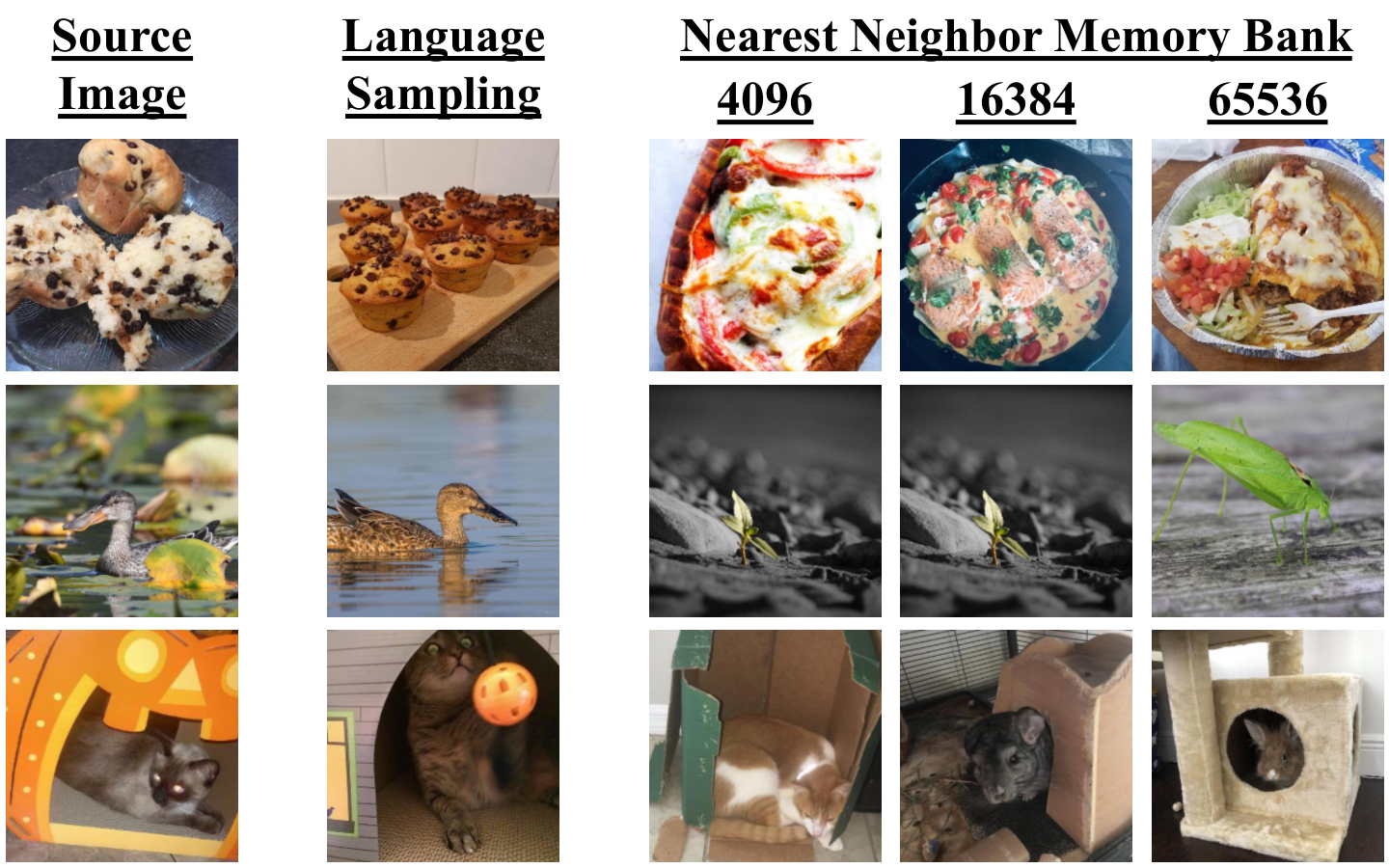
Can we just sample nearest neighbors from previous batches? LGSimCLR outperforms NNCLR despite both relying on nearest neighbors. NNCLR uses the nearest feature embedding from a memory bank in the same modality. The quality of their retrieved samples is limited by the size of the memory bank. To demonstrate this, we visualize the nearest neighbors retrieved by NNCLR for different memory bank sizes in Fig. 4. We find that the retrieval quality is poor even for larger queues. Interestingly, we note that NNCLR also underperforms SimCLR on RedCaps, despite performing better on ImageNet. We posit that ImageNet’s curated distribution explains this: a queue of 16k will most probably contain instances from each class, resulting in both visually and conceptually similar retrievals. Additionally, the quality of nearest neighbors is affected by the sampling feature space; features that are only trained on image augmentations will have limited invariances as shown in Fig. 2. We further explore the impact of sampling space on training in Section 4.3.

Table 2: Language-guided contrastive learning outperforms image-text contrastive learning, regardless of text encoder.

Objective	Text Encoder	Linear	Fewshot
Image-Text	Randomly-Initialized	72.9	77.5
Image-Text	Frozen SBERT	71.8	77.1
Image-Image	Frozen CLIP (RedCaps)	78.3	82.4
Image-Image	Frozen SBERT	78.2	82.5

Table 3: Few-Shot Evaluations. We train ResNet-50 models on RedCaps and report 5-way, 5-shot classification performance. We observe that language results in huge performance gains as shown by the performance of CLIP and LGSimCLR. Furthermore, the use of any augmentations hurts performance as seen by SLIP’s drop in performance.

Model	Food-101	CIFAR-10	CIFAR-100	CUB	SUN397	Cars	Aircraft	DTD	Pets	Caltech-101	Flowers	STL-10	EuroSAT	RESISC45	Mean
SwAV	64.5	54.0	61.8	45.8	84.9	36.5	34.1	74.8	66.5	78.1	75.5	72.6	80.4	72.9	64.5
SimSiam	63.9	49.9	57.2	49.5	84.5	39.3	37.9	75.7	67.8	79.7	81.5	69.6	80.6	79.4	65.5
Visual NNCLR	65.6	54.1	61.7	45.8	85.3	37.9	34.9	75.2	67.3	81.1	75.4	74.3	83.6	76.7	65.6
SimCLR	66.9	45.7	51.0	51.5	87.1	44.0	38.4	77.6	70.1	80.0	86.9	69.6	83.5	81.3	66.7
Language NNCLR	89.3	65.3	73.4	78.6	90.8	68.4	40.4	75.2	78.8	90.9	94.3	89.6	75.2	71.9	77.3
CLIP	88.9	64.6	73.1	78.3	90.9	69.7	40.7	75.7	77.5	91.6	94.7	89.8	75.3	74.8	77.5
SLIP	81.5	63.5	70.8	63.1	91.3	62.9	42.1	79.6	76.4	88.4	92.2	83.4	82.7	80.8	75.6
LGSimCLR (Ours)	90.3	66.3	75.5	83.1	92.7	77.6	50.6	81.1	84.1	95.4	97.6	86.5	85.0	89.0	82.5

Can cluster-based approaches learn better features? Similar to nearest-neighbor sampling, clustering is performed using visual similarity. Furthermore, it is based on an estimated number of clusters in the training dataset. Although this can be determined for ImageNet due to its known class structure, the number of clusters in an arbitrary uncurated dataset is unknown. This results in a large performance drop, as seen in Table 1 and Table 3. On the other hand, sampling related pairs assumes no global structure within the data and hence is able to better capture inter-instance similarity. This results in nearest-neighbor sampling outperforming clustering and both being outperformed by contrastive learning and language-guided contrastive learning.

Should we use language for guidance or supervision? Our experiments indicate that LGSimCLR outperforms both CLIP and SLIP. We consider two possible explanations: (a) SBERT extracts better language embeddings than CLIP can learn from the data, or (b) language-guided contrastive learning is a better training objective than image-text contrastive learning. To evaluate this, we compare four models in Table 2. The first two models use CLIP’s training objective: the first model uses a randomly initialized language encoder, similar to CLIP. The second model uses a frozen SBERT model as the language encoder and only trains the projection layers. The second two models use LGSimCLR’s training objective but sample pairs using a pre-trained language-only SBERT or the language encoder from a CLIP model trained on RedCaps. We find that image-image contrastive learning yields better visual features for both setups. While CLIP does not benefit from an SBERT backbone, LGSimCLR benefits from sampling using a language encoder trained on the same dataset. This suggests that learning joint embeddings results in worse visual features than language-guided learning.

System-level comparisons: We compare LGSimCLR with publicly-available checkpoints of prior approaches; see Appendix C for details. We emphasize that while the experiments reported in Tables 1 and 3 were done in a controlled setup (same batch size, training data, optimizer), the system level comparisons are trained on different datasets with different training recipes and enhancements to further boost performance; e.g., large batch sizes, longer training, multi-crop augmentation. Furthermore, it has been shown that models trained on ImageNet implicitly benefit from its curated nature mu2021slip; assran2023hiddenprior. Nevertheless, our approach still outperforms prior self-supervised approaches. We fall short of CLIP’s ResNet-50 due to its training scale; $64{\times}$ larger batch, $32{\times}$ larger dataset, and 75 ${\times}$ . We also observe that ImageNet-supervised ResNet-50 achieves better fewshot performance. Examining the performance breakdown in Table 10, we find the improvement mainly comes from CIFAR10, CIFAR100, and Pets. We posit that this can be explained by ImageNet’s class structure: mostly pets with a large overlap with CIFAR’s classes.

Table 4: ResNet-50 System Level Comparisons. We outperform prior self-supervised approaches despite them benefiting from ImageNet’s curation for training and using larger batch sizes. CLIP outperforms us due to the scale of its training.

	Batch	# Img Updates	Dataset	Linear	Fewshot
Supervised wightman2021resnet	1024	$1.3{\times}10^{8}$	ImageNet	78.0	85.7
SimSiam chen2021exploring	512	$1.3{\times}10^{8}$	ImageNet	72.9	78.7
SimCLR chen2020big	4096	$1.0{\times}10^{9}$	ImageNet	75.4	77.4
MoCo chen2021mocov3	4096	$1.3{\times}10^{8}$	ImageNet	77.7	80.1
SwAV caron2020unsupervised	4096	$1.3{\times}10^{8}$	ImageNet	78.2	78.5
CLIP radford2021learning	32768	$1.0{\times}10^{10}$	CLIP	81.8	87.8
LGSimCLR	512	$1.3{\times}10^{8}$	RedCaps	78.2	82.5

	Image Aug.		Language
	Linear	Fewshot	Linear	Fewshot
SimSiam	65.7	65.5	71.2	75.7
SimCLR	68.5	66.7	78.2	82.5
SLIP	74.0	75.6	78.8	82.8

(a) Approach Generality

	Size	Linear	Fewshot
CC3M	2.7M	71.5	76.3
CC12M	10.9M	76.8	81.9
RedCaps 2020	3.2M	73.8	78.8
RedCaps	12.0M	78.2	82.5

(b) Impact of training dataset

	Linear	Fewshot
SBERT (MPNet)	78.2	82.5
SBERT (MiniLM)	78.6	83.3
CLIP Language (ViT-B/32)	78.3	83.1
FastText BoW	76.1	80.9
ImageNet-supervised	78.3	81.8
SimCLR (ImageNet)	73.1	74.6

Table 5: Analysis Experiments. We conduct a series of analysis experiments to understand language-guided contrastive learning. The results indicate that language sampling is beneficial to several formulations and scales well with larger datasets. Furthermore, while language sampling consistently results in good pairs for training, visual sampling only helps if it has access to semantics through supervision.

4.3 Analysis

We now analyze language-guided contrastive learning by evaluating the impact of pre-training data, the choice of embedding space, and the pretext task. By understanding the impact of those choices, we can better understand what the model is learning.

Approach generality: We extend language guidance to other contrastive approaches: SimSiam and SLIP. We observe that language guidance uniformly improves performance for all methods, as shown in Table 5(a). Furthermore, the difference between SimCLR and SLIP shrinks when adding language guidance. This suggests that language guidance provides the model with similar semantics to the ones learned from an image-text contrastive loss, resulting in diminished gains from the additional image-text loss.

Impact of training dataset: We train our model on four datasets: CC3M cc3m, CC12M cc12m, RedCaps-2020, and RedCaps desai2021redcaps. In Table 5(b), we observe that larger datasets result in stronger performance, indicating that our approach could scale well with even larger datasets. Furthermore, we observe that RedCaps results in better performance than Conceptual Captions. This may be attributed to the higher quality of captions in RedCaps; while the alt-text captions CC3M and CC12M can be short and contain image metadata, RedCaps captions are diverse, longer, and more descriptive. This allows our model to sample more interesting visual pairs that capture more visual diversity. We provide qualitative results in Appendix F to support this.

Impact of sampling space: The idea of using offline nearest-neighbor sampling does not require a specific language model or even a specific modality. We explore other choices for embedding space: four sentence encoders and two image models. In our experiments, we use SBERT’s MPNet model reimers2019sbert; song2020mpnet; the highest performing SBERT model for sentence similarity. We compare it to two other sentence transformers: a smaller SBERT model, MiniLM wang2020minilm, and the language encoder from CLIP radford2021learning. We also compared against a bag-of-words (BoW) sentence encoder that uses FastText bojanowski2016enriching embeddings. Results are in Table 5(c). While we expected that using CLIP for sampling would improve performance due to its multimodal training, we were surprised that MiniLM also improved performance despite its lower performance on language tasks. We find that pairs obtained using a BoW model result in a weaker performance which might hint at the importance of contextual sentence embeddings. Nevertheless, the BoW-sampled pairs still result in higher performance than all the other baselines on RedCaps.

We also consider training with pairs sampled using two visual models: ImageNet-supervised ResNet-50 wightman2021resnet and ImageNet-trained SimCLR chen2020big. We find that using a visual model for sampling is only beneficial if the visual model captures semantic relations; e.g., through supervised training. Using a self-supervised language model results in a strong drop in performance relative to the other sampling spaces. Nevertheless, it still allows the model to achieve better performance than using a self-supervised visual approach on the same data. This indicates that while language is a better modality to use, “sample-guided” contrastive learning can still achieve a stronger performance than only using self-supervised learning.

Limitations: We observe a few limitations in our approach. Image captions can be noisy, vague, and often omit obvious relations in the image bagherinezhad2016elephants. While this broadly affects image-language models, it can result in us retrieving unrelated image pairs. For example, captions like “I found this in the garden” or “Photo from our family trip” could describe a large range of images, some of which are unrelated. We expand on this in Appendix F. Image descriptions also depend on the context and the perceiver; e.g., a tourist and an art curator will describe artwork in very different ways. We observe that descriptions in topic-focused subreddits (e.g., r/birdpics and r/woodworking) are more specific than in generic subreddits (e.g.,r/itookapicture and r/pics). Our experiments in Appendix E support this observation. Since a caption only captures one aspect of the image, sampled pairs can be similar for a variety of reasons. Allowing the model to condition the feature extraction or similarity calculation on captions could alleviate this issue.

5 Conclusion

We propose using language to find conceptually similar images for contrastive learning. This is based on a simple observation: people describe an object in similar ways even when it appears in different contexts. We use pre-trained language models to sample similar captions and use the captioned images for contrastive learning. We hypothesize that using language guidance instead of image augmentations would result in learning more human-like invariances.

We evaluate our approach on multiple train and test datasets and find that it outperforms previous self-supervised and image-text contrastive models. Our analysis demonstrates the utility of using nearest-neighbor instances for training and the superiority of language sampling over other approaches for unlabeled datasets. Our findings align with prior work that critiques the use of image augmentations xiao2020should; selvaraju2021cast and shows the utility of cross-modal guidance han2020coclr and intra-instance relationships khosla2020supervised; dwibedi2021nnclr. Our results demonstrate the potential of incorporating language guidance in contrastive learning. We hope that future work will explore scaling up our approach to larger and more diverse datasets, as well as modeling approaches that further integrate language into the learning process.

Acknowledgments: We thank Richard Higgins, Ashkan Kazemi, and Santiago Castro for many helpful discussions, as well as David Fouhey, Ziyang Chen, Chenhao Zheng, Fahad Kamran, and Dandan Shan for their feedback on early drafts. This project was funded under the Ford-UM Alliance partnership; we thank Alireza Rahimpour, Devesh Upadhyay, and Ali Hassani from Ford Research for their support and discussion.

References

(1) Peter Anderson, Basura Fernando, Mark Johnson, and Stephen Gould. SPICE: Semantic propositional image caption evaluation. In Proceedings of European Conference on Computer Vision (ECCV), 2016.
(2) Stanislaw Antol, Aishwarya Agrawal, Jiasen Lu, Margaret Mitchell, Dhruv Batra, C Lawrence Zitnick, and Devi Parikh. VQA: Visual question answering. In Proceedings of IEEE International Conference on Computer Vision (ICCV), 2015.
(3) Yuki Markus Asano, Christian Rupprecht, and Andrea Vedaldi. Self-labelling via simultaneous clustering and representation learning. In International Conference on Learning Representations, 2019.
(4) Mido Assran, Randall Balestriero, Quentin Duval, Florian Bordes, Ishan Misra, Piotr Bojanowski, Pascal Vincent, Michael Rabbat, and Nicolas Ballas. The hidden uniform cluster prior in self-supervised learning. In Proceedings of the International Conference on Learning Representations (ICLR), 2023.
(5) Hessam Bagherinezhad, Hannaneh Hajishirzi, Yejin Choi, and Ali Farhadi. Are elephants bigger than butterflies? reasoning about sizes of objects. In AAAI Conference on Artificial Intelligence, 2016.
(6) Avrim Blum and Tom Mitchell. Combining labeled and unlabeled data with co-training. In Proceedings of Annual Conference on Computational learning theory, 1998.
(7) Piotr Bojanowski, Edouard Grave, Armand Joulin, and Tomas Mikolov. Enriching word vectors with subword information. arXiv preprint arXiv:1607.04606, 2016.
(8) Lukas Bossard, Matthieu Guillaumin, and Luc Van Gool. Food-101 – mining discriminative components with random forests. In European Conference on Computer Vision, 2014.
(9) Mathilde Caron, Piotr Bojanowski, Armand Joulin, and Matthijs Douze. Deep clustering for unsupervised learning of visual features. In Proceedings of the European conference on computer vision (ECCV), pages 132–149, 2018.
(10) Mathilde Caron, Ishan Misra, Julien Mairal, Priya Goyal, Piotr Bojanowski, and Armand Joulin. Unsupervised learning of visual features by contrasting cluster assignments. In Advances in Neural Information Processing Systems (NeurIPS), volume 33, 2020.
(11) Soravit Changpinyo, Piyush Sharma, Nan Ding, and Radu Soricut. Conceptual 12M: Pushing Web-Scale Image-Text Pre-Training To Recognize Long-Tail Visual Concepts. In Proceedings of IEEE Conference on Computer Vision and Pattern Recognition (CVPR), 2021.
(12) Ting Chen, Simon Kornblith, Mohammad Norouzi, and Geoffrey Hinton. A Simple Framework for Contrastive Learning of Visual Representations. In Proceedings of the International Conference on Machine Learning (ICML), 2020.
(13) Ting Chen, Simon Kornblith, Kevin Swersky, Mohammad Norouzi, and Geoffrey E Hinton. Big self-supervised models are strong semi-supervised learners. In Advances in Neural Information Processing Systems (NeurIPS), volume 33, 2020.
(14) Xinlei Chen, Haoqi Fan, Ross Girshick, and Kaiming He. Improved baselines with momentum contrastive learning. arXiv preprint arXiv:2003.04297, 2020.
(15) Xinlei Chen and Kaiming He. Exploring simple siamese representation learning. In Proceedings of IEEE Conference on Computer Vision and Pattern Recognition (CVPR), 2021.
(16) Xinlei Chen*, Saining Xie*, and Kaiming He. An empirical study of training self-supervised vision transformers. arXiv preprint arXiv:2104.02057, 2021.
(17) Gong Cheng, Junwei Han, and Xiaoqiang Lu. Remote sensing image scene classification: Benchmark and state of the art. Proceedings of the IEEE, 105(10):1865–1883, Oct 2017.
(18) Sumit Chopra, Raia Hadsell, and Yann LeCun. Learning a similarity metric discriminatively, with application to face verification. In Proceedings of IEEE Conference on Computer Vision and Pattern Recognition (CVPR), 2005.
(19) M. Cimpoi, S. Maji, I. Kokkinos, S. Mohamed, and A. Vedaldi. Describing textures in the wild. In Proceedings of IEEE Conference on Computer Vision and Pattern Recognition (CVPR), 2014.
(20) Adam Coates, Andrew Ng, and Honglak Lee. An Analysis of Single Layer Networks in Unsupervised Feature Learning. In Proceedings of the International Conference on Artificial Intelligence and Statistics (AISTATS), 2011. https://cs.stanford.edu/~acoates/papers/coatesleeng_aistats_2011.pdf.
(21) Yufeng Cui, Lichen Zhao, Feng Liang, Yangguang Li, and Jing Shao. Democratizing contrastive language-image pre-training: A CLIP benchmark of data, model, and supervision. In ICML Workshop on Pre-training: Perspectives, Pitfalls, and Paths Forward, 2022.
(22) Jia Deng, Wei Dong, Richard Socher, Li-Jia Li, Kai Li, and Li Fei-Fei. Imagenet: A large-scale hierarchical image database. In Proceedings of IEEE Conference on Computer Vision and Pattern Recognition (CVPR), 2009.
(23) Karan Desai and Justin Johnson. Virtex: Learning visual representations from textual annotations. In Proceedings of IEEE Conference on Computer Vision and Pattern Recognition (CVPR), pages 11162–11173, 2021.
(24) Karan Desai, Gaurav Kaul, Zubin Aysola, and Justin Johnson. RedCaps: Web-curated image-text data created by the people, for the people. In NeurIPS Datasets and Benchmarks, 2021.
(25) Jacob Devlin, Ming-Wei Chang, Kenton Lee, and Kristina Toutanova. Bert: Pre-training of deep bidirectional transformers for language understanding. Proceedings of the Conference of the North American Chapter of the Association for Computational Linguistics – Human Language Technologies (NAACL HLT), 2018.
(26) Carl Doersch, Abhinav Gupta, and Alexei A Efros. Unsupervised visual representation learning by context prediction. In Proceedings of IEEE International Conference on Computer Vision (ICCV), 2015.
(27) Alexey Dosovitskiy, Lucas Beyer, Alexander Kolesnikov, Dirk Weissenborn, Xiaohua Zhai, Thomas Unterthiner, Mostafa Dehghani, Matthias Minderer, Georg Heigold, Sylvain Gelly, et al. An image is worth 16x16 words: Transformers for image recognition at scale. In Proceedings of the International Conference on Learning Representations (ICLR), 2021.
(28) Debidatta Dwibedi, Yusuf Aytar, Jonathan Tompson, Pierre Sermanet, and Andrew Zisserman. With a little help from my friends: Nearest-neighbor contrastive learning of visual representations. In Proceedings of the IEEE/CVF International Conference on Computer Vision (ICCV), pages 9588–9597, October 2021.
(29) Mohamed El Banani, Luya Gao, and Justin Johnson. Unsupervisedr&r: Unsupervised point cloud registration via differentiable rendering. In Proceedings of the IEEE/CVF Conference on Computer Vision and Pattern Recognition, pages 7129–7139, 2021.
(30) Li Fei-Fei, Rob Fergus, and Pietro Perona. Learning generative visual models from few training examples: An incremental bayesian approach tested on 101 object categories. Computer Vision and Pattern Recognition Workshop, 2004.
(31) Spyros Gidaris, Praveer Singh, and Nikos Komodakis. Unsupervised representation learning by predicting image rotations. In Proceedings of the International Conference on Learning Representations (ICLR), 2018.
(32) Yunchao Gong, Qifa Ke, Michael Isard, and Svetlana Lazebnik. A multi-view embedding space for modeling internet images, tags, and their semantics. In IJCV, 2014.
(33) Yash Goyal, Tejas Khot, Douglas Summers-Stay, Dhruv Batra, and Devi Parikh. Making the V in VQA matter: Elevating the role of image understanding in visual question answering. In Proceedings of IEEE Conference on Computer Vision and Pattern Recognition (CVPR), 2017.
(34) Jean-Bastien Grill, Florian Strub, Florent Altché, Corentin Tallec, Pierre Richemond, Elena Buchatskaya, Carl Doersch, Bernardo Avila Pires, Zhaohan Guo, Mohammad Gheshlaghi Azar, et al. Bootstrap your own latent-a new approach to self-supervised learning. Advances in Neural Information Processing Systems (NeurIPS), 2020.
(35) Raia Hadsell, Sumit Chopra, and Yann LeCun. Dimensionality reduction by learning an invariant mapping. In Proceedings of IEEE Conference on Computer Vision and Pattern Recognition (CVPR), 2006.
(36) Tengda Han, Weidi Xie, and Andrew Zisserman. Self-supervised co-training for video representation learning. In Advances in Neural Information Processing Systems (NeurIPS), 2020.
(37) Kaiming He, Xinlei Chen, Saining Xie, Yanghao Li, Piotr Dollár, and Ross Girshick. Masked autoencoders are scalable vision learners. In Proceedings of IEEE Conference on Computer Vision and Pattern Recognition (CVPR), 2022.
(38) Kaiming He, Haoqi Fan, Yuxin Wu, Saining Xie, and Ross Girshick. Momentum contrast for unsupervised visual representation learning. In Proceedings of IEEE Conference on Computer Vision and Pattern Recognition (CVPR), 2020.
(39) Kaiming He, Xiangyu Zhang, Shaoqing Ren, and Jian Sun. Deep residual learning for image recognition. In Proceedings of IEEE Conference on Computer Vision and Pattern Recognition (CVPR), 2016.
(40) Patrick Helber, Benjamin Bischke, Andreas Dengel, and Damian Borth. Eurosat: A novel dataset and deep learning benchmark for land use and land cover classification. IEEE Journal of Selected Topics in Applied Earth Observations and Remote Sensing, 2019.
(41) Dan Hendrycks, Steven Basart, Norman Mu, Saurav Kadavath, Frank Wang, Evan Dorundo, Rahul Desai, Tyler Zhu, Samyak Parajuli, Mike Guo, Dawn Song, Jacob Steinhardt, and Justin Gilmer. The many faces of robustness: A critical analysis of out-of-distribution generalization. In Proceedings of IEEE International Conference on Computer Vision (ICCV), 2021.
(42) Dan Hendrycks, Kevin Zhao, Steven Basart, Jacob Steinhardt, and Dawn Song. Natural adversarial examples. In Proceedings of IEEE Conference on Computer Vision and Pattern Recognition (CVPR), 2021.
(43) Jack Hessel, Ari Holtzman, Maxwell Forbes, Ronan Le Bras, and Yejin Choi. Clipscore: A reference-free evaluation metric for image captioning. In Proceedings of the Conference on Empirical Methods in Natural Language Processing (EMNLP), 2021.
(44) Ji Hou, Saining Xie, Benjamin Graham, Angela Dai, and Matthias Nießner. Pri3d: Can 3d priors help 2d representation learning? In Proceedings of IEEE International Conference on Computer Vision (ICCV), 2021.
(45) Drew A Hudson and Christopher D Manning. GQA: A new dataset for real-world visual reasoning and compositional question answering. In Proceedings of IEEE Conference on Computer Vision and Pattern Recognition (CVPR), 2019.
(46) Allan Jabri, Andrew Owens, and Alexei Efros. Space-time correspondence as a contrastive random walk. Advances in Neural Information Processing Systems (NeurIPS), 2020.
(47) Chao Jia, Yinfei Yang, Ye Xia, Yi-Ting Chen, Zarana Parekh, Hieu Pham, Quoc Le, Yun-Hsuan Sung, Zhen Li, and Tom Duerig. Scaling up visual and vision-language representation learning with noisy text supervision. In Proceedings of the International Conference on Machine Learning (ICML), 2021.
(48) Justin Johnson, Lamberto Ballan, and Li Fei-Fei. Love thy neighbors: Image annotation by exploiting image metadata. In Proceedings of IEEE International Conference on Computer Vision (ICCV), 2015.
(49) Jeff Johnson, Matthijs Douze, and Hervé Jégou. Billion-scale similarity search with GPUs. IEEE Transactions on Big Data, 2019.
(50) Sahar Kazemzadeh, Vicente Ordonez, Mark Matten, and Tamara Berg. Referitgame: Referring to objects in photographs of natural scenes. In Proceedings of the Conference on Empirical Methods in Natural Language Processing (EMNLP), 2014.
(51) Prannay Khosla, Piotr Teterwak, Chen Wang, Aaron Sarna, Yonglong Tian, Phillip Isola, Aaron Maschinot, Ce Liu, and Dilip Krishnan. Supervised contrastive learning. In Advances in Neural Information Processing Systems (NeurIPS), 2020.
(52) Ryan Kiros, Yukun Zhu, Russ R Salakhutdinov, Richard Zemel, Raquel Urtasun, Antonio Torralba, and Sanja Fidler. Skip-thought vectors. In Advances in Neural Information Processing Systems (NeurIPS), 2015.
(53) Simon Kornblith, Jonathon Shlens, and Quoc V Le. Do better imagenet models transfer better? In Proceedings of the IEEE/CVF conference on computer vision and pattern recognition, pages 2661–2671, 2019.
(54) Jonathan Krause, Michael Stark, Jia Deng, and Li Fei-Fei. 3d object representations for fine-grained categorization. In 4th International IEEE Workshop on 3D Representation and Recognition (3dRR-13), Sydney, Australia, 2013.
(55) Alex Krizhevsky. Learning multiple layers of features from tiny images, 2009.
(56) Janghyeon Lee, Jongsuk Kim, Hyounguk Shon, Bumsoo Kim, Seung Hwan Kim, Honglak Lee, and Junmo Kim. Uniclip: Unified framework for contrastive language-image pre-training. In Advances in Neural Information Processing Systems (NeurIPS), 2022.
(57) Ang Li, Allan Jabri, Armand Joulin, and Laurens van der Maaten. Learning visual n-grams from web data. In Proceedings of IEEE International Conference on Computer Vision (ICCV), 2017.
(58) Aoxue Li, Tiange Luo, Zhiwu Lu, Tao Xiang, and Liwei Wang. Large-scale few-shot learning: Knowledge transfer with class hierarchy. In Proceedings of IEEE Conference on Computer Vision and Pattern Recognition (CVPR), 2019.
(59) Yangguang Li, Feng Liang, Lichen Zhao, Yufeng Cui, Wanli Ouyang, Jing Shao, Fengwei Yu, and Junjie Yan. Supervision Exists Everywhere: A Data Efficient Contrastive Language-Image Pre-training Paradigm. In Proceedings of the International Conference on Learning Representations (ICLR), 2022.
(60) Dong C Liu and Jorge Nocedal. On the limited memory bfgs method for large scale optimization. Mathematical programming, 1989.
(61) Lajanugen Logeswaran and Honglak Lee. An efficient framework for learning sentence representations. In Proceedings of the International Conference on Learning Representations (ICLR), 2018.
(62) Ilya Loshchilov and Frank Hutter. SGDR: Stochastic gradient descent with warm restarts. arXiv preprint arXiv:1608.03983, 2016.
(63) Ilya Loshchilov and Frank Hutter. Decoupled Weight Decay Regularization. In Proceedings of the International Conference on Learning Representations (ICLR), 2019.
(64) Subhransu Maji, Esa Rahtu, Juho Kannala, Matthew Blaschko, and Andrea Vedaldi. Fine-grained visual classification of aircraft. arXiv preprint arXiv:1306.5151, 2013.
(65) Tomas Mikolov, Ilya Sutskever, Kai Chen, Greg S Corrado, and Jeff Dean. Distributed representations of words and phrases and their compositionality. In Advances in Neural Information Processing Systems (NeurIPS), 2013.
(66) Shlok Mishra, Anshul Shah, Ankan Bansal, Abhyuday Jagannatha, Abhishek Sharma, David Jacobs, and Dilip Krishnan. Object-aware cropping for self-supervised learning. arXiv preprint arXiv:2112.00319, 2021.
(67) Norman Mu, Alexander Kirillov, David Wagner, and Saining Xie. Slip: Self-supervision meets language-image pre-training. In Proceedings of European Conference on Computer Vision (ECCV), 2022.
(68) Alejandro Newell and Jia Deng. How useful is self-supervised pretraining for visual tasks? In Proceedings of IEEE Conference on Computer Vision and Pattern Recognition (CVPR), 2020.
(69) M-E. Nilsback and A. Zisserman. Automated flower classification over a large number of classes. In Proceedings of the Indian Conference on Computer Vision, Graphics and Image Processing, Dec 2008.
(70) Aaron van den Oord, Yazhe Li, and Oriol Vinyals. Representation learning with contrastive predictive coding. arXiv preprint arXiv:1807.03748, 2018.
(71) Kishore Papineni, Salim Roukos, Todd Ward, and Wei-Jing Zhu. Bleu: a method for automatic evaluation of machine translation. In Proceedings of the Annual Meeting on Association for Computational Linguistics (ACL), 2002.
(72) Yookoon Park, Mahmoud Azab, Bo Xiong, Seungwhan Moon, Florian Metze, Gourab Kundu, and Kirmani Ahmed. Normalized contrastive learning for text-video retrieval. Proceedings of the Conference on Empirical Methods in Natural Language Processing (EMNLP), 2022.
(73) O. M. Parkhi, A. Vedaldi, A. Zisserman, and C. V. Jawahar. Cats and dogs. In Proceedings of IEEE Conference on Computer Vision and Pattern Recognition (CVPR), 2012.
(74) Adam Paszke, Sam Gross, Francisco Massa, Adam Lerer, James Bradbury, Gregory Chanan, Trevor Killeen, Zeming Lin, Natalia Gimelshein, Luca Antiga, et al. Pytorch: An imperative style, high-performance deep learning library. In Advances in Neural Information Processing Systems (NeurIPS), 2019.
(75) Xiangyu Peng, Kai Wang, Zheng Zhu, Mang Wang, and Yang You. Crafting better contrastive views for siamese representation learning. In Proceedings of IEEE Conference on Computer Vision and Pattern Recognition (CVPR), pages 16031–16040, 2022.
(76) Alec Radford, Jong Wook Kim, Chris Hallacy, Aditya Ramesh, Gabriel Goh, Sandhini Agarwal, Girish Sastry, Amanda Askell, Pamela Mishkin, Jack Clark, et al. Learning transferable visual models from natural language supervision. In Proceedings of the International Conference on Machine Learning (ICML), 2021.
(77) Benjamin Recht, Rebecca Roelofs, Ludwig Schmidt, and Vaishaal Shankar. Do imagenet classifiers generalize to imagenet? In Proceedings of the International Conference on Machine Learning (ICML), 2019.
(78) Nils Reimers and Iryna Gurevych. Sentence-bert: Sentence embeddings using siamese bert-networks. In Proceedings of the 2019 Conference on Empirical Methods in Natural Language Processing. Association for Computational Linguistics, 11 2019.
(79) Karsten Roth, Oriol Vinyals, and Zeynep Akata. Integrating Language Guidance into Vision-based Deep Metric Learning. In Proceedings of IEEE Conference on Computer Vision and Pattern Recognition (CVPR), 2022.
(80) Mert Bulent Sariyildiz, Julien Perez, and Diane Larlus. Learning visual representations with caption annotations. In Proceedings of European Conference on Computer Vision (ECCV), 2020.
(81) Ramprasaath R Selvaraju, Karan Desai, Justin Johnson, and Nikhil Naik. Casting your model: Learning to localize improves self-supervised representations. In Proceedings of IEEE Conference on Computer Vision and Pattern Recognition (CVPR), pages 11058–11067, 2021.
(82) Dandan Shan, Richard Ely Locke Higgins, and David Fouhey. Cohesiv: Contrastive object and hand embedding segmentation in video. In Advances in Neural Information Processing Systems (NeurIPS), 2021.
(83) Jinghuan Shang, Srijan Das, and Michael S Ryoo. Learning viewpoint-agnostic visual representations by recovering tokens in 3d space. Advances in Neural Information Processing Systems (NeurIPS), 2022.
(84) Ali Sharif Razavian, Hossein Azizpour, Josephine Sullivan, and Stefan Carlsson. Cnn features off-the-shelf: an astounding baseline for recognition. In CVPRW, 2014.
(85) Piyush Sharma, Nan Ding, Sebastian Goodman, and Radu Soricut. Conceptual Captions: A cleaned, hypernymed, image alt-text dataset for automatic image captioning. In Proceedings of the Annual Meeting of the Association for Computational Linguistics, 2018.
(86) Kihyuk Sohn. Improved deep metric learning with multi-class n-pair loss objective. In Advances in Neural Information Processing Systems (NeurIPS), 2016.
(87) Kaitao Song, Xu Tan, Tao Qin, Jianfeng Lu, and Tie-Yan Liu. MPNet: Masked and Permuted Pre-training for language understanding. Advances in Neural Information Processing Systems (NeurIPS), 2020.
(88) Jonathan C Stroud, Zhichao Lu, Chen Sun, Jia Deng, Rahul Sukthankar, Cordelia Schmid, and David A Ross. Learning video representations from textual web supervision. arXiv preprint arXiv:2007.14937, 2020.
(89) Alane Suhr, Stephanie Zhou, Ally Zhang, Iris Zhang, Huajun Bai, and Yoav Artzi. A corpus for reasoning about natural language grounded in photographs. In Proceedings of the Annual Meeting on Association for Computational Linguistics (ACL), 2019.
(90) Jiaming Sun, Zehong Shen, Yuang Wang, Hujun Bao, and Xiaowei Zhou. LoFTR: Detector-free local feature matching with transformers. Proceedings of IEEE Conference on Computer Vision and Pattern Recognition (CVPR), 2021.
(91) Igor Susmelj, Matthias Heller, Philipp Wirth, Prescott Jeremey, and Malte Ebner. Lightly. GitHub. Note: https://github.com/lightly-ai/lightly, 2020.
(92) TensorFlow Datasets, a collection of ready-to-use datasets. https://www.tensorflow.org/datasets.
(93) Bart Thomee, David A Shamma, Gerald Friedland, Benjamin Elizalde, Karl Ni, Douglas Poland, Damian Borth, and Li-Jia Li. YFCC100M: The new data in multimedia research. Communications of the ACM, 2016.
(94) Yonglong Tian, Olivier J Henaff, and Aäron van den Oord. Divide and contrast: Self-supervised learning from uncurated data. In Proceedings of the IEEE/CVF International Conference on Computer Vision, 2021.
(95) Yonglong Tian, Yue Wang, Dilip Krishnan, Joshua B Tenenbaum, and Phillip Isola. Rethinking few-shot image classification: a good embedding is all you need? In Proceedings of European Conference on Computer Vision (ECCV), 2020.
(96) Ramakrishna Vedantam, C Lawrence Zitnick, and Devi Parikh. CIDEr: Consensus-based image description evaluation. In Proceedings of IEEE Conference on Computer Vision and Pattern Recognition (CVPR), 2015.
(97) Bastiaan S Veeling, Jasper Linmans, Jim Winkens, Taco Cohen, and Max Welling. Rotation equivariant cnns for digital pathology. In International Conference on Medical image computing and computer-assisted intervention, 2018.
(98) Pascal Vincent, Hugo Larochelle, Yoshua Bengio, and Pierre-Antoine Manzagol. Extracting and composing robust features with denoising autoencoders. In Proceedings of the International Conference on Machine Learning (ICML), 2008.
(99) Haohan Wang, Songwei Ge, Zachary Lipton, and Eric P Xing. Learning robust global representations by penalizing local predictive power. In Advances in Neural Information Processing Systems (NeurIPS), 2019.
(100) Wenhui Wang, Furu Wei, Li Dong, Hangbo Bao, Nan Yang, and Ming Zhou. MiniLM: Deep self-attention distillation for task-agnostic compression of pre-trained transformers. Advances in Neural Information Processing Systems (NeurIPS), 2020.
(101) Xiaolong Wang, Allan Jabri, and Alexei A Efros. Learning correspondence from the cycle-consistency of time. In Proceedings of IEEE Conference on Computer Vision and Pattern Recognition (CVPR), 2019.
(102) Yan Wang, Wei-Lun Chao, Kilian Q. Weinberger, and Laurens van der Maaten. Simpleshot: Revisiting nearest-neighbor classification for few-shot learning. arXiv preprint arXiv:1911.04623, 2019.
(103) P. Welinder, S. Branson, T. Mita, C. Wah, F. Schroff, S. Belongie, and P. Perona. Caltech-UCSD Birds 200. Technical Report CNS-TR-2010-001, California Institute of Technology, 2010.
(104) Ross Wightman, Hugo Touvron, and Herve Jegou. Resnet strikes back: An improved training procedure in timm. In NeurIPS Workshop on ImageNet: Past, Present, and Future, 2021.
(105) Xiaoshi Wu, Hadar Averbuch-Elor, Jin Sun, and Noah Snavely. Towers of babel: Combining images, language, and 3d geometry for learning multimodal vision. In Proceedings of IEEE International Conference on Computer Vision (ICCV), 2021.
(106) Zhirong Wu, Yuanjun Xiong, Stella X Yu, and Dahua Lin. Unsupervised feature learning via non-parametric instance discrimination. In Proceedings of the IEEE conference on computer vision and pattern recognition, pages 3733–3742, 2018.
(107) J. Xiao, J. Hays, K. A. Ehinger, A. Oliva, and A. Torralba. SUN database: Large-scale scene recognition from abbey to zoo. In Proceedings of IEEE Conference on Computer Vision and Pattern Recognition (CVPR), 2010.
(108) Tete Xiao, Xiaolong Wang, Alexei A Efros, and Trevor Darrell. What should not be contrastive in contrastive learning. In International Conference on Learning Representations, 2020.
(109) Jiarui Xu, Shalini De Mello, Sifei Liu, Wonmin Byeon, Thomas Breuel, Jan Kautz, and Xiaolong Wang. Groupvit: Semantic segmentation emerges from text supervision. In Proceedings of IEEE Conference on Computer Vision and Pattern Recognition (CVPR), 2022.
(110) Zhicheng Yan, Hao Zhang, Robinson Piramuthu, Vignesh Jagadeesh, Dennis DeCoste, Wei Di, and Yizhou Yu. Hd-cnn: hierarchical deep convolutional neural networks for large scale visual recognition. In Proceedings of IEEE International Conference on Computer Vision (ICCV), 2015.
(111) Lewei Yao, Runhui Huang, Lu Hou, Guansong Lu, Minzhe Niu, Hang Xu, Xiaodan Liang, Zhenguo Li, Xin Jiang, and Chunjing Xu. FILIP: Fine-grained interactive language-image pre-training. In Proceedings of the International Conference on Learning Representations (ICLR), 2022.
(112) Peter Young, Alice Lai, Micah Hodosh, and Julia Hockenmaier. From image descriptions to visual denotations: New similarity metrics for semantic inference over event descriptions. TACL, 2014.
(113) Rowan Zellers, Yonatan Bisk, Ali Farhadi, and Yejin Choi. From recognition to cognition: Visual commonsense reasoning. In Proceedings of IEEE Conference on Computer Vision and Pattern Recognition (CVPR), 2019.
(114) Xiaohua Zhai, Alexander Kolesnikov, Neil Houlsby, and Lucas Beyer. Scaling vision transformers. In Proceedings of IEEE Conference on Computer Vision and Pattern Recognition (CVPR), 2022.
(115) Richard Zhang, Phillip Isola, and Alexei A Efros. Colorful image colorization. In Proceedings of European Conference on Computer Vision (ECCV), 2016.
(116) Tianyi Zhang, Varsha Kishore, Felix Wu, Kilian Q Weinberger, and Yoav Artzi. Bertscore: Evaluating text generation with bert. In Proceedings of the International Conference on Learning Representations (ICLR), 2019.
(117) Mingkai Zheng, Fei Wang, Shan You, Chen Qian, Changshui Zhang, Xiaogang Wang, and Chang Xu. Weakly supervised contrastive learning. In Proceedings of IEEE International Conference on Computer Vision (ICCV), 2021.
(118) Yuke Zhu, Oliver Groth, Michael Bernstein, and Li Fei-Fei. Visual7w: Grounded question answering in images. In Proceedings of IEEE Conference on Computer Vision and Pattern Recognition (CVPR), 2016.

Appendix A Evaluation Tasks

We compare all models by evaluating the encoder’s frozen features on two downstream classification tasks: linear probe and fewshot. We chose to use simple classifiers since they allow us to evaluate the features as-is and conduct a comprehensive hyperparameter sweep to ensure a fair comparison. We explain the two evaluation setups in more detail below. Our implementation can be found at https://github.com/mbanani/lgssl.

Linear Probe Classification

We follow the linear probe evaluation proposed by Kornblith et al. kornblith2019better of training a logistic regression classifier using the L-BFGS optimizer liu1989limited. We follow prior work kornblith2019better; radford2021learning and perform a hyperparameter sweep over the cost values in the logistic regression loss. We sweep over 96 values in log space from $10^{-6}$ to $10^{6}$ . During the hyperparameter sweep, we train on the train split and validate on the valid split. We choose the cost value with the best validation performance and train a final classifier on the combined train and validation instances. We use the PyTorch paszke2019pytorch implementation of L-BFGS with all the default parameters except for the maximum number of iterations, which is set to 1000 similar to CLIP radford2021learning. Our evaluation metric depends on the dataset, as shown in Table 6, to account for class imbalance.

Few-Shot Classification

We also use fewshot classification as an evaluation for frozen features. Prior work wang2019simpleshot; tian2020rethinking has shown that simple classifiers on top of frozen features are strong baselines for fewshot classification. More specifically, Wang et al. wang2019simpleshot shows that when features are normalized (mean subtraction and L2 normalization), a nearest neighbor classifier is a very effective and strong baseline for fewshot classification. Inspired by these results, we use a simple weighted nearest neighbor classifier to evaluate pre-trained frozen features. We set $k$ to be the size of the support set and classify the features as follows:

\displaystyle y^{\prime}=\argmax_{v}\sum_{(I,y)\in\mathbb{D}_{\text{support}}}\mathbbm{1}_{[v=y]}\mathrm{sim}(f(I^{\prime}),f(I))

(2)

where $\mathbbm{1}_{[v=y]}$ is an indicator variable that is $1$ if $y$ is the same class as $v$ and 0 other wise, $\mathrm{sim}(\cdot,\cdot)$ is cosine similarity between two vectors, $f$ is the visual encoder, $I^{\prime}$ is the target image, $\mathbb{D}_{\text{support}}$ is the support set.

We adopt 5-way, 5-shot classification as our fewshot classification task. We sample five random classes for each episode and then sample five images for each class in the training set, resulting in 25 labeled training images. We also sample 5 images for each class from the test set as our test images. We use all available test images for classes with less than five test images for that class. This is primarily an issue for Caltech-101 feifei2004caltech101. We sample 5000 episodes and compute the average test accuracy across all episodes. We experimented with increasing the number of episodes to 50000 to improve evaluation but noticed little change in the mean performance. We also report the 95% confidence interval for each dataset.

Appendix B Evaluation Datasets

We list all the evaluation datasets used in Table 6. We use TensorFlow datasets for evaluation to ensure easy replication TFDS. For all datasets, we preprocess the images by resizing the image so that its smaller dimension is 224 using bilinear interpolation followed by a center crop to $224{\times}224$ . We use bilinear interpolation since improves performance on low-resolution datasets such as CIFAR-10 and CIFAR-100. We normalize the images using ImageNet’s mean and standard deviation for pixel values for all models except for pre-trained CLIP. For CLIP, we use their provided mean and standard deviation values as they greatly impact performance: an average gain of approximately $4\%$ for linear probe evaluation. We exclude Patch Camelyon from the fewshot evaluation since it is a binary classification dataset. We also include statistics for the ImageNet dataset evaluations done in Appendix G.

Table 6: Evaluation Datasets. Orange rows indicate datasets that do not have an official validation split; we constructed one by randomly holding out 20% of the official train split. Blue rows indicate datasets that do not officially define splits; we randomly sample instances to construct non-overlapping splits. For ImageNet, the validation set is used as the test set, and we construct a validation set by randomly holding out 20% of the official training split. ImageNet variants, highlighted in green, are all test sets for models trained on ImageNet.

Dataset	Classes	Train	Val	Test	Metric
Food-101 bossard2014food101	101	60600	15150	25250	accuracy
CIFAR-10 krizhevsky2009cifar	10	40000	10000	10000	accuracy
CIFAR-100 krizhevsky2009cifar	100	40000	10000	10000	accuracy
CUB-2011 cub200	200	5795	1199	5794	accuracy
SUN397 xiao2010sun397	397	15880	3970	19849	accuracy
Stanford Cars krause2013cars196	196	6515	1629	8041	accuracy
FGVC Aircraft maji2013aircrafts	100	3334	3333	3333	mean-per-cls
DTD cimpoi14describing	47	1880	1880	1880	accuracy
Oxford-IIIT Pets parkhi2012pet	37	2944	736	3669	mean-per-cls
Caltech-101 feifei2004caltech101	102	2448	612	6084	mean-per-cls
Oxford Flowers nilsback2008flowers	102	1020	1020	6149	mean-per-cls
STL-10 coates2011stl10	10	4000	1000	8000	accuracy
EuroSAT helber2019eurosat	10	5000	5000	5000	accuracy
RESISC45 resisc45	45	3150	3150	25200	accuracy
Patch Camelyon veeling2018rotation	2	262144	32768	32768	accuracy
ImageNet deng2009imagenet	1000	1024934	256233	50000	accuracy
ImageNet A hendrycks2019imageneta	200	N/A	N/A	7500	accuracy
ImageNet R hendrycks2020imagenetr	200	N/A	N/A	30000	accuracy
ImageNet v2 recht2019imagenetv2	1000	N/A	N/A	10000	accuracy
ImageNet Sketch wang2019imagenetsketch	1000	N/A	N/A	50889	accuracy

Appendix C Baselines

For fair evaluation, we retrained previous methods from scratch with several methods reimplemented. We also provided several system-level comparisons using pre-trained checkpoints provided by prior work. Below, we provide additional details on our baselines.

Pre-trained model checkpoints

We use publicly available checkpoints of various pre-trained models for sampling and experimental comparisons:

•

SBERT reimers2019sbert: We use two checkpoints from SBERT: all-mpnet-base-v2 (MPNet backbone song2020mpnet), and all-MiniLM-L12-v2 (MiniLM backbone wang2020minilm). Those models were used for sampling, while MPNet was also used as a frozen backbone in analysis experiments.
•

CLIP radford2021learning: We use checkpoints available in the official Github repository¹¹ 1 https://github.com/openai/CLIP for both system-level comparisons and sampling. We use the RN50 checkpoint in the system-level comparisons to match the backbone for other models. We use the ViT-B/32 checkpoint for sampling to provide the strongest visual sampling performance in evaluating different sampling modalities.
•

ImageNet pre-trained model: We use the checkpoints provided by torchvision package.²² 2 https://github.com/pytorch/vision For system-level comparisons, we use the ResNet-50 IMAGENET1K_V2 checkpoint wightman2021resnet as it achieves better performance than the original ResNet-50 checkpoint he2016deep. We also use ViT-B/32 dosovitskiy2021vit checkpoint to compare with the sampling strategy using a CLIP checkpoint.
•

SimCLR chen2020big: We use the SimCLR v2 checkpoint provided by PyTorch Lightning Bolts.³³ 3 https://lightning-bolts.readthedocs.io/ While SimCLR released some checkpoints for TensorFlow, we found that converting them to PyTorch using the recommended tools resulted in lower performance. We use the same checkpoint for both sampling and system-level comparison. Note that SimCLR only released models trained for 800 epochs.
•

SimSiam chen2020simple: We use the checkpoint trained with 512 batch size from the official Github repository⁴⁴ 4 https://github.com/facebookresearch/simsiam as it more closely matches our training setup.
•

MoCo chen2021mocov3: We use the official checkpoint for MoCo v3.⁵⁵ 5 https://github.com/facebookresearch/moco-v3 We use the checkpoint for the model trained for 100 epochs to match other checkpoints more closely.
•

SwAV caron2020unsupervised: We use the official SwAV checkpoint.⁶⁶ 6 https://github.com/facebookresearch/swav We use the checkpoint trained for 100 epochs to match the training duration of other methods. Unlike our implementation, the full SwAV model is trained using Multi-Crop augmentation strategy.

Retrained models

We reimplement and retrain all baselines. When an official implementation was available, we adapted it to fit within our pipeline. For all models, we use a ResNet-50 backbone from torchvision with random initialization and a feature dimension of 2048 (the fc layer is removed). We use a linear layer or a multi-layer perceptron (MLP) for projection layers. Every layer except for the last is followed by batch normalization and a ReLU non-linearity. We describe an N-layer MLP with $N+1$ numbers depicting the input dimension for the first layer, followed by the output dimension for all layers.

We use two forms of augmentation: SimCLR or global crop. Global crop consists of a random resized square crop with a scale of (0.5, 1.0) to an image size of $224{\times}224$ . SimCLR augmentations consist of random resized square crop, color jittering, random grayscale, random horizontal flipping, and Gaussian blur. We use the same augmentation parameters as prior work chen2020big; chen2021mocov3. All images are normalized using ImageNet’s mean and standard deviation statistics.

We provide baseline-specific details below and refer the reader to our implementation for more details:

•

SimCLR: We use a 3-layer MLP as a projection layer with feature dimensions (2048, 2048, 2048, 128) similar to the original paper chen2020big. We use the SimCLR loss implementation from Mu et al. mu2021slip, which adapts the original loss for the distributed settings for inference and gradients. We use SimCLR augmentations for SimCLR and global crop augmentations for LGSimCLR. We experimented with mixing SimCLR augmentation and language sampled pairs and found that it results in slightly inferior performance: adding augmentations reduces the linear probe average accuracy from 78.3 to 77.9.
•

CLIP: We use a linear projection layer to a feature dimension of 512 similar to the original paper. We use the smallest CLIP language encoder, similar to SLIP mu2021slip, with a feature dimension of 512 and a linear language projection layer. We use the loss implementation from SLIP mu2021slip but adapt it to share the loss gradients similar to the SimCLR loss. We use global crop augmentation for CLIP since SLIP mu2021slip reported that it performs better than CLIP’s original center crop preprocessing.
•

SLIP: We follow SLIP’s implementation and combine the augmentations, projections, and losses from SimCLR and CLIP. We use the same language transformer as our CLIP implementation. We generate two augmented views with SimCLR augmentation for the SimCLR loss and one with global cropping for the CLIP loss. Those views are passed through their respective projections (3-layer MLP for SimCLR and linear projection for CLIP) and losses. For LGSLIP, we only use the global crop augmentation, resulting in only two augmented views and forward passes through the encoder instead of 3 for SLIP. We apply the SimCLR loss between the language-sampled image pair and the CLIP loss between only one of the images and its caption.
•

SimSiam: We follow the original SimSiam implementation and use a 3-layer MLP as our projection head (2048, 2048, 2048, 2048) and a 2-layer MLP as our prediction head (2048, 512, 2048). We use the loss formulation from the original paper. For LGSimSiam, we use the same formulation but use global crop instead of SimCLR augmentations.
•

SwAV. We follow the original SwaV implementation and use a 2-layer MLP (2048, 2048, 128) as our projection head and a linear layer as our prototype head with an output dimension of 3000. The prototypes are initially frozen to improve training dynamics as suggested by the SwAV repository. We use the distributed Sinkhorn clustering implementation from the official code release.
•

NNCLR. We rely on the implementation of NNCLR provided by Lightly susmelj2020lightly since NNCLR dwibedi2021nnclr did not release an implementation. Specifically, we use the memory bank implementation from Lightly and reimplement NNCLR. While our NNCLR implementation outperforms SimCLR on ImageNet, as reported in the paper, it underperforms on RedCaps. We use a 3-layer MLP (2048, 2048, 2048, 256) as our projection head and a 2-layer MLP (256, 4098, 256) as our prediction head. We also use a queue of length 16384 (equivalent to 32 batches) for the memory bank. For Language NNCLR, we also use the memory bank from Lightly, similar to DeCLIP li2022declip. We augment the CLIP implementation with a memory bank for the language encoder. We use a weighting of 0.8 for the CLIP loss and 0.2 for the language NNS loss, similar to DeCLIP li2022declip.

Table 7: Batch Size Scaling. The performance of both SimCLR and LGSimCLR scales with larger batch sizes with the LGSimCLR outperforming SimCLR even for larger batch sizes.

	SimCLR		LGSimCLR
Batch Size	Linear	Fewshot	Linear	Fewshot
256	67.5	67.2	77.7	82.3
512	68.5	66.7	78.2	82.5
1024	69.3	68.4	78.6	82.6
2048	69.8	68.6	79.1	83.1

Appendix D Batch Size Scaling

We explore the scaling performance of our approach for batch size. Prior work has shown that contrastive methods can benefit larger batch sizes chen2020simple; chen2020big; radford2021learning. While we use a batch size of 512 to allow us to perform comprehensive experiments and evaluations given limited compute, we conduct a few experiments to evaluate scaling for SimCLR and LGSimCLR. Our results, shown in Table 7, indicate that our approach scales with batch size and maintains our performance gains over SimCLR for larger batch sizes. Furthermore, we show in Table 5(b) that our model benefits from larger datasets. Our experiments also show that data scaling comes in two ways: training on more instances and sampling nearest neighbors from a larger pool of images. We explore this more in Appendix E.

Appendix E Dataset Size Scaling

Scaling up the dataset size not only increases the training instances, but also broadens the scope to sample nearest neighbors from. In this section, we study the impact of data scaling on model performance. First, we compare our RedCaps-trained LGSimCLR model with another model trained using a subset of RedCaps instances belonging to the year 2020. We also train multiple LGSimCLR models using RedCaps, each having a restricted scope of nearest neighbor sampling. RedCaps has a natural structure to make this possible: instances (posts) are grouped in different subreddits, across multiple years. We expect instances within the same year to be weakly related, and instances within a subreddit to share a consistent theme; e.g., r/food has images of food dishes with text describing main ingredients. We consider three restricted sampling variants of RedCaps: Year, Subreddit, and Subreddit-Year.

We hypothesize that Subreddit sampling will limit the pool of nearest neighbor sampling to images within a similar domain resulting in higher quality neighbors. In contrast, the Year variant will only limit the number of images to consider, reducing the probability of finding images with similar captions as neighbors. While posts within the same year might be related to major events (e.g. COVID-19 pandemic increased the proportion of indoor images in year 2020), the relationship is much weaker than domain-specific subreddits. Additionally, Subreddit-Year, which only samples the nearest neighbors from the same subreddit posted in the same year, will combine both effects.

Our results, presented in Table 8, show that domain-specific sampling improves performance. Meanwhile, more random sampling minimally degrades performance. Finally, restricting the scope of the nearest neighbor sampling is not the same as subsampling the data. This is shown by the higher performance of RedCaps with Year sampling compared to RedCaps-2020. Those results indicate two opportunities: First, our approach can scale to very large datasets by only performing nearest-neighbor searches within subsets of the data. This is especially beneficial in some domains, such as federated learning. Second, identifying other domain structures within the dataset can improve performance by allowing the model to sample nearest neighbor images within the same domain.

This result indicates that our approach could scale to gigantic datasets without requiring the nearest neighbor search over the full dataset. While identifying semantically-related partitions in the datasets could improve performance, the model could perform very well by splitting randomly or using metadata information such as year or location, which might provide some relevant, although very weak, structure.

Table 8: Impact of Sampling Scope. LGSimCLR can still learn good features if it is restricted to only sampling from a subset of the dataset. Domain-specific partitioning (e.g., subreddits) improves performance, while domain agnostic partitions (e.g., Year or Subreddit-Year) minimally degrades performance.

Dataset	Sampling Scope	#Partitions	Linear	FewShot
RedCaps 2020	All	1	73.8	78.8
RedCaps	All	1	78.2	82.5
	Year	4	77.2	80.2
	Subreddit	350	79.0	80.5
	Subreddit-Year	1391	77.6	78.2

Appendix F Qualitative Analysis of Sampled Pairs

We present language-sampled nearest neighbors for different datasets in Fig. 5. We note that CC3M and CC12M have many stock images with slightly robotic descriptions, which is explained by how those datasets were collected. For example, see Fig. 5 top row: the caption indicates ‘animal’ instead of referring to the dog in the image. Meanwhile, RedCaps captions can be more descriptive, referring to pet names or specific product brands or models. Empirically, we find that RedCaps results in better performance.

We also observe some repeated patterns in the types of nearest neighbor captions we get. We identify four patterns, shown in Fig. 6, and discuss them below:

Similar objects in different contexts: The first set of results shows examples where language-guided sampling results in diverse images depicting the same concept. For example, while pairs sampled using visual models (regardless of whether they are self-supervised or supervised) depict shoes on their own, language samples three images of the same shoe model in very different contexts. The third row also depicts hummingbirds in very different poses. At the same time, self-supervised models provide three birds on a branch, and supervised models provide three hummingbirds taken in similar poses as the source image.

Visual similarity misses the object: The second set shows examples where visual similarity misses the salient object in the image. The fourth row is a halibut dish with vegetables. Visual sampling results in other dishes pictured from the top, while language sampling gives us three other halibut dishes with vegetables that look different from the source image. Rows 5 and 6 show examples where visual sampling focused on the overall appearance and missing the herb scissors (row 5) and coyote (row 6). Self-supervised models provide the nearest neighbors with animals in the snow, but different animals like a lynx or a dog.

Captions capture subtle relationships: The third set shows examples where the language captures subtle relationships. Can you guess what the captions were? In row 7, the source image was captioned “itap of a tunnel created by the autumn leaves.” Visual similarity focuses on the trees, while language similarity results in images depicting autumn more clearly. In row 8, the source caption mentions a cheetah which can be seen at the right corner of the source image, but the overall sunset appearance results in different sets of visual nearest neighbors. Finally, the caption for row 9 mentions a mating ritual between birds. This element is captured by language guidance, while visual similarity retrieves images of animals in the grass. These results suggest that conditioning the model similarity on the caption could result in a better-posed learning problem.

Vague Captions: Those examples show cases where the caption is very vague or unrelated to the image content, resulting in odd nearest neighbors in the language space. Can you guess the captions from the nearest neighbor images? Answers are in the footnote.⁷⁷ 7 Source Image Captions:
row 10: “Built-in googly eyes.”
row 11: “I found this today. Anyone knows what it is?”
row 12: “Cinda having fun in the garden!” The caption of row 10 refers to the appearance of the eyes of the penguin, but since the “googly eyes” can also refer to a small toy, it retrieves images of that toy being used on a coffee machine and a wall. In row 11, the caption asks what the object is, but this is independent of the object. This results in language retrievals with miscellaneous objects, while visual retrievals return other insects. Finally, row 12 shows a case where the retrieval uses the dog’s name in some context, resulting in the retrieval of other pets playing in gardens. These cases represent limitations of language sampling that might result in poor learning. However, since the core issue arises from misalignment or vagueness in the caption, it is a limitation shared by any model that uses captions and images.

Appendix G Additional Results

Due to space limitations, we only report average performance for several methods in the main paper. Here, we report the complete performance breakdown for all methods on linear probe in Table 9 and fewshot classification Table 10. For fewshot classification, we also report the 95% confidence interval as a subscript.

We also evaluate all approaches on several ImageNet evaluation benchmarks. We use the same evaluation setups described in Appendix A and report results in Table 11 Specifically, we train on the ImageNet train set and evaluate on the ImageNet validation set deng2009imagenet, and several alternative ImageNet test splits that assess robustness. ImageNet A(dverserial) hendrycks2019imageneta, ImageNet R(enditions) hendrycks2020imagenetr, ImageNet v2 recht2019imagenetv2, and ImageNet Sketch wang2019imagenetsketch. We observe similar performance trends for the RedCaps-trained models, with LGSimCLR outperforming all baselines, LGSLIP outperforming LGSimCLR, and training on larger datasets or with larger batch sizes improving performance. We also note that the difference in performance between our models and the ImageNet pre-trained checkpoints is larger due to the smaller domain shift they experience from ImageNet training.

Table 9: Linear Probe Evaluations. We report the linear probe classification performance of all baselines and models. Models are grouped by experiment.

Model	Dataset	Sampling Space	Food-101	CIFAR-10	CIFAR-100	CUB	SUN397	Cars	Aircraft	DTD	Pets	Caltech-101	Flowers	STL-10	EuroSAT	RESISC45	PCAM	Avg.
Pre-trained Checkpoints
Supervised wightman2021resnet	ImageNet	-	71.0	93.2	77.0	68.4	63.0	48.7	41.0	73.0	92.6	91.9	88.3	98.2	95.8	85.3	82.4	78.0
SimSiam chen2021exploring	ImageNet	-	70.6	92.2	74.9	47.1	0.3	52.4	52.6	74.4	83.3	89.3	91.8	95.9	96.7	86.4	85.2	72.9
MoCo v3 chen2021mocov3	ImageNet	-	71.4	93.3	77.9	51.5	60.4	52.4	53.0	73.6	85.8	90.4	92.1	96.8	96.3	85.0	85.0	77.7
SwAV caron2020unsupervised	ImageNet	-	72.8	93.0	77.5	48.8	63.2	55.5	52.7	77.2	84.5	89.9	93.4	97.2	96.7	86.9	83.7	78.2
SimCLR chen2020big	ImageNet	-	71.4	91.3	73.9	44.3	60.3	44.6	46.7	74.9	83.9	87.4	90.2	96.2	95.9	84.4	85.1	75.4
CLIP radford2021learning	CLIP (400M)	-	86.4	88.7	70.2	69.8	72.5	78.4	49.4	76.3	88.0	88.9	96.1	97.2	94.7	87.9	82.7	81.8
RedCaps-trained Baselines
SwAV	RedCaps	-	63.6	81.3	57.5	21.6	47.5	22.9	35.4	68.1	61.1	70.5	78.0	87.7	94.3	79.9	84.3	63.6
SimSiam	RedCaps	-	64.1	79.9	56.1	28.2	48.3	29.5	41.2	66.2	69.1	73.6	83.6	85.7	94.4	82.1	83.3	65.7
SimCLR	RedCaps	-	69.0	82.9	61.6	30.6	52.6	33.7	43.7	69.8	70.5	74.1	86.9	88.0	95.4	84.6	84.4	68.5
Visual NNCLR	RedCaps	-	65.4	82.8	60.2	26.6	50.0	26.6	40.9	68.0	65.2	75.4	83.5	88.5	95.3	82.2	83.8	66.3
CLIP	RedCaps	-	80.9	84.7	62.7	50.4	57.4	45.8	36.7	67.6	79.8	84.0	91.0	93.5	93.9	82.2	82.6	72.9
CLIP (SBERT Encoder)	RedCaps	-	80.5	81.3	59.4	50.6	56.9	45.9	35.7	69.1	76.7	81.7	90.2	93.6	92.9	81.1	81.3	71.8
Language NNCLR	RedCaps	-	81.2	83.1	61.9	48.6	56.5	45.1	37.2	68.8	78.1	82.0	90.2	93.4	92.5	81.1	80.7	72.0
SLIP	RedCaps	-	77.7	87.2	67.0	42.4	58.1	48.7	45.2	72.3	79.5	82.7	92.1	92.7	95.6	85.5	83.4	74.0
Sampling Space - Language
LGSimCLR	RedCaps	SBERT (MiniLM)	83.2	88.0	69.3	60.4	59.7	64.0	54.0	72.7	82.6	88.5	95.7	94.1	96.4	88.1	82.2	78.6
LGSimCLR	RedCaps	CLIP (400M)	83.3	87.6	68.9	60.1	59.9	62.9	53.7	70.5	82.6	88.7	95.6	94.3	96.2	88.2	82.0	78.3
LGSimCLR	RedCaps	CLIP (RedCaps)	83.7	88.0	67.8	59.6	60.7	60.8	53.7	71.4	82.4	89.1	95.9	93.8	96.1	88.4	82.7	78.3
LGSimCLR	RedCaps	FastText BoW	80.8	85.5	66.7	54.2	58.7	56.6	51.1	69.9	78.3	88.0	94.4	92.5	96.2	87.7	81.5	76.1
Sampling Space - Visual
LGSimCLR	RedCaps	ImageNet Supervised	75.7	92.2	75.4	57.5	60.2	53.7	52.2	71.7	90.3	90.2	93.1	95.5	96.8	87.7	83.0	78.3
LGSimCLR	RedCaps	SimCLR	71.4	87.0	67.5	36.8	57.9	41.8	46.3	74.2	82.8	82.6	90.7	93.4	95.7	85.2	83.2	73.1
LGSimCLR	RedCaps	CLIP (400M)	83.6	90.7	72.1	58.3	62.5	59.2	51.3	75.5	88.7	90.3	95.2	95.4	96.2	88.6	82.9	79.4
Sampling Scope
LGSimCLR	RedCaps	SBERT - Year	82.6	85.8	66.1	58.1	59.0	57.1	52.8	71.9	80.7	88.1	95.6	93.1	96.1	88.0	82.8	77.2
LGSimCLR	RedCaps	SBERT - Sub-Year	82.4	86.8	66.9	56.4	59.5	54.5	51.4	72.1	89.0	89.8	94.9	95.2	95.8	88.1	81.9	77.6
LGSimCLR	RedCaps	SBERT - Sub	83.2	88.7	69.5	60.4	59.9	60.0	53.0	72.4	89.7	90.3	96.2	94.8	96.2	88.4	82.2	79.0
Pre-training Datasets
LGSimCLR	CC3M	SBERT (MPNet)	64.4	84.6	65.4	44.4	59.1	41.9	46.8	66.0	70.7	83.9	91.2	91.6	95.6	86.1	80.5	71.5
LGSimCLR	CC12M	SBERT (MPNet)	73.4	88.6	70.1	50.4	66.0	58.7	52.4	72.6	79.0	88.3	92.6	94.5	95.6	87.5	81.6	76.8
LGSimCLR	RedCaps 2020	SBERT (MPNet)	77.8	84.3	64.5	53.9	53.9	51.7	48.1	66.4	76.2	83.9	93.9	89.9	95.4	86.4	81.4	73.8
Batch Size Scaling
SimCLR (256)	RedCaps	-	67.1	83.1	60.5	28.5	51.0	32.5	42.4	70.0	68.3	73.9	85.8	86.5	96.2	84.2	83.1	67.5
SimCLR (1024)	RedCaps	-	70.0	84.4	62.8	31.9	52.4	35.8	44.2	70.9	72.7	74.7	87.9	88.3	95.6	84.8	83.3	69.3
SimCLR (2048)	RedCaps	-	70.4	83.9	62.6	32.5	53.3	36.7	44.9	70.9	73.1	75.5	88.1	88.8	96.5	85.1	84.2	69.8
LGSimCLR (256)	RedCaps	SBERT (MPNet)	82.9	87.3	68.0	58.7	60.2	58.2	52.6	73.2	81.1	88.2	95.2	94.0	96.1	87.7	81.8	77.7
LGSimCLR (1024)	RedCaps	SBERT (MPNet)	83.7	87.1	68.1	62.0	60.7	63.4	53.7	73.4	80.8	89.8	95.7	93.7	95.7	88.3	82.6	78.6
LGSimCLR (2048)	RedCaps	SBERT (MPNet)	84.2	88.2	69.1	63.2	60.9	65.2	55.5	71.4	81.7	89.7	96.0	94.4	96.3	88.5	82.1	79.1
Alternative Formulations
LGSimCLR	RedCaps	SBERT (MPNet)	83.2	87.8	69.0	59.3	60.3	62.3	53.4	71.2	81.8	89.4	95.9	94.0	95.6	88.0	81.1	78.2
LGSimSiam	RedCaps	SBERT (MPNet)	73.8	83.4	62.6	40.6	54.6	41.1	47.3	68.6	66.5	85.2	90.3	90.8	95.7	85.6	81.3	71.2
LGSLIP	RedCaps	SBERT (MPNet)	84.5	87.4	69.2	60.7	62.3	62.2	52.5	73.1	83.1	90.2	96.3	94.8	95.3	88.4	82.7	78.8

Table 10: Few-Shot Evaluations. We report the 5-way, 5-shot classification performance of all baselines and models. Models are grouped by experiment. The subscript reports the 95% confidence interval in prediction across 5000 episodes.

Model

Dataset

Sampling Space

Food-101

CIFAR-10

CIFAR-100

CUB

SUN397

Cars

Aircraft

DTD

Pets

Caltech-101

Flowers

STL-10

EuroSAT

RESISC45

Avg.

Pre-trained Checkpoints

Supervised wightman2021resnet

ImageNet

81.6_0.3

84.1_0.2

87.8_0.2

91.9_0.2

95.0_0.1

75.7_0.3

53.1_0.4

80.4_0.3

97.6_0.1

97.4_0.1

91.4_0.2

95.2_0.1

83.6_0.2

85.2_0.3

85.7

SimSiam chen2021exploring

ImageNet

70.5_0.3

77.5_0.3

82.0_0.3

67.4_0.4

92.1_0.2

51.9_0.3

43.7_0.4

81.8_0.3

86.7_0.3

94.9_0.2

93.7_0.2

89.7_0.2

87.7_0.2

82.2_0.3

78.7

MoCo v3 chen2021mocov3

ImageNet

72.7_0.3

82.3_0.2

84.9_0.3

74.7_0.3

92.5_0.2

52.0_0.4

42.4_0.4

80.7_0.3

89.1_0.2

95.8_0.1

93.6_0.2

91.5_0.2

86.3_0.2

83.0_0.3

80.1

SwAV caron2020unsupervised

ImageNet

68.3_0.3

78.1_0.3

82.1_0.3

65.4_0.4

93.7_0.2

52.7_0.4

40.3_0.4

83.8_0.2

83.8_0.3

94.5_0.2

93.4_0.2

91.2_0.2

88.0_0.2

83.8_0.3

78.5

SimCLR chen2020big

ImageNet

70.0_0.3

76.9_0.3

80.9_0.3

67.5_0.4

92.5_0.2

51.9_0.3

42.1_0.4

82.2_0.3

85.0_0.3

93.0_0.2

90.3_0.2

88.8_0.2

83.6_0.3

78.5_0.3

77.4

CLIP radford2021learning

CLIP (400M)

92.1_0.2

76.3_0.3

79.2_0.3

92.9_0.2

96.9_0.1

93.3_0.2

73.2_0.4

81.8_0.3

86.1_0.3

95.9_0.1

97.9_0.1

95.6_0.1

77.5_0.3

90.5_0.2

87.8

RedCaps-trained Baselines

SwAV

RedCaps

64.5_0.4

54.0_0.3

61.8_0.3

45.8_0.4

84.9_0.3

36.5_0.3

34.1_0.3

74.8_0.3

66.5_0.4

78.1_0.3

75.5_0.3

72.6_0.3

80.4_0.3

72.9_0.4

64.5

SimSiam

RedCaps

63.9_0.3

49.9_0.3

57.2_0.3

49.5_0.4

84.5_0.3

39.3_0.3

37.9_0.3

75.7_0.3

67.8_0.4

79.7_0.3

81.5_0.3

69.6_0.3

80.6_0.3

79.4_0.3

65.5

SimCLR

RedCaps

66.9_0.3

45.7_0.3

51.0_0.3

51.5_0.4

87.1_0.2

44.0_0.3

38.4_0.3

77.6_0.3

70.1_0.3

80.0_0.3

86.9_0.2

69.6_0.3

83.5_0.3

81.3_0.3

66.7

Visual NNCLR

RedCaps

65.6_0.3

54.1_0.3

61.7_0.3

45.8_0.3

85.3_0.3

37.9_0.3

34.9_0.3

75.2_0.3

67.3_0.4

81.1_0.3

75.4_0.3

74.3_0.3

83.6_0.3

76.7_0.3

65.6

CLIP

RedCaps

88.9_0.2

64.6_0.3

73.1_0.3

78.3_0.3

90.9_0.2

69.7_0.3

40.7_0.3

75.7_0.3

77.5_0.3

91.6_0.2

94.7_0.2

89.8_0.2

75.3_0.3

74.8_0.3

77.5

CLIP (SBERT Encoder)

RedCaps

89.9_0.2

59.9_0.3

67.9_0.3

83.2_0.3

91.1_0.2

70.2_0.3

41.0_0.3

75.0_0.3

79.4_0.3

91.2_0.2

94.5_0.2

89.4_0.2

72.3_0.3

74.9_0.3

77.1

Language NNCLR

RedCaps

89.3_0.2

65.3_0.3

73.4_0.3

78.6_0.3

90.8_0.2

68.4_0.3

40.4_0.3

75.2_0.3

78.8_0.3

90.9_0.2

94.3_0.2

89.6_0.2

75.2_0.3

71.9_0.3

77.3

SLIP

RedCaps

81.5_0.3

63.5_0.3

70.8_0.3

63.1_0.4

91.3_0.2

62.9_0.3

42.1_0.4

79.6_0.3

76.4_0.3

88.4_0.2

92.2_0.2

83.4_0.2

82.7_0.3

80.8_0.3

75.6

Sampling Space - Language

LGSimCLR

RedCaps

SBERT (MiniLM)

90.4_0.2

67.1_0.3

76.7_0.3

83.9_0.3

92.7_0.2

79.2_0.3

52.1_0.4

81.2_0.3

86.2_0.3

95.5_0.1

97.6_0.1

87.4_0.2

86.9_0.2

89.0_0.2

83.3

LGSimCLR

RedCaps

CLIP (400M)

90.7_0.2

65.8_0.3

75.6_0.3

83.8_0.3

92.8_0.2

80.9_0.3

52.0_0.4

81.4_0.3

85.6_0.3

95.5_0.1

97.5_0.1

87.3_0.2

84.8_0.2

89.3_0.2

83.1

LGSimCLR

RedCaps

CLIP (RedCaps)

90.4_0.2

64.8_0.3

75.3_0.3

82.2_0.3

92.8_0.2

76.6_0.3

50.4_0.4

81.3_0.3

84.6_0.3

95.2_0.2

97.7_0.1

86.9_0.2

86.5_0.2

89.1_0.2

82.4

LGSimCLR

RedCaps

FastText BoW

88.4_0.2

62.1_0.3

73.7_0.3

79.3_0.3

92.2_0.2

74.0_0.3

52.5_0.4

79.4_0.3

82.7_0.3

94.3_0.2

97.5_0.1

83.0_0.2

85.4_0.2

88.5_0.2

80.9

Sampling Space - Visual

LGSimCLR

RedCaps

ImageNet Supervised

79.6_0.3

75.6_0.3

83.0_0.3

76.6_0.3

92.5_0.2

64.6_0.4

46.1_0.4

80.7_0.3

94.3_0.2

96.3_0.1

94.8_0.2

87.4_0.2

86.4_0.2

87.3_0.2

81.8

LGSimCLR

RedCaps

SimCLR

72.0_0.3

62.9_0.3

71.9_0.3

58.9_0.4

90.8_0.2

51.3_0.3

38.7_0.3

81.8_0.3

86.4_0.3

91.3_0.2

90.7_0.2

83.8_0.2

85.5_0.2

78.6_0.3

74.6

LGSimCLR

RedCaps

CLIP (400M)

88.8_0.2

72.5_0.3

79.7_0.3

77.6_0.3

93.1_0.2

73.3_0.3

45.6_0.4

82.2_0.3

90.9_0.2

94.6_0.2

96.3_0.1

89.2_0.2

84.6_0.2

87.4_0.2

82.6

Sampling Scope

LGSimCLR

RedCaps

SBERT - Year

89.7_0.2

61.2_0.3

72.2_0.3

81.2_0.3

92.0_0.2

71.9_0.3

48.4_0.4

80.1_0.3

79.3_0.3

93.8_0.2

97.4_0.1

84.5_0.2

84.0_0.2

87.8_0.2

80.2

LGSimCLR

RedCaps

SBERT - Sub-Year

88.0_0.2

59.0_0.3

66.6_0.3

76.5_0.3

90.6_0.2

63.6_0.4

45.2_0.3

78.5_0.3

80.7_0.3

94.8_0.2

97.4_0.1

83.2_0.2

82.2_0.3

88.7_0.2

78.2

LGSimCLR

RedCaps

SBERT - Sub

88.7_0.2

70.4_0.3

78.4_0.3

75.3_0.3

90.7_0.2

67.3_0.3

47.6_0.4

78.3_0.3

76.6_0.3

95.4_0.1

97.8_0.1

86.5_0.2

85.3_0.2

89.1_0.2

80.5

Pre-training Datasets

LGSimCLR

CC3M

SBERT (MPNet)

69.2_0.3

60.6_0.3

71.7_0.3

72.0_0.3

92.8_0.2

58.8_0.3

48.9_0.4

77.4_0.3

77.8_0.3

92.9_0.2

95.0_0.2

83.0_0.3

82.4_0.3

86.3_0.3

76.3

LGSimCLR

CC12M

SBERT (MPNet)

79.6_0.3

72.0_0.3

78.5_0.3

71.2_0.3

95.2_0.1

78.2_0.3

55.5_0.4

81.8_0.3

82.1_0.3

96.2_0.1

95.3_0.1

90.0_0.2

83.6_0.3

88.0_0.2

81.9

LGSimCLR

RedCaps 2020

SBERT (MPNet)

86.0_0.2

60.3_0.3

70.5_0.3

79.9_0.3

90.1_0.2

69.8_0.3

48.6_0.4

77.0_0.3

81.0_0.3

92.3_0.2

96.8_0.1

78.8_0.3

84.7_0.2

87.0_0.2

78.8

Batch Size Scaling

SimCLR (256)

RedCaps

64.9_0.3

52.7_0.3

57.9_0.3

51.4_0.4

86.6_0.2

43.6_0.3

38.3_0.3

77.1_0.3

68.7_0.3

79.2_0.3

85.9_0.3

69.7_0.3

84.1_0.3

81.3_0.3

67.2

SimCLR (1024)

RedCaps

67.5_0.3

54.0_0.3

59.2_0.3

53.0_0.4

87.2_0.2

44.7_0.3

38.9_0.3

77.9_0.3

71.5_0.3

80.4_0.3

87.9_0.2

71.8_0.3

82.5_0.3

81.8_0.3

68.4

SimCLR (2048)

RedCaps

68.4_0.3

51.8_0.3

57.8_0.3

53.3_0.4

87.3_0.2

45.4_0.3

38.8_0.3

77.8_0.3

73.2_0.3

81.6_0.3

87.9_0.2

71.6_0.3

84.0_0.3

81.6_0.3

68.6

LGSimCLR (256)

RedCaps

SBERT (MPNet)

90.3_0.2

66.6_0.3

75.8_0.3

81.6_0.3

92.6_0.2

75.3_0.3

50.5_0.4

81.6_0.3

83.2_0.3

95.3_0.1

97.6_0.1

86.8_0.2

86.4_0.2

88.9_0.2

82.3

LGSimCLR (1024)

RedCaps

SBERT (MPNet)

90.3_0.2

64.9_0.3

75.7_0.3

83.8_0.3

92.6_0.2

78.2_0.3

52.6_0.4

80.9_0.3

83.6_0.3

95.6_0.1

97.6_0.1

86.7_0.2

86.0_0.2

88.6_0.2

82.6

LGSimCLR (2048)

RedCaps

SBERT (MPNet)

90.6_0.2

67.5_0.3

76.6_0.3

83.9_0.3

92.6_0.2

79.7_0.3

51.5_0.4

80.6_0.3

83.8_0.3

95.8_0.1

97.6_0.1

87.1_0.2

86.6_0.2

89.2_0.2

83.1

Alternative Formulations

LGSimCLR

RedCaps

SBERT (MPNet)

90.3_0.2

66.3_0.3

75.5_0.3

83.1_0.3

92.7_0.2

77.6_0.3

50.6_0.4

81.1_0.3

84.1_0.3

95.4_0.1

97.6_0.1

86.5_0.2

85.0_0.2

89.0_0.2

82.5

LGSimSiam

RedCaps

SBERT (MPNet)

81.2_0.3

61.6_0.3

71.2_0.3

63.1_0.4

90.2_0.2

60.9_0.3

44.6_0.4

78.8_0.3

68.0_0.3

92.8_0.2

93.7_0.2

81.2_0.3

85.1_0.2

86.7_0.2

75.7

LGSLIP

RedCaps

SBERT (MPNet)

91.3_0.2

67.2_0.3

77.2_0.3

81.8_0.3

92.6_0.2

77.3_0.3

50.4_0.4

81.8_0.3

96.1_0.1

97.8_0.1

89.2_0.2

85.3_0.2

89.1_0.2

82.8

Table 11: ImageNet Evaluations. We evaluate all models on several ImageNet robustness benchmarks. All models were trained using the ImageNet train set. We report the linear probe and few-shot classification performance. Subscripts show the 95% confidence interval across 5000 episodes.

			Linear Probe					Fewshot Classification
Model	Dataset	Sampling Space	ImageNet	ImageNet A	ImageNet R	ImageNet V2	ImageNet Sketch	ImageNet	ImageNet A	ImageNet R	ImageNet V2	ImageNet Sketch
Pre-trained Checkpoints
Supervised wightman2021resnet	ImageNet	-	80.7	5.4	27.6	68.9	28.8	97.4_0.1	51.6_0.2	61.4_0.2	94.5_0.1	64.8_0.3
SimSiam chen2021exploring	ImageNet	-	30.8	1.0	10.6	25.0	9.9	90.4_0.2	39.8_0.2	52.9_0.2	85.6_0.2	56.3_0.3
MoCo v3 chen2021mocov3	ImageNet	-	69.5	1.1	20.3	57.2	20.5	91.1_0.1	36.0_0.2	52.4_0.2	85.8_0.2	55.2_0.3
SwAV caron2020unsupervised	ImageNet	-	70.6	1.2	16.6	57.5	17.6	91.2_0.1	41.7_0.2	46.6_0.2	86.2_0.2	49.3_0.3
SimCLR chen2020big	ImageNet	-	68.7	0.9	16.0	56.1	15.7	90.2_0.2	36.2_0.2	43.7_0.2	84.8_0.2	44.9_0.3
CLIP radford2021learning	CLIP (400M)	-	73.2	8.2	31.9	61.5	31.8	95.5_0.1	68.0_0.2	69.0_0.2	93.2_0.1	74.5_0.3
RedCaps-trained Baselines
SwAV	RedCaps	-	52.1	0.8	7.0	39.0	6.6	80.4_0.2	38.6_0.2	35.1_0.2	75.5_0.2	33.1_0.2
SimSiam	RedCaps	-	52.9	0.8	8.0	40.3	8.7	78.8_0.2	39.1_0.2	38.9_0.2	73.4_0.2	39.3_0.2
SimCLR	RedCaps	-	56.2	0.8	8.4	42.4	8.9	79.8_0.2	39.6_0.2	38.7_0.2	74.4_0.2	38.6_0.2
Visual NNCLR	RedCaps	-	54.4	0.8	8.3	41.0	8.3	81.3_0.2	39.5_0.2	38.0_0.2	76.3_0.2	36.8_0.2
CLIP	RedCaps	-	62.6	2.1	14.5	49.8	13.7	88.7_0.2	44.7_0.2	46.6_0.2	84.7_0.2	46.1_0.3
CLIP (SBERT Encoder)	RedCaps	-	61.5	2.1	14.4	49.2	13.2	89.1_0.2	42.6_0.2	46.4_0.2	84.7_0.2	49.2_0.3
Language NNCLR	RedCaps	-	61.6	2.1	13.7	49.6	13.3	89.0_0.2	45.1_0.2	47.4_0.2	84.9_0.2	48.8_0.3
SLIP	RedCaps	-	62.6	0.9	12.6	49.2	12.5	86.7_0.2	43.0_0.2	43.5_0.2	82.0_0.2	43.8_0.3
Sampling Space - Language
LGSimCLR	RedCaps	SBERT (MiniLM)	65.3	1.2	16.8	52.8	16.8	91.0_0.1	45.1_0.2	58.4_0.2	86.6_0.2	60.8_0.3
LGSimCLR	RedCaps	CLIP (400M)	65.7	1.2	16.7	53.0	16.8	90.9_0.2	45.4_0.2	57.1_0.2	86.6_0.2	59.2_0.3
LGSimCLR	RedCaps	CLIP (RedCaps)	65.4	1.3	16.9	53.0	16.5	90.6_0.2	45.4_0.2	57.1_0.2	86.2_0.2	58.5_0.3
LGSimCLR	RedCaps	FastText BoW	62.6	0.6	15.5	49.7	14.9	89.7_0.2	44.0_0.2	55.8_0.2	84.9_0.2	57.0_0.3
Sampling Space - Visual
LGSimCLR	RedCaps	ImageNet Supervised	66.9	0.8	19.0	53.6	16.7	91.2_0.1	41.4_0.2	56.0_0.2	86.1_0.2	53.4_0.3
LGSimCLR	RedCaps	SimCLR	63.0	0.8	12.8	49.1	12.2	88.4_0.2	38.7_0.2	45.8_0.2	83.1_0.2	46.0_0.3
LGSimCLR	RedCaps	CLIP (400M)	68.4	1.3	18.1	55.2	16.7	90.9_0.2	45.2_0.2	55.1_0.2	86.3_0.2	52.7_0.3
Sampling Scope
LGSimCLR	RedCaps	SBERT - Year	64.5	0.9	15.6	51.6	15.9	88.9_0.2	43.2_0.2	53.2_0.2	84.2_0.2	51.8_0.3
LGSimCLR	RedCaps	SBERT - Sub-Year	66.2	1.3	19.0	53.2	20.1	85.8_0.2	41.2_0.2	53.3_0.3	80.6_0.2	53.1_0.3
LGSimCLR	RedCaps	SBERT - Sub	67.0	1.5	19.5	54.4	20.8	80.1_0.2	38.8_0.2	48.2_0.3	75.3_0.2	42.9_0.3
Pre-training Datasets
LGSimCLR	CC3M	SBERT (MPNet)	17.5	1.0	8.9	13.4	5.4	87.9_0.2	41.2_0.2	56.6_0.2	83.5_0.2	60.8_0.3
LGSimCLR	CC12M	SBERT (MPNet)	65.0	0.7	22.8	52.1	27.1	91.9_0.1	45.7_0.2	66.0_0.2	87.8_0.2	73.0_0.3
LGSimCLR	RedCaps 2020	SBERT (MPNet)	58.7	0.6	13.1	45.4	11.4	87.5_0.2	41.1_0.2	52.1_0.2	82.3_0.2	51.3_0.3
Batch Size Scaling
SimCLR (256)	RedCaps	-	54.8	0.7	7.9	41.6	8.1	79.5_0.2	39.5_0.2	38.4_0.2	74.0_0.2	38.3_0.2
SimCLR (1024)	RedCaps	-	57.2	0.7	8.8	43.7	8.7	80.5_0.2	39.4_0.2	39.2_0.2	75.1_0.2	38.3_0.2
SimCLR (2048)	RedCaps	-	58.1	0.8	9.0	44.5	9.2	81.1_0.2	39.3_0.2	39.5_0.2	75.8_0.2	38.9_0.2
LGSimCLR (256)	RedCaps	SBERT (MPNet)	64.9	1.2	16.7	52.0	16.6	90.6_0.2	46.3_0.2	57.4_0.2	86.3_0.2	59.7_0.3
LGSimCLR (1024)	RedCaps	SBERT (MPNet)	65.8	1.2	16.7	52.9	16.8	90.7_0.2	44.8_0.2	57.2_0.2	86.3_0.2	58.8_0.3
LGSimCLR (2048)	RedCaps	SBERT (MPNet)	66.2	1.1	17.3	53.1	17.4	90.8_0.2	44.7_0.2	58.0_0.2	86.3_0.2	60.1_0.3
Alternative Formulations
LGSimCLR	RedCaps	SBERT (MPNet)	65.2	1.1	16.6	52.5	16.2	90.9_0.2	45.0_0.2	57.4_0.2	86.4_0.2	59.2_0.3
LGSimSiam	RedCaps	SBERT (MPNet)	58.9	0.7	12.2	45.9	12.2	88.1_0.2	44.1_0.2	48.8_0.2	83.5_0.2	50.7_0.3
LGSLIP	RedCaps	SBERT (MPNet)	66.8	1.4	18.2	54.3	18.9	90.4_0.2	46.2_0.2	58.4_0.2	86.2_0.2	59.7_0.3