Exact solutions for Vacuum Decay in Unbounded Potentials
Abstract
The Standard Model Higgs potential may become unbounded from below
at large field values
, with
important cosmological implications.
For a potential of this form, the commonly assumed scenario of a nucleated thin-wall bubble driving
the transition from the electroweak vacuum to the
unstable region does not apply.
We present exact analytical solutions for potentials that have the same qualitative form as the
Higgs potential.
They show that the transition is driven by a thick-wall
spherical bubble of true vacuum, with a surface that expands at
asymptotically the speed of light. A
‘crunch’ singularity appears in the quasi-AdS interior, with the collapsed region also
expanding at asymptotically the speed of light. The singularity is surrounded by a region of
trapped surfaces whose boundary forms an apparent horizon.
An event horizon separates the singularity from the bubble exterior, so that
the expansion of the bubble surface is not affected by the collapse of the
interior.
The solutions provide exact descriptions of the geometry for thick-wall bubbles and
are consistent with the analysis of Higgstory; Repeat for the Higgs potential.
Keywords: Vacuum decay; Cosmology.
I Introduction
The Standard Model Higgs potential may display an instability at large field values 1112.3022; 1307.3536; 1507.08833, with important cosmological implications 1210.6987; 1301.2846; 1503.05193; Higgstory; 1605.04974; 1606.00849; 1608.02555; 1608.08848; 1706.00792; 1809.06923; 2011.03763. After radiative corrections are taken into account, the SM potential can be approximated through an effective running coupling as
| (1) |
The electroweak vacuum is located at . It is separated by a barrier located at from a region where the potential would become unbounded from below unless gravitational effects generate a new deep minimum around the Planck scale. For a potential of this form, the commonly assumed scenario of a thin-wall bubble driving the transition from the false vacuum to the unstable region of the potential does not apply. After the nucleation, the field within the bubble does not take a constant value, but instead ‘rolls’ down the potential. The situation becomes more complicated when gravity is taken into account. Regions of constant negative energy density can be described in terms of the anti-de Sitter (AdS) spacetime, leading to the Coleman-de Luccia picture of vacuum decay Coleman. However, if the field evolves in time, the interior is not captured sufficiently well by the standard AdS geometry. Moreover, the presence of a dynamical field can lead to the appearance of a ‘crunch’ singularity Coleman; Higgstory.
The combination of these factors has raised doubts even for the validity of the basic conclusion that a sufficiently large bubble will expand forever after its nucleation. In Riotto it was argued that expanding bubbles nucleated during inflation eventually turn around and collapse into black holes because of the rapid evolution of the Higgs field in the interior towards larger values. In Repeat it was shown that this conclusion relies on the assumption made in Riotto that the interior of the bubble is homogeneous, an approximation that is not valid in the exact solution. The numerical study of the equations of motion (eom) has shown that a ‘crunch’ singularity appears in the interior of the bubble, but the bubble surface keeps expanding for sufficiently large bubbles Repeat. In this sense, the original analysis of Higgstory remains valid and the Hubble scale during inflation must be constrained in order for the catastrophic bubble nucleation to become improbable.
The purpose of the present paper is to present further evidence in order to confirm the above conclusion. The analysis of Higgstory made use of the thin-wall approximation, while Repeat relied heavily on a numerical solution. In this respect, an analytical treatment beyond the thin-wall approximation would be more transparent. We are especially interested in vacuum decay during inflation. Earlier work on the various saddle points associated with vacuum decay in de Sitter (dS) spacetime EWeinberg has not considered the evolution of the spacetime after tunnelling in the case of an unbounded potential. Of particular interest is the structure of the global geometry, including possible horizons, as well as the nature of the singularities that may appear. All these would become clearer in a Penrose diagram constructed through an exact solution.
Unfortunately, it is not easy to find analytical solutions for the realistic Higgs potential of eq. (1). However, exact solutions can be derived for potentials that have the same qualitative form. A particular example is the potential
| (2) |
with constant . In the absence of gravity, this potential has solutions characterized as Fubini instantons Fubini of the form
| (3) |
and arbitrary . The instanton action is
| (4) |
independently of . The instantons describe tunnelling from a false vacuum at to a vacuum with an arbitrary field value . The existence of solutions for any value of and the independence of the action on this parameter are reflections of the scale invariance of the theory. The logarithmic field dependence of in the SM potential breaks the scale invariance and results in the presence of a barrier. As a result, a particular value of is selected in the unique instanton solution.
When gravity is taken into account, the full Einstein equations must be solved. Even though this seems like a formidable task, it is possible to derive analytical solutions for particular forms of the potential Dong; Kanno1; Kanno2; Espinosa1; Espinosa2. For potentials that mimic the qualitative form of eq. (2), an efficient method is to allow for a conformal coupling of the field to gravity, find a solution, and eventually transform it to the Einstein frame. Such an example was presented in Repeat in an asymptotically flat spacetime. In the following we shall analyze this solution in more detail and also present a novel one in an asymptotically de Sitter (dS) spacetime, which is relevant for bubble nucleation during inflation. We shall construct Penrose diagrams for the global spacetimes in order to understand the evolution of the nucleated bubbles, as well as the nature of the horizons and singularities that appear. In all cases we assume that the potential has a locally stable false vacuum at the origin as a result of small corrections that we neglect. Even though our solutions leave the field value at the center of the bubble undetermined, a particular value is selected when these modifications are taken into account, similarly to what happens for the SM potential.
We consider a scalar field with a non-minimal coupling to gravity. We express all dimensionful quantities in units of the reduced Planck mass . The action is
| (5) |
where we use the convention for the Lorentzian signature of the metric. In the context of quantum tunnelling, we also consider the analytic continuation to Euclidean signature , with an inverted potential . The action is
| (6) |
II Exact solutions in asymptotically flat space
It is remarkable that the Fubini instanton remains a solution in a fully gravitational setting for a conformal coupling . The Einstein equations are satisfied with a flat metric, while eq. (3) solves the eom of the field . This observation allows the derivation of an exact solution for a minimally coupled field in the Einstein frame with a modified potential. A conformal transformation
| (7) |
followed by the redefinition of the scalar field as
| (8) |
so that it has a canonical kinetic term, leads to the actions (5), (6) with and
| (9) |
(Notice that we have used the same notation for both the original and the redefined field.) The solution of the eom for a Lorentzian signature is
| (10) | |||||
| (11) |
with arbitrary and . The continuation to Euclidean signature provides an -symmetric solution of the eom resulting from the action (6) with and potential given by eq. (9). The on-shell action of this configuration is again given by eq. (4). This solution was derived in Repeat in order to support the numerical analysis for the realistic Higgs potential. We summarize here its main features and display them more clearly through the construction of the corresponding Penrose diagram.
Eqs. (10), (11) provide an analytical description of tunnelling in situations that the potential has a very deep minimum or is totally unbounded from below. The Euclidean solution describes tunnelling from a false vacuum at towards the lower part of the potential. As we discussed in the previous section, in physically interesting situations the scale invariance is broken by additional terms in the potential that provide a barrier and lead to the minimization of the action for a particular value of . The on-shell action, whose leading term is given by eq. (4), determines the exponential suppression of the tunnelling probability.
After tunnelling, the system can be described by eqs. (10), (11), with the initial time taken as . It is apparent from eq. (10) that the maximal field value at this time, obtained at , becomes infinite for . The analysis becomes unreliable for close to this maximal value, as the field takes values far above the Planck scale, where corrections to the potential are expected. However, for sufficiently below there is always an initial regime in the evolution when the analysis is reliable.
Even if the initial scalar field configuration is smooth, a singularity develops at sufficiently late times, along the line
| (12) |
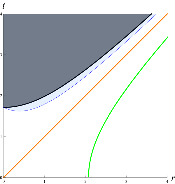
accompanied by a curvature singularity in spacetime. Moreover, a region of trapped surfaces appears around it, whose boundary forms an apparent horizon, as we shall see in the following. The curvature scalar diverges for , leading to eq. (12). This relation determines a surface on which the geometry collapses, as is apparent from eq. (11). The singularity has a natural interpretation as a generalization of the known ‘AdS crunch’, associated with dynamical fields in AdS spacetime Coleman; Higgstory, to a case in which the negative vacuum energy is not constant. The spacetime is well defined only in the regions in which . In the left plot of fig. 1 we depict the location of the singularity as a thick black line on the plane for , . This line asymptotically converges to the line .
The presence of the singularity also leads to the appearance of a region of trapped surfaces, whose boundary defines an apparent horizon. Outgoing/ingoing null geodesics, denoted by , define surfaces of areal radii . A truly outgoing geodesic results in the growth of the area of such a surface, while an ingoing geodesic results in the reduction of the area. On an apparent horizon, the rate of change of the area vanishes. The product
| (13) |
is a convenient quantity in order to search for a horizon. An apparent horizon would appear at the point where vanishes and subsequently changes sign. In our model, outgoing/ingoing geodesics for the metric of eq. (11) satisfy , while the areal radius is . This gives
| (14) |
with the subscripts denoting derivatives. In fig. 1 we depict as a blue line the location of the apparent horizon on which vanishes. The highlighted region between the apparent horizon and the singularity is the region of trapped surfaces.
The lightcone of an observer at the centre of the instanton, which corresponds to , is depicted as a thick red line in fig. 1. This surface delineates a region from which light cannot escape. Light rays travel at 45o towards the right (outgoing) or the left (ingoing). When they are emitted from any point above the red line, they always end up on the singularity. Based on this property, this surface can be characterized as an event horizon. Notice that the event horizon appears already at , before the emergence of trapped surfaces, as expected.
The bubble of true vacuum does not have a sharp surface separating it from the bulk space where the field asymptotically approaches the false vacuum at . One can use as a measure of the size of the bubble the radius at which the field has a value equal to a fraction of its initial value at the center . In fig. 1 we depict as a green line the location of this radius for and . It is apparent that the radius grows with a speed that asymptotically approaches that of light.
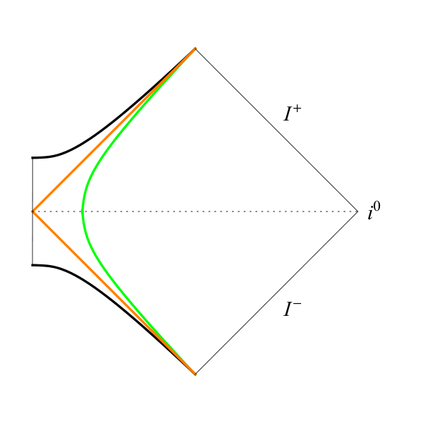
The combined picture that emerges is of a spherical bubble of true vacuum that expands asymptotically at the speed of light. A singularity appears in its interior that also expands asymptotically at the speed of light, surrounded by a region of trapped surfaces whose boundary forms an apparent horizon. The singularity and the bubble exterior are separated by an event horizon that coincides with the light cone of the observer at the centre of the instanton. At finite times, as measured by an asymptotic observer, the singularity is confined behind the horizon. However, the expansion of the bubble surface is not stopped by the collapse of its interior. At asymptotically late times the bubble eats up the entire false vacuum, while its interior is swallowed by the singularity. The picture is consistent with the analysis of Higgstory; Repeat for the Higgs potential.
The spacetime can also be depicted through a conformal diagram, shown in the right plot of fig. 1. In this diagram the time coordinate was allowed to take negative values. The bubble surface starts with infinite radius at , moves to a finite radius at , and subsequently expands again. The left plot corresponds to the upper half of the right plot. It is also apparent that both the ‘crunch’ and the bubble surface reach the future null infinity at the same point, swallowing the entire false vacuum. The conformal diagram is reminiscent of that of a Schwarzschild black hole. However, there is a a crucial difference: the singularity appears not at a single point, but on an entire spatial surface, similarly to the Big Bang singularity. In this sense, the event horizon is a cosmological horizon.
III Exact solutions in asymptotically de Sitter space
In this section we generalize the previous solutions to the case that the false vacuum has nonzero vacuum energy. Of particular interest is the case of positive energy density, as the resulting solutions describe tunnelling in de Sitter spacetime, a situation relevant for inflation. (Similar solutions have been derived for tunnelling from an AdS false vacuum, with an interepretation in the context of the AdS/CFT correspondence. See ads1; ads2 and references therein.)
For a conformally coupled scalar field () it is possible to find an exact solution for the potential
| (15) |
with . It describes Euclidean dS space of curvature , in coordinates such that the metric takes the form
| (16) |
where is the identity matrix. The field is given by the relation
| (17) |
and arbitrary . The action attributed to this configuration can be computed as
| (18) |
It is again given by eq. (4).
A peculiarity of the Euclidean solution (17) is that for the field does not reach zero. In this sense the configuration does not start exactly from the false vacuum. As discussed in detail in EWeinberg this is a typical occurrence in tunnelling from a dS vacuum, which can be considered as a thermal environment at the characteristic dS temperature. The field can be viewed as being thermally excited to a value away from the unstable minimum of the potential, with the tunnelling occuring subsequently from that value. It must be noted that a consistent picture requires that we assume the hierarchy , so that the bubble is nucleated with a surface well within the dS horizon. The asymptotic field value is then suppressed by . Also, realistic potentials include small modifications near the origin, which generate a locally stable false vacuum at vanishing field. These modifications induce only small corrections to the leading tunnelling solution (17), while forcing the field to approach a value close to zero for . Their main effect is to select a specific value for for the unique instanton solution.
The conformal transformation (7) and the field redefinition (8) generate a solution for a theory of a scalar field with a canonical kinetic term and a minimal coupling to gravity (). The potential is given by
| (19) |
The solution of the eom for a Lorentzian signature is
| (20) | |||||
| (21) |
The continuation to Euclidean signature provides an -symmetric solution of the eom resulting from the action (6) with and a potential given by eq. (19). Similarly to above, the field does not reach zero for . This is reflected in the fact that the curvature becomes
| (22) |
in this limit. Our assumptions that and that additional small modifications to the potential around the origin generate a minimum at this point imply that asymptotically the field will approach a value close to zero, while keeping the basic form of eqs. (20), (21). The main effect is that the solution will exist only for a specific value of .
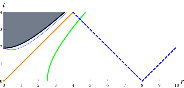
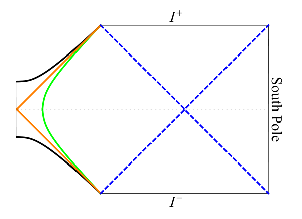
The geometry described by the metric (21) is depicted in fig. 2. The location of the ‘crunch’ singularity (thick black line), the region of trapped surfaces (light-blue shaded area), the apparent horizon (blue line), the event horizon (red line) and the location of the bubble surface (green line) are very similar, with small quantitative diffences, to those of fig. 1. The main difference between the two figures lies in the presence of the horizons of the asymptotic dS spacetime. These are depicted as dashed blue lines. It important to notice that the metric (21) can be written as the dS metric multiplied by a conformal factor. Therefore, it retains the causal structure of the dS geometry, apart from the region affected by the singularity of the conformal factor. As a result, the dS horizons are expected to persist as horizons of the full geometry, even though the bubble interior must be viewed as a quasi-AdS spacetime.
The location of the dS horizons can be determined by changing from the coordinates of the metric (21) with to Kruskal coordinates. In this way, one finds that the horizons correspond to the lines , depicted in fig. 1. These lines denote the limits for the information exchange with the observer on the South pole of the dS spacetime. Notice that, in the left plot of fig. 2, has not been taken much larger than in order for the details of the plot to be visible. Around the surface of the bubble, the geometry switches from quasi-dS to quasi-AdS. An extension of the solution to negative values of allows the construction of the conformal diagram, shown in the right plot of fig. 2 for .
There are three interesting points that can be deduced from fig. 2.
- •
- •
The second observation is that when the ‘crunch’ and the bubble surface reach the future null infinity a portion of space remains outside the bubble, so that a part of the false vacuum survives. Of course, after the end of inflation the relevant conformal diagram is that of fig. 1, which implies that the whole of the false vacuum is eventually swallowed by the ‘crunch’.
- •
Finally, the similarity of the right plot with the conformal diagram of the dS-Schwarzschild geometry is apparent. However, there is a crucial difference in that the singularity appears not at a point, but on a whole spatial surface, similarly to the Big Bang singularity. As a result, the event horizon depicted by the red line is a cosmological horizon.
IV Numerical solutions for a class of models
The purpose of this work was to derive analytical solutions of vacuum decay in unbounded potentials in order to understand in precise terms the effect on the bubble surface of the ‘crunch’ developing within the nucleated quasi-AdS bubble interior. Exact solutions were derived for specific potentials, which demonstrated that the surface of a sufficiently large bubble keeps expanding, independently of the ‘rolling’ of the field down the potential and the appearance of a singularity. The results complement the numerical analysis of Repeat and reconfirm the general picture presented in Higgstory.
A variety of other models can be constructed in an implicit fashion, resulting in very similar solutions and conformal diagrams. It was observed in Apostolopoulos that a conformally flat metric of the form , with , and a scalar field configuration obeying
| (23) |
satisfy the Einstein equations for a minimally coupled scalar theory with a potential given implicitly as
| (24) |
This allows the construction of models directly in the Einstein frame by selecting the desired , solving eq. (23) for , inverting this function and deriving the function through substitution in eq. (24). Even though finding analytical solutions is not easy, a numerical implementation of the above procedure is straightforward. An interesting class of solutions has metrics of the form
| (25) |
with an integer larger than 2. The metric is similar to (21). It includes one conformal factor that corresponds to an exact dS spacetime and another that induces a ‘crunch’ singularity. For the dS metric is approached in the limit faster than in the case of the metric (21).
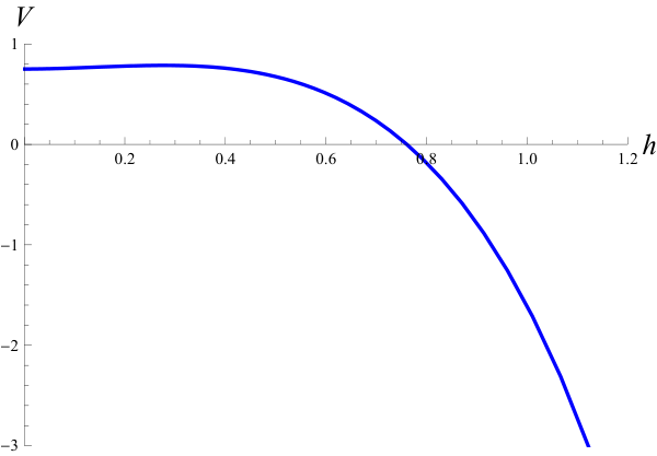
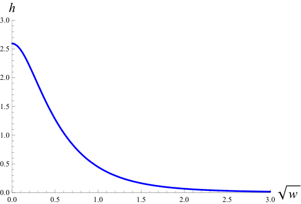
The solution of eq. (23) describes a field that vanishes for . The resulting configuration for an Euclidean signature describes an instanton that drives the tunnelling from the false vacuum at the origin to the unstable region of the potential. This configuration is depicted in the right plot of fig. 3 as a function of . The potential is given implicitly through eq. (24) and is depicted in the left plot of fig. 3. It has a shallow minimum at the origin, separated by a barrier from the large-field region where it becomes unbounded from below. This numerical solution confirms the validity of the discussion in the previous section and refs. Higgstory; Repeat. The bubble expands continuously, despite the appearance of the ‘crunch’ in its interior, crosses the horizon of the external dS geometry, and eventually reaches asymptotic null infinity.
Acknowledgments
I would like to thank P. Apostolopoulos, C. Charmousis, I. Papadimitriou, A. Strumia and R. Troncoso for useful discussions. The research of N. Tetradis was supported by the Hellenic Foundation for Research and Innovation (H.F.R.I.) under the “First Call for H.F.R.I. Research Projects to support Faculty members and Researchers and the procurement of high-cost research equipment grant” (Project Number: 824).
References
- (1) J. R. Espinosa, G. F. Giudice, E. Morgante, A. Riotto, L. Senatore, A. Strumia and N. Tetradis, JHEP 09 (2015), 174 [arXiv:1505.04825 [hep-ph]].
- (2) A. Strumia and N. Tetradis, JHEP 09 (2022), 203 [arXiv:2207.00299 [hep-ph]].
- (3) J. Elias-Miro, J. R. Espinosa, G. F. Giudice, G. Isidori, A. Riotto and A. Strumia, Phys. Lett. B 709 (2012), 222-228 [arXiv:1112.3022 [hep-ph]].
- (4) D. Buttazzo, G. Degrassi, P. P. Giardino, G. F. Giudice, F. Sala, A. Salvio and A. Strumia, JHEP 12 (2013), 089 [arXiv:1307.3536 [hep-ph]].
- (5) A. V. Bednyakov, B. A. Kniehl, A. F. Pikelner and O. L. Veretin, Phys. Rev. Lett. 115 (2015) no.20, 201802 [arXiv:1507.08833 [hep-ph]].
- (6) O. Lebedev and A. Westphal, Phys. Lett. B 719 (2013), 415-418 [arXiv:1210.6987 [hep-ph]].
- (7) A. Kobakhidze and A. Spencer-Smith, Phys. Lett. B 722 (2013), 130-134 [arXiv:1301.2846 [hep-ph]].
- (8) J. Kearney, H. Yoo and K. M. Zurek, Phys. Rev. D 91 (2015) no.12, 123537 [arXiv:1503.05193 [hep-th]].
- (9) M. Kawasaki, K. Mukaida and T. T. Yanagida, Phys. Rev. D 94 (2016) no.6, 063509 [arXiv:1605.04974 [hep-ph]].
- (10) A. Rajantie and S. Stopyra, Phys. Rev. D 95 (2017) no.2, 025008 [arXiv:1606.00849 [hep-th]].
- (11) A. Salvio, A. Strumia, N. Tetradis and A. Urbano, JHEP 09 (2016), 054 [arXiv:1608.02555 [hep-ph]].
- (12) K. Enqvist, M. Karciauskas, O. Lebedev, S. Rusak and M. Zatta, JCAP 11 (2016), 025 [arXiv:1608.08848 [hep-ph]].
- (13) A. Joti, A. Katsis, D. Loupas, A. Salvio, A. Strumia, N. Tetradis and A. Urbano, JHEP 07 (2017), 058 [arXiv:1706.00792 [hep-ph]].
- (14) T. Markkanen, A. Rajantie and S. Stopyra, Front. Astron. Space Sci. 5 (2018), 40 [arXiv:1809.06923 [astro-ph.CO]].
- (15) A. Mantziris, T. Markkanen and A. Rajantie, JCAP 03 (2021), 077 [arXiv:2011.03763 [astro-ph.CO]].
- (16) S. R. Coleman and F. De Luccia, Phys. Rev. D 21 (1980), 3305.
- (17) V. De Luca, A. Kehagias and A. Riotto, JCAP 09 (2022), 055 [arXiv:2205.10240 [hep-ph]].
- (18) A. R. Brown and E. J. Weinberg, Phys. Rev. D 76 (2007), 064003 [arXiv:0706.1573 [hep-th]].
- (19) S. Fubini, Nuovo Cim. A 34 (1976), 521.
- (20) X. Dong and D. Harlow, JCAP 11 (2011), 044 [arXiv:1109.0011 [hep-th]].
- (21) S. Kanno and J. Soda, Int. J. Mod. Phys. D 21 (2012), 1250040 [arXiv:1111.0720 [hep-th]].
- (22) S. Kanno, M. Sasaki and J. Soda, Class. Quant. Grav. 29 (2012), 075010 [arXiv:1201.2272 [hep-th]].
- (23) J. R. Espinosa, JCAP 06 (2020), 052 [arXiv:2003.06219 [hep-ph]].
- (24) J. R. Espinosa, J. F. Fortin and J. Huertas, Phys. Rev. D 104 (2021) no.6, 065007 [arXiv:2106.15505 [hep-th]]
- (25) S. de Haro, I. Papadimitriou and A. C. Petkou, Phys. Rev. Lett. 98 (2007), 231601 [arXiv:hep-th/0611315 [hep-th]].
- (26) I. Papadimitriou, JHEP 05 (2007), 075 [arXiv:hep-th/0703152 [hep-th]].
- (27) W. Israel, Nuovo Cim. B 44S10 (1966), 1 [erratum: Nuovo Cim. B 48 (1967), 463].
- (28) P. S. Apostolopoulos, [arXiv:2211.01084 [gr-qc]].