Estimating the Instantaneous Reproduction Number With Imperfect Data: A Method to Account for Case-Reporting Variation and Serial Interval Uncertainty
Abstract
During an infectious disease outbreak, public health decision-makers require real-time monitoring of disease transmission to respond quickly and intelligently. In these settings, a key measure of transmission is the instantaneous time-varying reproduction number, . Estimation of this number using a Time-Since-Infection model relies on case-notification data and the distribution of the serial interval on the target population. However, in practice, case-notification data may contain measurement error due to variation in case reporting while available serial interval estimates may come from studies on non-representative populations.
We propose a new data-driven method that accounts for particular forms of case-reporting measurement error and can incorporate multiple partially representative serial interval estimates into the transmission estimation process. In addition, we provide practical tools for automatically identifying measurement error patterns and determining when measurement error may not be adequately accounted for. We illustrate the potential bias undertaken by methods that ignore these practical concerns through a variety of simulated outbreaks. We then demonstrate the use of our method on data from the COVID-19 pandemic to estimate transmission and explore the relationships between social distancing, temperature, and transmission.
Keywords Bayesian COVID-19 Infectious Disease
1 Introduction
During infectious disease outbreaks, decision-makers require timely, accurate monitoring of disease transmission to inform public health responses. An important quantity for infectious disease surveillance is the reproduction number, , which is defined as the average number of secondary cases generated by an infected individual over his or her infectious period. As demonstrated during the recent COVID-19 pandemic, the quantity has many uses including to monitor and project the spread of disease in a particular region (Wang et al. 2020; Chen et al. 2020; Wu et al. 2020), parameterize models that evaluate intervention efficacy (Pan et al. 2020; Jorge et al. 2021; Zhang et al. 2021; Peng et al. 2020), and provide insights into factors associated with transmission (Rubin et al. 2020; Wang and Teunis 2020). When real-time monitoring is a priority, Fraser 2007 and Gostic et al. 2020 recommend estimating the time-varying instantaneous reproduction number, , which represents the average number of secondary cases that an individual infected at time could expect to infect should current conditions persist.
Numerous statistical methods have been developed to estimate the reproduction number using the Time-Since-Infection (TSI) epidemiological model (Kermack and McKendrick 1927), with many summarized in White et al. 2021. When estimating time-varying reproduction numbers, methodologists have largely favored Bayesian approaches due to complex likelihoods induced in the time-varying setting (Cauchemez et al. 2006; Cori et al. 2013; Thompson et al. 2019; Quick et al. 2021a). In particular, Cori et al. 2013’s development of an estimator for has been widely used in practice, including during the COVID-19 pandemic.
Despite the success of widely-used methodology, TSI models inherently rely on case-notification data, which is known to contain measurement error due to variation in case-reporting (Gostic et al. 2020; Ricon-Becker et al. 2020; Bergman et al. 2020). High reporting variation often renders estimates too volatile for practical use. In these settings, practitioners commonly aggregate case counts or transmission estimates over a sliding window of pre-determined length (Gostic et al. 2020). However, these smoothing techniques are not targeted to reporting patterns and therefore may smooth over relevant signals in the data. Previous methods have addressed limitations in case ascertainment when additional seroprevalance (Quick et al. 2021a) or hospitalization data (White et al. 2009) are available and accurate. Shi et al. 2022 develop a flexible approach that allows for uncertainty in transmission estimates not accounted for in a predictive time-series model, which may result in part from case reporting patterns, but do not directly target nuisance reporting signals in the observed data.
In addition to case-notification data, TSI models require an estimate for the distribution of the serial interval, which is defined as the time between case definitions of infector-infected pairs. Particularly early in an outbreak, serial interval estimates may come from small studies on a particular subpopulation, often close to the outbreak source. However, prior work has found significant heterogeneity in serial intervals across many factors including region (Rai et al. 2021, Alene et al. 2021) and age (McAloon et al. 2021). Therefore, a single serial interval study is likely representative of only a fraction of the target population. Researchers have tried to address this limitation by allowing for additional uncertainty of this parameter in their models. Cori et al. 2013 allowed for serial interval uncertainty with a grid-sampling approach over a user-specified range of serial interval means and variances. Thompson et al. 2019 improved upon this approach with a two-step process that first estimates the posterior distribution of the serial interval using known pairs of index and secondary cases and then uses this posterior distribution to estimate , but relies on representative and accurate contact tracing data.
Here, we propose a unified framework to robustly estimate in the presence of case reporting measurement error and non-representative serial interval studies without additional contact tracing, seroprevalence, or hospitalization data. Our Bayesian framework joins together a model of case-reporting patterns to address measurement error, a mixture model to incorporate multiple serial interval distributions, and an autoregressive transmission model that dually serves to increase statistical power and identify factors associated with transmission. To assist practitioners, we additionally provide an algorithm to identify weekly reporting patterns and an objective test to determine when pre-analysis case-smoothing may be favorable to a measurement error model.
The remainder of the paper is organized as follows: In Section 2, we first describe the TSI model before introducing our proposed model. In Section 3, we present numerical studies across a variety of simulated outbreaks to empirically demonstrate the added capabilities of our proposed approach. We then apply our methodology to study the United States COVID-19 outbreak in 2020 to estimate transmission and understand transmission risk factors in Section 4. Finally, we summarize our findings and discuss further methodological considerations in Section 5.
2 Methods
2.1 Time-Since-Infection Model
We first briefly review the foundations of TSI model estimators for as described in Fraser 2007. Let denote the number of incident infections generated on day and be the infectiousness on day for an individual that was infected days ago. The possible generators of are the previously infected individuals: , where an individual infected on day generates, on average, new infections on day . We can then specify as a function of and through the so-called renewal equation:
| (1) |
where denotes the number of days at which infectivity is considered no longer viable. Assuming that the generation interval distribution, , defined as the proportion of total infections generated by an infected individual that are generated on day since infection, is independent of calendar time, , we can decompose as:
| (3) |
In practice, we do not observe the true generation interval or infections, leading to probabilistic methods that allow for uncertainty in this relationship.
2.2 A Bayesian Model in the Presence of Case Reporting Measurement Error and Serial Interval Distribution Uncertainty
Consider observing a time-series of reported cases on day of outbreak , , which are a proxy of the true latent incident cases, , where . The observed and latent cases differ due to reporting patterns that are consistent within reporting periods, (e.g., day-of-week). We observe a vector of time-varying covariates, , associated with the latent instantaneous reproduction number on day , . Finally, we observe external serial interval distribution estimates, (), included to represent at least part of the target population.
Then, we specify our model over the joint data distribution hierarchically as:
| (4) | ||||
| (5) | ||||
| (6) | ||||
| (7) |
In the first layer of our model, we specify that the observed reported cases, , are centered around the scaled latent true incident cases, where the scaling weights, , are specific to the reporting period of day , .
We then link incident cases to by extending the TSI model to incorporate a mixture of serial interval distribution estimates, . Here, are unknown mixture weights that allow for uncertainty in the representativeness of available estimates.
We propose modeling according to the generalized autoregressive moving average model (GARMA) derived in Benjamin et al. 2003 for a Gamma distribution with autoregressive order and moving average order . Setting , this model specifies:
where and denote the unknown covariate-effect and autoregressive parameters, respectively. By incorporating an autoregressive model for , we can improve the stability and power of our estimates in a statistically-principled manner, while also enabling the exploration of associations between predictors and transmission (Shi et al. 2022).
We define for compactness, where these are drawn from a distribution composed of generally noninformative independent priors according to hyper-parameters .
2.3 Determining the Case Reporting Measurement Error Model
Realistically, practitioners may have to identify the mapping in (4) that partitions day-of-outbreak into reporting periods themselves. An ideal mapping captures all variation in cases due to reporting patterns and none of the variation in cases due to important transmission signals. Here, we propose developing a mapping based on day-of-week patterns, which are highly associated with reported case counts and appear likely to persist in future outbreaks (Ricon-Becker et al. 2020; Bergman et al. 2020). While relevant transmission factors like increased socialization on weekends may explain some of the day-of-week patterns, we can incorporate social distancing metrics into (6) to capture the relevant components of these signals.
When model parsimony is important (e.g., shorter length studies), we propose the following algorithm to automatically partition the days of the week into periods of relatively homogeneous reporting patterns:
Intuitively, Algorithm 1 first identifies general temporal trends in cases (Line 2), which allows us to then separate out the day-of-week patterns (Line 3) using standard time-series decompositions (Hyndman and Athanasopoulos 2018). We then cluster the days of the week (Line 6) according to a vector of their relative reporting variation (Line 4). With each size- clustering, we regress the reporting variations on cluster-specific intercepts to test how well the clustering explains the reporting variation (Line 7). Finally, we select a parsimonious clustering of the days of week according to the Akaike Information Criterion (AIC) (Line 9), which gives us our mapping (Line 10). A visualization of this method using COVID-19 data from New York is provided in Figure A1.
The estimated cluster-specific coefficients (Line 11) provide reasonable informative priors for the reporting weights, , if desired. A perhaps more important consideration for the priors on these weights is the choice in prior distribution, which may enforce certain constraints as discussed further in Section A1. In practice, we constrain the mean of the weights to be equal to one through a Dirichlet prior.
In certain settings, the day-of-week measurement error model may not sufficiently separate reporting patterns from transmission signals, like when reporting patterns change over time and are correlated with . In lieu of an alternative sufficient model, it may be necessary for practical utility to instead reduce measurement error with a more coarse smoothing technique, like by taking rolling averages of case data prior to analysis (Gostic et al. 2020). Whereas the method of Cori et al. 2013 uses window-based techniques to smooth estimates, we choose to smooth reported cases to more directly target case reporting measurement error. Since coarse smoothing approaches may smooth over relevant transmission signals, we suggest pre-analysis case-smoothing only when it provides a substantial improvement to the volatility of estimates, . If using the day-of-week measurement error model is substantially more volatile than when using case-smoothing, then it is likely that using the day-of-week measurement error model is too volatile to be useful. We measure volatility via lag-one auto-correlation, which estimates the correlation between and across , and ranges between -1 (high volatility) to +1 (low volatility). To make the decision between measurement error approaches objectively in our work, we derive confidence intervals for the lag-one auto-correlation of the time-series from the measurement error model approach using corrected Pearson coefficient variances (Afyouni et al. 2019) and only select the case-smoothing method when the lag-one auto-correlation of time-series from the case-smoothing approach falls above the upper confidence bound.
3 Simulation Studies
3.1 Design
We designed our simulations to mimic the noted imperfections in available real-world data gathered from disease outbreaks. We simulated outbreaks across a variety of realistic trend patterns (TPs), which specify how transmission changes over the outbreak period. These temporal patterns corresponded to three intuitive phases: an unrestricted growth phase representing a period of high transmission (e.g., minimal public response), a lockdown phase where transmission decreases (e.g., high public response), and an equilibrium phase where balance occurs between the virus and public responses.
TP1 outbreaks followed an unrestricted-lockdown-equilibrium paradigm, whereas TP2 outbreaks followed an unrestricted-lockdown-unrestricted-lockdown-equilibrium transmission paradigm. In TP3 outbreaks, transmission transitioned smoothly from unrestricted to equilibrium. These transmission patterns were generated by simulating:
where , , . is designed to align with the daily visitation difference social distancing measure described further in Section 4.
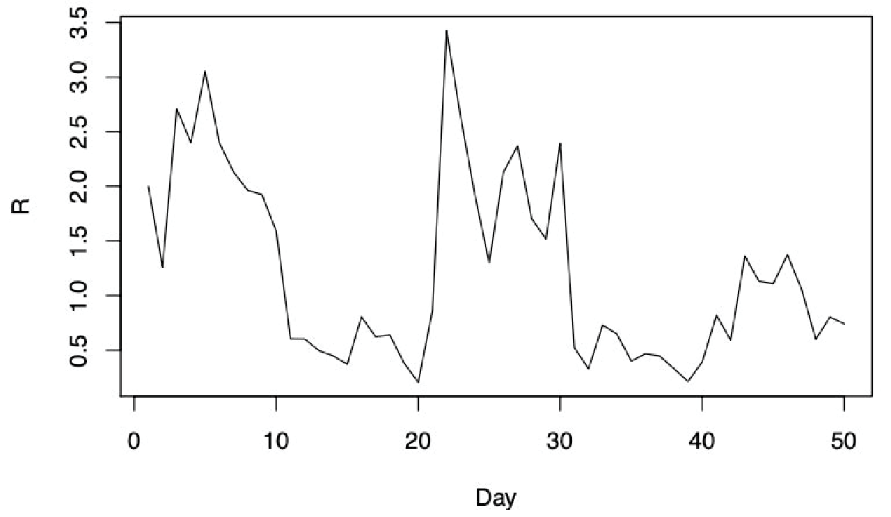
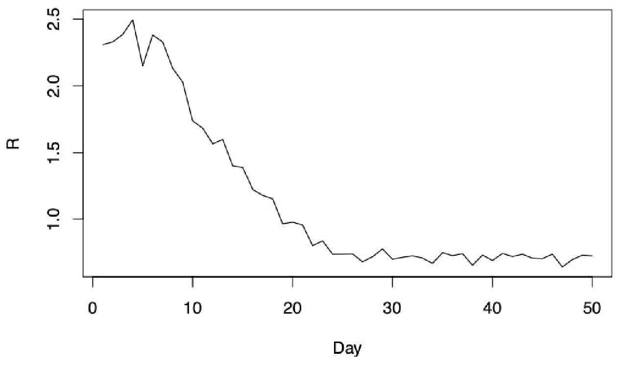
After specifying , , and parameters, we then sequentially simulated according to (6), according to (5), and according to (4). Here, generally mapped day-of-outbreak to period-of-week clusters - , , . Specified parameters for and can be found in Section A2. Examples of simulated time-series by trend pattern are visualized in Figure A2.
In addition to outbreak TPs, we also differed simulations by data scenarios (DSs), which represent different nuances in the observed data and are summarized in Table 1. In DS0, we generated data with no variation in case reporting (), a single (correctly-specified) serial interval distribution (, ), and provided our model an uninformative observed covariate (). Therefore, our proposed model only extends the method of Cori et al. 2013 by including a misspecified model for (6). In each sub-scenario of DS1, we added a single nuance to the observed data – (A) multiple serial interval interval estimates are available (), (B) the true data-generating mechanism covariate is observed (), and (C) observed reported cases contain measurement error ().
DS2 combines all three nuances of DS1, while simulating from the parametric distributions specified in our model (DS2A) and alternative distributions (DS2B). In the latter, we violated the parametric assumptions in (4), (5), and (6) by generating , , and from Log-Normal (rounded), Negative Binomial, and Log-Normal distributions, respectively.
| Data | Reporting | Serial | Predictors | Parametric |
|---|---|---|---|---|
| Scenario | Variation | Interval | Specified | Specification |
| 0 | Null | Given | No | Correct |
| 1A | Null | Uncertain | No | Correct |
| 1B | Null | Given | Yes | Correct |
| 1C | Correctly Specified | Given | No | Correct |
| 2A | Correctly Specified | Uncertain | Yes | Correct |
| 2B | Correctly Specified | Uncertain | Yes | Misspecified |
| 3A,B | Misspecified | Uncertain | Yes | Correct |
| 3C | Misspecified | Given | Yes | Correct |
In each sub-scenario of DS3, we generated observed case data to violate a different assumption of our measurement error model – (A) reporting patterns stop halfway through the outbreak (), violating our time-invariant assumption on and (B) reporting weights do not have mean 1 (), violating the Dirichlet prior we impose on . In DS3C, reporting patterns cannot be separated from transmission signals as case reporting alternates between low reporting on odd days and high reporting on the following day (intuitively to catch up), does not have mean 1 weights, and is correlated with . We implemented this by setting , in the unrestricted phase, in the lockdown phase, and in the equilibrium phase.
3.2 Implementation
For DS0-DS3B, we generated short simulations (50 days) for all trend patterns and long simulations (100 days) for TP2. For DS3C, we only generated short simulations for TP1. We conducted 1200 simulations for each scenario-trend pattern pair and discarded simulations with low case counts () for more than of days as these generally indicated outbreaks that did not persist for the entire study length. On average, a scenario-context pair resulted in 989 and 804 kept simulations for short and long runs, respectively.
We evaluated the relative performance of and 95% credible intervals from our proposed method and the method of Cori et al. 2013 (Baseline) using Mean Squared Error (MSE), Mean Raw Bias (Bias), and coverage probability. For MSE and Bias, we first scaled the difference between estimated and true values by the true parameter value. We did not consider the first 7 days of estimates to restrict model comparisons to estimates with sufficient case data.
We implemented the proposed model with JAGS (Plummer 2003) to develop a Markov Chain Monte Carlo (MCMC) sampler with 8 chains, 2000 burn-in iterations and 4000 total iterations per chain, and a thinning parameter of 2. We used the posterior mean for point estimates of parameters and estimated credible intervals using the and percentiles of the posterior samples. We implemented the baseline method with the EpiEstim R package (Cori 2021) and input the mean of the available serial interval estimates in data scenarios where the correct serial interval was not considered given (DS1A, DS2A-DS3B).
3.3 Results
We first compared the performance of baseline method implementations according to the window size, or bandwidth, parameter () and specification of serial interval uncertainty (U) to select an appropriate comparison to our method. We centered windows at (i.e., window=) to estimate , since these resulted in estimates most aligned with the true .
Results from the , , and models are summarized in Table A1. The choice in , which controls the smoothness of as visualized in Figure A3(a), drastically altered model performance depending on which assumptions hold. In DS0-DS1B, models with performed best in terms of MSE, bias, and coverage probability since they do not smooth over the signals in case data, which are largely relevant in these simple scenarios. However, smoothing with resulted in comparable (DS2A-DS3B) and even improved (DS3C) estimates in more complex settings when reporting patterns induced large amounts of noise in case data. The approach of the baseline method to address serial interval uncertainty (U) improved coverage probability in our simulations but drastically increased MSE and Bias of . The low point estimation accuracy for this approach is likely influenced by the disconcordance between the true serial interval distribution form (max 4 days, non-parametrically distributed) and the assumed form of the method (max 20 days, Gamma distributed). Therefore, we focused on the baseline model with and serial interval distribution uncertainty ignored, since this window size is most similar in spirit to our attempt to capture granular signals in and this implementation had the best performance for a majority of scenarios.
Comparison between Proposed and Baseline Methods with Specified Reporting Periods
| Data | MSE (x) | Bias () | Coverage Probability () | |||
|---|---|---|---|---|---|---|
| Scenario | Propose | Relative Change () | Proposed | Relative Change () | Proposed | Baseline |
| 0 | 1.29 | -10.4 | 1.88 | -6.5 | 94.97 | 95.13 |
| 1A | 1.48 | -43.5 | 2.04 | +5.7 | 95.41 | 70.65 |
| 1B | 1.36 | -34.0 | 2.42 | -24.4 | 94.88 | 95.07 |
| 1C | 3.78 | -91.0 | 3.57 | -65.5 | 90.91 | 16.86 |
| 2A | 4.08 | -89.6 | 4.88 | -51.9 | 91.78 | 19.80 |
| 2B | 11.99 | -77.3 | 1.63 | -80.4 | 59.93 | 16.25 |
| 3A | 10.43 | -57.3 | 6.77 | +19.0 | 70.25 | 37.85 |
| 3B | 3.79 | -87.8 | 4.97 | -42.3 | 92.92 | 22.61 |
| 3C | 212.89 | -21.8 | 69.43 | -11.3 | 0.65 | 0.72 |
Performance metrics for comparing the proposed method with a pre-specified to the selected baseline method are summarized in Table 2. The proposed model showed almost uniformly superior MSE, bias, and coverage probability than the baseline method in these scenarios.
In DS0-DS1B, our proposed model demonstrated improvement over the baseline method in terms of MSE (10.4-43.5% reduction) and bias (6.5-24.4% reduction), except for bias in DS1A (5.7% higher), provided that we correctly ignore case reporting measurement error. Interestingly, we saw slight improvement from the baseline method in DS0 when our autoregressive model was over-specified, which speaks to the predictive power of autoregressive models in general. Coverage probabilities were near the nominal rate for both methods in these scenarios except for the baseline method in DS1A (70.7% coverage), demonstrating the improvement in uncertainty quantification using our method when the true serial interval is a mixture of available serial interval estimates. The improvement in relative performance of the proposed method between DS0 and DS1B (10.4 to 34.0% lower MSE, 6.5 to 24.4% lower bias) suggests a benefit to modeling with informative covariates in the estimation process.
When we introduced measurement error in case reporting in DS1C, we saw clear benefits of correctly modeling these patterns (91.0% reduction in MSE, 65.5% reduction in bias, and 74.05% more coverage probability). These results are comparable to those in DS2A, implying a high relative importance of the measurement error model in our simulations. Figure A3(b) provides an example fit for both the proposed and baseline methods from DS2A. When we violated the parametric assumptions of our model in DS2B, we saw diminished performance in MSE and coverage probabilities, which we attribute largely to the inability of our specified Poisson distributions to handle over-dispersion induced by the true distributions.
In DS3A-DS3C, we explored robustness to misspecifications of the case reporting measurement error model. When we changed case reporting patterns over time in DS3A, we saw lessened benefits (57.3% lower MSE, 19.0% higher bias, 32.40% more coverage probability) since we specified a single for the entire outbreak period in our model. Meanwhile, the assumption of no case reporting measurement error in the baseline method is satisfied in the second half of these outbreaks. The similar results between DS2A and DS3B suggest that imposing a constraint on the mean of does not substantially reduce identification of , even when violated. We note that this observation likely results from the partial identifiability of , in that only the relative reporting weights, rather than the scale of , affect identification of , which we discuss further in Section A1. In DS3C, severe misspecification of the case reporting patterns induced substantial MSE and Bias for both methods. While this scenario is likely more extreme than would be seen in practice, it suggests the need for window-based smoothing techniques when the case reporting pattern is not well identified. Figure A3(c) provides a visual example of this scenario.
Performance of Methods to Determine the Case Reporting Measurement Error Model
| Clustering Accuracy | Case-Smoothing | Accuracy | ||||
| Data | WFM | WFM | Smoothing | MSE | Bias | Cov. Prob. |
| Scenario | (Short) | (Long) | Selected () | ( | () | () |
| 0 | 85.8 | 84.5 | 0.2 | 6.17 | 7.72 | 89.40 |
| 1A | 79.6 | 81.2 | 2.6 | 6.67 | 8.74 | 89.50 |
| 1B | 85.2 | 84.0 | 0.0 | 4.14 | 7.61 | 91.34 |
| 1C | 57.8 | 77.0 | 0.1 | 11.23 | 8.34 | 69.14 |
| 2A | 58.7 | 77.0 | 0.2 | 10.48 | 10.60 | 72.04 |
| 2B | 66.0 | 83.0 | 3.3 | 14.19 | 3.10 | 57.02 |
| 3A | – | – | 1.0 | 17.21 | 13.40 | 56.55 |
| 3B | 50.5 | 73.9 | 0.2 | 9.91 | 10.91 | 71.19 |
| 3C | – | – | 100.0 | 18.51 | 8.78 | 23.49 |
– Reporting patterns vary over time so performance metrics are not calculated
We also evaluated the performance of Algorithm 1 in identifying the correct case reporting periods and our proposed case-smoothing decision tool in selecting an appropriate approach to address measurement error in case reporting.
To assess the performance of Algorithm 1, we computed a weighted f-measure (WFM) metric, which is a clustering metric ranging between 0 and 1 that looks at all pairwise combinations of the days of the week and penalizes pairs that are incorrectly clustered together (restrictive error) twice as much as those incorrectly mapped separately (parsimony error). To assess the performance of our case-smoothing decision tool, we looked at the percentage of simulations that the tool selects case-smoothing in favor of the measurement error model in settings where we prefer the former (DS3C) and the latter (DS0-DS3B). Finally, we assessed the joint performance of our model, algorithm, and decision tool in estimating to understand realistic method performance in practical settings. These metrics are summarized by data scenario in Table 3.
Example WFM scores are provided in Table A2 for context. In DS0-DS1B when all days of the week should be mapped to the same cluster, the average WFM scores are between 79.6-85.8 for both short and long runs, suggesting 1-2 parsimony mistakes on average. In DS1C-DS2B and DS3B, the average WFM scores are between 50.5-66.0 for short runs, suggesting one restrictive mistake and one parsimony mistake on average. These improve to WFM scores of 73.9-83.0 in long runs, suggesting higher accuracy with longer time-series if the reporting patterns are consistent over time.
In settings with identifiable measurement error (DS0-DS3B), we would prefer to model the measurement error approach rather than smooth over it. This preference holds even in settings where there is no measurement error (DS0-DS1B), since is within the solution set of our model. In settings when measurement error in case-reporting cannot be separated from transmission signals (DS3C), we would prefer to reduce measurement error with the case-smoothing approach. Our decision tool works well in our simulations and rarely selected the case-smoothing approach in DS0-DS3B (0.0-3.3%) but always did in DS3C.
Finally, estimates of when reporting periods are estimated using Algorithm 1 and the measurement error approach is selected using the decision tool demonstrated improved stability across scenarios. Estimation of the reporting periods expectedly reduced estimate efficiency compared to when reporting periods were given a priori, particularly in simple scenarios. However, use of the decision tool greatly improved estimate accuracy in DS3C.
4 Analysis of COVID-19 outbreak
4.1 Study Design
We demonstrate the proposed method in practice using data from the COVID-19 pandemic. We collected reported cases and measures of social distancing and temperature from March 25, 2020 to November 10, 2020 (230 days) for 10 United States (US) counties that contain large metropolitan cities – Austin, Texas; Chicago, Illinois; Dallas, Texas; Houston, Texas; Los Angeles, California; Miami, Florida; New York, NY; San Diego, California; and San Francisco, California. Although data is collected at the county level, we refer to the major city of the county throughout this section. Our interests are twofold, as we wish to both estimate transmission and explore transmission dynamics, such as the role of social distancing and temperature on transmission.
We used daily visitation difference, which measures the relative change in visits to non-essential businesses from pre-pandemic times, and wet bulb temperature, which measures the complex thermodynamic relationship between temperature and humidity, as predictors of transmission. These variables, provided by Unacast and the National Ocean and Atmospheric Administration Local Climatological Data respectively, were previously found to be associated with transmission (Rubin et al. 2020). We used the average, standardized metrics from days as and included 4 lag terms () in our autoregressive transmission model.
In addition to county-specific data on reported cases and transmission factors, we selected serial interval distribution estimates from China (He et al. 2020), Ireland (McAloon et al. 2021), and a systematic review on the world population (Alene et al. 2021) as components of our serial interval mixture. The study by He et al. 2020 was used for a study on California counties (Worden et al. 2020), whereas the latter two provide comprehensive studies from different parts of Europe and Asia. The lack of available serial interval studies on a diverse US population highlights the practical challenges that practitioners often face when searching for a representative serial interval study. While some of these studies account for the possibility that a generated case is identified prior to that of the generator, we did not and instead adjusted their estimated serial interval distributions to maintain the relative densities over the positive support of the distribution. For the baseline method implementation, we used the average of these three serial interval estimates.
4.2 Transmission Estimation

We implemented methods as in Section 3, except we used 12K MCMC samples (6K burn-in) per chain to account for the larger parameter space of a 230-day study. We estimated reporting periods for each county using Algorithm 1 and selected an appropriate measurement error approach using the case-smoothing decision tool. Our decision tool selected pre-analysis case-smoothing for two of the counties (Houston and Austin) and the case reporting measurement error model for the other eight.
Figure 1 visualizes estimates from the proposed and baseline methods for both San Francisco and Los Angeles. Qualitatively, the proposed method produced smoother and more usable estimates than the baseline method. Importantly, this smoothing is conducted in a more principled fashion than window-based smoothing techniques since it directly targets nuisance reporting patterns.
While we suspect that much of the improved estimate smoothness results from the identification of case-reporting patterns, it may also result from increases in estimate stability brought on by our transmission predictor model and/or flexibility brought on by allowing deviation from a specified serial interval distribution. To the latter point, Figure 2 shows heterogeneity in serial interval distribution estimates for each county, suggesting that such variations enabled a better overall model fit. Interestingly, Texas and California had the most and least volatile estimates, respectively, which may suggest more identifiable reporting patterns in the latter.
4.3 Exploring Factors of Transmission

We explored the association of specified covariates and transmission by examining the coefficient estimates from our method, which are shown in Figure 3. The association between social distancing and transmission for San Diego and New York is demonstrated qualitatively in Figure 4. Each additional unit (county-specific standard deviation) of daily visitation difference is associated with an increase in expected . Thus, our estimates associate an increase of in expected per standard deviation increase in social distancing relative to pre-pandemic baselines. The confidence intervals for these associations do not include the null effect () except for San Francisco, which has highly volatile and often even positive daily visitation differences in the data.
Our estimates for the effect of wet bulb temperature showed a negative but inconclusive association with the transmission, which differs from previous studies that found significant negative associations (Rubin et al. 2020). The high correlation of temperature with the presumably stronger and offsetting social distancing measure () and the suspected non-linear relationship between temperature and transmission may partially explain the weakened association.


5 Discussion
When estimating , practitioners must use noisy case-notification data subject to reporting patterns and non-representative external serial interval estimates. In this work, we demonstrated the importance of modeling case reporting measurement error and accounting for serial interval uncertainty when estimating with imperfect data and proposed a method to do so. Our Bayesian framework shares information and uncertainty between intuitive modeling layers, allowing for informed but flexible parameter exploration. In our simulation studies, these benefits enabled more robust parameter and uncertainty estimates than methods that do not target these practical considerations. Further, our objective methods to determine the case reporting measurement error approach augment our proposed model and equip practitioners with tools to avoid ad-hoc smoothing selection techniques. We applied our framework to a study on the 2020 US COVID-19 outbreak to derive potentially more usable estimates. In addition to benefiting monitoring efforts, these estimates may better parameterize models that rely on as we avoid smoothing over relevant signals in the data. Finally, our framework allowed us to explore the association of transmission factors in explaining transmission, which suggested a large influence of social distancing on transmission.
Our framework targets measurement error due to case reporting and can be viewed as a new approach to smoothing, where our smoothing technique incorporates our knowledge of differential reporting behavior across days of the week. When day-of-week reporting variation does not sufficiently capture overall reporting variation, coarser methods like rolling averages or spline-smoothing may be beneficial. Our approach does not address unidentified cases, which result from factors like asymptomatic transmission and testing guidelines. When the rate of case-identification is constant over time, day-of-week reporting weights () are identifiable up to a constant and our estimates for are unbiased as this constant rate is canceled out in the renewal equation. However, estimates are biased if the identification rate changes over time (White and Pagano 2010) and while methods have been developed to use additional data sources to account for these concerns (White et al. 2009; Quick et al. 2021a), they come with their own assumptions about additional data and modeling layers (Dean and Yang 2021). Changes in reporting patterns may also trigger changes in the serial interval over time (Datta and Mukherjee 2021; Quick et al. 2021b). In addition to different sources of data, methods that integrate case data from multiple regions into the estimation process may provide benefits, but also come with substantial challenges.
While our approach provides insights relevant to future transmission and the effects of transmission factors, it is designed to estimate rather than to forecast future transmission or robustly analyze effects. Nevertheless, recent works have demonstrated the predictive power of autoregressive transmission models in practice suggesting similar methodology may perform well for forecasting tasks (Douwes-Schultz et al. 2022; Shi et al. 2022). When analyzing the effects of policies or transmission factors, Lipsitch et al. 2020 advocate for using the case reproduction number, , as this measure is estimated using additional data after day . We further caution against strong interpretation of the associations between predictors and outcomes, as the predictors are used in the estimation of , which may induce bias to larger effect sizes. Still, the relative strength of associations, particularly for standardized covariates as demonstrated in our study, may provide insights into the relative importance of covariates.
Finally, our current implementation relies on several parametric assumptions. While it is straightforward to implement our model using distributions with additional parameters to allow for features like over-dispersion, semi- or non-parametric approaches would allow further flexibility. Shi et al. 2022 use a novel quasi-score approach to reduce parametric reliance and it would be valuable to understand if extensions to their model would be as seamless as in a Bayesian hierarchical framework.
Available Code
Code and an example simulated dataset are provided on GitHub at https://github.com/garyhettinger/TransmissionEstimator.
References
- Wang et al. [2020] Lili Wang, Yiwang Zhou, Jie He, Bin Zhu, Fei Wang, Lu Tang, Marisa Eisenberg, and Peter X.K. Song. An epidemiological forecast model and software assessing interventions on COVID-19 epidemic in China. Journal of data science, 18(3):409–432, 2020. ISSN 1680-743X. doi:10.1101/2020.02.29.20029421.
- Chen et al. [2020] Yi Cheng Chen, Ping En Lu, Cheng Shang Chang, and Tzu Hsuan Liu. A Time-Dependent SIR Model for COVID-19 with Undetectable Infected Persons. IEEE Transactions on Network Science and Engineering, 7(4):3279–3294, 10 2020. ISSN 23274697. doi:10.1109/TNSE.2020.3024723.
- Wu et al. [2020] Joseph T. Wu, Kathy Leung, and Gabriel M. Leung. Nowcasting and forecasting the potential domestic and international spread of the 2019-nCoV outbreak originating in Wuhan, China: a modelling study. The Lancet, 395(10225):689–697, 2 2020. ISSN 1474547X. doi:10.1016/S0140-6736(20)30260-9.
- Pan et al. [2020] An Pan, Li Liu, Chaolong Wang, Huan Guo, Xingjie Hao, Qi Wang, Jiao Huang, Na He, Hongjie Yu, Xihong Lin, Sheng Wei, and Tangchun Wu. Association of Public Health Interventions with the Epidemiology of the COVID-19 Outbreak in Wuhan, China. JAMA - Journal of the American Medical Association, 323(19):1915–1923, 5 2020. ISSN 15383598. doi:10.1001/jama.2020.6130.
- Jorge et al. [2021] Daniel C.P. Jorge, Moreno S. Rodrigues, Mateus S. Silva, Luciana L. Cardim, Nívea B. da Silva, Ismael H. Silveira, Vivian A.F. Silva, Felipe A.C. Pereira, Arthur R. de Azevedo, Alan A.S. Amad, Suani T.R. Pinho, Roberto F.S. Andrade, Pablo I.P. Ramos, and Juliane F. Oliveira. Assessing the nationwide impact of COVID-19 mitigation policies on the transmission rate of SARS-CoV-2 in Brazil. Epidemics, 35, 6 2021. ISSN 18780067. doi:10.1016/j.epidem.2021.100465.
- Zhang et al. [2021] Nan Zhang, Pak To Jack Chan, Wei Jia, Chung Hin Dung, Pengcheng Zhao, Hao Lei, Boni Su, Peng Xue, Weirong Zhang, Jingchao Xie, and Yuguo Li. Analysis of efficacy of intervention strategies for COVID-19 transmission: A case study of Hong Kong. Environment International, 156, 11 2021. ISSN 18736750. doi:10.1016/j.envint.2021.106723.
- Peng et al. [2020] Zhihang Peng, Wenyu Song, Zhongxing Ding, Quanquan Guan, Xu Yang, Qiaoqiao Xu, Xu Wang, and Yankai Xia. Linking key intervention timings to rapid declining effective reproduction number to quantify lessons against COVID-19. Frontiers of Medicine, 14(5):623–629, 10 2020. ISSN 20950225. doi:10.1007/s11684-020-0788-3.
- Rubin et al. [2020] David Rubin, Jing Huang, Brian T. Fisher, Antonio Gasparrini, Vicky Tam, Lihai Song, Xi Wang, Jason Kaufman, Kate Fitzpatrick, Arushi Jain, Heather Griffis, Koby Crammer, Jeffrey Morris, and Gregory Tasian. Association of Social Distancing, Population Density, and Temperature with the Instantaneous Reproduction Number of SARS-CoV-2 in Counties across the United States. JAMA Network Open, 3(7), 7 2020. ISSN 25743805. doi:10.1001/jamanetworkopen.2020.16099.
- Wang and Teunis [2020] Yuke Wang and Peter Teunis. Strongly Heterogeneous Transmission of COVID-19 in Mainland China: Local and Regional Variation. Frontiers in Medicine, 7, 6 2020. ISSN 2296858X. doi:10.3389/fmed.2020.00329.
- Fraser [2007] Christophe Fraser. Estimating individual and household reproduction numbers in an emerging epidemic. PLoS ONE, 2(8), 8 2007. ISSN 19326203. doi:10.1371/journal.pone.0000758.
- Gostic et al. [2020] Katelyn M. Gostic, Lauren McGough, Edward B. Baskerville, Sam Abbott, Keya Joshi, Christine Tedijanto, Rebecca Kahn, Rene Niehus, James A. Hay, Pablo M. De Salazar, Joel Hellewell, Sophie Meakin, James D. Munday, Nikos I. Bosse, Katharine Sherrat, Robin N. Thompson, Laura F. White, Jana S. Huisman, Jérémie Scire, Sebastian Bonhoeffer, Tanja Stadler, Jacco Wallinga, Sebastian Funk, Marc Lipsitch, and Sarah Cobey. Practical considerations for measuring the effective reproductive number, Rt, 12 2020. ISSN 15537358.
- Kermack and McKendrick [1927] W O Kermack and A G McKendrick. A contribution to the mathematical theory of epidemics. Proceedings of the Royal Society of London. Series A, Containing Papers of a Mathematical and Physical Character, 115(772):700–721, 8 1927. ISSN 0950-1207. doi:10.1098/rspa.1927.0118. URL https://royalsocietypublishing.org/doi/10.1098/rspa.1927.0118.
- White et al. [2021] Laura F. White, Carlee B. Moser, Robin N. Thompson, and Marcello Pagano. Statistical Estimation of the Reproductive Number from Case Notification Data. American Journal of Epidemiology, 190(4):611–620, 4 2021. ISSN 14766256. doi:10.1093/aje/kwaa211.
- Cauchemez et al. [2006] Simon Cauchemez, Pierre Yves Boëlle, Guy Thomas, and Alain Jacques Valleron. Estimating in real time the efficacy of measures to control emerging communicable diseases. American Journal of Epidemiology, 164(6):591–597, 9 2006. ISSN 00029262. doi:10.1093/aje/kwj274.
- Cori et al. [2013] Anne Cori, Neil M. Ferguson, Christophe Fraser, and Simon Cauchemez. A new framework and software to estimate time-varying reproduction numbers during epidemics. American Journal of Epidemiology, 178(9):1505–1512, 11 2013. ISSN 00029262. doi:10.1093/aje/kwt133.
- Thompson et al. [2019] R. N. Thompson, J. E. Stockwin, R. D. van Gaalen, J. A. Polonsky, Z. N. Kamvar, P. A. Demarsh, E. Dahlqwist, S. Li, E. Miguel, T. Jombart, J. Lessler, S. Cauchemez, and A. Cori. Improved inference of time-varying reproduction numbers during infectious disease outbreaks. Epidemics, 29, 12 2019. ISSN 18780067. doi:10.1016/j.epidem.2019.100356.
- Quick et al. [2021a] Corbin Quick, Rounak Dey, and Xihong Lin. Regression Models for Understanding COVID-19 Epidemic Dynamics With Incomplete Data. Journal of the American Statistical Association, 116(536):1561–1577, 10 2021a. ISSN 0162-1459. doi:10.1080/01621459.2021.2001339.
- Ricon-Becker et al. [2020] Itay Ricon-Becker, Ricardo Tarrasch, Pablo Blinder, and Shamgar Ben-Eliyahu. A seven-day cycle in COVID-19 infection, hospitalization, and mortality rates: Do weekend social interactions kill susceptible people? medRxiv, 2020. doi:10.1101/2020.05.03.20089508.
- Bergman et al. [2020] Aviv Bergman, Yehonatan Sella, Peter Agre, and Arturo Casadevall. Oscillations in U.S. COVID-19 Incidence and Mortality Data Reflect Diagnostic and Reporting Factors. mSystems, 5(4), 8 2020. ISSN 2379-5077. doi:10.1128/mSystems.00544-20.
- White et al. [2009] Laura Forsberg White, Jacco Wallinga, Lyn Finelli, Carrie Reed, Steven Riley, Marc Lipsitch, and Marcello Pagano. Estimation of the reproductive number and the serial interval in early phase of the 2009 influenza A/H1N1 pandemic in the USA. Influenza and other Respiratory Viruses, 3(6):267–276, 11 2009. ISSN 17502640. doi:10.1111/j.1750-2659.2009.00106.x.
- Shi et al. [2022] Jiasheng Shi, Jeffrey S. Morris, David M. Rubin, and Jing Huang. Robust modeling and inference of disease transmission using error-prone data with application to SARS-CoV-2. arXiv, 12 2022. doi:https://doi.org/10.48550/arXiv.2212.08282.
- Rai et al. [2021] Balram Rai, Anandi Shukla, and Laxmi Kant Dwivedi. Estimates of serial interval for COVID-19: A systematic review and meta-analysis. Clinical Epidemiology and Global Health, 9:157–161, 1 2021. ISSN 22133984. doi:10.1016/j.cegh.2020.08.007.
- Alene et al. [2021] Muluneh Alene, Leltework Yismaw, Moges Agazhe Assemie, Daniel Bekele Ketema, Wodaje Gietaneh, and Tilahun Yemanu Birhan. Serial interval and incubation period of COVID-19: a systematic review and meta-analysis. BMC Infectious Diseases, 21(1), 12 2021. ISSN 14712334. doi:10.1186/s12879-021-05950-x.
- McAloon et al. [2021] Conor G. McAloon, Patrick Wall, John Griffin, Miriam Casey, Ann Barber, Mary Codd, Eamonn Gormley, Francis Butler, Locksley L. McV Messam, Cathal Walsh, Conor Teljeur, Breda Smyth, Philip Nolan, Martin J. Green, Luke O’Grady, Kieran Culhane, Claire Buckley, Ciara Carroll, Sarah Doyle, Jennifer Martin, and Simon J. More. Estimation of the serial interval and proportion of pre-symptomatic transmission events of COVID-19 in Ireland using contact tracing data. BMC public health, 21(1):805, 4 2021. ISSN 14712458. doi:10.1186/s12889-021-10868-9.
- Benjamin et al. [2003] Michael A. Benjamin, Robert A. Rigby, and D. Mikis Stasinopoulos. Generalized autoregressive moving average models. Journal of the American Statistical Association, 98(461):214–223, 3 2003. ISSN 01621459. doi:10.1198/016214503388619238.
- Hyndman and Athanasopoulos [2018] Robin John Hyndman and George Athanasopoulos. Forecasting: Principles and Practice. OTexts, 2 edition, 2018.
- Afyouni et al. [2019] Soroosh Afyouni, Stephen M. Smith, and Thomas E. Nichols. Effective degrees of freedom of the Pearson’s correlation coefficient under autocorrelation. NeuroImage, 199:609–625, 10 2019. ISSN 10959572. doi:10.1016/j.neuroimage.2019.05.011.
- Plummer [2003] Martyn Plummer. JAGS: A Program for Analysis of Bayesian Graphical Models Using Gibbs Sampling, 3 2003.
- Cori [2021] Anne Cori. EpiEstim v2.2-4: Estimate Time Varying Reproduction Numbers from Epidemic Curves, 2021. URL https://CRAN.R-project.org/package=EpiEstim.
- He et al. [2020] Xi He, Eric H.Y. Lau, Peng Wu, Xilong Deng, Jian Wang, Xinxin Hao, Yiu Chung Lau, Jessica Y. Wong, Yujuan Guan, Xinghua Tan, Xiaoneng Mo, Yanqing Chen, Baolin Liao, Weilie Chen, Fengyu Hu, Qing Zhang, Mingqiu Zhong, Yanrong Wu, Lingzhai Zhao, Fuchun Zhang, Benjamin J. Cowling, Fang Li, and Gabriel M. Leung. Temporal dynamics in viral shedding and transmissibility of COVID-19. Nature Medicine, 26(5):672–675, 5 2020. ISSN 1546170X. doi:10.1038/s41591-020-0869-5.
- Worden et al. [2020] Lee Worden, Rae Wannier, Micaela Neus, Jennifer C. Kwan, Alex Y. Ge, Eugene T. Richardson, and Travis Porco. Estimation of COVID-19 transmission rates in California and the U.S. With reporting delays. medRxiv, 2020. doi:10.1101/2020.05.14.20101162.
- White and Pagano [2010] Laura F. White and Marcello Pagano. Reporting errors in infectious disease outbreaks, with an application to Pandemic Influenza A/H1N1. Epidemiologic Perspectives and Innovations, 7(1), 2010. ISSN 17425573. doi:10.1186/1742-5573-7-12.
- Dean and Yang [2021] Natalie Dean and Yang Yang. Discussion of “Regression Models for Understanding COVID-19 Epidemic Dynamics With Incomplete Data”. Journal of the American Statistical Association, 116(536):1587–1590, 10 2021. ISSN 0162-1459. doi:10.1080/01621459.2021.1982722.
- Datta and Mukherjee [2021] Jyotishka Datta and Bhramar Mukherjee. Discussion on “Regression Models for Understanding COVID-19 Epidemic Dynamics With Incomplete Data”. Journal of the American Statistical Association, 116(536):1583–1586, 10 2021. ISSN 0162-1459. doi:10.1080/01621459.2021.1982721.
- Quick et al. [2021b] Corbin Quick, Rounak Dey, and Xihong Lin. Rejoinder: Regression Models for Understanding COVID-19 Epidemic Dynamics With Incomplete Data. Journal of the American Statistical Association, 116(536):1591–1594, 10 2021b. ISSN 0162-1459. doi:10.1080/01621459.2021.2001340.
- Douwes-Schultz et al. [2022] Dirk Douwes-Schultz, Shuo Sun, Alexandra M. Schmidt, and Erica E. M. Moodie. Extended Bayesian endemic–epidemic models to incorporate mobility data into COVID-19 forecasting. Canadian Journal of Statistics, 50(3):713–733, 9 2022. ISSN 0319-5724. doi:10.1002/cjs.11723.
- Lipsitch et al. [2020] Marc Lipsitch, Keya Joshi, and Sarah E. Cobey. Comment on Pan A, Liu L, Wang C, et al. Association of Public Health Interventions With the Epidemiology of the COVID-19 Outbreak in Wuhan, China. JAMA. Published online April 10, 2020. doi:10.1001/jama.2020.6130. 5 2020. URL http://nrs.harvard.edu/urn-3:HUL.InstRepos:42660128.
Appendix A1 Constraints on and Identifiability of Reporting Weights and Reported Cases
When addressing measurement error in case reporting caused by patterns like batched reporting rather than unidentified cases as we do in our method, it may seem reasonable to impose some constraint on the relationship between observed cases, , and the measurement error-free cases, . For example, imposing would ensure that our method only estimates a different time for the reporting of observed cases rather than adding or removing any reported cases in aggregate. However, such constraints can be difficult to build into a model.
Under our proposed case reporting measurement error model where , we have
Under our Dirichlet prior, we then have
Having similar total true case counts across reporting periods may be an unreasonable expectation in practice, particularly with unbalanced periods (e.g., 3 days-of-week in one group and 4 in the other). Still, this constraint further helps with , and thus , identifiability, even in cases when assumptions of the Dirichlet prior are violated. This observation results from the partial identifiability of up to a constant, :
where we use and per our model assumptions. Thus, the Dirichlet prior may actually help identifiability by bounding the mean of . This observation was noted in our strong identification of even when the Dirichlet prior was violated in DS3B.
Appendix A2 Simulation Parameter Values
In DS1B, DS2A-DS3C, the GARMA model for is specified with AR-order of 2 and MA-order of 0, along with auto-regression coefficients . In DS0, DS1A, and DS1C, AR-order is 0. For all scenarios, we specified covariate coefficients as
In DS0-DS3B, serial interval estimates are specified as , , and , with . In scenarios where the serial interval is given (DS0, DS1B, DS1C, DS3C), both baseline and proposed models are given . Otherwise, the proposed model is given , , and whereas the baseline model is passed . In DS3C, , enforcing that all infections are generated by the previous day.
In DS0-DS1B, reporting weights are specified as . In DS1C-DS2B, and In DS3A, in the first half of the outbreak and then in the second half of the outbreak. In DS3B, . Finally, in DS3C,
Appendix A3 Additional Simulation Metric Summaries
In Table A3, we break out the performance of our proposed method summarized in Table 1 by by simulation trend pattern. We generally see the best performance for TP3 simulations, where mean transmission decays smoothly, and worst performance for long simulations. We suspect these observations are largely influenced by less (and more) volatile case peaks introduced in the two simulation settings.
Performance metrics of additional key parameter estimates for DS2A are provided in Table A4. These metrics suggest reasonable identification when models are well-specified. The relatively high MSE and bias of estimates does not seem to negatively affect estimation of . This may suggest that distinct parameters create similar serial interval distributions in our relatively simple simulation scenarios with a maximum infection time of 4 days.
Appendix A4 Supplemental Figures




Appendix A5 Supplemental Tables
| Data | MSE (x) | Bias () | Coverage Probability () | ||||||
|---|---|---|---|---|---|---|---|---|---|
| Scenario | W=1 (U) | W=1 | W=7 | W=1 (U) | W=1 | W=7 | W=1 (U) | W=1 | W=7 |
| 0 | -∗ | 1.44 | 35.82 | - | 2.01 | 36.13 | - | 95.13 | 10.29 |
| 1a | 6.25 | 2.62 | 36.23 | 8.19 | 1.93 | 36.05 | 86.66 | 70.65 | 10.16 |
| 1b | - | 2.06 | 41.61 | - | 3.20 | 45.07 | - | 95.07 | 10.44 |
| 1c | - | 41.94 | 36.80 | - | 10.34 | 36.22 | - | 16.86 | 7.57 |
| 2a | 82.45 | 39.23 | 44.61 | 27.96 | 10.15 | 48.97 | 33.91 | 19.80 | 8.14 |
| 2b | 92.45 | 52.82 | 14.29 | 22.98 | 8.31 | 6.40 | 30.31 | 16.25 | 12.51 |
| 3a | 46.61 | 24.40 | 43.56 | 17.91 | 5.69 | 49.12 | 54.82 | 37.85 | 8.31 |
| 3b | 60.44 | 31.01 | 43.61 | 22.97 | 8.62 | 47.28 | 37.39 | 22.61 | 8.58 |
| 3c | - | 272.30 | 18.68 | - | 78.27 | 8.69 | - | 0.72 | 10.15 |
∗Baseline models with serial interval uncertainty are only estimated for scenarios when serial interval is unknown.
| Data Scenarios | True Clustering | Estimated Clustering | No. Mistakes | WFM () |
|---|---|---|---|---|
| 0,1a,1b | 0 | 100 | ||
| 0,1a,1b | 2 | 84.6 | ||
| 0,1a,1b | 2 | 82.0 | ||
| 0,1a,1b | 2 | 82.0 | ||
| 0,1a,1b | 3 | 66.7 | ||
| 0,1a,1b | 5 | 20.0 | ||
| 0,1a,1b | 6 | 0 | ||
| 1c, 2, 3, 4b | 0 | 100 | ||
| 1c, 2, 3, 4b | 1 | 88.2 | ||
| 1c, 2, 3, 4b | 1 | 60.0 | ||
| 1c, 2, 3, 4b | 2 | 77.0 | ||
| 1c, 2, 3, 4b | 2 | 47.6 | ||
| 1c, 2, 3, 4b | 3 | 55.6 | ||
| 1c, 2, 3, 4b | 4 | 0 | ||
| 1c, 2, 3, 4b | 4 | 0 |
, where controls the relative penalization between incorrectly creating an additional cluster (parsimony error) and incorrectly assigning a day to another existing cluster (restrictive error). We set to penalize errors of parsimony less than errors of flexibility.
| Data | Trend | Study | Coverage | ||
|---|---|---|---|---|---|
| Scenario | Pattern | Length | MSE (x) | Bias () | Probability () |
| 0 | 1 | Short | 1.28 | 1.63 | 95.03 |
| 0 | 2 | Short | 1.04 | 1.60 | 95.09 |
| 0 | 2 | Long | 2.24 | 3.34 | 94.75 |
| 0 | 3 | Short | 0.60 | 0.96 | 95.00 |
| 1a | 1 | Short | 1.55 | 2.02 | 95.46 |
| 1a | 2 | Short | 1.42 | 1.99 | 95.81 |
| 1a | 2 | Long | 2.00 | 2.80 | 94.92 |
| 1a | 3 | Short | 0.94 | 1.35 | 95.44 |
| 1b | 1 | Short | 1.39 | 1.92 | 94.83 |
| 1b | 2 | Short | 1.14 | 2.28 | 94.94 |
| 1b | 2 | Long | 2.20 | 4.15 | 94.75 |
| 1b | 3 | Short | 0.69 | 1.35 | 94.98 |
| 1c | 1 | Short | 2.78 | 3.07 | 95.60 |
| 1c | 2 | Short | 3.98 | 3.78 | 90.97 |
| 1c | 2 | Long | 5.92 | 5.13 | 85.37 |
| 1c | 3 | Short | 2.44 | 2.29 | 91.71 |
| 2a | 1 | Short | 3.61 | 4.40 | 94.13 |
| 2a | 2 | Short | 3.68 | 4.71 | 93.25 |
| 2a | 2 | Long | 5.48 | 6.88 | 89.81 |
| 2a | 3 | Short | 3.53 | 3.54 | 89.95 |
| 2b | 1 | Short | 10.43 | 1.57 | 63.99 |
| 2b | 2 | Short | 12.18 | 1.57 | 62.02 |
| 2b | 2 | Long | 13.15 | 1.72 | 58.38 |
| 2b | 3 | Short | 12.18 | 1.66 | 55.32 |
| 3a | 1 | Short | 10.25 | 6.19 | 73.93 |
| 3a | 2 | Short | 10.60 | 5.80 | 70.80 |
| 3a | 2 | Long | 11.92 | 9.74 | 67.42 |
| 3a | 3 | Short | 8.96 | 5.34 | 68.83 |
| 3b | 1 | Short | 3.66 | 4.62 | 94.15 |
| 3b | 2 | Short | 3.55 | 4.70 | 93.91 |
| 3b | 2 | Long | 4.97 | 6.99 | 91.38 |
| 3b | 3 | Short | 2.98 | 3.56 | 92.23 |
| 3c | 1 | Short | 212.89 | 69.43 | 0.65 |
| Parameter | MSE () | Bias () | Coverage Probability () |
|---|---|---|---|
| 2.42 | -1.39 | 96.05 | |
| 5.11 | -2.82 | 95.11 | |
| 0.83 | 1.01 | 89.22 | |
| 9.76 | 30.54 | 94.93 | |
| 1.70 | 3.28 | -∗ |
∗Credible intervals are generated for rather than