One Fits All:
Power General Time Series Analysis by Pretrained LM

Tian Zhou Peisong Niu Xue WangLiang Sun Rong Jin{tian.zt,niupeisong.nps,xue.w,liang.sun,jinrong.jr}@alibaba-inc.com

Abstract

Although we have witnessed great success of pre-trained models in natural language processing (NLP) and computer vision (CV), limited progress has been made for general time series analysis. Unlike NLP and CV where a unified model can be used to perform different tasks, specially designed approach still dominates in each time series analysis task such as classification, anomaly detection, forecasting, and few-shot learning. The main challenge that blocks the development of pre-trained model for time series analysis is the lack of a large amount of data for training. In this work, we address this challenge by leveraging language or CV models, pre-trained from billions of tokens, for time series analysis. Specifically, we refrain from altering the self-attention and feedforward layers of the residual blocks in the pre-trained language or image model. This model, known as the Frozen Pretrained Transformer (FPT), is evaluated through fine-tuning on all major types of tasks involving time series. Our results demonstrate that pre-trained models on natural language or images can lead to a comparable or state-of-the-art performance in all main time series analysis tasks, as illustrated in Figure 1. We also found both theoretically and empirically that the self-attention module behaviors similarly to principle component analysis (PCA), an observation that helps explains how transformer bridges the domain gap and a crucial step towards understanding the universality of a pre-trained transformer. The code is publicly available at https://github.com/DAMO-DI-ML/One_Fits_All.

Figure 1: Model performance comparison on various tasks.

^†^†

*

Equal contribution^†^†

\dagger

Corresponding authors

1 Introduction

Time series analysis is a fundamental problem Hyndman & Athanasopoulos 2021 that has played an important role in many real-world applications Wen et al. 2022, such as retail sales forecasting Böse et al. 2017; Courty & Li 1999 , imputation of missing data for economic time series Friedman 1962 anomaly detection for industrial maintenance Gao et al. 2020, and classification of time series from various domain Ismail Fawaz et al. 2019. Numerous statistical and machine learning methods have been developed for time series analysis in the past. Inspired by its great success in natural language processing and computer vision Vaswani et al. 2017; Devlin et al. 2019; Dosovitskiy et al. 2021; Rao et al. 2021, transformer has been introduced to various time series tasks with promising results Wen et al. 2023, especially for time series forecasting Lim et al. 2021; Zhou et al. 2022; Zhou et al. 2021; Wu et al. 2021; Nie et al. 2022.

We have recently witnessed the rapid development of foundation models in NLP. The key idea is to pre-train a large language model from billions of tokens to facilitate model training for downstream tasks, particularly when we have a few, sometimes even zero, labeled instances. Another advantage of foundation models is that they provide a unified framework for handling diverse tasks, which contrasts conventional wisdom where each task requires a specially designed algorithm. However, so far, little progress has been made to exploit pre-trained or foundation models for time series analysis. One main challenge is the lack of the large amount of data to train a foundation model for time series analysis. The largest data sets for time series analysis is less than 10GB Godahewa et al. 2021, which is much smaller than that for NLP. To address this challenge, we propose to leverage pre-trained language models for general time series analysis. Our approach provides a unified framework for diverse time series tasks, such as classification, anomaly detection, forecasting, and few-shot or zero-shot learning. As shown in Figure 1, using the same backbone, our approach performs either on-par or better than the state-of-the-art methods for all main time series analysis tasks. Besides extensive empirical studies, we also investigate why a transformer model pre-trained from the language domain can be adapted to time series analysis with almost no change. Our analysis indicates that the self-attention modules in the pre-trained transformer acquire the ability to perform certain non-data-dependent operations through training. These operations are closely linked to principal component analysis over the input patterns. We believe it is this generic function performed by the self-attention module that allows trained transformer models to be so-called universal compute engine Lu et al. 2022 or general computation calculator Giannou et al. 2023. We support our claims by conducting an empirical investigation of the resemblance in model behaviors when self-attention is substituted with PCA, and by providing a theoretical analysis of their correlation.

Here we summarize our key contributions as follows:

1.

We propose a unified framework that uses a frozen pre-trained language model to achieve a SOTA or comparable performance in all major types of time series analysis tasks supported by thorough and extensive experiments, including time series classification, short/long-term forecasting, imputation, anomaly detection, few-shot and zero-sample forecasting.
2.

We found, both theoretically and empirically, that self-attention performs a function similar to PCA, which helps explain the universality of transformer models.
3.

We demonstrate the universality of our approach by exploring a pre-trained transformer model from another backbond model (BERT) or modality (computer vision) to power the time series forecasting.

The remainder of this paper is structured as follows. Section 2 briefly summarizes the related work. Section 3 presents the proposed detailed model structure. In Section 4, we conduct a thorough and extensive evaluation of the performance of cross-modality time series analysis using our proposed method in seven main time series analysis tasks compared to various SOTA baseline models. Section 5 presents various ablation studies, and Section 6 demonstrates the universality of our proposed method using pre-trained models with another structure or pre-trained from another modality. In Section 7, we provide a theoretical explanation of the connection between self-attention and PCA. Finally, in Section 8, we discuss our results and future directions. Due to space limit, more extensive discussion of related work, experimental results, and theoretical analysis are provided in the Appendix.

2 Related Work

In this section, we provide short reviews of literature in the areas of time series analysis, in-modality transfer learning, and cross-modality knowledge transfer learning. We postpone the discussion of works for end-to-end time series analysis to Appendix B, due to the limited space.

In-modality Transfer Learning through pre-trained models

In recent years, a large number of research works have verified the effectiveness of the pre-trained model from NLP, CV to Vision-and-Language (VL). Latest studies for NLP focus on learning contextual word embeddings for downstream tasks. With the increase of computing power, the very deep transformer models have shown powerful representation ability in various language tasks. Among them, BERT Devlin et al. 2019 uses transformer encoders and employs masked language modeling task that aims to recover the random masked tokens within a text. OpenAI proposed GPT Radford & Narasimhan 2018 that trains transformer decoders on a large language corpus and then fine-tunes on task-specific data. GPT2 Radford et al. 2019 is trained on larger datasets with much more parameters and can be transferred to various downstream tasks. Since transformer models can adapt to various inputs, the idea of pre-training can also be well adapted to visual tasks. DEiT Touvron et al. 2021 proposed a teacher-student strategy for transformers with convolution neural networks (CNNs) as the teacher model and achieves competitive performance. BEiT Bao et al. 2022 converts images as visual tokens and successfully uses the BERT model in CV. However, because of the insufficient training sample, there is little research on pre-trained models on general time series analysis that cover all major tasks like CV or NLP domain.

Cross-modality knowledge transfer

Since transformers can handle different modal tasks through tokenizing the inputs to embeddings, it is also an interesting topic whether the transformers have universal representation ability and can be used for transferring between various domains. The VL pre-trained model VLMo Bao et al. 2021 proposed a stagewise pre-training strategy that utilizes frozen attention blocks pre-trained by image-only data to train the language expert. One of the most related works which transfer knowledge from a pre-trained language model to other domains is Lu et al. 2022, which studies the strong performance of a frozen pre-trained language model (LM) compared to an end-to-end transformer alternative learned from other domains’ data. Another relative work for knowledge transfer to the time series is the Voice2series Yang et al. 2021, which leverages a pre-trained speech processing model for time series classification and achieves superior performance. To the best of our knowledge, no previous research has investigated cross-modality knowledge transfer for the time series forecasting task, let alone general time series analysis.

3 Methodology

3.1 Model Structure

Refer to caption — Figure 2: Model architecture. Pre-trained parameters are transferred to the time series forecasting tasks. Self-attention and Feedforward layers in the transformer blocks are frozen while only the embedding layer, normalization layers, and output layer require training.

The architecture we employ is depicted in Figure 2. We utilize parameters from NLP pretrained transformer models for time series analysis, with a focus on the GPT2 model Radford et al. 2019. We also experiment with other models, such as BERT Devlin et al. 2019 and BEiT Bao et al. 2022, to further demonstrate that the universal performance of cross-domain knowledge transfer exists in a wide range of pre-trained models.

Frozen Pretrained Block Our architecture retains the positional embedding layers and self-attention blocks from the pre-trained models. As self-attention layers and FFN (Feedforward Neural Networks) contain the majority of learned knowledge from pre-trained language models, we opt to freeze the self-attention blocks while fine-tuning.

Positional Embeddings and Layer Normalization To enhance downstream tasks with minimal effort, we fine-tune the positional embeddings and layer normalization layer, which is considered a standard practiceLu et al. 2022; Houlsby et al. 2019. As a result, we retrain these components during fine-tuning.

Input Embedding Given our goal of applying the NLP pre-trained model to various tasks and a new modality, we must redesign and train the input embedding layer. This layer is responsible for projecting the time-series data to the required dimensions of the specific pre-trained model. To accomplish this, we use linear probing, which also reduces the number of parameters required for training.

Normalization Data normalization is crucial for pre-trained models across various modalities. In addition to the layer norm utilized in pre-trained LM, we also incorporate a simple data normalization block, reverse instance norm Kim et al. 2022, to further facilitate knowledge transfer. This normalization block simply normalizes the input time series using mean and variance, and then adds them back to the output.

Patching To extract local semantic information, we utilize patching Nie et al. 2022 by aggregating adjacent time steps to form a single patch-based token. Patching enables a significant increase in the input historical time horizon while maintaining the same token length and reducing information redundancy for transformer models. In our architecture, we apply patching after instance normalization.

4 Main Time Series Analysis Tasks

Our proposed method excels in various downstream time series analysis tasks through fine-tuning. To demonstrate the effectiveness of our approach, we conduct extensive experiments on major types of downstream tasks, including time series classification, anomaly detection, imputation, short/long-term forecasting and few-shot/zero-shot forecasting. To ensure a fair comparison, we use GPT2-backbone FPT and adhere to the experimental settings of TimesNet Wu et al. 2023. Due to the space limit, only the summarized results are presented below except zero-shot forecasting. Full experimental results of the other six downstream tasks can be found in Appendix D.3, D.2, D.7, H.6, H.7, H.8, H.9 respectively.

Baselines We select representative baselines and cite their results from Wu et al. 2023, which includes the most recent and quite extensive empirical studies of time series. The baselines include CNN-based models: TimesNet Wu et al. 2023; MLP-based models: LightTS Zhang et al. 2022 and DLinear Zeng et al. 2023; Transformer-based models: Reformer Kitaev et al. 2020, Informer Zhou et al. 2021, Autoformer Wu et al. 2021, FEDformer Zhou et al. 2022, Non-stationary Transformer Liu et al. 2022, ETSformer Woo et al. 2022, PatchTST Nie et al. 2022. Besides, N-HiTS Challu et al. 2022 and N-BEATS Oreshkin et al. 2019 are used for short-term forecasting. Anomaly Transformer Xu et al. 2021 is used for anomaly detection. XGBoost Chen & Guestrin 2016, Rocket Dempster et al. 2020, LSTNet Lai et al. 2018, LSSL Gu et al. 2021, Pyraformer Liu et al. 2021, TCN Franceschi et al. 2019 and Flowformer Huang et al. 2022 are used for classification.

4.1 Main Results

Overall, as shown in Figure 1, GPT2-backbone FPT outperforms other models in most tasks, including long/short-term forecasting, classification, anomaly detection, imputation, and fow-shot/zero-short forecasting. This confirms that time series tasks can also take advantage of cross-modality transferred knowledge. In the following, we use GPT2(K) to represent GPT2-backbone with first K Layers.

4.2 Imputation

Setups We conduct experiments on six popular real-world datasets, including 4 ETT datasets Zhou et al. 2021 (ETTh1, ETTh2, ETTm1, ETTm2), Electricity^†^† https://archive.ics.uci.edu/ml/datasets/ElectricityLoadDiagrams 20112014 and Weather^†^† https://www.bgc-jena.mpg.de/wetter/, where the data-missing is common. Following the settings of TimesNet, different random mask ratios ({12.5%, 25%, 37.5%, 50%}) of time points are selected for the evaluation on various proportions of missing data.

Results The results are shown in Table 1 that GPT2(3) FPT achieves the best performance on most datasets. Particularly, compared to the previous SOTA TimesNet, GPT2(3) FPT yields a relative 11.5% MSE reduction on ETTh1,and a 4.1% MSE reduction on average on six benchmark datasets. It verifies that the proposed method can also effectively mine temporal patterns of incomplete time series.

Table 1: Imputation task. We randomly mask {12.5%, 25%, 37.5%, 50%} time points of 96-length time series. The results are averaged from 4 different mask ratios. Black: best, Red: second best. Appendix H.8 shows the full results.

Methods	GPT2(3)		TimesNet		PatchTST		ETSformer		LightTS		DLinear		FEDformer		Stationary		Autoformer		Informer		Reformer
Methods	MSE	MAE	MSE	MAE	MSE	MAE	MSE	MAE	MSE	MAE	MSE	MAE	MSE	MAE	MSE	MAE	MSE	MAE	MSE	MAE	MSE	MAE
ETTm1	0.028	0.105	0.027	0.107	0.047	0.140	0.120	0.253	0.104	0.218	0.093	0.206	0.062	0.177	0.036	0.126	0.051	0.150	0.071	0.188	0.055	0.166
ETTm2	0.021	0.084	0.022	0.088	0.029	0.102	0.208	0.327	0.046	0.151	0.096	0.208	0.101	0.215	0.026	0.099	0.029	0.105	0.156	0.292	0.157	0.280
ETTh1	0.069	0.173	0.078	0.187	0.115	0.224	0.202	0.329	0.284	0.373	0.201	0.306	0.117	0.246	0.094	0.201	0.103	0.214	0.161	0.279	0.122	0.245
ETTh2	0.048	0.141	0.049	0.146	0.065	0.163	0.367	0.436	0.119	0.250	0.142	0.259	0.163	0.279	0.053	0.152	0.055	0.156	0.337	0.452	0.234	0.352
ECL	0.090	0.207	0.092	0.210	0.072	0.183	0.214	0.339	0.131	0.262	0.132	0.260	0.130	0.259	0.100	0.218	0.101	0.225	0.222	0.328	0.200	0.313
Weather	0.031	0.056	0.030	0.054	0.034	0.055	0.076	0.171	0.055	0.117	0.052	0.110	0.099	0.203	0.032	0.059	0.031	0.057	0.045	0.104	0.038	0.087
Average	0.047	0.127	0.049	0.132	0.060	0.144	0.197	0.309	0.123	0.228	0.119	0.224	0.112	0.229	0.056	0.142	0.061	0.151	0.165	0.273	0.134	0.240

4.3 Time Series Classification

Figure 3: Model comparison in classification. The results are averaged from 10 subsets of UEA. Appendix H.6 shows the full results.

Setups To evaluate the model’s capacity for high-level representation learning, we employ sequence-level classification. Specifically, we follow the same setting as TimesNet: For classification, 10 multivariate UEA classification datasets Bagnall et al. 2018 are selected for evaluation, including gesture, action, audio recognition medical diagnosis and other practical tasks.

Results As shown in Figure 3, GPT2(6) FPT achieves an average accuracy of 74.00%, surpassing all baselines including TimesNet (73.60%). Specifically, compared to recent published patch-transformer-based models Nie et al. 2022 , GPT2(6) FPT surpasses it by a large margin 9.0% which shows the prior NLP transfer knowledge can indeed help in time series representation.

4.4 Time Series Anomaly Detection

Setups Detecting anomalies in time series is vital in industrial applications, ranging from health monitoring to space & earth exploration. We compare models on five commonly used datasets, including SMDSu et al. 2019, MSLHundman et al. 2018, SMAPHundman et al. 2018, SWaTMathur & Tippenhauer 2016 and PSMAbdulaal et al. 2021. To perform a fair comparison, only the classical reconstruction error is used for all baseline models to the make the setting the same as TimesNet.

Results Table 2 demonstrates that GPT2(6) FPT also achieves the best performance with the averaged F1-score 86.72%, surpassing previous SOTA method TimesNet by 1.7%. Thus, in addition to its proficiency in representing complete sequences for classification purposes, GPT2(6) FPT is capable of detecting infrequent anomalies within time series.

Table 2: Anomaly detection task. We calculate the F1-score (as %) for each dataset.

\ast

. in the Transformers indicates the name of

\ast

former. Black: best, Red: second best. Appendix H.7 shows the full results.

[b] Methods GPT2(6) TimesNet^* PatchTS. ETS. FED. LightTS DLinear Stationary Auto. Pyra. Anomaly.^** In. Re. LogTrans. Trans. Ours SMD 86.89 84.61 84.62 83.13 85.08 82.53 77.10 84.72 85.11 83.04 85.49 81.65 75.32 76.21 79.56 MSL 82.45 81.84 78.70 85.03 78.57 78.95 84.88 77.50 79.05 84.86 83.31 84.06 84.40 79.57 78.68 SMAP 72.88 69.39 68.82 69.50 70.76 69.21 69.26 71.09 71.12 71.09 71.18 69.92 70.40 69.97 69.70 SWaT 94.23 93.02 85.72 84.91 93.19 93.33 87.52 79.88 92.74 91.78 83.10 81.43 82.80 80.52 80.37 PSM 97.13 97.34 96.08 91.76 97.23 97.15 93.55 97.29 93.29 82.08 79.40 77.10 73.61 76.74 76.07 Average 86.72 85.24 82.79 82.87 84.97 84.23 82.46 82.08 84.26 82.57 80.50 78.83 77.31 76.60 76.88

*

We reproduce the results of TimesNet by https://github.com/thuml/Time-Series-Library.
**

We replace the joint criterion in Anomaly Transformer with reconstruction error for fair comparison.

4.5 Long-term Forecasting

Setups Eight popular real-world benchmark datasets Wu et al. 2023, including Weather, Traffic ^†^† http://pems.dot.ca.gov, Electricity, ILI ^†^† https://gis.cdc.gov/grasp/fluview/fluportaldashboard.html, and 4 ETT datasets (ETTh1, ETTh2, ETTm1, ETTm2), are used for long-term forecasting evaluation. Additional information regarding the discussion on the input length setting can be found in the appendix H.10.

Results As shown in Table 3, GPT2(6) FPT achieves comparable performance with PatchTST and outperforms other baselines. Specifically, compared with recent published SOTA method TimesNet, GPT2(6) FPT yields a relative 9.3% average MSE reduction.

Table 3: Long-term forecasting task. All the results are averaged from 4 different prediction lengths, that is {24, 36, 48, 60} for ILI and {96, 192, 336, 720} for the others. Black: best, Red: second best. Appendix D.3 shows the full results.

Methods	GPT2(6)		TimesNet		ETSformer		LightTS		DLinear		FEDformer		PatchTST		Stationary		Autoformer		Informer		Reformer
Methods	MSE	MAE	MSE	MAE	MSE	MAE	MSE	MAE	MSE	MAE	MSE	MAE	MSE	MAE	MSE	MAE	MSE	MAE	MSE	MAE	MSE	MAE
Weather	0.237	0.270	0.259	0.287	0.271	0.334	0.261	0.312	0.249	0.300	0.309	0.360	0.225	0.264	0.288	0.314	0.338	0.382	0.634	0.548	0.803	0.656
ETTh1	0.427	0.426	0.458	0.450	0.542	0.510	0.491	0.479	0.423	0.437	0.440	0.460	0.413	0.430	0.570	0.537	0.496	0.487	1.040	0.795	1.029	0.915
ETTh2	0.346	0.394	0.414	0.427	0.439	0.452	0.602	0.543	0.431	0.447	0.437	0.449	0.330	0.379	0.526	0.516	0.450	0.459	4.431	1.729	6.736	2.191
ETTm1	0.352	0.383	0.400	0.406	0.429	0.425	0.435	0.437	0.357	0.378	0.448	0.452	0.351	0.387	0.481	0.456	0.588	0.517	0.961	0.734	0.799	0.671
ETTm2	0.266	0.326	0.291	0.333	0.293	0.342	0.409	0.436	0.267	0.334	0.305	0.349	0.255	0.315	0.306	0.347	0.327	0.371	1.410	0.810	1.479	0.915
ILI	1.925	0.903	2.139	0.931	2.497	1.004	7.382	2.003	2.169	1.041	2.847	1.144	1.443	0.798	2.077	0.914	3.006	1.161	5.137	1.544	4.724	1.445
ECL	0.167	0.263	0.192	0.295	0.208	0.323	0.229	0.329	0.166	0.263	0.214	0.327	0.161	0.253	0.193	0.296	0.227	0.338	0.311	0.397	0.338	0.422
Traffic	0.414	0.294	0.620	0.336	0.621	0.396	0.622	0.392	0.434	0.295	0.610	0.376	0.390	0.264	0.624	0.340	0.628	0.379	0.764	0.416	0.741	0.422
Average	0.516	0.407	0.596	0.433	0.662	0.473	1.303	0.616	0.562	0.436	0.701	0.489	0.446	0.386	0.633	0.465	0.757	0.511	1.836	0.871	2.081	0.954

4.6 Short-term Forecasting

Setups To fully evaluate different algorithms in forecasting tasks, we also conduct short-term forecasting (with relatively short forecasting horizon) experiments on M4 Makridakis et al. 2018, contains marketing data of various frequencies.

Results The results in Table 4 show that the performance of GPT2-backbone (6) FPT is superior to advanced Transformer-based and MLP-based models, and comparable to TimesNet and N-BEATS.

Table 4: Short-term forecasting task on M4. The prediction lengths are in [6, 48] and results are weighted averaged from several datasets under different sample intervals. Black: best, Red: second best. Appendix H.9 shows the full results.

Methods	GPT2(6)	TimesNet	PatchTST	N-HiTS	N-BEATS	ETSformer	LightTS	DLinear	FEDformer	Stationary	Autoformer	Informer	Reformer
SMAPE	11.991	11.829	12.059	11.927	11.851	14.718	13.525	13.639	12.840	12.780	12.909	14.086	18.200
MASE	1.600	1.585	1.623	1.613	1.599	2.408	2.111	2.095	1.701	1.756	1.771	2.718	4.223
OWA	0.861	0.851	0.869	0.861	0.855	1.172	1.051	1.051	0.918	0.930	0.939	1.230	1.775

4.7 Few-shot Forecasting

The large language model (LLM) has demonstrated remarkable performance in both few-shot and zero-shot learning settings Brown et al. 2020; OpenAI 2023. It can be argued that few-shot and zero-shot learning also represent the ultimate tasks for a universal time series forecasting model. To extensively evaluate the representation power of the GPT2(6) for time series analysis, we conduct experiments under few-shot and zero-shot learning settings.

Similar to traditional experimental settings, each time series is split into three parts: training data, validation data, and test data. For few-shot learning, only a certain percentage (10%, 5%) timesteps of training data are used.

The results of 10% few-shot learning are shown in Table 5. Compared to TimesNet, DLinear, PatchTST and other methods, GPT2(6) FPT achieves the best performance. Traditionally, CNN-based and single MLP-based models are considered more data-efficient for training and suitable for few-shot learning methods. In comparison to convolution-based TimesNet and MLP-based DLinear models, GPT2(6) FPT demonstrates a relative average MSE reduction of 33.3% and 13.5% respectively. We add a comparison with traditional algorithms (ETS, ARIMA, NaiveDrift) in the Appendix D.5 as well, and GTP2(6)FPT also surpass all those traditional methods.

Table 5: Few-shot learning task on 10% data. All the results are averaged from 4 different prediction lengths ({96, 192, 336, 720}). Black: best, Red: second best. Appendix D.2 shows the detailed results of 10% and 5% data.

Methods	GPT2(6)		TimesNet		DLinear		FEDformer		PatchTST		Autoformer		Stationary		ETSformer		LightTS		Informer		Reformer
Methods	MSE	MAE	MSE	MAE	MSE	MAE	MSE	MAE	MSE	MAE	MSE	MAE	MSE	MAE	MSE	MAE	MSE	MAE	MSE	MAE	MSE	MAE
Weather	0.238	0.275	0.279	0.301	0.301	0.283	0.284	0.324	0.241	0.279	0.300	0.342	0.318	0.322	0.317	0.359	0.289	0.322	0.597	0.494	0.545	0.469
ETTh1	0.590	0.524	0.869	0.628	0.691	0.599	0.638	0.561	0.633	0.542	0.701	0.596	0.914	0.639	1.179	0.833	1.375	0.877	1.199	0.808	1.249	0.833
ETTh2	0.397	0.421	0.479	0.465	0.608	0.538	0.466	0.475	0.415	0.431	0.488	0.499	0.461	0.454	0.893	0.713	2.655	1.159	3.871	1.512	3.485	1.485
ETTm1	0.464	0.441	0.676	0.537	0.411	0.429	0.721	0.605	0.501	0.466	0.802	0.628	0.797	0.577	0.979	0.714	0.970	0.704	1.192	0.820	1.425	0.856
ETTm2	0.293	0.335	0.319	0.353	0.316	0.368	0.463	0.488	0.296	0.343	1.341	0.930	0.332	0.366	0.447	0.487	0.987	0.755	3.369	1.439	3.977	1.586
ECL	0.176	0.269	0.323	0.392	0.180	0.280	0.346	0.428	0.180	0.269	0.431	0.478	0.443	0.479	0.659	0.617	0.441	0.488	1.194	0.890	0.965	0.768
Traffic	0.440	0.309	0.951	0.535	0.496	0.371	0.663	0.425	0.430	0.305	0.749	0.446	1.453	0.815	1.913	0.936	1.247	0.684	1.534	0.811	1.550	0.821
Average	0.371	0.367	0.556	0.458	0.429	0.409	0.511	0.472	0.385	0.376	0.687	0.559	0.674	0.522	0.912	0.665	1.137	0.712	1.850	0.967	1.888	0.974

4.8 Zero-shot forecasting

This task is used to evaluate the cross datasets adaption ability of our proposed algorithm, i.e. how well a model is able to perform on dataset $A$ (without any training data from $A$ ) when it is trained from dataset $B$ .

The results are summarized in Table 6. The GPT2(6) FPT model consistently outperforms all recent state-of-the-art transformer and MLP-based time series forecasting methods. Compared to recently published state-of-the-art MLP-based method Dlinear, convolution-based method Timesnet, and transformer-based method Patchtst, GPT2(6)FPT demonstrates a relative average metric reduction of 13.1%,13.6% and 7.3%, respectively. Also, the proposed method is comparable to N-BEATS without any meta-learning design and outperforms N-BEATS in the ELECTR dataset. We attribute this to the knowledge transfer capability from the FPT model.

Table 6: Zero-shot learning results. Dataset-specific metrics aggregated over each dataset. A lower value indicates better performance. The source dataset of M3, Tourism, Electricity are M4. For M4, the source data for N-BEATS is FRED, and M3 for other models. Black: best, Red: second best, Violet: third best. Appendix D.7 shows full results.

Methods	M4	M3	TOURISM	ELECTR	Average
Metric	sMAPE	sMAPE	MAPE	$ND\times 100$	Average
N-BEATS	11.70	12.44	18.82	17.8	15.19
DLinear	15.33	14.03	28.51	17.6	18.86
TimesNet	13.55	14.17	28.84	19.3	18.96
PatchTST	13.22	13.06	27.10	17.3	17.67
ETSformer	27.74	16.03	180.40	44.2	67.09
LightTS	13.62	17.90	66.99	19.6	29.52
Stationary	13.32	15.29	43.75	22.0	23.59
FEDformer	15.04	13.53	31.55	18.4	19.63
Autoformer	20.02	15.87	40.39	33.9	27.54
Informer	19.04	15.82	35.82	21.2	22.97
Reformer	14.09	13.37	25.48	21.6	18.63
GPT2(6)	13.12	13.06	22.14	17.2	16.38

5 Ablations

In this section, we conduct several ablations on model selection and effectiveness of pre-training. The detailed results are shown in Appendix H. We introduce several variants, GPT2(0) FPT, GPT2(6) without freezing and GPT2(6) without pre-training.

Model Selection We separately analyze the number of GPT2 layers and the fine-tuning parameters selection. The results in Appendix H show that GPT2 with 6-layers is a sound choice compared to full or few layers and partially freezing can avoid catastrophic forgetting, enabling fine-tuning without overfitting.

Effectiveness of Pre-training The results are shown in Table 7, GPT2(6) FPT outperforms both GPT2(0) FPT and GPT2-random-initialized, suggesting that GPT2 with pre-training parameters can achieve improvement on times series tasks. Besides, GPT2(6) FPT performs better than GPT2-unfrozen, demonstrating that partially freezing also helps. Also, results in Appendix H.2 show that random initialized GPT2(6) with freezing performs poorly and the pre-trained knowledge is instrumental for time series tasks.

Table 7: Ablation study on 10% data. All the results are averaged from 4 different prediction lengths. No Freeze represents GPT2(6) without freezing, No Pretrain represents GPT2(6) without pre-training. Black: best.

Methods	GPT2(6)		GPT2(0)		No Freeze		No Pretrain
Methods	MSE	MAE	MSE	MAE	MSE	MAE	MSE	MAE
Weather	0.237	0.270	0.263	0.297	0.273	0.302	0.277	0.305
ETTh1	0.427	0.426	0.874	0.647	0.753	0.596	1.326	0.743
ETTh2	0.346	0.394	0.666	0.559	0.447	0.451	0.502	0.479

6 Exploring Transfer Learning from others: The Unexceptional Nature of GPT2-based-FPT

We also present experiments on BERT-backbond FPT Devlin et al. 2019 model and the image-pretrained BEiT-backbone FPT model Bao et al. 2022 to illustrate the generality of pre-trained models for cross-domain knowledge transferring. The results in Table 8 demonstrate that the ability of knowledge transfer is not exclusive to GPT2-based pre-trained language models. Subsequently, our theoretical analysis will shed light on the universality of this phenomenon.

Table 8: Results of frozen pretrained transformer variants on 5% ETTh2 and ETTm2. All the results are averaged from 4 different prediction lengths. Black: best. Appendix H.5 shows the full results.

Methods	GPT2(6)		BERT(6)		BEiT(6)		DLinear		PatchTST		FEDformer		Autoformer
Methods	MSE	MAE	MSE	MAE	MSE	MAE	MSE	MAE	MSE	MAE	MSE	MAE	MSE	MAE
ETTh2	0.400	0.433	0.452	0.451	0.459	0.454	0.827	0.615	0.439	0.448	0.441	0.457	0.470	0.489
ETTm2	0.308	0.346	0.318	0.357	0.315	0.357	0.399	0.426	0.314	0.352	0.381	0.404	0.388	0.433

7 Training/Inferencing Cost

Table 9: Training parameters and Training/Inference Cost Comparison

[b] Model Training Params Training Params Percentages Training Time for 1 step(s) Inference Time for 1 Batch(s) FEDformer-32 44k 100 0.889 0.170 TimesNet-32 2M 100 0.747 0.302 PatchTST-32 543K 100 0.043 0.022 FEDformer-768 33M 100 0.208 0.056 TimesNet-768 42M 100 5.723 2.162 PatchTST-768 20M 100 0.457 0.123 GPT-2(3)-768 4M 6.12 0.093 0.032 GPT-2(6)-768 4M 4.6 0.104 0.054

Analysis of computational cost is helpful for investigating the practicality of the LLM-based model. The results can be found in table 9. Each baseline model comes in two variants, featuring model hidden dimensions of 32 and 768, which align with GPT-2’s specifications. Furthermore, the majority of the baseline models consist of three layers. We assessed the computational cost using a batch from ETTh2 (with a batch size of 128) on a 32G V100 GPU.

The results indicate that GPT-2(3) has substantially enhanced time efficiency and reduced parameter quantity compared to baselines with the same model dimension. This was a surprise since we initially anticipated that this large language model might be slower. However, we surmise that the efficient optimization of huggingface’s GPT model implementation primarily accounts for such a significant improvement in time costs. Furthermore, GPT-2(3) and GPT-2(6) demonstrate a mere 6.12% and 4.60% proportion of learnable parameters among the overall parameter size, respectively.

8 Towards Understanding the Universality of Transformer: Connecting Self-Attention with PCA

The observation, i.e. we can directly use a trained LM for time series forecasting without having to modify its model, makes us believe that the underlying model is doing something very generic and independent from texts despite it being trained from text data. Our analysis aims to show that part of this generic function can be related to PCA, as minimizing the gradient with respect to the self-attention layer seems to do something similar to PCA. In this section, we take the first step towards revealing the generality of self-attention by connecting the self-attention with principal component analysis (PCA). Moreover, when coming the question of why fine-tuning is restricted to the embedding layer and layer norm, following our hypothesis that the pre-trained LM as a whole performs something generic, partially fine-tuning any of its components may break the generic function and lead to relatively poor performance for time series analysis.

For each layer, we calculate and perform statistical analysis of the pairwise token similarity values. Specifically, we denote each output feature map with shape of $(b,n,d)$ , where $b$ is the batch size, $n$ is the number of tokens, and $d$ is the dimension of each token feature. We calculate the cosine similarity, and the resulting pairwise similarity matrix of shape $(b,n,n)$ . Next we count the number of occurrences of similarity values within each interval as a simple statistical analysis.

Our analysis is motivated by the observation that the within-layer token similarity increases with deeper layers in transformer. We report the layer-wise average token cosine similarity on ETTh2 dataset in Figure 4 (a, c), where we mix weights from pre-trained LM with weights randomly sampled from Gaussian distribution. Here we summarize our observations: a) in a randomly initialed GPT2 (6) model, the token similarity is low among all layers ( $0.1-0.2$ ); b) when gradually switched to the pretrained GPT2 model, the token similarity significantly increases in the deep layers and eventually reaches more than 0.9 in the last layer. One potential explanation for the increasing token similarity is that all the token vectors are projected into the low-dimensional top eigenvector space of input patterns. To verify this idea, we further conduct experiments where we replace the self-attention module with PCA and find token similarity patterns remain unchanged according to Figure 4 (b), which further justifies the potential connection between PCA and self-attention.

To build the theoretical connection between PCA and self-attention, we first analyze the gradient structure of self-attention. Let $X=(x_{1},\ldots,x_{N})^{\top}\in\mathbb{R}^{N\times D}$ be the input pattern, and let $f(X)=(f_{1}(X),\ldots,f_{N}(x))^{\top}:\mathbb{R}^{N\times D}\mapsto\mathbb{R}^{N\times D}$ be the function for self-attention, i.e., $\begin{array}[]{rcl}f_{i}(X)=\mbox{softmax}(XAX^{\top})X\end{array}$ where $A=W_{Q}W_{K}^{\top}\in\mathbb{R}^{D\times D}$ .

Lemma 8.1.

Let the Jacobian $J=\left[\frac{\partial f_{i}(X)}{\partial x_{j}}\right]_{i,j=1}^{N}$ represent the gradient $f(X)$ w.r.t the input pattern, then we have $\begin{array}[]{rcl}|J|_{2}\leq|A|_{2}\sum_{i=1}^{N}\left(P_{i,i}+\frac{1}{2}\right)\left|x_{i}-\sum_{j=1}^{N}P_{i,j}x_{j}\right|^{2}+\Delta\end{array}$ where $\begin{array}[]{rcl}\Delta=|A|_{2}\sum_{i\neq j}^{N}P_{i,j}\left|x_{j}-\sum_{k=1}^{N}P_{i,k}x_{k}\right|^{2}+\frac{|A|_{2}}{2}\sum_{j=1}^{N}|x_{i}|^{2}\end{array}$ and $\begin{array}[]{rcl}P_{i,j}=\frac{\exp(x_{i}^{\top}Ax_{j})}{\sum_{k=1}^{N}\exp(x_{i}^{\top}Ax_{k})}\end{array}$ .

This lemma reveals an important gradient structure of $J$ . The proof of essentially follows the analysis in Kim et al. 2021, and we include it in Appendix G for completeness.

Using the gradient structure revealed in Lemma 8.1, we can connect self-attention with PCA. In order to minimize the norm of gradient $|J|_{2}$ , we essentially need to make $\sum_{i=1}^{N}|x_{i}-\sum_{j=1}^{N}P_{i,j}x_{j}|^{2}$ small. When $A$ is small and all the input patterns are centered at $0$ (i.e. $\sum_{i=1}^{N}x_{i}=0$ ), we have $\sum_{i=1}^{N}|x_{i}-X^{\top}P_{i,:}|^{2}\approx\sum_{i=1}^{N}|x_{i}-X^{\top}XAx_{i}|^{2}$ .

The theorem below shows that $A$ minimizing the objective $\sum_{i=1}^{N}|x_{i}-X^{\top}XAx_{i}|^{2}$ contains the largest $m$ eigenvectors of $X^{\top}X$ where $m$ is the rank of $A$ .

Theorem 1.

Let $W_{Q}$ and $W_{K}$ be matrices of size $D\times m$ . Let $\lambda_{1}\geq\lambda_{2}\geq...\geq\lambda_{D}$ be the eigenvalues of $X^{\top}X$ ranked in descending order, and let $v_{i}\in\mathbb{R}^{D},i=1,\ldots,D$ be the corresponding eigenvectors. The optimal solution $A^{*}$ that minimizes $\sum_{i=1}^{N}|x_{i}-X^{\top}XAx_{i}|^{2}$ is given by $A=\sum_{i=1}^{m}\frac{1}{\lambda_{i}}v_{i}v_{i}^{\top}$ .

The proof of Theorem 1 can be found in Appendix G. Following Theorem 1, through the training of pushing gradient to zero, self-attention learns to perform a function closely related to PCA.

9 Conclusions

In this paper, we developed a foundation model for time series analysis, based on pre-trained model from NLP or CV, that can (a) facilitate the model training for downstream tasks, and (b) provide unified framework for diverse time series analysis tasks. Our empirical studies show that the proposed method performs on par or better than the state-of-the-art approaches on almost all time series tasks. We also examine the universality of transformer by connecting self-attention with PCA, an important step towards understanding how generative models work in practice. On the other hand, we do recognize some limitations of our work: the zero-shot performance of our approach is still behind N-beat on several datasets, and our analysis of the generality of transformer is still in the early stage. Moving forward, we plan to improve the performance of our approach by exploiting the parameter efficient fine-tuning approaches which usually introduce additional structures into the pre-trained model for better adaption. To better understand the universality of transformer, we also plan to examine it from the viewpoint of n-gram language model, an approach that is taken by Elhage et al. 2021; Olsson et al. 2022. In Appendix F, we include our initial analysis along this direction.

Acknowledgement

We would like to express our sincere gratitude to Ziqing Ma, Qingsong Wen, Mengni Ye, and Tao Yao for their valuable suggestions and proofreading assistance throughout the development of this paper. Their insightful feedback and attention to detail greatly improved the quality and clarity of our work.

References

Abdulaal et al. (2021) Abdulaal, A., Liu, Z., and Lancewicki, T. Practical approach to asynchronous multivariate time series anomaly detection and localization. In Proceedings of the 27th ACM SIGKDD conference on knowledge discovery & data mining, pp. 2485–2494, 2021.
Bagnall et al. (2018) Bagnall, A., Dau, H. A., Lines, J., Flynn, M., Large, J., Bostrom, A., Southam, P., and Keogh, E. The uea multivariate time series classification archive, 2018. arXiv preprint arXiv:1811.00075, 2018.
Bao et al. (2021) Bao, H., Wang, W., Dong, L., Liu, Q., Mohammed, O. K., Aggarwal, K., Som, S., and Wei, F. Vlmo: Unified vision-language pre-training with mixture-of-modality-experts. arXiv preprint arXiv:2111.02358, 2021.
Bao et al. (2022) Bao, H., Dong, L., Piao, S., and Wei, F. BEit: BERT pre-training of image transformers. In International Conference on Learning Representations, 2022.
Böse et al. (2017) Böse, J.-H., Flunkert, V., Gasthaus, J., Januschowski, T., Lange, D., Salinas, D., Schelter, S., Seeger, M., and Wang, Y. Probabilistic demand forecasting at scale. Proceedings of the VLDB Endowment, 10(12):1694–1705, 2017.
Box & Jenkins (1968) Box, G. E. and Jenkins, G. M. Some recent advances in forecasting and control. Journal of the Royal Statistical Society. Series C (Applied Statistics), 17(2):91–109, 1968.
Box & Pierce (1970) Box, G. E. and Pierce, D. A. Distribution of residual autocorrelations in autoregressive-integrated moving average time series models. Journal of the American statistical Association, 65(332):1509–1526, 1970.
Brown et al. (2020) Brown, T. B., Mann, B., Ryder, N., Subbiah, M., Kaplan, J., Dhariwal, P., Neelakantan, A., Shyam, P., Sastry, G., Askell, A., Agarwal, S., Herbert-Voss, A., Krueger, G., Henighan, T. J., Child, R., Ramesh, A., Ziegler, D. M., Wu, J., Winter, C., Hesse, C., Chen, M., Sigler, E., Litwin, M., Gray, S., Chess, B., Clark, J., Berner, C., McCandlish, S., Radford, A., Sutskever, I., and Amodei, D. Language models are few-shot learners. ArXiv, abs/2005.14165, 2020.
Challu et al. (2022) Challu, C., Olivares, K. G., Oreshkin, B. N., Garza, F., Mergenthaler, M., and Dubrawski, A. N-hits: Neural hierarchical interpolation for time series forecasting. arXiv preprint arXiv:2201.12886, 2022.
Chen & Guestrin (2016) Chen, T. and Guestrin, C. Xgboost: A scalable tree boosting system. KDD ’16, 2016.
Chung et al. (2014) Chung, J., Gulcehre, C., Cho, K., and Bengio, Y. Empirical evaluation of gated recurrent neural networks on sequence modeling. arXiv preprint arXiv:1412.3555, 2014.
Courty & Li (1999) Courty, P. and Li, H. Timing of seasonal sales. The Journal of Business, 72(4):545–572, 1999.
Dempster et al. (2020) Dempster, A., Petitjean, F., and Webb, G. I. ROCKET: Exceptionally fast and accurate time series classification using random convolutional kernels. Data Mining and Knowledge Discovery, 34(5):1454–1495, 2020.
Devlin et al. (2019) Devlin, J., Chang, M., Lee, K., and Toutanova, K. BERT: pre-training of deep bidirectional transformers for language understanding. In Proceedings of the 2019 Conference of the North American Chapter of the Association for Computational Linguistics: Human Language Technologies (NAACL-HLT), Minneapolis, MN, USA, June 2-7, 2019, pp. 4171–4186, 2019.
Dosovitskiy et al. (2021) Dosovitskiy, A., Beyer, L., Kolesnikov, A., Weissenborn, D., Zhai, X., Unterthiner, T., Dehghani, M., Minderer, M., Heigold, G., Gelly, S., Uszkoreit, J., and Houlsby, N. An image is worth 16x16 words: Transformers for image recognition at scale. In 9th International Conference on Learning Representations (ICLR), Austria, May 3-7, 2021, 2021.
Elhage et al. (2021) Elhage, N., Nanda, N., Olsson, C., Henighan, T., Joseph, N., Mann, B., Askell, A., Bai, Y., Chen, A., Conerly, T., DasSarma, N., Drain, D., Ganguli, D., Hatfield-Dodds, Z., Hernandez, D., Jones, A., Kernion, J., Lovitt, L., Ndousse, K., Amodei, D., Brown, T., Clark, J., Kaplan, J., McCandlish, S., and Olah, C. A mathematical framework for transformer circuits. Transformer Circuits Thread, 2021. https://transformer-circuits.pub/2021/framework/index.html.
Franceschi et al. (2019) Franceschi, J.-Y., Dieuleveut, A., and Jaggi, M. Unsupervised scalable representation learning for multivariate time series. Advances in neural information processing systems, 32, 2019.
Friedman (1962) Friedman, M. The interpolation of time series by related series. J. Amer. Statist. Assoc, 1962.
Gao et al. (2020) Gao, J., Song, X., Wen, Q., Wang, P., Sun, L., and Xu, H. RobustTAD: Robust time series anomaly detection via decomposition and convolutional neural networks. KDD Workshop on Mining and Learning from Time Series (KDD-MileTS’20), 2020.
Giannou et al. (2023) Giannou, A., Rajput, S., Sohn, J.-y., Lee, K., Lee, J. D., and Papailiopoulos, D. Looped Transformers as Programmable Computers. arXiv e-prints, art. arXiv:2301.13196, January 2023. doi: 10.48550/arXiv.2301.13196.
Godahewa et al. (2021) Godahewa, R., Bergmeir, C., Webb, G. I., Hyndman, R. J., and Montero-Manso, P. Monash time series forecasting archive. In Neural Information Processing Systems Track on Datasets and Benchmarks, 2021.
Gu et al. (2021) Gu, A., Goel, K., and Ré, C. Efficiently modeling long sequences with structured state spaces. arXiv preprint arXiv:2111.00396, 2021.
Hochreiter & Schmidhuber (1997) Hochreiter, S. and Schmidhuber, J. Long short-term memory. Neural computation, 9(8):1735–1780, 1997.
Houlsby et al. (2019) Houlsby, N., Giurgiu, A., Jastrzebski, S., Morrone, B., De Laroussilhe, Q., Gesmundo, A., Attariyan, M., and Gelly, S. Parameter-efficient transfer learning for nlp. In International Conference on Machine Learning, pp. 2790–2799. PMLR, 2019.
Huang et al. (2022) Huang, Z., Shi, X., Zhang, C., Wang, Q., Cheung, K. C., Qin, H., Dai, J., and Li, H. Flowformer: A transformer architecture for optical flow. In Computer Vision–ECCV 2022: 17th European Conference, Tel Aviv, Israel, October 23–27, 2022, Proceedings, Part XVII, pp. 668–685. Springer, 2022.
Hundman et al. (2018) Hundman, K., Constantinou, V., Laporte, C., Colwell, I., and Soderstrom, T. Detecting spacecraft anomalies using lstms and nonparametric dynamic thresholding. In Proceedings of the 24th ACM SIGKDD international conference on knowledge discovery & data mining, pp. 387–395, 2018.
Hyndman & Athanasopoulos (2021) Hyndman, R. and Athanasopoulos, G. Forecasting: Principles and Practice. OTexts, Australia, 3rd edition, 2021.
Ismail Fawaz et al. (2019) Ismail Fawaz, H., Forestier, G., Weber, J., Idoumghar, L., and Muller, P.-A. Deep learning for time series classification: a review. Data Mining and Knowledge Discovery, 33(4):917–963, 2019.
Kim et al. (2021) Kim, H., Papamakarios, G., and Mnih, A. The lipschitz constant of self-attention. In International Conference on Machine Learning, pp. 5562–5571. PMLR, 2021.
Kim et al. (2022) Kim, T., Kim, J., Tae, Y., Park, C., Choi, J.-H., and Choo, J. Reversible instance normalization for accurate time-series forecasting against distribution shift. In International Conference on Learning Representations, 2022.
Kitaev et al. (2020) Kitaev, N., Kaiser, L., and Levskaya, A. Reformer: The efficient transformer. arXiv preprint arXiv:2001.04451, 2020.
Lacoste-Julien et al. (2012) Lacoste-Julien, S., Schmidt, M., and Bach, F. A simpler approach to obtaining an o (1/t) convergence rate for the projected stochastic subgradient method. arXiv preprint arXiv:1212.2002, 2012.
Lai et al. (2018) Lai, G., Chang, W.-C., Yang, Y., and Liu, H. Modeling long-and short-term temporal patterns with deep neural networks. In The 41st international ACM SIGIR conference on research & development in information retrieval, pp. 95–104, 2018.
Lim et al. (2021) Lim, B., Arık, S. Ö., Loeff, N., and Pfister, T. Temporal fusion transformers for interpretable multi-horizon time series forecasting. International Journal of Forecasting, 2021.
Liu et al. (2021) Liu, S., Yu, H., Liao, C., Li, J., Lin, W., Liu, A. X., and Dustdar, S. Pyraformer: Low-complexity pyramidal attention for long-range time series modeling and forecasting. In International conference on learning representations, 2021.
Liu et al. (2022) Liu, Y., Wu, H., Wang, J., and Long, M. Non-stationary transformers: Exploring the stationarity in time series forecasting. In Advances in Neural Information Processing Systems, 2022.
Lu et al. (2022) Lu, K., Grover, A., Abbeel, P., and Mordatch, I. Frozen pretrained transformers as universal computation engines. Proceedings of the AAAI Conference on Artificial Intelligence, 36(7):7628–7636, Jun. 2022.
Makridakis et al. (2018) Makridakis, S., Spiliotis, E., and Assimakopoulos, V. The m4 competition: Results, findings, conclusion and way forward. International Journal of Forecasting, 34(4):802–808, 2018.
Mathur & Tippenhauer (2016) Mathur, A. P. and Tippenhauer, N. O. Swat: A water treatment testbed for research and training on ics security. In 2016 international workshop on cyber-physical systems for smart water networks (CySWater), pp. 31–36. IEEE, 2016.
Nie et al. (2022) Nie, Y., Nguyen, N. H., Sinthong, P., and Kalagnanam, J. A time series is worth 64 words: Long-term forecasting with transformers. ArXiv, abs/2211.14730, 2022.
Olsson et al. (2022) Olsson, C., Elhage, N., Nanda, N., Joseph, N., DasSarma, N., Henighan, T., Mann, B., Askell, A., Bai, Y., Chen, A., Conerly, T., Drain, D., Ganguli, D., Hatfield-Dodds, Z., Hernandez, D., Johnston, S., Jones, A., Kernion, J., Lovitt, L., Ndousse, K., Amodei, D., Brown, T., Clark, J., Kaplan, J., McCandlish, S., and Olah, C. In-context learning and induction heads. Transformer Circuits Thread, 2022. https://transformer-circuits.pub/2022/in-context-learning-and-induction-heads/index.html.
OpenAI (2023) OpenAI. Gpt-4 technical report. ArXiv, abs/2303.08774, 2023.
Oreshkin et al. (2019) Oreshkin, B. N., Carpov, D., Chapados, N., and Bengio, Y. N-beats: Neural basis expansion analysis for interpretable time series forecasting. arXiv preprint arXiv:1905.10437, 2019.
Oreshkin et al. (2021) Oreshkin, B. N., Carpov, D., Chapados, N., and Bengio, Y. Meta-learning framework with applications to zero-shot time-series forecasting. In Proceedings of the AAAI Conference on Artificial Intelligence, number 10, pp. 9242–9250, 2021.
Radford & Narasimhan (2018) Radford, A. and Narasimhan, K. Improving language understanding by generative pre-training. 2018.
Radford et al. (2019) Radford, A., Wu, J., Child, R., Luan, D., Amodei, D., and Sutskever, I. Language models are unsupervised multitask learners. 2019.
Rao et al. (2021) Rao, Y., Zhao, W., Zhu, Z., Lu, J., and Zhou, J. Global filter networks for image classification. Advances in Neural Information Processing Systems (NeurIPS), 34, 2021.
Su et al. (2019) Su, Y., Zhao, Y., Niu, C., Liu, R., Sun, W., and Pei, D. Robust anomaly detection for multivariate time series through stochastic recurrent neural network. In Proceedings of the 25th ACM SIGKDD international conference on knowledge discovery & data mining, pp. 2828–2837, 2019.
Touvron et al. (2021) Touvron, H., Cord, M., Douze, M., Massa, F., Sablayrolles, A., and Jégou, H. Training data-efficient image transformers & distillation through attention. In International Conference on Machine Learning, pp. 10347–10357. PMLR, 2021.
Vardi et al. (2021) Vardi, G., Yehudai, G., and Shamir, O. On the optimal memorization power of relu neural networks. arXiv preprint arXiv:2110.03187, 2021.
Vaswani et al. (2017) Vaswani, A., Shazeer, N., Parmar, N., Uszkoreit, J., Jones, L., Gomez, A. N., Kaiser Lukasz, and Polosukhin, I. Attention is all you need. arXiv preprint arXiv:1706.03762, 2017.
Wang et al. (2022) Wang, P., Wang, X., Wang, F., Lin, M., Chang, S., Li, H., and Jin, R. Kvt: k-nn attention for boosting vision transformers. In Computer Vision–ECCV 2022: 17th European Conference, Tel Aviv, Israel, October 23–27, 2022, Proceedings, Part XXIV, pp. 285–302. Springer, 2022.
Wang & Isola (2020) Wang, T. and Isola, P. Understanding contrastive representation learning through alignment and uniformity on the hypersphere. ArXiv, abs/2005.10242, 2020.
Wen et al. (2022) Wen, Q., Yang, L., Zhou, T., and Sun, L. Robust time series analysis and applications: An industrial perspective. In Proceedings of the 28th ACM SIGKDD Conference on Knowledge Discovery and Data Mining, pp. 4836–4837, 2022.
Wen et al. (2023) Wen, Q., Zhou, T., Zhang, C., Chen, W., Ma, Z., Yan, J., and Sun, L. Transformers in time series: A survey. In International Joint Conference on Artificial Intelligence(IJCAI), 2023.
Wolf et al. (2020) Wolf, T., Debut, L., Sanh, V., Chaumond, J., Delangue, C., Moi, A., Cistac, P., Rault, T., Louf, R., Funtowicz, M., Davison, J., Shleifer, S., von Platen, P., Ma, C., Jernite, Y., Plu, J., Xu, C., Scao, T. L., Gugger, S., Drame, M., Lhoest, Q., and Rush, A. M. Transformers: State-of-the-art natural language processing. In Proceedings of the 2020 Conference on Empirical Methods in Natural Language Processing: System Demonstrations, pp. 38–45, Online, October 2020. Association for Computational Linguistics. URL https://www.aclweb.org/anthology/2020.emnlp-demos.6.
Woo et al. (2022) Woo, G., Liu, C., Sahoo, D., Kumar, A., and Hoi, S. Etsformer: Exponential smoothing transformers for time-series forecasting. arXiv preprint arXiv:2202.01381, 2022.
Wu et al. (2021) Wu, H., Xu, J., Wang, J., and Long, M. Autoformer: Decomposition transformers with auto-correlation for long-term series forecasting. In Advances in Neural Information Processing Systems (NeurIPS), pp. 101–112, 2021.
Wu et al. (2023) Wu, H., Hu, T., Liu, Y., Zhou, H., Wang, J., and Long, M. Timesnet: Temporal 2d-variation modeling for general time series analysis. In The Eleventh International Conference on Learning Representations, 2023. URL https://openreview.net/forum?id=ju_Uqw384Oq.
Xu et al. (2021) Xu, J., Wu, H., Wang, J., and Long, M. Anomaly transformer: Time series anomaly detection with association discrepancy. arXiv preprint arXiv:2110.02642, 2021.
Yang et al. (2021) Yang, C.-H. H., Tsai, Y.-Y., and Chen, P.-Y. Voice2series: Reprogramming acoustic models for time series classification. In International Conference on Machine Learning, pp. 11808–11819, 2021.
Yun et al. (2020) Yun, C., Chang, Y.-W., Bhojanapalli, S., Rawat, A. S., Reddi, S., and Kumar, S. O (n) connections are expressive enough: Universal approximability of sparse transformers. Advances in Neural Information Processing Systems, 33:13783–13794, 2020.
Zeng et al. (2023) Zeng, A., Chen, M., Zhang, L., and Xu, Q. Are transformers effective for time series forecasting? 2023.
Zhang et al. (2022) Zhang, T., Zhang, Y., Cao, W., Bian, J., Yi, X., Zheng, S., and Li, J. Less is more: Fast multivariate time series forecasting with light sampling-oriented mlp structures. arXiv preprint arXiv:2207.01186, 2022.
Zhou et al. (2021) Zhou, H., Zhang, S., Peng, J., Zhang, S., Li, J., Xiong, H., and Zhang, W. Informer: Beyond efficient transformer for long sequence time-series forecasting. In Proceedings of AAAI, 2021.
Zhou et al. (2022) Zhou, T., Ma, Z., Wen, Q., Wang, X., Sun, L., and Jin, R. FEDformer: Frequency enhanced decomposed transformer for long-term series forecasting. In Proc. 39th International Conference on Machine Learning (ICML 2022), 2022.

Appendix A Visualization

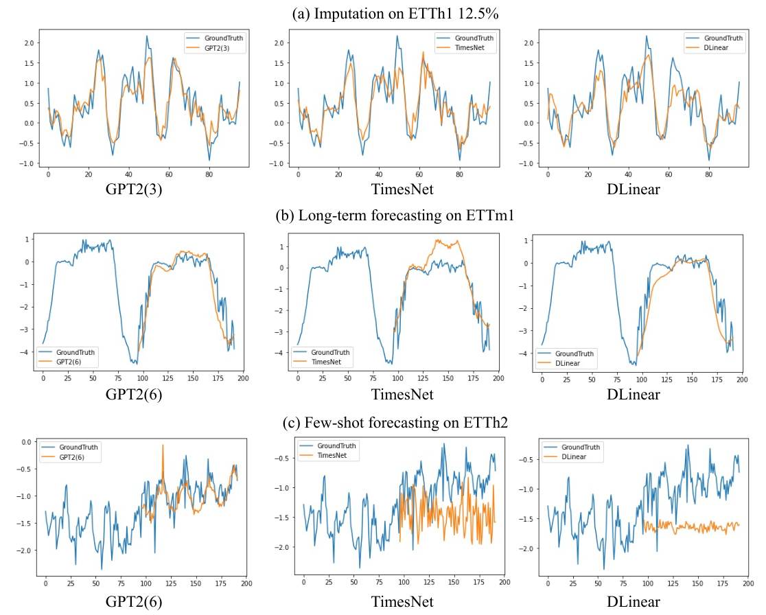
In order to clarify the representation ability more clearly, Figure 5 provides showcases of imputation, long-term forecasting and few-shot forecasting. Especially for few-shot learning, GPT2(6) can accurately forecast, while TimesNet and DLinear fail in this task.

Appendix B Related Works

We have presented a novel general time series analysis model in this paper, and to the best of our knowledge, there has been limited work on similar comprehensive methods for time series analysis. The most closely related field is time series forecasting, where transformer models have gained widespread popularity. Therefore, our focus in this related work will primarily be on introducing the end-to-end time series forecasting method.

Time series forecasting models can be roughly divided into three categories, ranging from the classic ARIMA models to the most recent transformer models. The first generation of well-discussed models can be dated back to auto-regressive family, such as ARIMA Box & Jenkins 1968; Box & Pierce 1970 that follows the Markov process and recursively execute sequential forecasting. However, it is limited to stationary sequences while most time series is non-stationary. Additionally, with the bloom of deep neural networks, recurrent neural networks (RNNs), such as LSTM Hochreiter & Schmidhuber 1997 and GRU Chung et al. 2014, were designed for sequential tasks. Yet the recurrent model is inefficient for training and long-term dependencies are still under resolved.

Recently, transformer models have achieve great progress in NLP Vaswani et al. 2017; Devlin et al. 2019; Radford et al. 2019 and CV Dosovitskiy et al. 2021; Bao et al. 2022 tasks. Also, a large amount of transformer models are proposed to apply to time series forecasting Wen et al. 2023. In the following, we briefly introduce several representative algorithms. Informer Zhou et al. 2021 proposes a probability sparse attention mechanism to deal with long-term dependencies. Autoformer Wu et al. 2021 introduces a decomposition transformer architecture and replaces the attention module with an Auto-Correlation mechanism. FEDformer Zhou et al. 2022 uses Fourier enhanced structure to improve computational efficiency and achieves linear complexity. Similar to patching in ViT Dosovitskiy et al. 2021, PatchTST Nie et al. 2022 employs segmentation of time series that divide a sequence into patches to increase input length and reduce information redundancy. Besides, a simple MLP-based model DLinear Zeng et al. 2023 outperforms most transformer models and it validates channel-independence works well in time series forecasting. Recently, TimesNet Wu et al. 2023 has treated time series as a 2D signal and utilized a convolution-based inception net backbone to function as a comprehensive time series analysis model. This work is closely related to our tasks in this paper.

Appendix C Dataset Details

In this section, we separately summarize dataset details long/short-term forecasting and few-shot/zero-shot forecasting.

Datasets of Long-term Forecasting and Few-shot Learning

The details of datasets are shown as follows: 1) ETT datasets Zhou et al. 2021 contain electricity load of various resolutions (ETTh & ETTm) from two electricity stations. 2) Weather contains 21 meteorological indicators of Germany within 1 year; 3) Illness contains the influenza-like illness patients in the United States; 4) Electricity dataset contains the electricity consumption; 5) Traffic dataset contains the occupation rate of freeway system across the State of California. Table 10 summarizes details of feature statistics.

Similar to PatchTST Nie et al. 2022, Exchange is not contained. Zeng et al. 2023 shows that simply repeating the last value in the look-back window can outperform or be comparable to the best results. Also, ILI is not used for few-shot learning for the limited quantity that is hard to follow the definition of few-shot.

Table 10: Dataset details of few-shot learning.

Dataset	Length	Dimension	Frequency
ETTh	17420	7	1 hour
ETTm	69680	7	15 min
Weather	52696	22	10 min
ILI	966	7	7 days
Electricity	26304	321	1 hour
Traffic	17544	862	1 hour

Datasets of Short-term Forecasting and Zero-shot Learning

The details of short-term forecasting and zero-shot learning datasets are shown as follows: 1) M4 is a large and diverse dataset that contains time series of various frequencies and fields, including business, financial and economic forecasting; 2) M3 is smaller than M4, but also contains time series from diverse domains and frequencies; 3) TOURISM is the dataset of tourism activities with different frequencies and contains a much higher fraction of erratic series compared with M4; 4) ELECTR represents the electricity usage monitoring of 370 customers over three years. Table 6 summarizes details of the datasets and zero-shot mapping between source and target.

Table 11: Datasets and mapping details of zero-shot learning.

	Dataset		Mapping
	Length	Horizon	M4	M3
M3 Yearly	645	6	Yearly	-
M3 Quarterly	756	8	Quarterly	-
M3 Monthly	1428	18	Monthly	-
M3 Others	174	8	Monthly	-
M4 Yearly	23000	6	-	Yearly
M4 Quarterly	24000	8	-	Quarterly
M4 Monthly	48000	18	-	Monthly
M4 Weekly	359	13	-	Monthly
M4 Daily	4227	14	-	Monthly
M4 Hourly	414	48	-	Monthly
TOURISM Yearly	518	4	Yearly	Yearly
TOURISM Quarterly	427	8	Quarterly	Quarterly
TOURISM Monthly	366	24	Monthly	Monthly
ELECTR	1311	168	Hourly	Monthly

Appendix D Experimental Details

All the deep learning networks are implemented in PyTorch and trained on NVIDIA V100 32GB GPUs. We use the pre-trained models from Wolf et al. 2020 for experiments. For few-shot learning, an early stopping counter is employed to stop the training process after three epochs if no loss degradation on the valid set is observed. Plus, we convert the multivariate data into univariate data. Specifically, we treat each feature of the sequence as a single time series. This is mainly for memory efficiency after patching of GPT2(6) and previous works, DLinear and PatchTST, have proved the effectiveness of channel-independence.

D.1 Accuracy Metrics

For long-term/short-term forecasting and few-shot forecasting, we use mean square error (MSE) and mean absolute error (MAE) as metrics. For zero-shot learning, mean absolute percentage error (MAPE) is used for TOURISM; symmetric MAPE (sMAPE) is used for M3 and M4; normalized deviation (ND) is used for ELECTR. All experiments are repeated 3 times and the mean of the metrics is used in the final results.

D.2 Detailed Definition and Results for Few-shot and Long-term Forecasting

Task Definition Since Zeng et al. 2023 and Nie et al. 2022 have verified that channel-independence works well for time series datasets, we treat each multivariate series as multiple independent univariate series. Similar to traditional experimental settings, each time series is split into three parts: training data, validation data, and test data. For the few-shot forecasting task, only a certain percentage ( $5\%$ , $10\%$ ) timesteps of training data are used, and the other two parts remain unchanged. The evaluation metrics remain the same as for classic multivariate time series forecasting. We repeat this experiment 3 times and report the average metrics in the following experiments.

Detail Experiment Tables for Few-shot Time-Series Forecasting in Table 12 and Table 13

Table 12: Few-shot learning results on 5% data. We use prediction length

O\in\{96,192,336,720\}

. A lower MSE indicates better performance, and the best results are highlighted in bold. ’-’ means that 5% time series is not sufficient to constitute a training set.

Methods		GPT2(6)		GPT2(0)		DLinear		PatchTST		TimesNet		FEDformer		Autoformer		Stationary		ETSformer		LightTS		Informer		Reformer
Metric		MSE	MAE	MSE	MAE	MSE	MAE	MSE	MAE	MSE	MAE	MSE	MAE	MSE	MAE	MSE	MAE	MSE	MAE	MSE	MAE	MSE	MAE	MSE	MAE
$Weather$	96	0.175	0.230	0.191	0.243	0.184	0.242	0.171	0.224	0.207	0.253	0.229	0.309	0.227	0.299	0.215	0.252	0.218	0.295	0.230	0.285	0.497	0.497	0.406	0.435
	192	0.227	0.276	0.244	0.289	0.228	0.283	0.230	0.277	0.272	0.307	0.265	0.317	0.278	0.333	0.290	0.307	0.294	0.331	0.274	0.323	0.620	0.545	0.446	0.450
	336	0.286	0.322	0.303	0.332	0.279	0.322	0.294	0.326	0.313	0.328	0.353	0.392	0.351	0.393	0.353	0.348	0.359	0.398	0.318	0.355	0.649	0.547	0.465	0.459
	720	0.366	0.379	0.391	0.393	0.364	0.388	0.384	0.387	0.400	0.385	0.391	0.394	0.387	0.389	0.452	0.407	0.461	0.461	0.401	0.418	0.570	0.522	0.471	0.468
	Avg.	0.263	0.301	0.282	0.314	0.263	0.308	0.269	0.303	0.298	0.318	0.309	0.353	0.310	0.353	0.327	0.328	0.333	0.371	0.305	0.345	0.584	0.527	0.447	0.453
$ETTh1$	96	0.543	0.506	0.825	0.638	0.547	0.503	0.557	0.519	0.892	0.625	0.593	0.529	0.681	0.570	0.952	0.650	1.169	0.832	1.483	0.91	1.225	0.812	1.198	0.795
	192	0.748	0.580	1.220	0.778	0.720	0.604	0.711	0.570	0.940	0.665	0.652	0.563	0.725	0.602	0.943	0.645	1.221	0.853	1.525	0.93	1.249	0.828	1.273	0.853
	336	0.754	0.595	1.852	0.965	0.984	0.727	0.816	0.619	0.945	0.653	0.731	0.594	0.761	0.624	0.935	0.644	1.179	0.832	1.347	0.87	1.202	0.811	1.254	0.857
	720	-	-	-	-	-	-	-	-	-	-	-	-	-	-	-	-	-	-	-	-	-	-	-	-
	Avg.	0.681	0.560	1.299	0.793	0.750	0.611	0.694	0.569	0.925	0.647	0.658	0.562	0.722	0.598	0.943	0.646	1.189	0.839	1.451	0.903	1.225	0.817	1.241	0.835
$ETTh2$	96	0.376	0.421	0.551	0.507	0.442	0.456	0.401	0.421	0.409	0.420	0.390	0.424	0.428	0.468	0.408	0.423	0.678	0.619	2.022	1.006	3.837	1.508	3.753	1.518
	192	0.418	0.441	0.765	0.610	0.617	0.542	0.452	0.455	0.483	0.464	0.457	0.465	0.496	0.504	0.497	0.468	0.845	0.697	3.534	1.348	3.975	1.933	3.516	1.473
	336	0.408	0.439	0.767	0.614	1.424	0.849	0.464	0.469	0.499	0.479	0.477	0.483	0.486	0.496	0.507	0.481	0.905	0.727	4.063	1.451	3.956	1.520	3.312	1.427
	720	-	-	-	-	-	-	-	-	-	-	-	-	-	-	-	-	-	-	-	-	-	-	-	-
	Avg.	0.400	0.433	0.694	0.577	0.827	0.615	0.439	0.448	0.463	0.454	0.441	0.457	0.47	0.489	0.470	0.457	0.809	0.681	3.206	1.268	3.922	1.653	3.527	1.472
$ETTm1$	96	0.386	0.405	0.582	0.512	0.332	0.374	0.399	0.414	0.606	0.518	0.628	0.544	0.726	0.578	0.823	0.587	1.031	0.747	1.048	0.733	1.130	0.775	1.234	0.798
	192	0.440	0.438	0.632	0.536	0.358	0.390	0.441	0.436	0.681	0.539	0.666	0.566	0.750	0.591	0.844	0.591	1.087	0.766	1.097	0.756	1.150	0.788	1.287	0.839
	336	0.485	0.459	0.767	0.584	0.402	0.416	0.499	0.467	0.786	0.597	0.807	0.628	0.851	0.659	0.870	0.603	1.138	0.787	1.147	0.775	1.198	0.809	1.288	0.842
	720	0.577	0.499	1.334	0.742	0.511	0.489	0.767	0.587	0.796	0.593	0.822	0.633	0.857	0.655	0.893	0.611	1.245	0.831	1.200	0.799	1.175	0.794	1.247	0.828
	Avg.	0.472	0.450	0.828	0.593	0.400	0.417	0.526	0.476	0.717	0.561	0.730	0.592	0.796	0.620	0.857	0.598	1.125	0.782	1.123	0.765	1.163	0.791	1.264	0.826
$ETTm2$	96	0.199	0.280	0.282	0.347	0.236	0.326	0.206	0.288	0.220	0.299	0.229	0.320	0.232	0.322	0.238	0.316	0.404	0.485	1.108	0.772	3.599	1.478	3.883	1.545
	192	0.256	0.316	0.346	0.383	0.306	0.373	0.264	0.324	0.311	0.361	0.394	0.361	0.291	0.357	0.298	0.349	0.479	0.521	1.317	0.850	3.578	1.475	3.553	1.484
	336	0.318	0.353	0.429	0.427	0.380	0.423	0.334	0.367	0.338	0.366	0.378	0.427	0.478	0.517	0.353	0.380	0.552	0.555	1.415	0.879	3.561	1.473	3.446	1.460
	720	0.460	0.436	0.751	0.568	0.674	0.583	0.454	0.432	0.509	0.465	0.523	0.510	0.553	0.538	0.475	0.445	0.701	0.627	1.822	0.984	3.896	1.533	3.445	1.460
	Avg.	0.308	0.346	0.452	0.431	0.399	0.426	0.314	0.352	0.344	0.372	0.381	0.404	0.388	0.433	0.341	0.372	0.534	0.547	1.415	0.871	3.658	1.489	3.581	1.487
$ECL$	96	0.143	0.241	0.147	0.246	0.150	0.251	0.145	0.244	0.315	0.389	0.235	0.322	0.297	0.367	0.484	0.518	0.697	0.638	0.639	0.609	1.265	0.919	1.414	0.855
	192	0.159	0.255	0.163	0.260	0.163	0.263	0.163	0.260	0.318	0.396	0.247	0.341	0.308	0.375	0.501	0.531	0.718	0.648	0.772	0.678	1.298	0.939	1.240	0.919
	336	0.179	0.274	0.182	0.278	0.175	0.278	0.183	0.281	0.340	0.415	0.267	0.356	0.354	0.411	0.574	0.578	0.758	0.667	0.901	0.745	1.302	0.942	1.253	0.921
	720	0.233	0.323	0.239	0.329	0.219	0.311	0.233	0.323	0.635	0.613	0.318	0.394	0.426	0.466	0.952	0.786	1.028	0.788	1.200	0.871	1.259	0.919	1.249	0.921
	Avg.	0.178	0.273	0.182	0.278	0.176	0.275	0.181	0.277	0.402	0.453	0.266	0.353	0.346	0.404	0.627	0.603	0.800	0.685	0.878	0.725	1.281	0.929	1.289	0.904
$Traffic$	96	0.419	0.298	0.468	0.354	0.427	0.304	0.404	0.286	0.854	0.492	0.670	0.421	0.795	0.481	1.468	0.821	1.643	0.855	1.157	0.636	1.557	0.821	1.586	0.841
	192	0.434	0.305	0.479	0.352	0.447	0.315	0.412	0.294	0.894	0.517	0.653	0.405	0.837	0.503	1.509	0.838	1.856	0.928	1.688	0.848	1.596	0.834	1.602	0.844
	336	0.449	0.313	0.477	0.345	0.478	0.333	0.439	0.310	0.853	0.471	0.707	0.445	0.867	0.523	1.602	0.860	2.080	0.999	1.826	0.903	1.621	0.841	1.668	0.868
	720	-	-	-	-	-	-	-	-	-	-	-	-	-	-	-	-	-	-	-	-	-	-	-	-
	Avg.	0.434	0.305	0.474	0.350	0.450	0.317	0.418	0.296	0.867	0.493	0.676	0.423	0.833	0.502	1.526	0.839	1.859	0.927	1.557	0.795	1.591	0.832	1.618	0.851
Average		0.377	0.375	0.575	0.465	0.441	0.413	0.392	0.383	0.552	0.464	0.483	0.445	0.537	0.480	0.697	0.537	0.909	0.675	1.341	0.789	1.878	0.994	1.819	0.966

Table 13: Few-shot learning results on 10% data. We use prediction length

O\in\{96,192,336,720\}

. A lower MSE indicates better performance, and the best results are highlighted in bold. ’-’ means that 10% time series is not sufficient to constitute a training set.

Methods		GPT2(6)		GPT2(0)		DLinear		PatchTST		TimesNet		FEDformer		Autoformer		Stationary		ETSformer		LightTS		Informer		Reformer
Metric		MSE	MAE	MSE	MAE	MSE	MAE	MSE	MAE	MSE	MAE	MSE	MAE	MSE	MAE	MSE	MAE	MSE	MAE	MSE	MAE	MSE	MAE	MSE	MAE
$Weather$	96	0.163	0.215	0.190	0.240	0.171	0.224	0.165	0.215	0.184	0.230	0.188	0.253	0.221	0.297	0.192	0.234	0.199	0.272	0.217	0.269	0.374	0.401	0.335	0.380
	192	0.210	0.254	0.243	0.284	0.215	0.263	0.210	0.257	0.245	0.283	0.250	0.304	0.270	0.322	0.269	0.295	0.279	0.332	0.259	0.304	0.552	0.478	0.522	0.462
	336	0.256	0.292	0.270	0.305	0.258	0.299	0.259	0.297	0.305	0.321	0.312	0.346	0.320	0.351	0.370	0.357	0.356	0.386	0.303	0.334	0.724	0.541	0.715	0.535
	720	0.321	0.339	0.348	0.359	0.320	0.346	0.332	0.346	0.381	0.371	0.387	0.393	0.390	0.396	0.441	0.405	0.437	0.448	0.377	0.382	0.739	0.558	0.611	0.500
	Avg.	0.238	0.275	0.263	0.297	0.241	0.283	0.242	0.279	0.279	0.301	0.284	0.324	0.300	0.342	0.318	0.323	0.318	0.360	0.289	0.322	0.597	0.495	0.546	0.469
$ETTh1$	96	0.458	0.456	0.601	0.536	0.492	0.495	0.516	0.485	0.861	0.628	0.512	0.499	0.613	0.552	0.918	0.639	1.112	0.806	1.298	0.838	1.179	0.792	1.184	0.790
	192	0.570	0.516	0.709	0.587	0.565	0.538	0.598	0.524	0.797	0.593	0.624	0.555	0.722	0.598	0.915	0.629	1.155	0.823	1.322	0.854	1.199	0.806	1.295	0.850
	336	0.608	0.535	0.801	0.635	0.721	0.622	0.657	0.550	0.941	0.648	0.691	0.574	0.750	0.619	0.939	0.644	1.179	0.832	1.347	0.870	1.202	0.811	1.294	0.854
	720	0.725	0.591	1.385	0.831	0.986	0.743	0.762	0.610	0.877	0.641	0.728	0.614	0.721	0.616	0.887	0.645	1.273	0.874	1.534	0.947	1.217	0.825	1.223	0.838
	Avg.	0.590	0.525	0.874	0.647	0.691	0.600	0.633	0.542	0.869	0.628	0.639	0.561	0.702	0.596	0.915	0.639	1.180	0.834	1.375	0.877	1.199	0.809	1.249	0.833
$ETTh2$	96	0.331	0.374	0.539	0.495	0.357	0.411	0.353	0.389	0.378	0.409	0.382	0.416	0.413	0.451	0.389	0.411	0.678	0.619	2.022	1.006	3.837	1.508	3.788	1.533
	192	0.402	0.411	0.675	0.555	0.569	0.519	0.403	0.414	0.490	0.467	0.478	0.474	0.474	0.477	0.473	0.455	0.785	0.666	2.329	1.104	3.856	1.513	3.552	1.483
	336	0.406	0.433	0.718	0.580	0.671	0.572	0.426	0.441	0.537	0.494	0.504	0.501	0.547	0.543	0.507	0.480	0.839	0.694	2.453	1.122	3.952	1.526	3.395	1.526
	720	0.449	0.464	0.732	0.605	0.824	0.648	0.477	0.480	0.510	0.491	0.499	0.509	0.516	0.523	0.477	0.472	1.273	0.874	3.816	1.407	3.842	1.503	3.205	1.401
	Avg.	0.397	0.421	0.666	0.559	0.605	0.538	0.415	0.431	0.479	0.465	0.466	0.475	0.488	0.499	0.462	0.455	0.894	0.713	2.655	1.160	3.872	1.513	3.485	1.486
$ETTm1$	96	0.390	0.404	0.610	0.508	0.352	0.392	0.410	0.419	0.583	0.501	0.578	0.518	0.774	0.614	0.761	0.568	0.911	0.688	0.921	0.682	1.162	0.785	1.442	0.847
	192	0.429	0.423	0.666	0.540	0.382	0.412	0.437	0.434	0.630	0.528	0.617	0.546	0.754	0.592	0.781	0.574	0.955	0.703	0.957	0.701	1.172	0.793	1.444	0.862
	336	0.469	0.439	0.895	0.615	0.419	0.434	0.476	0.454	0.725	0.568	0.998	0.775	0.869	0.677	0.803	0.587	0.991	0.719	0.998	0.716	1.227	0.908	1.450	0.866
	720	0.569	0.498	0.916	0.646	0.490	0.477	0.681	0.556	0.769	0.549	0.693	0.579	0.810	0.630	0.844	0.581	1.062	0.747	1.007	0.719	1.207	0.797	1.366	0.850
	Avg.	0.464	0.441	0.772	0.577	0.411	0.429	0.501	0.466	0.677	0.537	0.722	0.605	0.802	0.628	0.797	0.578	0.980	0.714	0.971	0.705	1.192	0.821	1.426	0.856
$ETTm2$	96	0.188	0.269	0.283	0.344	0.213	0.303	0.191	0.274	0.212	0.285	0.291	0.399	0.352	0.454	0.229	0.308	0.331	0.430	0.813	0.688	3.203	1.407	4.195	1.628
	192	0.251	0.309	0.353	0.384	0.278	0.345	0.252	0.317	0.270	0.323	0.307	0.379	0.694	0.691	0.291	0.343	0.400	0.464	1.008	0.768	3.112	1.387	4.042	1.601
	336	0.307	0.346	0.420	0.422	0.338	0.385	0.306	0.353	0.323	0.353	0.543	0.559	2.408	1.407	0.348	0.376	0.469	0.498	1.031	0.775	3.255	1.421	3.963	1.585
	720	0.426	0.417	0.553	0.491	0.436	0.440	0.433	0.427	0.474	0.449	0.712	0.614	1.913	1.166	0.461	0.438	0.589	0.557	1.096	0.791	3.909	1.543	3.711	1.532
	Avg.	0.293	0.335	0.402	0.410	0.316	0.368	0.296	0.343	0.320	0.353	0.463	0.488	1.342	0.930	0.332	0.366	0.447	0.487	0.987	0.756	3.370	1.440	3.978	1.587
$ECL$	96	0.139	0.237	0.142	0.240	0.150	0.253	0.140	0.238	0.299	0.373	0.231	0.323	0.261	0.348	0.420	0.466	0.599	0.587	0.350	0.425	1.259	0.919	0.993	0.784
	192	0.156	0.252	0.158	0.254	0.164	0.264	0.160	0.255	0.305	0.379	0.261	0.356	0.338	0.406	0.411	0.459	0.620	0.598	0.376	0.448	1.160	0.873	0.938	0.753
	336	0.175	0.270	0.175	0.271	0.181	0.282	0.180	0.276	0.319	0.391	0.360	0.445	0.410	0.474	0.434	0.473	0.662	0.619	0.428	0.485	1.157	0.872	0.925	0.745
	720	0.233	0.317	0.230	0.315	0.223	0.321	0.241	0.323	0.369	0.426	0.530	0.585	0.715	0.685	0.510	0.521	0.757	0.664	0.611	0.597	1.203	0.898	1.004	0.790
	Avg.	0.176	0.269	0.176	0.270	0.180	0.280	0.180	0.273	0.323	0.392	0.346	0.427	0.431	0.478	0.444	0.480	0.660	0.617	0.441	0.489	1.195	0.891	0.965	0.768
$Traffic$	96	0.414	0.297	0.478	0.368	0.419	0.298	0.403	0.289	0.719	0.416	0.639	0.400	0.672	0.405	1.412	0.802	1.643	0.855	1.157	0.636	1.557	0.821	1.527	0.815
	192	0.426	0.301	0.481	0.363	0.434	0.305	0.415	0.296	0.748	0.428	0.637	0.416	0.727	0.424	1.419	0.806	1.641	0.854	1.207	0.661	1.454	0.765	1.538	0.817
	336	0.434	0.303	0.488	0.365	0.449	0.313	0.426	0.304	0.853	0.471	0.655	0.427	0.749	0.454	1.443	0.815	1.711	0.878	1.334	0.713	1.521	0.812	1.550	0.819
	720	0.487	0.337	0.537	0.386	0.484	0.336	0.474	0.331	1.485	0.825	0.722	0.456	0.847	0.499	1.539	0.837	2.660	1.157	1.292	0.726	1.605	0.846	1.588	0.833
	Avg.	0.440	0.310	0.496	0.371	0.447	0.313	0.430	0.305	0.951	0.535	0.663	0.425	0.749	0.446	1.453	0.815	1.914	0.936	1.248	0.684	1.534	0.811	1.551	0.821
Average		0.371	0.367	0.521	0.447	0.413	0.401	0.385	0.376	0.556	0.458	0.511	0.472	0.687	0.559	0.674	0.522	0.912	0.665	1.137	0.712	1.850	0.967	1.888	0.974

D.3 Long-term Time-series Forecasting

Here we investigate whether our architecture performs consistently well with more training data. Thus, we follow the classical experiment settings of Nie et al. 2022 and conduct experiments on full data. The results are shown in Table 14. Overall, GPT2(6) FPT achieves comparable performance to PatchTST, Dlinear and outperforms other baselines by a large margin. Compared with the second best transformer-based baseline method FEDformer, GPT2(6) FPT yields an overall 18.7% relatively MSE reduction. It verifies the effectiveness of NLP pretrained model in time series forecasting, not limited to the few-shot setting.

Detail Experiment Table for Long-term Time-Series Forecasting in table 14

Table 14: Full results on full data. We use prediction length

O\in\{96,192,336,720\}

for ILI and

O\in\{24,36,48,60\}

for others. A lower MSE indicates better performance. Black: best, Red: second best.

Methods		GPT2(6)		GPT2(0)		DLinear		PatchTST		TimesNet		FEDformer		Autoformer		Stationary		ETSformer		LightTS		Informer		Reformer
Metric		MSE	MAE	MSE	MAE	MSE	MAE	MSE	MAE	MSE	MAE	MSE	MAE	MSE	MAE	MSE	MAE	MSE	MAE	MSE	MAE	MSE	MAE	MSE	MAE
$Weather$	96	0.162	0.212	0.181	0.232	0.176	0.237	0.149	0.198	0.172	0.220	0.217	0.296	0.266	0.336	0.173	0.223	0.197	0.281	0.182	0.242	0.300	0.384	0.689	0.596
	192	0.204	0.248	0.222	0.266	0.220	0.282	0.194	0.241	0.219	0.261	0.276	0.336	0.307	0.367	0.245	0.285	0.237	0.312	0.227	0.287	0.598	0.544	0.752	0.638
	336	0.254	0.286	0.270	0.299	0.265	0.319	0.245	0.282	0.280	0.306	0.339	0.380	0.359	0.395	0.321	0.338	0.298	0.353	0.282	0.334	0.578	0.523	0.639	0.596
	720	0.326	0.337	0.338	0.345	0.333	0.362	0.314	0.334	0.365	0.359	0.403	0.428	0.419	0.428	0.414	0.410	0.352	0.288	0.352	0.386	1.059	0.741	1.130	0.792
	Avg	0.237	0.270	0.252	0.285	0.248	0.300	0.225	0.264	0.259	0.287	0.309	0.360	0.338	0.382	0.288	0.314	0.271	0.334	0.261	0.312	0.634	0.548	0.803	0.656
$ETTh1$	96	0.376	0.397	0.422	0.428	0.375	0.399	0.370	0.399	0.384	0.402	0.376	0.419	0.449	0.459	0.513	0.491	0.494	0.479	0.424	0.432	0.865	0.713	0.837	0.728
	192	0.416	0.418	0.466	0.450	0.405	0.416	0.413	0.421	0.436	0.429	0.420	0.448	0.500	0.482	0.534	0.504	0.538	0.504	0.475	0.462	1.008	0.792	0.923	0.766
	336	0.442	0.433	0.488	0.464	0.439	0.443	0.422	0.436	0.491	0.469	0.459	0.465	0.521	0.496	0.588	0.535	0.574	0.521	0.518	0.488	1.107	0.809	1.097	0.835
	720	0.477	0.456	0.485	0.478	0.472	0.490	0.447	0.466	0.521	0.500	0.506	0.507	0.514	0.512	0.643	0.616	0.562	0.535	0.547	0.533	1.181	0.865	1.257	0.889
	Avg	0.427	0.426	0.465	0.455	0.422	0.437	0.413	0.430	0.458	0.450	0.440	0.460	0.496	0.487	0.570	0.537	0.542	0.510	0.491	0.479	1.040	0.795	1.029	0.805
$ETTh2$	96	0.285	0.342	0.318	0.368	0.289	0.353	0.274	0.336	0.340	0.374	0.358	0.397	0.346	0.388	0.476	0.458	0.340	0.391	0.397	0.437	3.755	1.525	2.626	1.317
	192	0.354	0.389	0.383	0.407	0.383	0.418	0.339	0.379	0.402	0.414	0.429	0.439	0.456	0.452	0.512	0.493	0.430	0.439	0.520	0.504	5.602	1.931	11.12	2.979
	336	0.373	0.407	0.406	0.427	0.448	0.465	0.329	0.380	0.452	0.452	0.496	0.487	0.482	0.486	0.552	0.551	0.485	0.479	0.626	0.559	4.721	1.835	9.323	2.769
	720	0.406	0.441	0.420	0.446	0.605	0.551	0.379	0.422	0.462	0.468	0.463	0.474	0.515	0.511	0.562	0.560	0.500	0.497	0.863	0.672	3.647	1.625	3.874	1.697
	Avg	0.354	0.394	0.381	0.412	0.431	0.446	0.330	0.379	0.414	0.427	0.437	0.449	0.450	0.459	0.526	0.516	0.439	0.452	0.602	0.543	4.431	1.729	6.736	2.191
$ETTm1$	96	0.292	0.346	0.330	0.372	0.299	0.343	0.290	0.342	0.338	0.375	0.379	0.419	0.505	0.475	0.386	0.398	0.375	0.398	0.374	0.400	0.672	0.571	0.538	0.528
	192	0.332	0.372	0.371	0.394	0.335	0.365	0.332	0.369	0.374	0.387	0.426	0.441	0.553	0.496	0.459	0.444	0.408	0.410	0.400	0.407	0.795	0.669	0.658	0.592
	336	0.366	0.394	0.398	0.409	0.369	0.386	0.366	0.392	0.410	0.411	0.445	0.459	0.621	0.537	0.495	0.464	0.435	0.428	0.438	0.438	1.212	0.871	0.898	0.721
	720	0.417	0.421	0.454	0.440	0.425	0.421	0.416	0.420	0.478	0.450	0.543	0.490	0.671	0.561	0.585	0.516	0.499	0.462	0.527	0.502	1.166	0.823	1.102	0.841
	Avg	0.352	0.383	0.388	0.403	0.357	0.378	0.351	0.380	0.400	0.406	0.448	0.452	0.588	0.517	0.481	0.456	0.429	0.425	0.435	0.437	0.961	0.734	0.799	0.671
$ETTm2$	96	0.173	0.262	0.192	0.281	0.167	0.269	0.165	0.255	0.187	0.267	0.203	0.287	0.255	0.339	0.192	0.274	0.189	0.280	0.209	0.308	0.365	0.453	0.658	0.619
	192	0.229	0.301	0.245	0.317	0.224	0.303	0.220	0.292	0.249	0.309	0.269	0.328	0.281	0.340	0.280	0.339	0.253	0.319	0.311	0.382	0.533	0.563	1.078	0.827
	336	0.286	0.341	0.302	0.352	0.281	0.342	0.274	0.329	0.321	0.351	0.325	0.366	0.339	0.372	0.334	0.361	0.314	0.357	0.442	0.466	1.363	0.887	1.549	0.972
	720	0.378	0.401	0.399	0.408	0.397	0.421	0.362	0.385	0.408	0.403	0.421	0.415	0.433	0.432	0.417	0.413	0.414	0.413	0.675	0.587	3.379	1.338	2.631	1.242
	Avg	0.266	0.326	0.284	0.339	0.267	0.333	0.255	0.315	0.291	0.333	0.305	0.349	0.327	0.371	0.306	0.347	0.293	0.342	0.409	0.436	1.410	0.810	1.479	0.915
$ILI$	24	2.063	0.881	2.723	1.099	2.215	1.081	1.319	0.754	2.317	0.934	3.228	1.260	3.483	1.287	2.294	0.945	2.527	1.020	8.313	2.144	5.764	1.677	4.400	1.382
	36	1.868	0.892	2.027	0.966	1.963	0.963	1.430	0.834	1.972	0.920	2.679	1.080	3.103	1.148	1.825	0.848	2.615	1.007	6.631	1.902	4.755	1.467	4.783	1.448
	48	1.790	0.884	2.206	1.022	2.130	1.024	1.553	0.815	2.238	0.940	2.622	1.078	2.669	1.085	2.010	0.900	2.359	0.972	7.299	1.982	4.763	1.469	4.832	1.465
	60	1.979	0.957	1.976	0.983	2.368	1.096	1.470	0.788	2.027	0.928	2.857	1.157	2.770	1.125	2.178	0.963	2.487	1.016	7.283	1.985	5.264	1.564	4.882	1.483
	Avg	1.925	0.903	2.233	1.017	2.169	1.041	1.443	0.797	2.139	0.931	2.847	1.144	3.006	1.161	2.077	0.914	2.497	1.004	7.382	2.003	5.137	1.544	4.724	1.445
$ECL$	96	0.139	0.238	0.138	0.234	0.140	0.237	0.129	0.222	0.168	0.272	0.193	0.308	0.201	0.317	0.169	0.273	0.187	0.304	0.207	0.307	0.274	0.368	0.312	0.402
	192	0.153	0.251	0.152	0.247	0.153	0.249	0.157	0.240	0.184	0.289	0.201	0.315	0.222	0.334	0.182	0.286	0.199	0.315	0.213	0.316	0.296	0.386	0.348	0.433
	336	0.169	0.266	0.168	0.263	0.169	0.267	0.163	0.259	0.198	0.300	0.214	0.329	0.231	0.338	0.200	0.304	0.212	0.329	0.230	0.333	0.300	0.394	0.350	0.433
	720	0.206	0.297	0.207	0.295	0.203	0.301	0.197	0.290	0.220	0.320	0.246	0.355	0.254	0.361	0.222	0.321	0.233	0.345	0.265	0.360	0.373	0.439	0.340	0.420
	Avg	0.167	0.263	0.166	0.259	0.166	0.263	0.161	0.252	0.192	0.295	0.214	0.327	0.227	0.338	0.193	0.296	0.208	0.323	0.229	0.329	0.311	0.397	0.338	0.422
$Traffic$	96	0.388	0.282	0.390	0.272	0.410	0.282	0.360	0.249	0.593	0.321	0.587	0.366	0.613	0.388	0.612	0.338	0.607	0.392	0.615	0.391	0.719	0.391	0.732	0.423
	192	0.407	0.290	0.403	0.276	0.423	0.287	0.379	0.256	0.617	0.336	0.604	0.373	0.616	0.382	0.613	0.340	0.621	0.399	0.601	0.382	0.696	0.379	0.733	0.420
	336	0.412	0.294	0.413	0.280	0.436	0.296	0.392	0.264	0.629	0.336	0.621	0.383	0.622	0.337	0.618	0.328	0.622	0.396	0.613	0.386	0.777	0.420	0.742	0.420
	720	0.450	0.312	0.447	0.298	0.466	0.315	0.432	0.286	0.640	0.350	0.626	0.382	0.660	0.408	0.653	0.355	0.632	0.396	0.658	0.407	0.864	0.472	0.755	0.423
	Avg	0.414	0.294	0.413	0.281	0.433	0.295	0.390	0.263	0.620	0.336	0.610	0.376	0.628	0.379	0.624	0.340	0.621	0.396	0.622	0.392	0.764	0.416	0.741	0.422
Average		0.516	0.407	0.573	0.0.431	0.562	0.436	0.446	0.386	0.596	0.433	0.701	0.489	0.757	0.511	0.633	0.465	0.662	0.473	1.303	0.616	1.836	0.871	2.081	0.954

D.4 Mean and STD for Few-shot Learning

Table 15 lists both mean and STD for GPT2(6), DLinear and PatchTST with 3 runs on 5% ETTh2 and ETTm2. The results show a small variance in performance of GPT2(6) that represents the stability of GPT2(6).

Table 15: A subset of results showing both Mean and STD on 5% datasets.

Methods		GPT2-backbone(6 Layers)
Metric		MSE	MAE
$ETTh2$	96	0.376 $\pm$ 0.0072	0.421 $\pm$ 0.0054
	192	0.418 $\pm$ 0.0013	0.441 $\pm$ 0.0014
	336	0.408 $\pm$ 0.0006	0.439 $\pm$ 0.0002
	720	-	-
$ETTm2$	96	0.199 $\pm$ 0.0040	0.280 $\pm$ 0.0042
	192	0.256 $\pm$ 0.0030	0.316 $\pm$ 0.0017
	336	0.318 $\pm$ 0.0046	0.353 $\pm$ 0.0032
	720	0.460 $\pm$ 0.0132	0.436 $\pm$ 0.0066

D.5 Comparison with Traditional Methods on Few-shot Learning

Since deep learning methods are more advantageous than traditional methods when applied to large datasets. For few-shot learning, traditional methods should also consider. The results are shown in Table 16 that GPT2(6) also achieves best performance.

Table 16: Comparison with traditional methods.

Methods		GPT2(6) 5%		GPT2(6) 10%		ETS		ARIMA		NaiveDrift
Metric		MSE	MAE	MSE	MAE	MSE	MAE	MSE	MAE	MSE	MAE
$ETTh2$	96	0.376	0.421	0.331	0.374	2.954	0.742	0.481	0.443	0.764	0.561
$ETTh2$	192	0.418	0.441	0.402	0.411	10.226	1.212	0.585	0.495	1.560	0.785
$ETTm1$	96	0.386	0.405	0.390	0.404	52.237	2.689	0.693	0.547	1.539	0.913
$ETTm1$	192	0.440	0.438	0.429	0.423	186.445	4.654	0.710	0.557	2.869	1.215

D.6 Baselines with Instance Normalization

Instance normalization Kim et al. 2022 is a plug-in for time series for distribution shift. Most baselines, such as Autoformer and FEDformer are not equipped with instance normalization. Thus, for a fair comparison, we add the experiment, as in Table 17, for baselines w/o instance normalization and GPT(6) can also perform superior.

Table 17: Comparison on 5% data. Autoformer and FEDformer are equiped with instance normalization.

Methods		GPT2(6)		PatchTST		DLinear		Autoformer		Autoformer(Revin)		FEDformer		FEDformer(Revin)
Metric		MSE	MAE	MSE	MAE	MSE	MAE	MSE	MAE	MSE	MAE	MSE	MAE	MSE	MAE
$ETTm2$	96	0.199	0.280	0.206	0.288	0.236	0.326	0.232	0.322	0.224	0.300	0.229	0.320	0.223	0.298
$ETTm2$	192	0.256	0.316	0.264	0.324	0.306	0.373	0.291	0.357	0.296	0.343	0.294	0.361	0.288	0.336

D.7 Detailed Definition and Results of Zero-shot Learning

Task Definition Each experiment contains two distinct datasets, source, and target datasets. The source dataset is used to train the model and then forecasts without fine-tuning in the target dataset. The target dataset is split into non-overlapping historical and test sequences. We use the historical sequence as input to the model, and the obtained output is used to calculate errors with the test sequences. Besides meta-learning-based models like N-BEATS, evaluated models’ parameters are not allowed any adjustment using the forecasting phase. Also, same as Oreshkin et al. 2021, each data set adopts a specific metric (M4: sMAPE; M3: sMAPE; TOURISM: MAPE; ELECTR: ND)

Detailed Results Here, we list detailed performance of zero-shot learning in Table 18, Table 19 and Table 20. For each dataset, we separately list the performance of models under diverse frequency. Compared to the most recent published method DLinear, GPT2(6) performs superior in most situations. Also, GPT2(6) does not use any information from the test data, but achieves a comparable performance of meta-leaning based N-BEATS.

Table 18: Zero-shot performance on M4 (sMAPE).

	Yearly	Quarterly	Monthly	Others	Average
	(23k)	(24k)	(48k)	(5k)	(100k)
N-BEATS-FR	13.267	9.596	12.676	4.696	11.675
DLinear-M3	14.193	18.856	14.765	9.194	15.337
TimesNet-M3	15.655	11.877	16.165	6.863	14.553
PatchTST-M3	13.966	10.929	14.664	7.087	13.228
ETSformer-M3	27.846	36.134	25.114	12.338	27.748
LightTS-M3	13.787	11.289	15.181	9.117	13.623
Stationary-M3	14.988	11.686	16.098	6.977	14.327
FEDformer-M3	13.887	11.513	18.154	7.529	15.047
Autoformer-M3	14.552	17.341	25.063	9.666	20.022
Informer-M3	18.542	16.907	23.454	7.348	19.047
Reformer-M3	15.652	11.051	15.604	7.001	14.092
GPT(6)-M3	13.740	10.787	14.630	7.081	13.125

Table 19: Zero-shot performance on M3 (sMAPE).

	Yearly	Quarterly	Monthly	Others	Average
	(645)	(756)	(1428)	(174)	(3003)
N-BEATS-M4	15.07	9.07	13.19	4.29	12.38
N-BEATS-FR	16.43	9.05	13.30	4.51	12.61
DLinear-M4	17.43	9.74	15.65	6.81	14.03
TimesNet-M4	18.75	12.26	14.01	6.88	14.17
PatchTST-M4	15.99	9.62	14.71	9.44	13.39
ETSformer-M4	20.56	11.65	16.97	10.57	16.03
LightTS-M4	15.63	9.40	24.60	8.28	17.90
Stationary-M4	17.05	12.56	16.82	8.13	15.29
FEDformer-M4	16.00	9.48	15.12	8.94	13.53
Autoformer-M4	16.18	13.92	16.91	14.68	15.87
Informer-M4	19.70	13.00	15.91	13.03	15.82
Reformer-M4	16.03	9.76	14.80	7.53	13.37
GPT2(6)-M4	16.42	10.13	14.10	4.81	13.06

Table 20: Zero-shot performance on Tourism (MAPE).

	Yearly	Quarterly	Monthly	Average
	(518)	(427)	(366)	(1311)
N-BEATS-M4	23.57	14.66	19.32	18.82
N-BEATS-FR	23.43	14.45	20.47	19.46
DLinear-M4	39.59	18.30	24.76	28.51
TimesNet-M4	35.59	19.22	30.54	28.84
PatchTST-M4	33.23	19.27	27.57	27.10
ETSformer-M4	391.60	35.56	50.47	180.40
LightTS-M4	138.22	16.28	25.34	66.99
Stationary-M4	35.42	35.15	65.58	43.75
FEDformer-M4	43.41	19.88	28.39	31.55
Autoformer-M4	51.19	34.95	31.47	40.39
Informer-M4	41.16	30.98	33.92	35.82
Reformer-M4	33.86	16.85	23.71	25.48
GPT2(6)-M4	27.17	16.21	21.92	22.14

Appendix E Proof

In our numerical experiments, we obtain two interesting observations. First, the token similarity within a sample is larger in pretrained LM. We report the layer-wise average token cosine similarity in ETTh2 experiment in Figure 7. In particular, Figure 7 (a) shows that in a fine-tuned random initialed GPT2(6) model, the token similarity is around 0.1-0.2 among different layers. When switching to the frozen pre-trained GPT2-FPT model, the token similarity significantly increases in the deep layers and eventually reaches more than 0.9 in the last layer. The ETTh2 dataset contains high volatility hourly information related to the electricity transformer temperature. In this situation, higher token similarity implies the high-frequency noise in the data is eased and only low-frequency information will be reserved. In other words, after going through the pretrained GPT2-FPT model, the signal-noise ratio is enhanced. We use the following theorem to characterize this behavior.

E.1 Theorem E.1

Theorem E.1 (informal).

We consider the self-attention for $l$ -th query token. Let’s assume the input token $\bm{x}_{i}$ are bounded with mean $\bm{\mu}$ for $i=1,2,...,n$ . Under mild conditions, with high probability, the output value token $\bm{V}_{l}$ converges to $\bm{\mu}W_{v}$ on the order of $\mathcal{O}(n^{-1/2})$ , where $W_{v}$ is the parameter matrix to compute the value token.

The Theorem E.1 describes the self-attention structure can efficiently make output value token $\bm{V}_{l}$ converge its mean value $\bm{\mu}W_{v}$ . In the time series forecasting task, each token represents several adjacent points in a time series. When the time series has some periodical or translation invariant structures, by comparing a given token with other tokens, one could have a higher chance to figure out those invariant structures. This phenomenon is especially important in few-shot forecasting tasks. Without enough token noise distillation ability, the model will more likely tend to overfit due to insufficient training data.

We denote $x_{i}$ as $i$ -th element of vector $\bm{x}$ , $\bm{W}_{ij}$ as the element at $i$ -th row and $j$ -th column of matrix $\bm{W}$ , and $\bm{W}_{j}$ as the $j$ -th row of matrix $\bm{W}$ . Moreover, we denote $\bm{x}_{i}$ as the $i$ -th patch (token) of the inputs with $\bm{x}_{i}=\bm{X}_{i}$ .

Before given the formal statement of the Theorem E.1, we first show the assumptions.

1.

The token $\bm{x}_{i}$ is the sub-gaussian random vector with mean $\bm{\mu}_{i}$ and variance $(\sigma^{2}/d)I$ for $i=1,2,...,n$ .
2.

$\bm{\mu}$ follows a discrete distribution with finite values $\bm{\mu}\in\mathcal{V}$ . Moreover, there exist $0<\nu_{1},0<\nu_{2}<\nu_{4}$ such that a) $\|\bm{\mu}_{i}\|=\nu_{1}$ , and b) $\bm{\mu}_{i}\bm{W}_{\bm{Q}}\bm{W}_{\bm{K}}^{T}\bm{\mu}_{i}\in[\nu_{2},\nu_{4}]$ for all $i$ and $|\bm{\mu}_{i}\bm{W}_{\bm{Q}}\bm{W}_{\bm{K}}^{\top}\bm{\mu}_{j}^{\top}|\leq\nu_{2}$ for all $\bm{\mu}_{i}\neq\bm{\mu}_{j}\in\mathcal{V}$ .
3.

$\bm{W}_{V}$ and $\bm{W}_{\bm{Q}}\bm{W}_{\bm{K}}^{\top}$ are element-wise bounded with $\nu_{5}$ and $\nu_{6}$ respectively, that is, $|\bm{W}_{V}^{(ij)}|\leq\nu_{5}$ and $|(\bm{W}_{\bm{Q}}\bm{W}_{\bm{K}}^{\top})^{(ij)}|\leq\nu_{6}$ , for all $i,j$ from 1 to $d$ .

In the above assumptions, we ensure that for a given query patch, the difference between the clustering center and noises are large enough to be distinguished.

Theorem E.2 (formal statement of Theorem E.1).

Let patch $\bm{x}_{i}$ be $\sigma^{2}$ -subgaussian random variable with mean $\bm{\mu}_{i}$ and all $n$ patches follow the same clustering center of query $l$ . Per Assumptions aforementioned, when $\sqrt{d}\geq 3(\psi(\delta,d)+\nu_{2}+\nu_{4})$ , then with probability $1-5\delta$ , we have

		$\displaystyle\left\\|\frac{\sum_{i=1}^{n}\exp\left(\frac{1}{\sqrt{d}}\bm{x}_{l}\bm{W}_{\bm{Q}}\bm{W}^{\top}_{k}\bm{x}_{i}\right)\bm{x}_{i}\bm{W}_{V}}{\sum_{j=1}^{n}\exp\left(\frac{1}{\sqrt{d}}\bm{x}_{l}\bm{W}_{\bm{Q}}\bm{W}_{\bm{K}}^{\top}\bm{x}_{j}\right)}-\bm{\mu}_{l}\bm{W}_{V}\right\\|_{\infty}\leq 4\exp\left(\frac{\psi(\delta,d)}{\sqrt{d}}\right)\sigma\nu_{5}\sqrt{\frac{2}{dn}\log\left(\frac{2d}{\delta}\right)}$
		$\displaystyle+7\left[\exp\left(\frac{\nu_{2}-\nu_{4}+\psi(\delta,d)}{\sqrt{d}}\right)-1\right]\\|\bm{\mu}_{l}\bm{W}_{V}\\|_{\infty},$

where $\psi(\delta,d)=2\sigma\nu_{1}\nu_{6}\sqrt{2\log\left(\frac{1}{\delta}\right)}+2\sigma^{2}\nu_{6}\log\left(\frac{d}{\delta}\right)$ .

Proof.

See the proof of Lemma 2 in Wang et al. 2022 with $k_{1}=k=n$ . ∎

E.2 Theorem E.4

We first give the formal statement of Theorem E.4.

Theorem E.3 (formal statement of Theorem E.4).

Let $\bm{g}_{i}\in\mathbbm{R}^{d}$ and $\bm{y}_{i}\in\mathbbm{R}^{T}$ be the feature map vector and forecasting targets for the sample $i=1,2,...,N$ respectively, and we assume $\frac{1}{N}\sum_{i=1}^{N}\bm{g}_{i}\bm{g}_{i}^{\top}\succeq\sigma I$ for some $\sigma>0$ . We want to learn a matrix $\bm{W}\in\mathbbm{R}^{d\times T}$ from the following optimization problem:

\displaystyle\bm{W}=\arg\min\frac{1}{2N}\sum_{i=1}^{N}\|\bm{W}\bm{g}_{i}-\bm{y}_{i}\|_{2}^{2}.

(1)

If we apply stochastic gradient descent with diminishing step sizes $\eta_{t}=\frac{1}{\sigma t}$ at step $t$ , we will need $t=\tilde{\mathcal{O}}(\epsilon^{-1}\sigma^{-1})$ steps to reach

\displaystyle\frac{1}{t}\sum_{j=1}^{t}\left(\frac{1}{2N}\sum_{i=1}^{N}\|\bm{W}_{j}\bm{g}_{i}-\bm{y}_{i}\|_{2}^{2}\right)-\frac{1}{2N}\sum_{i=1}^{N}\|\bm{W}^{*}\bm{g}_{i}-\bm{y}_{i}\|_{2}^{2}\leq\epsilon,

(2)

where $\bm{W}^{*}$ is the optimal solution and $\bm{W}_{j}$ is the $j$ step’s solution and $\tilde{\mathcal{O}}$ we suppress the logarithmic dependence.

Proof.

As we assume $\frac{1}{N}\sum_{i=1}^{T}\bm{g_{i}}\bm{g}_{i}^{\top}\succeq\sigma I$ , the hessian of optimization problem in (1) is also positive definite, which is equivalent to the optimization problem in (1) is strongly convex with parameter proportional to $\sigma$ . Then via standard stochastic gradient decent analysis (e.g., section 3.1 in Lacoste-Julien et al. 2012), we obtain:

\displaystyle\frac{1}{t}\sum_{j=1}^{t}\left(\frac{1}{2N}\sum_{i=1}^{N}\|\bm{W}_{j}\bm{g}_{i}-\bm{y}_{i}\|_{2}^{2}\right)-\frac{1}{2N}\sum_{i=1}^{N}\|\bm{W}^{*}\bm{g}_{i}-\bm{y}_{i}\|_{2}^{2}\leq\mathcal{O}\left(\frac{\log t}{\sigma t}\right)=\tilde{O}(\sigma^{-1}t^{-1}).

(3)

Therefore, to reach $\epsilon$ optimization gap, we just need to set $t=\tilde{\mathcal{O}}(\sigma^{-1}\epsilon^{-1})$ . ∎

The second observation is that for the pretrained GPT2-FPT model, the last transformer layer’s outputs, i.e., feature maps, are spread widely throughout the feature space. We report the t-SNE visualization of the feature maps for GPT2-FPT and an end-to-end model PatchTST in Figure 8. In Figure 8 (a) and (b), we color the samples chunked from the one single time series into the same color and the same configuration of the T-SNE is applied. One may observe that the feature maps of GPT2-FPT has less concentration compared to PatchTST. It implies the GPT2-FPT’s feature maps corresponding to different samples are more distinctive which eventually facilitates the learning ability of the last MLP layer. Researchers Wang & Isola 2020 have found that contrastive learning-based representation learning may result in a uniform distribution of training data, and such behavior plays an important role in its good downstream task performance. We use the following theorem to justify it.

Theorem E.4 (informal).

Let $\bm{g}_{i}$ and $\bm{y}_{i}$ be the feature map vector and forecasting targets for the sample $i=1,2,...,N$ respectively, and we assume $\frac{1}{N}\sum_{i=1}^{N}\bm{g}_{i}\bm{g}_{i}^{\top}\succeq\sigma I$ for some $\sigma>0$ . Under mild conditions, if we train an MLP layer that maps feature maps to forecasting targets via the stochastic gradient descent, the total step to reach some optimization tolerance is on the order of $\mathcal{O}(\sigma^{-1})$ .

The Theorem E.4 considers the covariate matrix of feature maps being positive definite that indicates the set of all feature maps $\{\bm{g}_{i}\}$ spans the whole feature spaces, and the higher spread level gives a larger $\sigma$ . In this case, if we only want to learn an MLP layer, the problem reduces to a well-conditioned least-squared regression problem. Then the fast convergence rate is achieved.

Efficiently learning the last MLP layer plays a very important role in time series forecasting and can substantially impact the prediction performance. In Zeng et al. 2023, the authors show that learning a single MLP layer can also bring very promising performance. In few-shot forecasting, the pre-trained GPT2 model may still preserve highly diverse feature maps than end-to-end type models and eventually leads to fast learning speed on the last MLP layer.

Another possible benefit of wide spared feature maps is enhancing the model memorization ability when using a multi-layer decoder structure. In the literature on network memorization ability (e.g., Vardi et al. 2021; Yun et al. 2020), the deep learning model tends to have better memorization ability when feature maps are well separated. In forecasting tasks, capturing extreme or rare behavior is very important. The pretrained GPT gains more capacity in the decoder to correctly forecast uncommon time series.

Appendix F N-gram Explanation for Universality

Why does the proposed pretrained-frozen-model work so effectively? We have achieved state-of-the-art performance in time series analysis using a language model that is mostly trained on natural language data. The answer lies in the universality of the frozen structure, which includes attention layers and Feed Forward layers. We can represent images and time series forecasting tasks as an n-gram estimation problem, akin to text analysis, by employing a patching approach. This method treats subsequences of time series or image patches as individual tokens. Central to sequential prediction is the $n$ -order Markov process, and a simple way to capture the $n$ -order Markov process is $n$ -gram language model. To predict next token $w_{0}$ , we need to compute $p(w_{0}|w_{1},\ldots,w_{n-1})$ , which can be further computed as $p(w_{0}w_{1}\ldots w_{n-1})/p(w_{1}\ldots w_{n-1})$ . Hence, the core of $n$ -gram language model is to estimate the probability of observing a sequence of $n$ tokens. When $n$ is large, most of $n$ token sequences will not be observed from data, leading to the sparse data problem, a common challenge faced by $n$ -gram language model. As a result, a large body of research in $n$ -gram language model is focused on how to effectively estimate probability of having $n$ -token sequences even when they are NOT observed from data. We hypothesize that the transformer model pretrained by GPT-2 essentially allows us to estimate $p(w_{0}w_{1}\ldots w_{n-1})$ from observations of significantly shorter token sequences. In this section, we will show that the function of estimating probabilities of longer sequences from observation of shorter sequences is universal and is independent from domain as long as data exhibit a skew distribution (e.g., follows a power law). We note that our work is closely related to the discussion presented in Elhage et al. 2021; Olsson et al. 2022, where the authors also connect the function of transformer to compute of $n$ -grams. We however note that our key result is to show the universality in computing probability of longer sequences from observations of shorter sequences, which can’t be found in any existing studies. Although the discussion is restricted to discrete tokens, it should be generalized to continuous signals as we can always quantize continuous signals into a finite number of discrete tokens, similar to what BEiT Bao et al. 2022 did.

To gain a better understanding, let’s start by examining a "zero-layer" Transformer model. This model operates by taking a token, embedding it, and transforming it back to produce logits that predict the subsequent token. Because it cannot transfer information from other tokens, it relies solely on the current token to predict the next one. Consequently, the optimal behavior of this model is to closely resemble the bigram log-likelihood.

Then we move on to the so-called "attention-only" transformer, which doesn’t have MLP layers. As discussed in a recent work Elhage et al. 2021, one-layer attention-only Transformers can be comprehended as a combination of a bigram model and multiple "skip-trigram" models (impacting the probabilities of sequences "A… BC"). This can be intuitively understood as each attention head having the ability to selectively attend from the current token ("B") to a previous token ("A") and transfer relevant information to fine-tune the probability of potential subsequent tokens ("C"). Olsson et al. 2022 further discusses a multi-layer transformer can do more complex n-gram estimation using an induction heads mechanism. To be more precise, induction heads employ a straightforward principle: the ’[A][B] … [A] → [B]’ rule, which elevates the likelihood of generating the subsequent token ’B’ given the current token ’A’ if there is a fuzzy match of the AB bigram in the historical context. This rule seems to largely decouple A and B, which means they do not memorize a fixed table of n-gram statistics. The rule [A][B] … [A] → [B] applies regardless of what A and B are, which can abstract to new patterns.

Building upon these discussions, we are now prepared to substantiate the following argument: For sequential data following a power law, there is a potentially universal solution to the final estimation of n-gram probabilities. That’s the reason behind the universality of pretrained LM’s performance in cross-domain tasks. For simplicity, we assume that $n$ is so large that we are unable to observe any occurrence of $n$ -gram from data, and we only observe the occurrence of $n^{\prime}$ -grams with $n^{\prime}<n$ . We denote by $s^{n}_{i}$ the $i$ th unique $n$ -gram, and by the notation $s^{n^{\prime}}_{j}\in s^{n}_{i}$ if $n^{\prime}$ -gram $s^{n^{\prime}}_{j}$ appears in $s^{n}_{i}$ , the $i$ th $n$ -gram. Let $m_{n}$ be the number of unique $n$ -grams. According to the maximum entropy model, our estimation of n-gram probabilities can be cast into the following optimization problem:

$\begin{array}[]{rcl}\min\ \sum_{i=1}^{m_{n}}p(s^{n}_{i})\log p(s^{n}_{i})\quad\mbox{s. t.}\sum_{i:s^{n^{\prime}}_{j}\in s^{n}_{i}}p(s^{n}_{i})=\widehat{p}(s^{n^{\prime}}_{j})\end{array}$

where $\widehat{p}(s^{n^{\prime}}_{j})$ represents the probability of observing pattern $s^{n^{\prime}}_{j}$ from the data and $j\in[m_{n^{\prime}}],n^{\prime}\in[n-1]$ .

For each constraint for $\widehat{p}(s_{j}^{n^{\prime}})$ , we introduce a Lagrangian dual variable $\lambda_{j}^{n^{\prime}}$ , and rewrite the optimization problem as follows:

$\begin{array}[]{rcl}\min_{\lambda}\ \log\left(\sum_{i=1}^{m_{n}}\exp\left(\sum_{(n^{\prime},j):s^{n^{\prime}}_{j}\in s^{n}_{i}}\lambda_{j}^{n^{\prime}}\right)\right)-\sum_{n^{\prime}=1}^{n-1}\sum_{j=1}^{m_{n^{\prime}}}\lambda_{j}^{n^{\prime}}\widehat{p}(s^{n^{\prime}}_{j}),\end{array}$

where n-gram probability $p(s^{n}_{j})$ is given as $p(s^{n}_{j})=\frac{1}{Z(\lambda)}\exp\left(\sum_{(n^{\prime},j):s_{j}^{n^{\prime}}\in s_{i}^{n}}\lambda^{n^{\prime}}_{j}\right)$ and $Z(\lambda)=\sum_{i=1}^{m_{n}}\exp(\sum_{(n^{\prime},j):s_{j}^{n^{\prime}}\in s_{i}^{n}}\lambda^{n^{\prime}}_{j})$

In the case that all n-grams follow a power law, for each $n^{\prime}\in[n-1]$ , we divide $n^{\prime}$ -gram into two groups: the group $\mathcal{V}_{n^{\prime}}$ includes the high frequency $n^{\prime}$ -gram and the group $\mathcal{U}_{n^{\prime}}$ including the low frequency of $n^{\prime}$ -gram. For simplicity, we assume that the probability for all the high frequency $n^{\prime}$ -grams are roughly $\alpha_{n^{\prime}}\in[0,1]$ and the probability for all the low frequency $n^{\prime}$ -grams are roughly $\beta_{n^{\prime}}\in[0,1]$ . By assuming that all the patterns in $\mathcal{V}_{n^{\prime}}$ and $\mathcal{U}_{n^{\prime}}$ share similar appearance frequency, we simplify the optimization problem by only introducing two dual variables for each $n^{\prime}$ -gram, i.e. $\lambda_{a}^{n^{\prime}}$ for high-frequency patterns and $\lambda_{b}^{n^{\prime}}$ for low-frequency patterns as follow Using these notations, we have the optimization problem simplified as

$\begin{array}[]{rcl}\min_{\lambda}\quad\log(\sum_{i=1}^{m_{n}}\exp(\sum_{n^{\prime}=1}^{n-1}\sum_{j:s^{n^{\prime}}_{j}\in s^{n}_{i}}\lambda_{a}^{n^{\prime}}I(s_{j}^{n^{\prime}}\in\mathcal{V}_{n^{\prime}})\\ +\lambda_{b}^{n^{\prime}}I(s_{j}^{n^{\prime}}\in\mathcal{U}_{n^{\prime}})))-\sum_{n^{\prime}=1}^{n-1}\left(\lambda_{a}^{n^{\prime}}g_{n^{\prime}}+\lambda_{b}^{n^{\prime}}h_{n^{\prime}}\right),\end{array}$

where $g_{n^{\prime}}=\sum_{s^{n^{\prime}}_{j}\in\mathcal{V}_{n^{\prime}}}\widehat{p}(s^{n^{\prime}}_{j})$ and $\quad h_{n^{\prime}}=\sum_{s^{n^{\prime}}_{j}\in\mathcal{U}_{n^{\prime}}}\widehat{p}(s^{n^{\prime}}_{j})$ .

Furthermore, let $q^{n^{\prime}}_{a}$ be the probability to observe a high frequency $n^{\prime}$ -gram appearing in any $n$ -gram, and $q^{n^{\prime}}_{b}$ be the probability to observe a low frequency $n^{\prime}$ -gram appearing in any $n$ -gram, we have

$\begin{array}[]{rcl}&\sum_{i=1}^{m_{n}}\exp(\sum_{n^{\prime}=1}^{n-1}\sum_{j:s^{n^{\prime}}_{j}\in s^{n}_{i}}\lambda_{a}^{n^{\prime}}I(s_{j}^{n^{\prime}}\in\mathcal{V}_{n^{\prime}})+\lambda_{b}^{n^{\prime}}I(s_{j}^{n^{\prime}}\in\mathcal{U}_{n^{\prime}}))\\ &=m_{n}\prod_{n^{\prime}=1}^{n-1}(1+q_{a}^{n^{\prime}}\exp(\lambda_{a}^{n^{\prime}}))(1+q_{b}^{n^{\prime}}\exp(\lambda_{b}^{n^{\prime}}))+\mathcal{O}\left(\sqrt{m_{n}}\right).\end{array}$

By skipping the term $\mathcal{O}(\sqrt{m_{n}})$ , we further simplify the optimization problem as

$\begin{array}[]{rcl}\min_{\lambda}&\sum_{n^{\prime}=1}^{n-1}\log\left(1+q_{a}^{n^{\prime}}\exp(\lambda_{a}^{n^{\prime}})\right)-+&\sum_{n^{\prime}=1}^{n-1}\log\left(1+q_{b}^{n^{\prime}}\exp(\lambda_{b}^{n^{\prime}}\right)-\lambda_{b}^{n^{\prime}}h_{n^{\prime}},\end{array}$

which is equivalent to

$\begin{array}[]{rcl}\lambda_{n^{\prime}}^{a}&=\min_{\lambda}\log\left(1+q_{a}^{n^{\prime}}\exp(\lambda)\right)-\lambda g_{n}^{\prime}\\ \lambda_{n^{\prime}}^{b}&=\min_{\lambda}\log\left(1+q_{b}^{n^{\prime}}\exp(\lambda)\right)-\lambda h_{n}^{\prime}.\end{array}$

As illustrated by the above analysis, dual variables $\lambda_{a}^{n^{\prime}}$ and $\lambda_{b}^{n^{\prime}}$ will only depend on statistics $q_{a}^{n^{\prime}}$ , $q_{b}^{n^{\prime}}$ , $g_{n^{\prime}}$ and $h_{n^{\prime}}$ . They are independent from the detailed statistics $\widehat{p}(s^{n^{\prime}}_{j})$ and how each $n^{\prime}$ -gram appears in different $n$ -gram. Thus, this simple analysis does indicate, to some degree, that the solution obtained from the maximum entropy model can be universal, as long as $n$ -grams follow skewed distributions like power law.

We informally demonstrate that transformer models utilize attention mechanisms to perform a sophisticated form of n-gram estimation, and the generation rule for such n-gram distributions could be universal. This is how universality is achieved in our proposed cross-domain knowledge transfer. However, we currently lack a concrete metric to evaluate the performance of knowledge transfer between different domains, which requires further investigation. Nonetheless, in our experimental study, we demonstrate that a transformer model (beit) Bao et al. 2022 trained on images can perform well on cross-domain time series forecasting tasks.

Appendix G Connection between self-attention and Principle component analysis

Understand the Gradient Structure of Self-Attention

Let $X=(x_{1},\ldots,x_{N})^{\top}\in\mathbb{R}^{N\times D}$ be the input pattern, and let $f(X)=(f_{1}(X),\ldots,f_{N}(x))^{\top}:\mathbb{R}^{N\times D}\mapsto\mathbb{R}^{N\times D}$ be the function for self-attention, i.e.

$\begin{array}[]{rcl}f_{i}(X)=\mbox{softmax}(XAX^{\top})X\end{array}$

where $A=W_{Q}W_{K}^{\top}\in\mathbb{R}^{D\times D}$ . Let the Jacobian $J=\left[\frac{\partial f_{i}(X)}{\partial x_{j}}\right]_{i,j=1}^{N}$ represent the gradient $f(X)$ with respect to input pattern. The lemma below shows an important structure of $J$ .

Lemma G.1.

$\begin{array}[]{rcl}|J|_{2}\leq|A|_{2}\sum_{i=1}^{N}\left(P_{i,i}+\frac{1}{2}\right)\left|x_{i}-\sum_{j=1}^{N}P_{i,j}x_{j}\right|^{2}+\Delta\end{array}$

where $\begin{array}[]{rcl}\Delta=|A|_{2}\sum_{i\neq j}^{N}P_{i,j}\left|x_{j}-\sum_{k=1}^{N}P_{i,k}x_{k}\right|^{2}+\frac{|A|_{2}}{2}\sum_{j=1}^{N}|x_{i}|^{2}\end{array}$ and $\begin{array}[]{rcl}P_{i,j}=\frac{\exp(x_{i}^{\top}Ax_{j})}{\sum_{k=1}^{N}\exp(x_{i}^{\top}Ax_{k})}\end{array}$

Proof.

According to the analysis from the work, we have the gradient $J_{i,j}=\frac{\partial f_{i}(X)}{x_{j}}$ is given by $\begin{array}[]{rcl}J_{i,j}=P_{i,j}I+X^{\top}Q^{i}\left(XA\delta_{i,j}+E_{j,i}XA^{\top}\right)\end{array}$ where $\begin{array}[]{rcl}Q^{i}=\mbox{diag}(P_{i,:})-P_{i,:}P_{i,:}^{\top}\end{array}$ Here $P_{i,:}\in\mathbb{R}^{N}_{+}$ represents the $i$ -th row of matrix $P$ . We thus have

$\begin{array}[]{rcl}|J|_{2}&\leq&\sum_{i,j=1}^{N}|J_{i,j}|_{2}\\ &\leq&\sum_{i,j=1}^{N}P_{i,j}+\sum_{i=1}^{N}|X^{\top}Q^{i}X|_{2}|A|_{2}+\sum_{i,j=1}^{N}|X^{\top}Q^{i}E_{j,i}X|_{2}|A|_{2}\\ &\leq&N+|A|_{2}\sum_{i=1}^{N}\left(\sum_{j=1}^{N}P_{i,j}|x_{j}|^{2}-\left|\sum_{j=1}^{N}P_{i,j}x_{j}\right|^{2}\right)+|A|_{2}\sum_{i,j=1}^{N}|X^{\top}Q^{i}e_{j}x_{i}^{\top}|\\ &\leq&N+|A|_{2}\sum_{i=1}^{N}\sum_{j=1}^{N}P_{i,j}\left|x_{j}-\sum_{k=1}^{N}P_{i,k}x_{k}\right|^{2}+|A|_{2}\sum_{i,j=1}^{N}P_{i,j}\left|x_{i}^{\top}\left(x_{j}-X^{\top}P_{i,:}\right)\right|\\ &\leq&|A|_{2}\sum_{i=1}^{N}\left(P_{i,i}+\frac{1}{2}\right)\left|x_{i}-X^{\top}P_{i,:}\right|^{2}+\underbrace{N+|A|_{2}\sum_{i\neq j}^{N}P_{i,j}\left|x_{j}-X^{\top}P_{i,:}\right|^{2}+\frac{|A|_{2}}{2}\sum_{j=1}^{N}|x_{i}|^{2}}_{:=\Delta}\end{array}$

∎

As indicated by Lemma 1, one of the key components in the upper bound of Jacobian is $|x_{i}-\sum_{j=1}^{N}P_{i,j}x_{j}|^{2}$ . Thus, through the optimization, we like to reduce the size of the gradient and therefore may prefer to reduce the quantity to $\sum_{i=1}^{N}|x_{i}-\sum_{j=1}^{N}P_{i,j}x_{j}|^{2}$ . Hence, it will be interesting to understand the choice of $W^{Q}$ and $W^{K}$ that leads to the minimization of $\sum_{i=1}^{N}|x_{i}-\sum_{j=1}^{N}P_{i,j}x_{j}|^{2}$ , i.e. the following optimization problem $\begin{array}[]{rcl}\min\limits_{|A|_{F}\leq\rho}\sum_{i=1}^{N}\left|x_{i}-\sum_{j=1}^{N}P_{i,j}x_{j}\right|^{2}\end{array}$ where $\rho$ is introduced to control the size of $A$ .

Connection between Self-Attention and Principal Component Analysis

Let consider the optimization problem in (G) when $\rho$ is small, we can approximate $P_{i,j}$ as $\begin{array}[]{rcl}P_{i,j}\approx\frac{1}{N}+\frac{1}{N}x_{i}^{\top}Ax_{j}\end{array}$ Define $\bar{x}=X^{\top}\mathbf{1}/N$ . We have $\begin{array}[]{rcl}\sum_{i=1}^{N}|x_{i}-X^{\top}P_{i,:}|^{2}=\sum_{i=1}^{N}\left|x_{i}-\bar{x}-X^{\top}XAx_{i}\right|^{2}\end{array}$ By assuming that all the input patterns are zero centralized, we have $\bar{x}=0$ and $\begin{array}[]{rcl}\sum_{i=1}^{N}|x_{i}-X^{\top}XAx_{i}|^{2}=\mbox{tr}\left((I-X^{\top}XA)^{2}X^{\top}X\right)\end{array}$ The theorem below shows that $A$ minimizing the objective $\sum_{i=1}^{N}|x_{i}-X^{\top}XAx_{i}|^{2}$ contains the largest $m$ eigenvectors of $X^{\top}X$ where $m$ is the rank of $A$ .

Theorem 2.

Let $W_{Q}$ and $W_{K}$ be matrices of size $D\times m$ . Let $\lambda_{1}\geq\lambda_{2}\geq...\geq\lambda_{D}$ be the eigenvalues of $X^{\top}X$ ranked in descending order, and let $v_{i}\in\mathbb{R}^{D},i=1,\ldots,D$ be the corresponding eigenvectors. The optimal solution $A^{*}$ that minimizes $\sum_{i=1}^{N}|x_{i}-X^{\top}XAx_{i}|^{2}$ is given by $\begin{array}[]{rcl}A=\sum_{i=1}^{m}\frac{1}{\lambda_{i}}v_{i}v_{i}^{\top}\end{array}$

Proof.

Since $W_{Q},W_{K}\in\mathbb{R}^{D\times m}$ where $m<D$ , we know that $A$ is a matrix of rank $m$ . Hence, we know $\begin{array}[]{rcl}\min\limits_{A}\sum_{i=1}^{N}|x_{i}-X^{\top}XAx_{i}|^{2}\geq\sum_{k=m+1}^{N}\lambda_{k}\end{array}$ We also know that by choosing $A$ as $\begin{array}[]{rcl}A=\sum_{i=1}^{m}\frac{1}{\lambda_{i}}v_{i}v_{i}^{\top}\end{array}$ we have

$\sum_{i=1}^{N}|x_{i}-X^{\top}XAx_{i}|^{2}=\mbox{tr}\left(\left(I-\sum_{i=1}^{m}v_{i}v_{i}^{\top}\right)^{2}X^{\top}X\right)=\sum_{k=m+1}^{D}\lambda_{k}$

Hence, the solution $A$ for minimizing $\sum_{i=1}^{N}|x_{i}-X^{\top}XAx_{i}|^{2}$ is essential a weighted combination of top eigenvectors of $X^{\top}X$ . Since a small gradient will prefer a small quantity of $\sum_{i=1}^{N}|x_{i}-X^{\top}XAx_{i}|^{2}$ , by minimizing through the self-attention layer, we essentially choose weight matrix $W_{Q}$ and $W_{K}$ to be aligned with the principal directions of $X^{\top}X$ . ∎

Appendix H Experiment Analysis and Other Key Results

H.1 Experiment analysis of GPT2-FPT model

In this section, we conduct experiments to analyze whether the self-attention frozen pre-trained model improves performance compared with overall fine-tuning and random initialization. Firstly, we compare GPT2(6) FPT with the same model without freezing (No Freeze) and random initial model (No Pre-train). For the end-to-end paradigm No Pre-train GPT2-backbone (6 Layers), we directly train all parameters of the model. We summarize the results in Table 21 and Table 22. Then we analyze the performance of various layers to clarify our selection of GPT2(6) FPT.

Table 21: Model analysis results on 5% data. We use prediction length

O\in\{96,192,336,720\}

for ILI and

O\in\{24,36,48,60\}

for others.

Methods		GPT2(6)		No Freeze		No Pretrain
Metric		MSE	MAE	MSE	MAE	MSE	MAE
$Weather$	96	0.175	0.230	0.183	0.229	0.199	0.254
	192	0.227	0.276	0.275	0.300	0.262	0.302
	336	0.286	0.322	0.297	0.331	0.326	0.345
	720	0.366	0.379	0.380	0.388	0.405	0.396
$ETTh1$	96	0.543	0.506	0.671	0.564	0.882	0.643
	192	0.748	0.580	0.907	0.632	1.389	0.817
	336	0.754	0.595	0.931	0.655	2.968	1.149
	720	-	-	-	-	-	-
$ETTh2$	96	0.376	0.421	0.440	0.449	0.465	0.457
	192	0.418	0.441	0.503	0.478	0.614	0.536
	336	0.408	0.439	0.691	0.572	0.596	0.529
	720	-	-	-	-	-	-
$ETTm1$	96	0.386	0.405	0.429	0.432	0.394	0.410
	192	0.440	0.438	0.496	0.470	0.432	0.432
	336	0.485	0.459	0.535	0.489	0.491	0.464
	720	0.557	0.499	0.786	0.592	0.564	0.503
$ETTm2$	96	0.199	0.280	0.217	0.293	0.301	0.353
	192	0.256	0.316	0.300	0.350	0.321	0.365
	336	0.318	0.353	0.331	0.368	0.371	0.398
	720	0.460	0.439	0.460	0.436	0.659	0.528

Table 22: No Pretrain and No Freeze results on 10% data. We use prediction length

O\in\{96,192,336,720\}

for ILI and

O\in\{24,36,48,60\}

for others.

Methods		GPT2(6)		No Freeze		No Pretrain
Metric		MSE	MAE	MSE	MAE	MSE	MAE
$Weather$	96	0.163	0.215	0.168	0.221	0.175	0.229
	192	0.210	0.254	0.238	0.286	0.244	0.287
	336	0.256	0.292	0.289	0.318	0.301	0.325
	720	0.321	0.339	0.398	0.383	0.390	0.378
$ETTh1$	96	0.458	0.456	0.605	0.532	0.680	0.560
	192	0.570	0.516	0.713	0.579	0.738	0.602
	336	0.608	0.535	0.747	0.586	0.893	0.641
	720	0.725	0.591	0.945	0.688	2.994	1.169
$ETTh2$	96	0.331	0.374	0.369	0.394	0.422	0.433
	192	0.402	0.411	0.464	0.455	0.482	0.466
	336	0.406	0.433	0.420	0.439	0.540	0.496
	720	0.449	0.464	0.535	0.515	0.564	0.519
$ETTm1$	96	0.390	0.404	0.429	0.430	0.385	0.401
	192	0.429	0.423	0.463	0.446	0.426	0.421
	336	0.469	0.439	0.510	0.470	0.506	0.455
	720	0.569	0.498	0.780	0.591	0.576	0.505
$ETTm2$	96	0.188	0.269	0.243	0.311	0.244	0.315
	192	0.251	0.309	0.307	0.352	0.318	0.363
	336	0.307	0.346	0.337	0.364	0.409	0.412
	720	0.426	0.417	0.471	0.440	0.473	0.450

Fine-tune More Parameters Compared with fine-tuning all parameters, self-attention frozen pre-trained model GPT2(6) FPT achieves better performance on most datasets and yields an overall 12.7% relative MSE reduction on 5% data and 11.5% relative MSE reduction on 10% data. It verifies that frozen pre-trained attention layers are effective for time series forecasting.

Parameters Initialization Compared with the random initial model, self-attention frozen pre-trained model GPT2(6) FPT achieves better performance on most datasets and yields an overall 21.2% relative MSE reduction on 5% data and 14.3% relative MSE reduction on 10% data. It again suggests that a model pre-trained on cross-domain data can achieve significant performance improvement in time series forecasting.

The Number of GPT2 Layers For most transformer-based methods in time-series forecasting Zhou et al. 2022; Wu et al. 2021; Nie et al. 2022, no more than 3 encoder layers are included. However, most pre-trained models with at least 12 layers may suffer from overfitting in time series forecasting. To better balance performance and computational efficiency, we test using various numbers of layers on ETTh2. Additionally, we train a completely random initialized non-pretrained GPT2 as a comparison. The results are shown in Figure 9, for both 5% and 10% data, the pre-trained model is unable to do well with few layers but significantly outperforms non-pre-trained GPT2 with more attention blocks transferred from NLP. It indicates that pre-trained attention layers produce a great benefit in time series forecasting. Also, the pre-trained model achieves better performance between 3 and 9 layers. Thus GPT2 with 6 layers is chosen as our default architecture.

H.2 No Pre-training but Freezing

For comprehensively ablation on pre-training and freezing strategies, we also add experiment for random initialized GPT2(6) with freezing. The results in Table 23 shows that only input and output modules can not work and pre-trained knowledge play an importance part in time series tasks.

Table 23: Ablation on random initialized model with freezing.

Methods		GPT2(6)		No Freeze		No Pretrain		No Pretrain + Freeze
Metric		MSE	MAE	MSE	MAE	MSE	MAE	MSE	MAE
$ETTh2$	96	0.376	0.421	0.440	0.449	0.465	0.457	0.540	0.497
$ETTh2$	192	0.418	0.441	0.503	0.478	0.614	0.536	0.721	0.580

H.3 Fine-Tuning Parameters Selection

In this section, we conduct ablation experiments to study which parameters are important to fine-tune. Since the input embedding and output layers are randomly initialized for adapting to a new domain, they must be trained. Then, we study adding layer normalization and positional embeddings to the list of fine-tuning parameters. Table 24 shows the results that re-train parameters of layer normalization and positional embeddings can bring certain benefits, especially in longer prediction lengths. Thus, we follow the standard practice to re-train positional embeddings and layer normalization.

Table 24: Ablation by fixing positional embeddings or layer normalization on 5% ETTm1 and ETTm2. Parameters of GPT2(6) are successively added to the list of fine-tuned parameters.

Methods		Input & Output		+ LN		+ POS
Metric		MSE	MAE	MSE	MAE	MSE	MAE
$ETTm1$	96	0.395	0.410	0.392	0.409	0.386	0.405
	192	0.444	0.438	0.436	0.435	0.440	0.438
	336	0.510	0.472	0.495	0.467	0.485	0.459
	720	0.607	0.517	0.564	0.503	0.557	0.499
$ETTm2$	96	0.198	0.282	0.198	0.279	0.199	0.280
	192	0.261	0.324	0.263	0.325	0.256	0.316
	336	0.336	0.377	0.322	0.356	0.318	0.353
	720	0.473	0.444	0.457	0.435	0.460	0.436

H.4 Analysis of Data Volume

Results of few-shot learning show that GPT2(6) FPT shows SOTA performance in few-shot learning tasks in which the model is trained on 5% data and 10% data. Plus, it has comparable performance with the SOTA baselines PatchTST and Dlinear on full sample forecasting setting as well. This phenomenon raises a question that how performance changes with an increase in data sample size. Thus, we conduct experiments on various percentages $P\in\{5\%,10\%,20\%,50\%,80\%,100\%\}$ of ETTh2. Figure 10 shows that the performance improvement for GPT2(6) FPT is almost flattened. These results illustrate that such a cross-domain FPT model is extremely efficient in few-shot time series forecasting and only requires a few fine-tuning samples to reach a SOTA performance. For more complete data, end-to-end training models start to catch up, but still, a GPT2(6) FPT model can be comparable to those SOTA end-to-end training algorithms.

Figure 10: Results on various percentages of ETTh2. Line color represents different models and line style means various prediction lengths

O\in\{96,192\}

H.5 Knowledge transfer with other Pre-trained Transformer Models

We investigate how other pre-trained transformer models perform and whether other domains can also help. Another NLP pre-trained model BERT Devlin et al. 2019 and the CV pre-trained model BEiT Bao et al. 2022 are trained on 5% ETTh2 and 5% ETTm2. Similar to GPT2, we only reserve 6 layers and freeze attention blocks. Our results are shown in Table 25 that BERT(6) FPT and BEiT(6) FPT are comparable to PatchTST and remarkably surpass other baselines. We come to the conclusion that the universality of our proposed architecture holds across other pre-trained-transformer models. Moreover, the domain of successful knowledge transfer in time series forecasting is not limited to natural language. Knowledge from the CV domain can also help, supported by BEiT’s experimental results.

Table 25: Results of frozen pretrained transformer variants on 5% ETTh2 and ETTm2. We use prediction length

O\in\{96,192,336,720\}

. A lower MSE indicates better performance. Black: best, Red: second best, Violet: third best. ’-’ means that 5% time series is not sufficient to constitute a training set.

Methods	Metric	ETTh2				ETTm2
Methods	Metric	96	192	336	720	96	192	336	720
GPT2-backbone(6 Layers)	MSE	0.376	0.421	0.408	-	0.199	0.256	0.318	0.460
GPT2-backbone(6 Layers)	MAE	0.419	0.441	0.439	-	0.280	0.316	0.353	0.436
BERT-backbond(6 Layers)	MSE	0.397	0.480	0.481	-	0.222	0.281	0.331	0.441
BERT-backbond(6 Layers)	MAE	0.418	0.465	0.472	-	0.300	0.335	0.367	0.428
BEiT-backbond(6 Layers)	MSE	0.405	0.448	0.524	-	0.208	0.272	0.331	0.452
BEiT-backbond(6 Layers)	MAE	0.418	0.446	0.500	-	0.291	0.326	0.362	0.433
DLinearZeng et al. 2023	MSE	0.442	0.617	1.424	-	0.236	0.306	0.380	0.674
DLinearZeng et al. 2023	MAE	0.456	0.542	0.849	-	0.326	0.373	0.423	0.583
PatchTSTNie et al. 2022	MSE	0.401	0.452	0.464	-	0.206	0.264	0.334	0.454
PatchTSTNie et al. 2022	MAE	0.421	0.455	0.469	-	0.288	0.324	0.367	0.483
FEDformerZhou et al. 2022	MSE	0.390	0.457	0.477	-	0.299	0.290	0.378	0.523
FEDformerZhou et al. 2022	MAE	0.424	0.465	0.483	-	0.320	0.361	0.427	0.510
AutoformerWu et al. 2021	MSE	0.428	0.496	0.486	-	0.232	0.291	0.478	0.533
AutoformerWu et al. 2021	MAE	0.468	0.504	0.496	-	0.322	0.357	0.517	0.538

H.6 Full Results of Classification

Table 26: Full results for the classification task.

\ast

. in the Transformers indicates the name of

\ast

former.

Methods	Classical methods		RNN		TCN	Transformers									MLP		TimesNet	GPT2(6)
Methods	XGBoost	Rocket	LSTNet	LSSL	TCN	Trans.	Re.	In.	Pyra.	Auto.	Station.	FED.	ETS.	Flow.	DLinear	LightTS.	TimesNet	GPT2(6)
EthanolConcentration	43.7	45.2	39.9	31.1	28.9	32.7	31.9	31.6	30.8	31.6	32.7	31.2	28.1	33.8	32.6	29.7	35.7	34.2
FaceDetection	63.3	64.7	65.7	66.7	52.8	67.3	68.6	67.0	65.7	68.4	68.0	66.0	66.3	67.6	68.0	67.5	68.6	69.2
Handwriting	15.8	58.8	25.8	24.6	53.3	32.0	27.4	32.8	29.4	36.7	31.6	28.0	32.5	33.8	27.0	26.1	32.1	32.7
Heartbeat	73.2	75.6	77.1	72.7	75.6	76.1	77.1	80.5	75.6	74.6	73.7	73.7	71.2	77.6	75.1	75.1	78.0	77.2
JapaneseVowels	86.5	96.2	98.1	98.4	98.9	98.7	97.8	98.9	98.4	96.2	99.2	98.4	95.9	98.9	96.2	96.2	98.4	98.6
PEMS-SF	98.3	75.1	86.7	86.1	68.8	82.1	82.7	81.5	83.2	82.7	87.3	80.9	86.0	83.8	75.1	88.4	89.6	87.9
SelfRegulationSCP1	84.6	90.8	84.0	90.8	84.6	92.2	90.4	90.1	88.1	84.0	89.4	88.7	89.6	92.5	87.3	89.8	91.8	93.2
SelfRegulationSCP2	48.9	53.3	52.8	52.2	55.6	53.9	56.7	53.3	53.3	50.6	57.2	54.4	55.0	56.1	50.5	51.1	57.2	59.4
SpokenArabicDigits	69.6	71.2	100.0	100.0	95.6	98.4	97.0	100.0	99.6	100.0	100.0	100.0	100.0	98.8	81.4	100.0	99.0	99.2
UWaveGestureLibrary	75.9	94.4	87.8	85.9	88.4	85.6	85.6	85.6	83.4	85.9	87.5	85.3	85.0	86.6	82.1	80.3	85.3	88.1
Average	66.0	72.5	71.8	70.9	70.3	71.9	71.5	72.1	70.8	71.1	72.7	70.7	71.0	73.0	67.5	70.4	73.6	74.0

H.7 Full Results of Anomaly Detection

Table 27: Full results for the anomaly detection.

[b] Methods SMD MSL SMAP SWaT PSM Avg F1 Metrics P R F1 P R F1 P R F1 P R F1 P R F1 % GPT(6) 88.89 84.98 86.89 82.00 82.91 82.45 90.60 60.95 72.88 92.20 96.34 94.23 98.62 95.68 97.13 86.72 TimesNet^* 87.91 81.54 84.61 89.54 75.36 81.84 90.14 56.40 69.39 90.75 95.40 93.02 98.51 96.20 97.34 85.24 PatchTST 87.26 82.14 84.62 88.34 70.96 78.70 90.64 55.46 68.82 91.10 80.94 85.72 98.84 93.47 96.08 82.79 ETSformer 87.44 79.23 83.13 85.13 84.93 85.03 92.25 55.75 69.50 90.02 80.36 84.91 99.31 85.28 91.76 82.87 FEDformer 87.95 82.39 85.08 77.14 80.07 78.57 90.47 58.10 70.76 90.17 96.42 93.19 97.31 97.16 97.23 84.97 LightTS 87.10 78.42 82.53 82.40 75.78 78.95 92.58 55.27 69.21 91.98 94.72 93.33 98.37 95.97 97.15 84.23 DLinear 83.62 71.52 77.10 84.34 85.42 84.88 92.32 55.41 69.26 80.91 95.30 87.52 98.28 89.26 93.55 82.46 Stationary 88.33 81.21 84.62 68.55 89.14 77.50 89.37 59.02 71.09 68.03 96.75 79.88 97.82 96.76 97.29 82.08 Autoformer 88.06 82.35 85.11 77.27 80.92 79.05 90.40 58.62 71.12 89.85 95.81 92.74 99.08 88.15 93.29 84.26 Pyraformer 85.61 80.61 83.04 83.81 85.93 84.86 92.54 57.71 71.09 87.92 96.00 91.78 71.67 96.02 82.08 82.57 Anomaly Transformer^** 88.91 82.23 85.49 79.61 87.37 83.31 91.85 58.11 71.18 72.51 97.32 83.10 68.35 94.72 79.40 80.50 Informer 86.60 77.23 81.65 81.77 86.48 84.06 90.11 57.13 69.92 70.29 96.75 81.43 64.27 96.33 77.10 78.83 Reformer 82.58 69.24 75.32 85.51 83.31 84.40 90.91 57.44 70.40 72.50 96.53 82.80 59.93 95.38 73.61 77.31 LogTransformer 83.46 70.13 76.21 73.05 87.37 79.57 89.15 57.59 69.97 68.67 97.32 80.52 63.06 98.00 76.74 76.60 Transformer 83.58 76.13 79.56 71.57 87.37 78.68 89.37 57.12 69.70 68.84 96.53 80.37 62.75 96.56 76.07 76.88

*

We reproduce the results of TimesNet by https://github.com/thuml/Time-Series-Library.
**

We replace the joint criterion in Anomaly Transformer with reconstruction error for fair comparison.

H.8 Full Results of Imputation

Table 28: Full results for the imputation task.

Methods		GPT2(3)		TimesNet		PatchTST		ETSformer		LightTS		DLinear		FEDformer		Stationary		Autoformer		Informer		Reformer
Mask	Ratio	MSE	MAE	MSE	MAE	MSE	MAE	MSE	MAE	MSE	MAE	MSE	MAE	MSE	MAE	MSE	MAE	MSE	MAE	MSE	MAE	MSE	MAE
$ETTm1$	12.5%	0.017	0.085	0.023	0.101	0.041	0.130	0.096	0.229	0.093	0.206	0.080	0.193	0.052	0.166	0.032	0.119	0.046	0.144	0.063	0.180	0.042	0.146
	25%	0.022	0.096	0.023	0.101	0.044	0.135	0.096	0.229	0.093	0.206	0.080	0.193	0.052	0.166	0.032	0.119	0.046	0.144	0.063	0.180	0.042	0.146
	37.5%	0.029	0.111	0.029	0.111	0.049	0.143	0.133	0.271	0.113	0.231	0.103	0.219	0.069	0.191	0.039	0.131	0.057	0.161	0.079	0.200	0.063	0.182
	50%	0.040	0.128	0.036	0.124	0.055	0.151	0.186	0.323	0.134	0.255	0.132	0.248	0.089	0.218	0.047	0.145	0.067	0.174	0.093	0.218	0.082	0.208
	Avg	0.028	0.105	0.027	0.107	0.047	0.140	0.120	0.253	0.104	0.218	0.093	0.206	0.062	0.177	0.036	0.126	0.051	0.150	0.071	0.188	0.055	0.166
$ETTm2$	12.5%	0.017	0.076	0.018	0.080	0.026	0.094	0.108	0.239	0.034	0.127	0.062	0.166	0.056	0.159	0.021	0.088	0.023	0.092	0.133	0.270	0.108	0.228
	25%	0.020	0.080	0.020	0.085	0.028	0.099	0.164	0.294	0.042	0.143	0.085	0.196	0.080	0.195	0.024	0.096	0.026	0.101	0.135	0.272	0.136	0.262
	37.5%	0.022	0.087	0.023	0.091	0.030	0.104	0.237	0.356	0.051	0.159	0.106	0.222	0.110	0.231	0.027	0.103	0.030	0.108	0.155	0.293	0.175	0.300
	50%	0.025	0.095	0.026	0.098	0.034	0.110	0.323	0.421	0.059	0.174	0.131	0.247	0.156	0.276	0.030	0.108	0.035	0.119	0.200	0.333	0.211	0.329
	Avg	0.021	0.084	0.022	0.088	0.029	0.102	0.208	0.327	0.046	0.151	0.096	0.208	0.101	0.215	0.026	0.099	0.029	0.105	0.156	0.292	0.157	0.280
$ETTh1$	12.5%	0.043	0.140	0.057	0.159	0.093	0.201	0.126	0.263	0.240	0.345	0.151	0.267	0.070	0.190	0.060	0.165	0.074	0.182	0.114	0.234	0.074	0.194
	25%	0.054	0.156	0.069	0.178	0.107	0.217	0.169	0.304	0.265	0.364	0.180	0.292	0.106	0.236	0.080	0.189	0.090	0.203	0.140	0.262	0.102	0.227
	37.5%	0.072	0.180	0.084	0.196	0.120	0.230	0.220	0.347	0.296	0.382	0.215	0.318	0.124	0.258	0.102	0.212	0.109	0.222	0.174	0.293	0.135	0.261
	50%	0.107	0.216	0.102	0.215	0.141	0.248	0.293	0.402	0.334	0.404	0.257	0.347	0.165	0.299	0.133	0.240	0.137	0.248	0.215	0.325	0.179	0.298
	Avg	0.069	0.173	0.078	0.187	0.115	0.224	0.202	0.329	0.284	0.373	0.201	0.306	0.117	0.246	0.094	0.201	0.103	0.214	0.161	0.279	0.122	0.245
$ETTh2$	12.5%	0.039	0.125	0.040	0.130	0.057	0.152	0.187	0.319	0.101	0.231	0.100	0.216	0.095	0.212	0.042	0.133	0.044	0.138	0.305	0.431	0.163	0.289
	25%	0.044	0.135	0.046	0.141	0.061	0.158	0.279	0.390	0.115	0.246	0.127	0.247	0.137	0.258	0.049	0.147	0.050	0.149	0.322	0.444	0.206	0.331
	37.5%	0.051	0.147	0.052	0.151	0.067	0.166	0.400	0.465	0.126	0.257	0.158	0.276	0.187	0.304	0.056	0.158	0.060	0.163	0.353	0.462	0.252	0.370
	50%	0.059	0.158	0.060	0.162	0.073	0.174	0.602	0.572	0.136	0.268	0.183	0.299	0.232	0.341	0.065	0.170	0.068	0.173	0.369	0.472	0.316	0.419
	Avg	0.048	0.141	0.049	0.146	0.065	0.163	0.367	0.436	0.119	0.250	0.142	0.259	0.163	0.279	0.053	0.152	0.055	0.156	0.337	0.452	0.234	0.352
$ECL$	12.5%	0.080	0.194	0.085	0.202	0.055	0.160	0.196	0.321	0.102	0.229	0.092	0.214	0.107	0.237	0.093	0.210	0.089	0.210	0.218	0.326	0.190	0.308
	25%	0.087	0.203	0.089	0.206	0.065	0.175	0.207	0.332	0.121	0.252	0.118	0.247	0.120	0.251	0.097	0.214	0.096	0.220	0.219	0.326	0.197	0.312
	37.5%	0.094	0.211	0.094	0.213	0.076	0.189	0.219	0.344	0.141	0.273	0.144	0.276	0.136	0.266	0.102	0.220	0.104	0.229	0.222	0.328	0.203	0.315
	50%	0.101	0.220	0.100	0.221	0.091	0.208	0.235	0.357	0.160	0.293	0.175	0.305	0.158	0.284	0.108	0.228	0.113	0.239	0.228	0.331	0.210	0.319
	Avg	0.090	0.207	0.092	0.210	0.072	0.183	0.214	0.339	0.131	0.262	0.132	0.260	0.130	0.259	0.100	0.218	0.101	0.225	0.222	0.328	0.200	0.313
$Weather$	12.5%	0.026	0.049	0.025	0.045	0.029	0.049	0.057	0.141	0.047	0.101	0.039	0.084	0.041	0.107	0.027	0.051	0.026	0.047	0.037	0.093	0.031	0.076
	25%	0.028	0.052	0.029	0.052	0.031	0.053	0.065	0.155	0.052	0.111	0.048	0.103	0.064	0.163	0.029	0.056	0.030	0.054	0.042	0.100	0.035	0.082
	37.5%	0.033	0.060	0.031	0.057	0.035	0.058	0.081	0.180	0.058	0.121	0.057	0.117	0.107	0.229	0.033	0.062	0.032	0.060	0.049	0.111	0.040	0.091
	50%	0.037	0.065	0.034	0.062	0.038	0.063	0.102	0.207	0.065	0.133	0.066	0.134	0.183	0.312	0.037	0.068	0.037	0.067	0.053	0.114	0.046	0.099
	Avg	0.031	0.056	0.030	0.054	0.060	0.144	0.076	0.171	0.055	0.117	0.052	0.110	0.099	0.203	0.032	0.059	0.031	0.057	0.045	0.104	0.038	0.087

H.9 Full Results of Short-term Forecasting

Table 29: Full results of short-term forecasting.

Methods		GPT2(6)	TimesNet	PatchTST	N-HiTS	N-BEATS	ETSformer	LightTS	DLinear	FEDformer	Stationary	Autoformer	Informer	Reformer
$Yearly$	SMAPE	13.531	13.387	13.477	13.418	13.436	18.009	14.247	16.965	13.728	13.717	13.974	14.727	16.169
	MASE	3.015	2.996	3.019	3.045	3.043	4.487	3.109	4.283	3.048	3.078	3.134	3.418	3.800
	OWA	0.793	0.786	0.792	0.793	0.794	1.115	0.827	1.058	0.803	0.807	0.822	0.881	0.973
$Quarterly$	SMAPE	10.177	10.100	10.38	10.202	10.124	13.376	11.364	12.145	10.792	10.958	11.338	11.360	13.313
	MASE	1.194	1.182	1.233	1.194	1.169	1.906	1.328	1.520	1.283	1.325	1.365	1.401	1.775
	OWA	0.898	0.890	0.921	0.899	0.886	1.302	1.000	1.106	0.958	0.981	1.012	1.027	1.252
$Monthly$	SMAPE	12.894	12.670	12.959	12.791	12.677	14.588	14.014	13.514	14.260	13.917	13.958	14.062	20.128
	MASE	0.956	0.933	0.970	0.969	0.937	1.368	1.053	1.037	1.102	1.097	1.103	1.141	2.614
	OWA	0.897	0.878	0.905	0.899	0.880	1.149	0.981	0.956	1.012	0.998	1.002	1.024	1.927
$Others$	SMAPE	4.940	4.891	4.952	5.061	4.925	7.267	15.880	6.709	4.954	6.302	5.485	24.460	32.491
	MASE	3.228	3.302	3.347	3.216	3.391	5.240	11.434	4.953	3.264	4.064	3.865	20.960	33.355
	OWA	1.029	1.035	1.049	1.040	1.053	1.591	3.474	1.487	1.036	1.304	1.187	5.879	8.679
$Average$	SMAPE	11.991	11.829	12.059	11.927	11.851	14.718	13.525	13.639	12.840	12.780	12.909	14.086	18.200
	MASE	1.600	1.585	1.623	1.613	1.599	2.408	2.111	2.095	1.701	1.756	1.771	2.718	4.223
	OWA	0.861	0.851	0.869	0.861	0.855	1.172	1.051	1.051	0.918	0.930	0.939	1.230	1.775

H.10 Input Length Setting Discussion

The consideration of input length is of great importance. It is widely believed that longer input lengths have the potential to generate superior results. However, in practice, certain algorithms might fall short in effectively utilizing long input signals due to overfitting issues either. Here, we conducted long-term forecasting experiments by comparing our approach with the best reported values from different baseline papers. This was done to avoid any biases stemming from selective tuning of baseline parameters. While some may argue in favor of a fairer comparison using a fixed input length, we are starting to shift our focus towards pursuing more accurate algorithms that possess enhanced capabilities for handling longer inputs. Instead of restricting the input length to a fixed small value, it is pragmatic to tune both the input length and model parameters based on performance, as it is often the primary concern in practical usage. Exploring the utilization of extremely long inputs, such as Chatgpt or LLM, is among our future research directions.

One Fits All: Power General Time Series Analysis by Pretrained LM

Abstract

1 Introduction

2 Related Work

In-modality Transfer Learning through pre-trained models

Cross-modality knowledge transfer

3 Methodology

3.1 Model Structure

4 Main Time Series Analysis Tasks

4.1 Main Results

4.2 Imputation

4.3 Time Series Classification

4.4 Time Series Anomaly Detection

4.5 Long-term Forecasting

4.6 Short-term Forecasting

4.7 Few-shot Forecasting

4.8 Zero-shot forecasting

5 Ablations

6 Exploring Transfer Learning from others: The Unexceptional Nature of GPT2-based-FPT

7 Training/Inferencing Cost

8 Towards Understanding the Universality of Transformer: Connecting Self-Attention with PCA

Lemma 8.1.

Theorem 1.

9 Conclusions

Acknowledgement

References

Appendix A Visualization

Appendix B Related Works

Appendix C Dataset Details

Datasets of Long-term Forecasting and Few-shot Learning

Datasets of Short-term Forecasting and Zero-shot Learning

Appendix D Experimental Details

D.1 Accuracy Metrics

D.2 Detailed Definition and Results for Few-shot and Long-term Forecasting

D.3 Long-term Time-series Forecasting

D.4 Mean and STD for Few-shot Learning

D.5 Comparison with Traditional Methods on Few-shot Learning

D.6 Baselines with Instance Normalization

D.7 Detailed Definition and Results of Zero-shot Learning

Appendix E Proof

E.1 Theorem E.1

Theorem E.1 (informal).

Theorem E.2 (formal statement of Theorem E.1).

Proof.

E.2 Theorem E.4

Theorem E.3 (formal statement of Theorem E.4).

Proof.

Theorem E.4 (informal).

Appendix F N-gram Explanation for Universality

Appendix G Connection between self-attention and Principle component analysis

Lemma G.1.

Proof.

Theorem 2.

Proof.

Appendix H Experiment Analysis and Other Key Results

H.1 Experiment analysis of GPT2-FPT model

H.2 No Pre-training but Freezing

H.3 Fine-Tuning Parameters Selection

H.4 Analysis of Data Volume

H.5 Knowledge transfer with other Pre-trained Transformer Models

H.6 Full Results of Classification

H.7 Full Results of Anomaly Detection

H.8 Full Results of Imputation

H.9 Full Results of Short-term Forecasting

H.10 Input Length Setting Discussion

One Fits All:
Power General Time Series Analysis by Pretrained LM