An interpretation of spacetimes with expanding impulsive gravitational waves generated by snapped cosmic strings
Abstract
The geometric properties of spacetimes representing expanding impulsive gravitational waves, propagating on a flat background and generated by snapped cosmic strings, are studied. The construction of the line element is reviewed, and suitable forms of the string-generating complex mapping are derived for various configurations such as previously studied examples of a pair of snapping cosmic strings. Moreover, these mappings are related to the topology of the flat half-space in front of the wave. Their understanding seems to be crucial for further analysis of the global geometry, the relation between half-spaces on both sides of the impulse, and the physical interpretation of, in principle, observable effects. The spacetime structure is connected with the motion of free test particles crossing the impulse, where the recent results allow us to discuss their displacement and induced velocities that are caused by the interaction with the expanding gravitational impulsive wave.
1 Introduction
Interestingly, the prediction of gravitational waves (GW) became an immediate consequence of Einstein’s geometric description of gravity in terms of curved spacetime. The analysis of weak field regime [1, 2] as well as pioneering studies of invariants within full theory [3, 4] pointed out their inherent properties and gave quantitative estimates about the magnitude of typical amplitudes. Simultaneously, it became clear that their observation is going to be very challenging or even impossible. In 1974 Hulse and Taylor discovered the binary pulsar PSR 1913+16 [5]. The systematic measurements of its orbital period shifts exactly corresponded to the gravitational energy loss radiated away in the form of GWs. This was in perfect agreement with the general relativity (GR) prediction and endorsed the hunt for their direct detection. The unrelenting effort was rewarded in 2015 when the LIGO facility detected a signal produced by merging pair of black holes more than one billion light-years away [6]. Until now, dozens of other events have been detected with the prominent case of merging neutron stars [7], where the GW signal was supplemented by observations in the whole range of the electromagnetic spectrum.
These ultimate experimental achievements are based on sophisticated numerical simulations. However, to better understand the GW properties, or to verify various models and numerical schemes, even the exact analytical radiative spacetimes are necessary. The most important wave-like solutions to Einstein’s general relativity belong to the expanding Robinson–Trautman and non-expanding Kundt classes of exact spacetimes [8, 9, 10, 11], see [12, 13] for the comprehensive review. Interestingly, both these classes allow for the impulsive profiles of the wave, where the propagating curvature is located only on the singular null hypersurface. Technically, it corresponds to the presence of distributional terms in the spacetime geometric quantities. Therefore, the impulsive solutions are interpreted as extremely short, but simultaneously very intense, bursts of gravitational radiation. Surprisingly, these geometries are also of a purely mathematical interest since careful manipulation with inherently non-linear distributional terms is required that necessarily goes beyond the classical GR, see e.g. [14, 15].
Within this paper, we are interested in particular aspects of expanding Robinson–Trautman impulses propagating on a flat Minkowski background. It is worth mentioning that the elegant geometric construction of these models goes back to the seventies when Roger Penrose proposed the ‘cut and paste’ approach [16]. Two decades later Penrose and Nutku found the continuous line element for these solutions [17]. Subsequently, various extensions of such a construction were presented, e.g, including the cosmological constant or other additional parameters [18, 19, 20, 21]. The historical content, summary of other construction methods (e.g., limits of expanding sandwich waves or infinite acceleration limit of the C-metric), and detailed list of references can be found, e.g., in [13, 22, 23]. In the original work [17], the snapped cosmic string serving as a wave source was described and the possibility of impulses generated by a pair of colliding and snapping strings was outlined. This scenario was elaborated by Podolský and Griffiths [24]. However, the complete understanding of the spacetime topology remained an open problem. Simultaneously, the topology plays a crucial role in the analysis of a geodesic motion affected by the induced impulsive wave, and vice versa, the geodesic motion reflects geometry of the impulse. Therefore, our present contribution aims to fill up this gap and extend discussion of the wave sources. In section 2, the description of expanding impulsive waves is summarized. Subsequently, the construction of string-like geometries is reviewed in section 3 and the description of geodesics is presented in section 4. In the last two sections 5 and 6, we discuss and interpret specific properties of one and two-string geometries, respectively, analysing the interaction of corresponding gravitational impulses with free test particles.
2 Expanding gravitational impulses on a flat background
It is natural to begin with a description of the Penrose geometric ‘cut and paste’ construction in the simplest situation of an expanding impulse propagating on a flat Minkowski background
| (1) |
which can be simply rewritten using the double null coordinates,
| (2) |
to the form
| (3) |
Applying further transformation to the Minkowski metric (3),
| (4) |
with
| (5) |
we get the line element
| (6) |
which explicitly describes the foliation of the flat spacetime by null cones that are labelled by constant values of the coordinate . The parameter encodes the Gaussian curvature of spatial two-surfaces and , see [13] for the detailed geometric picture.
However, another more involved transformation of (3) can be performed (simultaneously leading to the explicit null-cone foliation), namely
| (7) |
where
| (8) | ||||||
with representing an arbitrary complex holomorphic function (apart from its singular points) and a prime denoting its derivative. The resulting line element becomes
| (9) |
where is the Schwarzian derivative of the function defined as
| (10) |
Although the metric (9) still represents the flat space, the non-triviality of function leads to the topological defects primarily induced by the choice of its generator .
Finally, to construct the expanding impulsive gravitational wave on a flat background one has to cut the Minkowski spacetime along the null cone and then re-attached the two half-spaces with an appropriate warp, see figure 1. Using the coordinates of (6) and taking the null cone , corresponding to the expanding sphere , the half-spaces (with ) and (with ) have to be identified across the null hypersurface as
| (11) |
The Penrose junction conditions directly correspond to the evaluation of transformations (4) and (7), respectively, on the impulse , i.e., . The global continuous line element can be then written as a combination of (6) and (9), namely
| (12) |
where the product of and Heaviside step represents the continuous kink function which is typically denoted as . The metric (12) then solves the vacuum Einstein field equations everywhere except at the singular impulse origin (), and possible poles of as can be inferred from the curvature invariants, see e.g. [23].
3 Geometry of expanding impulses
In this section, we will discuss the specific effects of the warp function representing the source of an expanding impulse. Concerning the Schwarzian derivative (10), the wave-like nature of can be distinguished. In particular, the general Möbius transformation of the complex plane to itself,
| (13) |
leaves unchanged and corresponds to the simple Lorentz transformation. On the other hand, going beyond the linear fractional transformation brings the non-trivial Schwarzian derivative. In our case, it will be interpreted as a topological defect related to the presence of cosmic string. To geometrically describe these effects in the flat Minkowski space, it is useful to employ stereographic projection, see e.g. [24]. The mapping in the complex Argand plane corresponds to the geometric identifications of points and on a Riemann sphere, see figure 2.
The Riemann sphere can be further identified within the background Cartesian coordinates. In particular, taking the continuous metric (12) and the coordinate transformations leading to the half-spaces in front of () and behind () the impulse, respectively, we find that the impulsive surface is a sphere , where the sign corresponds to a specific half-space from which is approached, and the index indicates values obtained on the impulse , i.e., on . Then, we get
| (14) |
Inversely, we can write
| (15) |
| (16) |
where the function is evaluated at . The expressions (15) and (16) can thus be understood as the stereographic identification between points in the complex plane and their images on a unit Riemann sphere representing the re-scaled impulsive surface. Subsequently, in terms of such a unit sphere endowed with the Cartesian axes, one can interpret the effects of mapping .
In particular, the construction of explicit form of the function can be decomposed into operations representing either pure Lorentz transformations of the form (13) or mappings inducing non-trivial Schwartzian derivative (10). Here, let us define elementary operations which will be sequentially applied within the following discussion:
- •
the natural starting point is an identical mapping11 1 The subscript of identifies particular step in a sequence of the final construction., i.e.,
(17) - •
the spatial rotations parameterized by the Euler angles lead to
(18) see the left part of figure 3 representing the rotated Riemann sphere,
- •
- •
finally, the simplest string-like structure can be constructed by “cutting” out the wedge around -axis, represented by the action of , namely
(20) where the wedge is missing symmetrically in the direction of negative -axis, see the last example in figure 3. To be more precise, this operation does not only remove a given angle. However, the spherical surface is cut along the plane (for the negative values) and then the angle is opened, while the surface is “compressed” (as an accordion or a paper lantern), which may affect already existing defects as we show later.
These operations have to be understood as the active transformations of the sphere, while the coordinate system and axes are kept fixed. In general, the Euler angles are arbitrary and it thus seems to be possible to cut out an arbitrary number of strings along different axes, which are moving with different velocities. We will show explicit examples below. Finally, the elementary operations (17)–(20) could be supplemented with other operations, e.g., boosts in the and directions. However, these additional operations can be simply understood as their compositions.

4 Interaction of geodesics with the expanding impulses
We aim to analyze properties of particular expanding impulses prescribed by explicit choices of the generating function , see sections 5 and 6. Such a discussion is closely related to the geodesic motion of test observers affected by interaction with the gravitational impulse. However, due to the presence of a kink function in the continuous metric (12), the distributional terms appear in the geodesic equation and its analysis becomes more tricky. The particular case of geodesics was studied in [25]. Assuming the -geodesics, the refraction formulas for their interaction with a generic impulse were derived in [26]. Subsequently, the existence and global uniqueness of such -geodesics crossing expanding impulse, propagating on all constant curvature backgrounds, were rigorously proved in [27, 23] using the Filippov solution concept [28, 29]. Such refraction formulas connect initial data and for the straight lines parameterized by , namely
| (21) | ||||
i.e., geodesics in the Minkowski half-spaces and , starting/ending on the impulse at , see (22) and (23) below.
Here, let us summarize the main result of [26, 23] important for our further discussion. The explicit -matching of geodesics crossing the impulse can be expressed in the form of the refraction formulas encoding the shift of positions and change of the velocities with respect to the fiducial interpretative background. These are derived starting from the fact that the geodesics in coordinates (12) are unique -lines across the impulsive wavefront given by , i.e., components of position and velocity evaluated on the impulsive boundary (denoted by the subscript i) are the same irrespectively whether is approached from the region with (denoted by the superscript +) or from the complementary half-space with (denoted by the superscript -). However, to observe the influence of the impulse on test particles, it is natural to employ the fiducial background coordinates (3) for and , respectively. With respect to the background space, the global geodesics do not cross the impulse continuously and the effects of impulse on their motion become explicit. In particular, evaluation of the transformations (7) and (4) on , and elimination of the continuous coordinates, gives the position shift,
| (22) |
while the same procedure for derivatives of (7) and (4) leads to the refraction of the velocities,
| (23) | ||||
where the coefficients are constants evaluated on with obtained via , namely
| (24) | ||||
| (25) | ||||
| (26) | ||||
| (27) | ||||
| (28) | ||||
| (29) | ||||
| (30) | ||||
| (31) | ||||
| (32) | ||||
| (33) |
Notice that , . As shown in [23], the normalization of velocity is preserved across the impulse, i.e., . The above (local) expressions do not depend on the Gaussian curvature , however, to construct a global picture the parameter encoding the spacetime foliation has to be considered, see [13, 23]. The refraction formulas become identical in the trivial case that implies and lacks the impulse. However, one should be careful in the case of non-trivial and still trivial , where the above expressions identify two Minkowski half-spaces via Möbius transformation (13), see section 6. This ambiguity in mutual background Cartesian coordinate identification on both sides of the impulse, non-physically affecting in the above refraction formulas, arises from the absence of global Cartesian-like impulsive metric for the expanding waves in contrast to the non-expanding case, see e.g. [30].
To identify of the pure wave action on the test observers, a specific choice of the initial data has to be made which enters the above expressions. Due to the time shift given by a combination of (22) and (2), we can naturally consider either a swarm of test particles which is hit by the impulsive wavefront at the same constant coordinate time in , or vice versa, which appears in the region simultaneously at constant coordinate time . The second possibility can be also understood as the case of impulse passing through the continuous dust-like distribution of particles where we observe one fixed emergence slice given by constant time . To emphasize the geometric effect of the particular impulse realization encoded in the mapping , we will assume test particles at rest in (the rest is defined with respect to the background Minkowskian coordinates, i.e., ), which are spherically distributed with radius . A schematic visualization of the above cases (in the simplest one-string situation) is given in figure 4. The explicit initial data constraints are summarized in the following subsections.

4.1 Spheres in front of the wave
A Cartesian sphere (formed by test particles) of a constant radius in front of the wave corresponds to the particle’s displacement on a particular cut of the null impulsive cone encoded in specific values of the global coordinate at the instant of interaction. In particular, evaluation of the transformation (7) with (2) on the null cone gives the constraint
| (34) |
which, combined with the initial assumption , fixes the values for specific choices of complex plane positions (and inversely ). The value is related to the Cartesian parameterisation via stereographic projection (16),
| (35) |
In the case of non-trivial with respect to its Schwartzian derivative (10), the Cartesian image will suffer for different cutouts. At this moment, it is useful to adopt natural parameterisation,
| (36) |
so that are functions of and . Subsequently, the deformation of such a test ball is explicitly described by the shift of positions (22), or directly in terms of the continuous coordinates using stereographic projection (15) of null cone as viewed from the region behind the impulse. The scale in terms of the original constant radius is given by
| (37) |
while the deformed surface in front of the wave can be plotted as
| (38) |
which still satisfy , however, is no more a constant.
4.2 Spheres behind the wave
The second very natural choice of the initial data is such that the test particles form a sphere at a given constant time behind the wave, i.e., in the region without any strings. The null cone cut is fixed in terms of values of the global coordinate by the condition
| (39) |
and the Cartesian positions on a sphere are related to the values by (15),
| (40) |
Viewed from the region , this corresponds to the deformed initial displacement given by (16) satisfying with non-constant scaling
| (41) |
and Cartesian positions given by
| (42) |
The resulting deformed displacement in contains defects given by a particular choice of .
4.3 Visualisations and location of strings
Although the deformations (35) and (42), respectively, do not depend on the value of the Gaussian curvature , it is natural to assume the choice . This way, the cuts of the null cone , , parameterised by the remaining global coordinate values , are manifestly spheres behind the wave. The radius is proportional only to , namely , see (39). This assumption allows for simpler visualisations in terms of the schematic cut and paste figure 1, while other choices of lead to more complicated sections of the null cone.
To understand the resulting geometry it is natural to investigate where the string ends are attached to the null cone. Their location is related to the scaling factors . In particular, in the case of initial configuration representing a constant sphere in front of the wave, see section 4.1, these points correspond to the divergence of given by (37), while for the constant sphere behind the impulse, see section 4.2, we are inversely looking for zeros of given by (41). They thus represent extremes of the ‘radial’ distance of the deformed ‘spherical’ surface.
Determination of the string positions allows to distinguish qualitatively different physical situations. For example, we can arrive at the same string configurations by applying the elementary operations in a different order. However, this typically leads to the different forms of the generating function . Analogously, the rotations will also not change the mutual string configurations, but the functions will differ. This can be solved by finding the string ends. Therefore, we map the constant sphere-like configuration to obtain its deformed image behind the wave and find points of divergence on such a surface. Then, we can measure mutual angles between all possible pairs of such points for particular functions . Two configurations are identical if angles agree in both cases.
Finally, keep in mind that we infer all the information about the strings from the behaviour on the null cone or properties of its spherical cuts. To proceed more explicitly, the coordinates (9) in front of the wave, where the strings are present (and, possibly, moving), should be employed in the whole space. However, they are extremely complicated and their analytic inversion to the Cartesian coordinate system, where the topological defects can be directly interpreted, seems to be impossible since it requires finding the inverse of (7) with (8).
5 One string geometries
Although the one-string case has been frequently studied, we would like to provide its description to point out the important technical aspects of the construction that will subsequently appear in more involved two-string cases. The simplest situation of one string located along the axis, and therefore inducing the deficit angle around it, is given by the mapping
| (43) |
As we have already mentioned in section 4, test particles forming an initial spherical shell in the region , and interacting with the impulse simultaneously at a constant time , will be displaced in both space and time directions of , and vice versa. The surfaces representing such initial conditions are visualized in figure 5. In the case of sphere with a constant radius in , we get
| (44) |
along the axis, corresponding to the (37) diverges at the places where the string ends are attached to the null cone, see the left part of the figure 5. This divergence is in reverse translated into the shape of the initial time-slice in the right part of the figure 5 leading to particles emerging simultaneously at constant time .
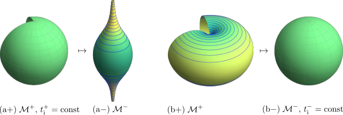
Moreover, to visualize the effect of the Penrose junction condition (11) as a null cone mapping, which was schematically illustrated in figure 1, we plot its explicit realization for the one string case (43), see figure 6.

The above one-string situation can be non-trivially extended by its boosting in the perpendicular direction. The corresponding complex mapping can be constructed as a series of string creation along axis, perpendicular rotation, boost, and final backward rotation, namely
| (45) |
It explicitly becomes
| (46) |
The boost-induced asymmetry reflected in the deformation of the natural static spherical initial conditions, with or being constant, respectively, is visualized in figure 7.
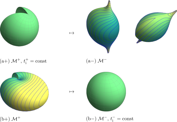

Finally, as a comprehensive picture characterizing the dynamical structure of boosted one-string impulsive spacetime with (46) we plot a sequence of deformations of an initially static swarm of particles. Their initial space and time displacement in the region is chosen in such a way that they all emerge simultaneously in the region as a sphere of constant radius , i.e, it is described by figure 7 (b). Subsequently, due to the non-trivial impulsive effect, the particles start moving along geodesics (straight lines) in the Minkowski background (21) with initial data given by (22) and (23), see figure 9. The vertical deformation and particle acceleration along the axis are given by their attraction by the moving ends of the snapped string. Near poles, where the string ends are attached to the impulsive sphere, the magnitude of velocity approaches the speed of light. The attractive effect of the string ends results in the caustics formed by a mutual crossing of trajectories starting on opposite sides of the initial sphere with respect to the axis. Moreover, the horizontal asymmetry is induced by the boost of the string in the direction. To emphasize the boost effect we plot the cut by plane in the left part of figure 9.

The above discussion shows the effects of a moving snapped cosmic string on free test observers and the way how these effects can be understood and visualized. Notice that the subcase without string boost was already studied in [25, 26] considering also cosmological backgrounds. In the subsequent section, we follow [17, 24] and analyze various impulses generated by a pair of snapped strings in the same way as in the one-string case.
Naturally, in the case of boosted string one can be worried by the fact that the cut out planes are not extrinsically flat, as can be seen in figure 7. However, it can be analytically shown that following situations are equivalent:
6 Two strings geometries
Here, we review and extend the results presented in [24] and discuss their geometric properties via analysis of induced geodesic motion. Subsequently, an alternative sequences of basic steps entering the two strings complex mapping construction will be employed and particular differences in the resulting motion identified.
6.1 Original results by Podolský and Griffiths
The possibility of expanding impulse generated by a colliding and snapping pair of cosmic strings was originally anticipated by Nutku and Penrose in [17]. Simultaneously, there were doubts that explicit realization of the corresponding function is hard to find, however, its existence should be guaranteed by the Riemann theorem. Surprisingly, a few years later Podolský and Griffiths explicitly performed such a construction in [24]. Their simplest non-boosted two-string formula reads
| (47) |
In terms of fixed Cartesian coordinates, it can be described in such a way that the string parameterized by and placed along the axis is rotated to take a place along the axis and the second string (encoded in ) is then created along the axis. However, the construction should be more precisely understood in terms of the active Lorentz transformations (13). This can be seen from the no string limit of (47). Taking both parameters trivial, namely , does not provide the identity, but
| (48) |
which is exactly the residual rotation employed within construction of (47). The Schwarzian derivative (10) is vanishing and the seemingly non-trivial position shift (22) directly shows the unphysical rotation or the artificial identification of the background Cartesian frame. However, to directly gain all relevant information about test particles interacting with the impulse from the refraction formulas (22) and (23), it is important and useful to remove such a coordinate discrepancy. Before we do that, let us show the ultimate result of [24] adding a boost to the simplest interaction of static strings (47), and therefore, interpreted as the collision of strings that induces their snap and subsequent creation of the impulse. The particular complex mapping reads
| (49) |
with
| (50) |
Now, to improve the artificial coordinate effect in (47), and subsequently also in (49), let us perform the following sequence of mappings, namely
| (51) | ||||
| (52) | ||||
| (53) | ||||
| (54) | ||||
| (55) | ||||
| (56) |
These operations can be geometrically understood in terms of the Riemann sphere, see figures 10 and 11 for the special cases, while the fully general mapping takes the form
| (57) |
which naturally becomes identical for trivial boosts and deficit angles, i.e., and . The simplest static interaction of the strings is then described by choosing in (57) which then corresponds to (47) with the artificial coordinate rotation removed, namely
| (58) |
while for a specific choice of boosts we may obtain an improved version of (49). On a general level, the location of ends of the strings for (57) is given by
| (59) |
Here, let us also emphasize that the elementary operation , see (55), which creates the second string placed along -axis, inherently shifts the position in the -direction of the already existing string. In figure 10, this corresponds to the step , where the sphere is distorted and the existing string is effectively boosted in the -direction. We can counterbalance this effect by additional boost in the opposite direction, namely
| (60) |
and , see figure 11 and changes in the sequence . The resulting nodal points are then aligned with the axes and there is no transversal velocity (as could be seen from their action on test particles). These situations are also compared in figure 13.
This discussion is connected with the real location of the strings viewed from the region behind the wave. Geometrically, after cutting out two wedges (deficit angles) we are glueing the corresponding ‘lips’ back together, however, it is done in a particular order. Here, the string governed by parameter remains straight along the axis, while using (59) the string parts governed by , and lying in the - plane, can be identified by the polar angle , namely
| (61) |
In the case with (60) and , i.e., the constants are set so that there is no transversal motion of the strings, pieces of one string are attached to the north and south pole, respectively, while the second string ends form the mutual angle
| (62) |
which is found as a direct application of the general formula (61).


Finally, based on the geodesic motion let us describe the effect of an impulse generated by (58). We visualize its interaction with initially static test particles prepared in to emerge synchronously on a sphere in , see figure 12 identifying the initial data and figure 14 depicting the overall deformation caused by the impulse. The shape evolution corresponds to the straight motion on a flat background. However, there is a non-trivial distribution of velocities given by (23). The map of velocity magnitude,
| (63) |
with
| (64) |
is plotted in figure 15, which again indicates the string ends since in their neighbourhood the test particles approach the speed of light.
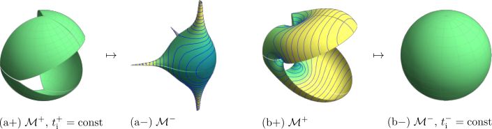


6.2 Peculiar form of the simple two-string mapping
In this part, let us show an alternative construction of the function in the case of a pair of cosmic strings, which should demonstrate the subtlety of the construction process.
Let us start with the sequence of elementary steps
| (65) | ||||
| (66) | ||||
| (67) | ||||
| (68) | ||||
| (69) |
which leads to the mapping
| (70) |
Surprisingly, we identify only three string ends located at
| (71) |
The sequence (65)–(65) thus cuts out the wedge along axis and performs a boost, makes rotation about axis, applies another string-like cut parameterized by along the original axis with another boost, and finally rotates backwards about unchanged axis. The simplified construction is visualized in figure 16. The mapping then leads to identity for and .

Similarly to in the previous section and the case of mapping (57), the second string creation induces an additional boost. Then the edges of Riemann sphere cutouts, parameterized by , represent a generic curved surface. The corresponding extrinsic curvature vanishes and the surface becomes a plane if the inherent boost is compensated by a suitable choice of the artificial boosts in our construction. In particular, taking
| (72) |
guarantees that the strings do not move in the transverse direction at all. This is illustrated in figure 18.
Based on the construction with two string-like operations, one would expect that it describes a pair of perpendicular cosmic strings with four moving ends after their snap. However, inspecting (71) related to the static initial data choice in figure 17, we may conclude that there are only three string pieces. This is exactly the above-mentioned subtlety in the construction. One part of the first string disappears by the creation of the second string (68) which removes the associated nodal point of the Riemann sphere, see in figure 16.
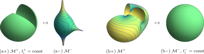

Finally, we can visualize the kinematic effect of the impulse generated by (70) with on the motion of initially static test observers, see figure 19 for the evolution picture and figure 20 for the velocity magnitude distribution. Due to the absence of a string piece along the negative axis and non-compensated inherent boost the resulting picture is asymmetric. Without an appropriate global view, one may be confused. In particular, restricting the analysis to just a quarter of the picture including two perpendicular string pieces in the positive and directions, and taking the deficit parameters one would expect a symmetric picture in the presumed case of a pair of complete strings with four ends. However, we observe an induced motion of test particles that prefers the single-end direction.


6.3 Two parallel strings
As a last example let us briefly show describing two parallel strings. By the definition, they cannot be made standing simultaneously. Therefore, the straightforward idea is to create the first (generically boosted) string, apply the rotation and another boost to induce its motion in the perpendicular direction, rotate back and create the second parallel string again with a generic boost. The relevant sequence in terms of elementary operations is
| (73) |
with the string ends given by
| (74) |
The mapping (73) could be analysed in the same way as in two previous cases. Here, we only show the effect of such a mapping in terms of the Riemann sphere and deformation of the related spherical initial data, see figure 21.

The physical interpretation of the above construction (73) can be directly deduced from the resulting motion of initially static test particles, see figure 22. The deformation is again induced by the dragging of geodesics due to the motion of the string ends.

7 Conclusions
We studied geometries representing expanding impulsive gravitational waves. Our main aim was a geometric description and physical interpretation of the complex mapping entering the Penrose junction conditions (11). In particular, situations related to the string-like nature of the wave source were elaborated. The properties and its refractive effects were connected with the motion of free test particles crossing the null wave surface. This was possible due to employing the recent rigorous results on the geodesic motion in expanding impulses. To clarify the role of elementary steps in construction, we analyzed specific initially static classes of geodesic congruences. Such an approach was introduced in the case of boosted one-string as the simplest possibility. Subsequently, it was followed by three situations with two strings, where we clarified and extended previous results. In particular, we studied a snapping pair cosmic strings, its degenerate subclass with only three string pieces generating the impulse, and finally, a case of two parallel strings. In general, the effects of expanding impulses generated by snapped cosmic strings acting onto geodesic motion can be described as a dragging of test particles by the string ends and induced motion in their directions. This analysis also showed non-trivial inherent boost-like effects within the construction of the two string scenarios and the way of its compensation.
Acknowledgements
DK acknowledges the support of the Czech Science Foundation, Grant 21-11268S. RŠ was supported by the Czech Science Foundation Grant No. GAČR 22-14791S.
References
- [1] Einstein A 1916 Näherungsweise Integration der Feldgleichungen der Gravitation Sitz. Preuss. Akad. Wiss. Berlin 688–96
- [2] Einstein A 1918 Über Gravitationwellen Sitz. Preuss. Akad. Wiss. Berlin 1 154–67
- [3] Pirani F A E 1957 Invariant formulation of gravitational radiation theory Phys. Rev. 105 1089–1099
- [4] Bondi H 1957 Plane gravitational waves in general relativity Nature 179 1072–1073
- [5] Hulse R A and Taylor J H 1975 Discovery of a pulsar in a binary system Astroph. J. 195 L51–L53
- [6] Abbott B P et al. (LIGO Scientific Collaboration and Virgo Collaboration) 2016 Ofor bservation of Gravitational Waves from a Binary Black Hole Merger Ptwo-stringett. 116 061102
- [7] Abbott B P et al. (LIGO Scientific Collaboration and Virgo Collaboration) 2017 GW170817: Observation of Gravitational Waves from a Binary Neutron Star Inspiral Phys. Rev. Lett. 119 161101
- [8] Robinson I and Trautman A 1960 Spherical gravitational waves Phys. Rev. Lett. 4 431–2
- [9] Robinson I and Trautman A 1962 Some spherical gravitational waves in general relativity Proc. Roy. Soc. A 265 463–73
- [10] Kundt W 1961 The plane-fronted gravitational waves Z. Physik 163 77–86
- [11] Kundt W 1962 Exact solutions of the field equations: twist-free pure radiation fields Proc. Roy. Soc. A 270 328–34
- [12] Stephani H, Kramer D, MacCallum M, Hoenselaers C, and Herlt E 2003 Exact Solutions of Einstein’s Field Equations 2nd ed. (Cambridge: Cambridge University Press)
- [13] Griffiths J B and Podolský J 2009 Exact Space-Times in Einstein’s General Relativity (Cambridge: Cambridge University Press)
- [14] Grosser M, Kunzinger M, Oberguggenberger M, and Steinbauer R 2001 Geometric Theory of Generalized Functions Mathematics and its Applications 537 (Dordrecht: Kluwer)
- [15] Steinbauer R and Vickers J A 2006 The use of generalized functions and distributions in general relativity Class. Quantum Grav. 23 R91–R114
- [16] Penrose R 1972 The geometry of impulsive gravitational waves; in General Relativity, ed. L. O’Raifeartaigh (Oxford: Clarendon Press) 101–15
- [17] Nutku Y and Penrose R 1992 On impulsive gravitational waves Twistor Newsletter 34 9–12
- [18] Hogan P A 1992 A spherical gravitational wave in the de Sitter universe Phys. Lett. Math. A 171 21–22
- [19] Podolský J and Griffiths J B 1999 Expanding impulsive gravitational waves Class. Quant. Grav. 16 2937–46
- [20] Hogan P A 1995 Imploding-exploding gravitational waves Lett. Math. Phys. 35 277–280
- [21] Aliev A N and Nutku Y 2001 Impulsive spherical gravitational waves Class. Quant. Grav. 18 891–906
- [22] Podolský J 2002 Exact impulsive gravitational waves in spacetimes of constant curvature; in Gravitation: Following the Prague Inspiration, ed. O. Semerák, J. Podolský and M. Žofka (Singapore: World Scientific) 205–46
- [23] Podolský J, Sämann C, Steinbauer R, and Švarc R 2016 The global uniqueness and -regularity of geodesics in expanding impulsive gravitational waves Class. Quantum Grav. 33 195010
- [24] Podolský J and Griffiths J B 2000 The collision and snapping of cosmic strings generating spherical impulsive gravitational waves Class. Quant. Grav. 17 1401–13
- [25] Podolský J and Steinbauer R 2003 Geodesics in spacetimes with expanding impulsive gravitational waves Phys. Rev. D 67 064013
- [26] Podolský J and Švarc R 2010 Refraction of geodesics by impulsive spherical gravitational waves in constant-curvature spacetimes with a cosmological constant Phys. Rev. D 81 124035
- [27] Steinbauer R 2014 Every Lipschitz metric has -geodesics Class. Quantum Grav. 31 057001
- [28] Filippov A F 1988 Differential Equations with Discontinuous Righthand Sides (Dordrecht: Kluwer Academic Publishers)
- [29] Cortés J 2008 Discontinuous dynamical systems IEEE Control Systems Magazine 28 36–73
- [30] Podolský J, Sämann C, Steinbauer R, and Švarc R 2015 The global existence, uniqueness and -regularity of geodesics in nonexpanding impulsive gravitational waves Class. Quantum Grav. 32 025003