Walk on Stars: A Grid-Free Monte Carlo Method for PDEs with Neumann Boundary Conditions496Journal: TOGVolume: 42418Price: 15.00DOI: 10.1145/3592398CCS: Mathematics of computing Partial differential equationsCCS: Mathematics of computing Integral equationsCCS: Mathematics of computing Probabilistic algorithms

For any set $A\subset\mathbb{R}^{N}$, we use $\partial A$ and $|A|$ for its boundary and volume, resp. We use $p^{A}$ to denote a probability density function on $A$, and write $x\sim p^{A}$ for a random point $x\in A$ drawn from $p^{A}$. For any point $z\in\partial A$, we use $n_{z}$ for the unit outward normal at $z$. We say $\partial A$ is convex at $z$ if all principal curvatures are positive (relative to $n_{z}$), and nonconvex otherwise. For any point $x\in A$, $\overline{x}(\partial A)\coloneqq\argmin_{y\in\partial A}\left\|y-x\right\|$ is the closest point to $x$ on $\partial A$, and $B(x,r)$ is a ball with center $x$ and radius $r$. We drop arguments for $\overline{x}$ and $B$ when the context is clear. We define the $\varepsilon$-shell around $\partial A$ as $\partial A^{\varepsilon}\coloneqq\{x\in\Omega:\left\|x-\overline{x}(\partial A)\right\|<\varepsilon\}$. Finally, we use $\Delta$ for the negative-semidefinite Laplace operator on $\mathbb{R}^{N}$.

Linear elliptic partial differential equations have broad utility in geometry processing, simulation, graphics, and scientific computing in general. A prototypical example is the Poisson equation

which describes, e.g., the steady-state temperature distribution over a domain $\Omega\subset\mathbb{R}^{N}$. Here $u:\Omega\to\mathbb{R}$ is the unknown solution, and $f:\Omega\to\mathbb{R}$ is a source term, analogous to a heat source or sink. We partition the boundary $\partial\Omega$ into a subset $\partial\Omega_{D}$ where the solution has Dirichlet boundary conditions, i.e., prescribed values $g:\partial\Omega_{D}\to\mathbb{R}$, and a subset $\partial\Omega_{N}$ where it has Neumann boundary conditions, i.e., prescribed derivatives $h:\partial\Omega_{N}\to\mathbb{R}$ in the normal direction $n$. Either subset can be empty, in which case we say the equation has pure Dirichlet or Neumann conditions. A function $u$ is harmonic if it satisfies Equation 1 for $f=0$, i.e., if $\Delta u=0$ on $\Omega$.

A screened Poisson equation adds a constant absorption term $\sigma u$, $\sigma\in\mathbb{R}_{>0}$, modeling a medium that dampens or “cools” the solution:

subject to the same boundary conditions as in Equation 1. One can form more general linear elliptic equations by adding variable diffusion, drift and absorption coefficients to Equation 2—see Sawhney et al. 2022 for a detailed exposition. For simplicity our exposition focuses on the (screened) Poisson equation, though much of the material presented here applies to more general linear PDEs (see Section 7 for further discussion).

The solution $u$ to a linear PDE can be expressed via a boundary integral involving the associated Green’s function and Poisson kernel. Assume for now that $\Omega$ is a watertight domain with smooth boundary $\partial\Omega$, and let $x$ be an evaluation point on the interior of $\Omega$. We first multiply the Poisson equation in Equation 1 with its Green’s function $G^{\Omega}$ and integrate over $\Omega$ to get

Applying integration by parts to the first integral, we have

Applying integration by parts again to the second integral in Equation 3.3 and rearranging terms then yields

From the definition $\Delta G^{\Omega}(x,y)=\delta^{\Omega}_{x}(y)$ we arrive at

This equation determines the solution $u$ at $x$ entirely through the solution values $u(z)$ and normal derivatives $\nicefrac{{\partial u(z)}}{{\partial n_{z}}}$ on the boundary $\partial\Omega$, and the source values $f(y)$ inside the domain $\Omega$. From Equation 1, the Dirichlet and Neumann parts of the boundary have prescribed values $g$ and $h$, resp., while $f$ is specified inside the domain. To use Equation 3.3, we must then determine unknown solution values $u(z)$ on the Neumann boundary $\partial\Omega_{N}$, and unknown derivative values $\nicefrac{{\partial u(z)}}{{\partial n_{z}}}$ on the Dirichlet boundary $\partial\Omega_{D}$.

WoS is a Monte Carlo estimator for Equation 11, which means that it approximates the boundary and interior integrals using random samples of the integrands. WoSt follows the same basic recipe, but for a different version of the BIE. Before discussing these estimators in detail, we first review Monte Carlo integration [Fishman 2006], which is the numerical foundation for both methods.

In lieu of balls, WoSt considers regions that are star-shaped with respect to a point $x$ [Hansen et al. 2020]: any ray cast from $x$ must intersect the region boundary only once. Though in principle any star-shaped subdomain could be used, we use regions $\ssd(x,r)$ given by the component of $B(x,r)\ \cap\ \Omega$ containing $x$, for a particular choice of ball $B$ (see Section 4.4.2). Similar to Equation 1, we partition the region boundary into a Neumann part $\partial\mkern-2.0mu\ssd_{N}\coloneqq\partial\Omega_{N}\cap\partial\mkern-2.0mu\ssd$ with prescribed normal derivatives $\nicefrac{{\partial u}}{{\partial n}}=h$ from Equation 1, and a spherical part $\partial\mkern-2.0mu\ssd_{B}\coloneqq\partial B\cap\partial\mkern-2.0mu\ssd$ (see inset).

Letting $A\coloneqq\ssd$ and $C\coloneqq B$ in Equation 8, the BIE becomes

As with the BIE for WoS (Equation 11), the solution value $u(z)$ is the only unknown in this equation: at points $z\in\partial\mkern-2.0mu\ssd_{N}$ the normal derivative $\nicefrac{{\partial u}}{{\partial n}}$ is given by the fixed Neumann data along $\partial\Omega$, and is not needed at points $z\in\partial\mkern-2.0mu\ssd_{B}$, where $G^{B}(x,z)=0$. Since only one quantity is unknown, estimators for this equation need not branch.

Simonov 2008, and later Ermakov and Sipin 2009, take a parallel approach on domains $\Omega$ with convex Neumann boundaries $\partial\Omega_{N}$. In particular, they use regions formed by intersecting $\Omega$ with a ball $B$ whose radius is the distance to the Dirichlet boundary, $d_{\text{Dirichlet}}\coloneqq\left\|x-\overline{x}(\partial\Omega_{D})\right\|$. Hence, $B$ can contain a subset of the Neumann boundary $\partial\Omega_{N}$. In the convex case, such regions are automatically star-shaped. To handle arbitrary domains, WoSt instead uses visibility information to obtain star-shaped regions even near nonconvex Neumann boundaries (which in general can yield a radius $r\leq d_{\text{Dirichlet}}$), as we will see in Section 4.4.2.

At a high level, each step of WoSt accumulates contributions from the Neumann data $h$ and source term $f$. For mixed Dirichlet-Neumann problems, the walk terminates in $\partial\Omega^{\varepsilon}_{D}$, using the Dirichlet data $g$ as the solution estimate, i.e., $\widehat{u}(x_{k})\coloneqq g(\overline{x}_{k}(\partial\Omega_{D}))$. For pure Dirichlet problems, WoSt reduces to WoS; for pure Neumann problems we apply Tikhonov regularization (Section 3.4.2). We first discuss how to sample the next step $x_{k+1}$ (Section 4.4), followed by sampling procedures for $h$ and $f$ (Sections 4.5, 4.6).

The next walk location is importance sampled from the Poisson kernel for a ball centered at the current point $x_{k}$, i.e., $x_{k+1}\sim p^{\partial\mkern-2.0mu\ssd}=P^{B}(x_{k},x_{k+1})$. For a Poisson equation in $\mathbb{R}^{3}$, this kernel is given by

We can use the same sampling density for a screened Poisson equation, since its corresponding kernel simply multiplies $P^{B}$ by a constant in $[0,1)$ determined by the absorption coefficient (Equation 39).

Equation 19 coincides with the signed solid angle subtended by $\partial\mkern-2.0mu\ssd$ at $x_{k+1}$ with respect to $x_{k}$ [Barill et al. 2018; Feng et al. 2023]. In rendering, this term appears in the light transport equation (LTE) [Pharr et al. 2016, Equation 14.15]. Unlike the BIE, the LTE multiplies $P^{B}$ with a binary visibility $V(x,y)$ that equals 1 if $x$ and $y$ are mutually visible. Visibility ensures the product $V(x_{k},y)\ P^{B(x_{k},r)}(x_{k},y)$ is nonnegative: positive if $y$ is visible from $x_{k}$; zero otherwise. Through a change of variables, this product can be importance sampled via directional sampling, i.e., cast a ray from $x_{k}$ in a direction $v\sim\smash{p^{\mathbb{S}^{N-1}}(v)}=\nicefrac{{1}}{{|\mathbb{S}^{N-1}|}}$ uniformly sampled from the unit sphere, and find its first intersection with $\partial\mkern-2.0mu\ssd$:

We refer to Veach and Guibas 1995b for details on the relationship between area sampling and directional sampling.¹¹ 1 If $x_{k}$ lies on the boundary, then the ray origin should be offset slightly along the inward boundary normal to avoid self-intersections; see Wächter and Binder 2019.

For problems with nonzero Neumann conditions, we must evaluate the second term in Equation 18. To do so, we sample a point $z_{k+1}$ uniformly on the Neumann boundary $\partial\Omega_{N}$, adding a contribution $h(z_{k+1})$ only if $z_{k+1}$ is also contained in $\partial\mkern-2.0mu\ssd_{N}$. (Appendix D explains why this term is not estimated using the next location $x_{k+1}$.) This estimate remains unbiased, since we effectively integrate the same function ($h$ restricted to $\partial\mkern-2.0mu\ssd_{N}$) over a larger domain. Sampling the entire Neumann boundary leads to high variance in the estimator, as most samples will not lie on $\partial\mkern-2.0mu\ssd_{N}$. Likewise, rejection sampling is prohibitively expensive since $\partial\mkern-2.0mu\ssd_{N}$ can be much smaller than $\partial\Omega_{N}$. In Section 5.2, we hence describe a strategy for efficiently generating samples $z_{k+1}$ close to $x_{k}$, which significantly reduces variance.

Finally, we sample a point $y_{k+1}\in B(x_{k},r)$ to estimate the interior integral in Equation 18 (Algorithm 4.4.3, lines 24-27). We reuse the

ray direction $v$ we sampled to generate $x_{k+1}$ (Equation 20), and set $y_{k+1}\coloneqq x_{k}+t_{\text{source}}v$, where we sample the distance $t_{\text{source}}\sim p(t_{\text{source}})\propto G^{B}(x_{k},x_{k}+t_{\text{source}}v)$. If the sampled distance $t_{\text{source}}$ is greater than the distance $t_{\partial}\coloneqq\left\|x_{k+1}-x_{k}\right\|$, then the point $y_{k+1}$ is outside the star-shaped region $\ssd(x_{k},r)$, and we reject it (see inset). As in Section 4.4.4, (re)using a hemispherical direction cancels $\alpha(x_{k})=1/2$ when $x_{k}\in\partial\Omega_{N}$.

Our final WoSt estimator is defined recursively as:

where the next walk location $x_{k+1}$ in $\Omega$ or on $\partial\Omega_{N}$ is sampled using the procedure in Section 4.4, and the non-recursive Neumann and source contributions $\widehat{N}$ and $\widehat{S}$ are provided in Algorithm 4.4.3, lines 23 and 27, resp. This estimator maintains the general structure of a WoS estimator, and thus introduces little implementation overhead.

The silhouette of a triangle mesh relative to a given direction $v$ occurs along a set of edges $e$ that satisfy a local silhouette condition. In particular, $e$ is a silhouette edge if for each distinct pair of triangles containing $e$,

where $n_{1},n_{2}$ are consistently oriented normals (see inset). Note in particular that every boundary edge is a silhouette edge. In WoSt, $v$ is the direction from the current walk location $x$ to its closest point on $e$. A naïve strategy for finding the closest silhouette edge is to use a BVH to locate the closest point to $x$ on all edges, skipping edges not contained in the silhouette. However, this strategy is highly inefficient when BVH nodes contain large, finely-tessellated regions that are all front- or back-facing (Figure 11): here each edge is examined (and rejected) exhaustively, whereas ideally the whole node should simply be culled.

Recall that for problems with nonzero Neumann conditions, we sample points from $\partial\Omega_{N}$ (Section 4.5). To increase the likelihood that these points lie on $\partial\mkern-2.0mu\ssd_{N}(x)$, we adopt a hierarchical importance sampling strategy used in rendering to accelerate next-event estimation [Estevez and Kulla 2018]. In particular, during each step of BVH traversal we select only a single random child whose AABB intersects $\ssd(x)$. To give preference to nodes closer to the query point $x$, we sample according to the free-space Green’s function $\smash{G^{\mathbb{R}^{N}}}$ (Algorithm E, lines 12-27), rather than the Green’s function for a ball (which becomes negative outside $\ssd(x)$). Once we reach a leaf node, we uniformly sample a point from the leaf triangles with respect to surface area (see Algorithm E, lines 2–9 and Algorithm E, line 6–10). This point is not guaranteed to lie on $\partial\mkern-2.0mu\ssd_{N}$, but is much more likely to do so compared to uniformly sampling all of $\partial\Omega_{N}$. Estevez and Kulla 2018 describe further improvements to this traversal strategy.

Like WoS, WoSt terminates walks in an $\varepsilon$-shell $\partial\Omega_{D}^{\varepsilon}$ around the Dirichlet boundary, yielding a small, controllable amount of bias. The performance-bias tradeoff is also relatively insensitive to the parameter $\varepsilon$. See Binder and Braverman 2012 and Sawhney and Crane 2020 for more detailed analysis and experiments.

The minimum radius parameter $r^{\min}$ from Section 4.4.3 also incurs bias near concave parts of $\partial\Omega_{N}$. Figure 13 examines the effect of this parameter—compared to $\varepsilon$, $r^{{\min}}$ typically exhibits a more sensitive performance-bias tradeoff, but with run-time improvements again outweighing the small increase in bias. In all other experiments we scale models to fit in a unit sphere, and use $\varepsilon=r^{\min}=0.001$. Adaptively picking $r^{\min}$ based on local boundary curvature may yield even better performance/lower bias.

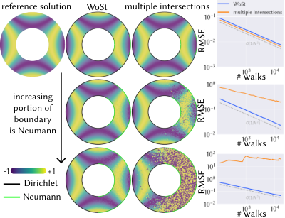
As with most Monte Carlo estimators, WoSt exhibits error of magnitude about $O(1/\sqrt{N})$ with respect to the number of walks $N$ (Figure 14), suggesting that any bias has little impact on overall accuracy. In general we observe that variance tends to be higher (but still predictable) in regions dominated by Neumann boundaries, due to longer walk lengths.

WoSt is both significantly faster and less biased than previous Monte Carlo approaches for solving mixed boundary-value problems with comparable parameter settings. For instance, Figure 16 compares several methods using comparable parameters: a minimum star radius $r^{\min}=0.001$ for WoSt, reflection offset $\zeta=0.01$ for WoS, and step size $l=0.0001$ for the SDE-based method. As discussed inSection 3.4.2, WoS with boundary reflections suffers from bias buildup due to long walks that stick to the Neumann boundary. Methods based on reflecting SDEs perform even worse [Costantini et al. 1998] (see inset), as they incur bias not only on the boundary, but also in the interior. The naïve estimator from Section 4.4.1, which selects one intersection at random, also exhibits massive error as we increase the size of the Neumann boundary (Figure 14, center right). In contrast to all these methods, the star-shaped regions used by WoSt enable one to take large steps without incurring significant bias.

The solution to a Poisson equation with pure Neumann conditions is determined only up to an additive constant. When we solve such a PDE with WoSt, we observe that high frequency details in the PDE solution are often resolved by the first few steps of a random walk, while the contribution from later steps is closer to constant (Figure 18). As discussed in Section 3.4.2, we use Tikhonov regularization to more effectively handle such problems—Figure 19 shows that this approach provides estimates with less noise and smaller bias even with substantial regularization, while ensuring that walk length is not unbounded. In general the number of steps needed to resolve the solution is problem-dependent—more steps are typically needed when the solution has low-frequency global features.

As noted in Section 1, a key motivation for developing grid-free Monte Carlo methods is to push simulation methods closer to the geometric complexity seen in photorealistic rendering—and in nature. To stress-test WoSt on complex geometry, we mock up three simulation examples here. Importantly, these examples do not aim to model exact physics or make quantitative predictions—we seek only to examine solver performance in the presence of (i) extremely complex geometry and (ii) large Neumann boundary regions, which are ubiquitous in real physical problems.

Heat transfer is a central topic in thermal engineering, with three basic modes: radiation, conduction, and convection. Thermal radiation is well-captured by 1st-order Monte Carlo light transport simulation, whereas conduction and convection involve diffusion, which must be simulated via a 2nd-order method like WoS or WoSt [Bati et al. 2023]. Thermal convection can also include turbulent advection à la Navier-Stokes, which can be solved via WoS [Rioux-Lavoie et al. 2022] but is not considered here.

Inspired by toast-darkening experiments of Myhrvold and Migoya 2017, Figure 1 models heat transfer from a toaster to a piece of bread, represented by a CT scan with 3.9 million boundary elements. To model diffusive convection, we solve a Laplace equation with large and small Dirichlet values on the heating elements and toaster cavity (resp.), and Neumann conditions on the bread. The solution is evaluated at roughly 2 million boundary points, using 1 walk per point for fast preview and 256 walks for the final solution; on average, WoSt takes $0.166\text{\,}\mathrm{m}\mathrm{i}\mathrm{l}\mathrm{l}\mathrm{i}\mathrm{s}\mathrm{e}\mathrm{c}\mathrm{o}\mathrm{n}\mathrm{d}\mathrm{s}$ per point for each walk (Figure 15 plots error versus time). A simple phenomenological model is used to translate surface temperature into color (though more principled models of Malliard browning could be used here [Chen et al. 2019]). We observe a marked difference between the temperature distribution resulting from radiation and convection—emphasizing the necessity of 2nd-order models for accurate thermal predictions.

Figure 20 shows another heat transfer experiment, where Dirichlet conditions induced by solar radiation are used to determine heat absorbed by an ectothermic lizard, modeled via detailed spatially-varying Neumann inflow conditions. Unlike FEM or BEM, where boundary data must be evaluated ahead of time, Dirichlet data is evaluated on demand via sphere tracing [Hart 1996]. Scene geometry is represented by a 1.2 million element boundary mesh (for the lizard) and implicit signed distance functions (for the rocks), highlighting the ability of WoSt to work with mixed boundary representations without global meshing. The solution is evaluated at 285k boundary points using 1024 walks per point, taking on average $0.121\text{\,}\mathrm{m}\mathrm{i}\mathrm{l}\mathrm{l}\mathrm{i}\mathrm{s}\mathrm{e}\mathrm{c}\mathrm{o}\mathrm{n}\mathrm{d}\mathrm{s}$ per point for each walk. As in Monte Carlo rendering (and unlike FEM/BEM), scene setup required no model conversion or meshing—even though data was pulled directly from the internet.

Finally, Figure 5 models oxygen diffusion in the lungs, one of many Laplacian transport phenomena with mixed boundary conditions [Grebenkov 2006]. We make a simplification by using Neumann rather than Robin boundary conditions (which are an important topic for future work—see Section 7). While FEM can solve such problems, meshing is both a major performance bottleneck and a hindrance for end-to-end robustness. In this case, even a state-of-the-art method [Hu et al. 2020] yields badly broken geometry; tweaking parameters to capture the correct geometry incurs a full day of compute time, eliminating any advantage of a fast solve. With WoSt we get feedback reliably and immediately in an output-sensitive fashion, here restricted to a cross section. In particular, we evaluate the solution on a $512\times 512$ grid using 1024 walks per point; WoSt takes on average $0.021\text{\,}\mathrm{m}\mathrm{i}\mathrm{l}\mathrm{l}\mathrm{i}\mathrm{s}\mathrm{e}\mathrm{c}\mathrm{o}\mathrm{n}\mathrm{d}\mathrm{s}$ per point for each walk.