Solitonic self-sustained charge and energy transport on the superconducting cylinder

The charged scalar field in two space dimensions is a very simple yet very useful quantum field theory. It has been studied as a lower dimensional toy model for quantum electrodynamicsalgunlibro, as a constructive laboratory to investigate the properties of solitonic solutions in gauge field theories elindioese and, most importantly, in the condensed matter realm, as the effective Ginzburg-Landau theory describing a two-dimensional $s$-wave superconductorginzburglandau.

In the last context, the charged scalar represents the degrees of freedom of the superconducting condensate. The homogeneous solution with a non-vanishing scalar expectation value is interpreted as the superconducting state, since it spontaneously breaks the $U(1)$ charge invariance. Static inhomogeneous solutions then represent excitations; a well known example of which is the Nilsen-Olesen vortexnilsenolesen, which depicts an Abrikosov vortex on the superconducting background abrikosov.

Understanding the dynamics of such excitations requires the inclusion of time derivatives in the scalar field equations of motion. First order time derivatives result in the time-dependent Ginzbug-Landau theorytdginzburglandau1; tdginzburglandau2. This model is non-invariant under time reversal and then it results in dissipation. Alternatively, a Lorentz covariant approach has been suggested, in which the dynamics corresponds to $(2+1)$-dimensional scalar electrodynamicsholandos. It has the advantage of being consistent with the covariance of Maxwell equations, as well as providing a finite penetration depth for the electric fieldhirsch. Dissipation due to non-condensed electrons can then be included through a Rayleigh dissipation function grigorishin.

Recently, unconventional high T_c superconductivity has been observed in twisted bilayer graphenenature, when the twist is adjusted at the so called “magic angle” $\sim 1.1^{\circ}$ at which the fermionic dispersion relation develops a flat bandflatband1; flatband2. It is not clear yet what is the symmetry of the resulting wave function. It has been argued that singleswave1 and multilayerswave2 graphene might form $s$-wave pairs, of which some experimental evidence has been foundswave3.

In the present paper, inspired in the above considerations, we explore the solutions to $(2+1)$-dimensional scalar electrodynamics. We are interested in long-standing time-dependent configurations. Hence, the Ansatz must be chosen in such a way as to minimize all possible sources of dissipation. We find a traveling non-linear wave that moves along the non-compact direction of a cylinder, at the speed of light. We interpret it as an excitation propagating in the superconducting state of a nanotube constructed out of twisted bilayer graphene.

A particularly interesting problem is whether the energy and charge transport can be self-sustained. In other words: is an external field necessary to keep these excitations alive, or is it enough to consider the electromagnetic field generated by the excited charges themselves? Such a question is notoriously difficult (see self1; self2; self3 and references therein) since it entails to consider the back-reaction of the excitations on the electromagnetic field and viceversa. Our construction shows that, at least in the present setting, the second possibility is a viable option.

The paper is organized as follows: In Section II we define our model and parametrize the fields. In Section III we investigate the decoupling conditions which minimize dissipation. In Section IV we write the explicit solution and sections V and VI are dedicated to the study of its transport and topological properties. In Section VII we discuss some specific examples. In Section VIII, we analyze the stability of a special type of perturbations. Finally, in Section IX we discuss our findings.

The effective degrees of freedom of a relativistic $s$-wave superconductor are described in a Lorentz covariant way by standard scalar electrodynamics in $2+1$ dimensionsholandos; grigorishin, which couples a charged scalar field $\Psi$ to the electromagnetic field $A_{\mu}$ minimally, according to the action

$$S=-\frac{1}{2}\int_{\Omega\times\mathbb{R}}d^{3}x\sqrt{-g}\left((D_{\mu}\Psi)^{*}D^{\mu}\Psi+\frac{\gamma}{2}\left(|\Psi|^{2}-\nu^{2}\right)^{2}+\frac{1}{2}F_{\mu\nu}F^{\mu\nu}\!\right)\,,$$

(1)

where the system is defined in a spatial manifold $\Omega$, being $D_{\mu}=\partial_{\mu}-ieA_{\mu}$ the covariant derivative, $e$ the scalar electric charge, $\gamma$ its coupling constant, and $\nu$ its vacuum expectation value.

We parametrize the scalar in the most general way, as

$$\Psi=he^{ieG}\,,$$

(2)

where the factor of $e$ in the exponent is introduced for later convenience. Regarding the gauge field, we use a “Clebsch representation” of the form

$\displaystyle A_{\mu}=\partial_{\mu}\Lambda+\lambda\,\partial_{\mu}F\,,$

(3)

in terms of the “Clebsch potentials” $\Lambda$, $\lambda$ and $F$. In $2+1$ dimensions this decomposition is completely general and does not restrict the fields in any sense. Of course the gradient part $\partial_{\mu}\Lambda$ can be adjusted to any desired value by a gauge transformation, but we leave that for later after deriving the equations of motion.

Since the parametrization is not restrictive, we can safely plug it into the action and then obtain the equations of motion by varying $h,G,\Lambda,\lambda$ and $F$. To do that, we need the expressions for the gauge curvature and the covariant derivative

	$\displaystyle\!\!\!\!\!\!\!\!F_{\mu\nu}=\partial_{\mu}\lambda\partial_{\nu}F-\partial_{\nu}\lambda\partial_{\mu}F\,,$		(4)
	$\displaystyle\!\!\!\!\!\!\!\!D_{\mu}\Psi=\left(\partial_{\mu}h+ieh(\partial_{\mu}G-\partial_{\mu}\Lambda-\lambda\partial_{\mu}F)\right)e^{ieG}\,,$		(5)

which, together with Eqs. (2) and (3), result in the rewritten form of the action

$$S=\frac{1}{2}\int_{\Omega\times\mathbb{R}}d^{3}x\sqrt{-g}\left(-(\partial h)^{2}-{e^{2}}(\partial G-\partial\Lambda-\lambda\partial F)^{2}h^{2}-\frac{\gamma}{2}\left(h^{2}-\nu^{2}\right)^{2}+(\partial\lambda\cdot\partial F)^{2}-(\partial\lambda)^{2}(\partial F)^{2}\right)\,.$$

(6)

This can be varied with respect to the different fields, to obtain the equations of motion of the system. We start with the scalar phase $G$, obtaining the equation

$$\partial^{\mu}\left((\partial_{\mu}G-\partial_{\mu}\Lambda-\lambda\partial_{\mu}F)h^{2}\right)=0\,.$$

(7)

Notice that the same equation can be obtained by varying with respect to $\Lambda$. Then, we can choose the gauge $\Lambda=G$ and, replacing it into the action, the remaining equations take the form

	$\displaystyle\!\!\!\!\!\!\!\!\!\!\!\!\!\!\!\!\partial^{\mu}\!\left((\partial F)^{2}\partial_{\mu}\lambda-(\partial\lambda\cdot\partial F)\partial_{\mu}F\right)-{e^{2}}\lambda h^{2}(\partial F)^{2}=0\,,$		(8)
	$\displaystyle\!\!\!\!\!\!\!\!\!\!\!\!\!\!\!\!\Box h-e^{2}h\lambda^{2}(\partial F)^{2}-\gamma(h^{2}-\nu^{2})h=0\,,$		(9)
	$\displaystyle\!\!\!\!\!\!\!\!\!\!\!\!\!\!\!\!\partial^{\mu}\left((\partial\lambda\cdot\partial F)\partial_{\mu}\lambda-\left((\partial\lambda)^{2}+{e^{2}}h^{2}\lambda^{2}\right)\partial_{\mu}F\right)=0\,,$		(10)

while Eq. (7) simplifies to

$$\partial^{\mu}\!\!\left(h^{2}\lambda\partial_{\mu}F\right)=0\,.$$

(11)

Equations (8)-(11) constitute the full set of equations of motion of the system.

In the above equations (8)-(11) the electromagnetic variables $F$ and $\lambda$ are coupled among them and to the scalar one $h$. This means that any amount of energy stored on any of the fields will get distributed among all the degrees of freedom as the system evolves. In any realistic situation, each variable is coupled to an external dissipative channel. This implies that the energy will then flow out of the system through all of them. If one waits long enough, it is reasonable to expect that one should be left with a configuration in which all the possible dissipative processes have already happened. Thus, the Ansatz describing such configuration must minimize the coupling among the different dissipative channels: this happens when the different degrees of freedom of the gauge and scalar fields are decoupled. In that case, the energy stored on any degree of freedom dissipates only through the corresponding channel, resulting in less dissipation overall.

These intuitive arguments lead to the following consistent Ansatz. First of all, one needs to impose the “force free” conditions $\partial\lambda\cdot\partial F=\partial h\cdot\partial F=0$ and the “light-like” condition $(\partial F)^{2}=0$, since in this way two degrees of freedom (the gauge field and the amplitude of the scalar field) get decoupled. Then, the additional condition $\partial((\partial\lambda)^{2})\cdot\partial F=0$ must be imposed for consistency. In this way, the full set of coupled field equations is reduced to the decoupled pair

	$\displaystyle\square h-\gamma(h^{2}-\nu^{2})h=0\,,$		(12)
	$\displaystyle\square F=0\,,$		(13)

where we assumed $(\partial\lambda)^{2}+{e^{2}}h^{2}\lambda^{2}\neq 0$. These equations must be solved together with the constraints

	$\displaystyle(\partial F)^{2}=0\,,\qquad\qquad$		(14)
	$\displaystyle\partial\lambda\cdot\partial F=0\,,\;\quad\qquad$		(15)
	$\displaystyle\partial h\cdot\partial F=0\,,$		(16)
	$\displaystyle\partial((\partial\lambda)^{2})\cdot\partial F=0\,,$		(17)

to obtain a full solution of the system.

The next step is to specify the space-time geometry $\Omega\times\mathbb{R}$ in which our fields propagate. We choose a cylinder topology with planar metric

$$ds^{2}=-dt^{2}+dz^{2}+d\varphi^{2}\,,$$

(18)

where the coordinate $\varphi\approx\varphi+L_{\varphi}$ goes around the cylinder, while $-{L_{z}}/{2}<z<{L_{z}}/{2}$ runs along it (the case of a very long cylinder corresponds to $L_{z}\rightarrow+\infty$). We can change to lightlike coordinates $z_{\pm}=(z\pm t)/\sqrt{2}$ obtaining

$$ds^{2}=2dz_{+}dz_{-}+d\varphi^{2}\,,$$

(19)

which implies in the equations of motion

	$\displaystyle 2\partial_{+}\partial_{-}h+\partial_{\varphi}^{2}h-\gamma(h^{2}-\nu^{2})h=0\,,$		(20)
	$\displaystyle 2\partial_{+}\partial_{-}F+\partial_{\varphi}^{2}F=0\,,$		(21)

and in the constraints

	$\displaystyle\!\!\!\!\!\!\!\!2(\partial_{+}F)(\partial_{-}F)+(\partial_{\varphi}F)^{2}=0\,,$		(22)
	$\displaystyle\!\!\!\!\!\!\!\!\partial_{+}\lambda\,\partial_{-}F+\partial_{-}\lambda\,\partial_{+}F+\partial_{\varphi}\lambda\,\partial_{\varphi}F=0\,,$		(23)
	$\displaystyle\!\!\!\!\!\!\!\!\partial_{+}h\,\partial_{-}F+\partial_{-}h\,\partial_{+}F+\partial_{\varphi}h\,\partial_{\varphi}F=0\,,$		(24)
	$\displaystyle\!\!\!\!\!\!\!\!\partial_{+}((\partial\lambda)^{2})(\partial_{-}F)\!+\!\partial_{-}((\partial\lambda)^{2})(\partial_{+}F)\!+\!\partial_{\varphi}((\partial\lambda)^{2})\partial_{\varphi}F=0\,.$

The lightlike condition in the first line can then be solved by first choosing $\partial_{\varphi}F=0$ and then imposing $\partial_{+}F=0$ or $\partial_{-}F=0$. The force free conditions in the second and third lines then imply that $\lambda$ and $h$ should depend on the same $z_{\pm}$ variable as $F$. With these choices, the condition on the last line as well as the equation of motion for $F$ are automatically satisfied. We are then left with only one equation of motion, the one for $h$, which now reads

$$\partial_{\varphi}^{2}h-\gamma(h^{2}-\nu^{2})h=0\ .$$

(26)

This equation corresponds to a quartic oscillator, and can be integrated once to get the first order relation

$$\frac{\left(\partial_{\varphi}h\right)^{2}}{2}-\frac{\gamma}{4}\left({h^{2}}-\nu^{2}\right)^{2}=-\frac{\gamma\nu^{4}}{4}\left(\frac{m-1}{m+1}\right)^{2}\ ,$$

(27)

where the integration constant in the right hand side was conveniently parametrized in terms of a new number $m$. This can reduced to quadratures, as

$$\int\frac{dh}{\sqrt{\left({h^{2}}-\nu^{2}\right)^{2}-\nu^{4}\left(\frac{m-1}{m+1}\right)^{2}}}=\pm\sqrt{\frac{\gamma}{2}}(\varphi-\varphi_{0})\ ,$$

(28)

where $\varphi_{0}$ is a new integration constant. The remaining integral can be performed explicitly.

For the particular case $m=1$ we get the solution

$$h=\nu\tanh\left(\nu\sqrt{\frac{\gamma}{2}}(\varphi-\varphi_{0})\right)\ ,$$

(29)

where an overall $\pm$ sign was removed by a gauge transformation. Is is evident that this function approaches the vacuum value at $\varphi\to\pm\infty$. This implies that the natural boundary condition, namely that the Higgs field matches its vacuum value at the boundary of the sample, can only be satisfied in an infinite plane.

If $m\neq 1$ the solution can be written in terms of the Jacobi elliptic sine function, as

$$h=\nu\sqrt{\frac{2m}{1+m}}\,\mathrm{sn}\!\left(\nu\sqrt{\frac{\gamma}{1+m}}\,(\varphi-\varphi_{0}),m\right)\ ,$$

(30)

where again an overall $\pm$ sign was gauged away. In this expression, in order to have a real $h$ we need a positive value for $m$. Since the solution is invariant when $m\to 1/m$, we only need to consider $0<m<1$. Here and accordingly to the constraint $\partial_{+}h=0$ or $\partial_{-}h=0$, the integration constants $m$ and $\varphi_{0}$ are arbitrary functions of $z_{-}$ or $z_{+}$, respectively. These will be restricted further as we impose physically meaningful boundary conditions on the obtained solution.

If the solution is defined on a tube, then the value of $h(\varphi)$ must differ from the value $h(\varphi+L_{\varphi})$ by a gauge transformation, i.e. by a phase. Since $h$ is real, the only possible phase is an overall sign $\pm$, implying a periodic or antiperiodic solution. This imposes

$$\nu\sqrt{{\gamma}}\,L_{\varphi}=2n\sqrt{(1+m)}K(m)\ ,$$

(31)

where $n\in\mathbb{Z}$ is an arbitrary integer and $K(m)$ is the complete elliptic integral of the first kind. Then $m$ is fixed to a constant value independent of $z_{\pm}$. For the model parameters satisfying $\nu\sqrt{\gamma}\,L_{\varphi}>\pi n$, this equation has a non-trivial solution; see Fig. 1. The solution is periodic for $n$ even and antiperiodic for $n$ odd.

If instead we want to define the solution on a ribbon extending from $\varphi_{0}$ to $\varphi_{0}+L_{\varphi}$, we need to impose that the Higgs field reaches its vacuum expectation value at the edges $h(\varphi_{0})=\pm h(\varphi_{0}+L_{\varphi})=\nu$. It has to do it smoothly, thus we also need to satisfy $h^{\prime}(\varphi_{0})=\pm h^{\prime}(\varphi_{0}+L_{\varphi})=0$. This is just a particular case of the (anti)periodicity conditions discussed in the previous paragraph, and imposes the same quantization condition for $m$. However, since the overall factor satisfies $\sqrt{2m/(1+m)}<1$ for the allowed range of $m$, the value of $h$ is never $\pm\nu$, implying that the solution cannot exist on a ribbon.

Notice that the solution (30) changes sign $n$ times as the variable $\varphi$ goes around the tube. This can be made explicit by writing

$\displaystyle h=\left|h\right|e^{i\left[\frac{n\pi\varphi}{L_{\varphi}}\right]}\,,$

(32)

where $[\cdots]$ stands for the integer part. The exponent is then a discontinuous function, which jumps as $\varphi$ grows. However, a smooth overall phase for the Higgs field $\Psi$ can be obtained by choosing the function $G$ in our Ansatz (2) in the form

$$eG+\left[\frac{n\pi\varphi}{L_{\varphi}}\right]=\frac{n\pi\varphi}{L_{\varphi}}\,.$$

(33)

With this form of $G$, the number $n$ is measuring the winding of the Higgs phase around the cylinder.

The full solution of the system then reads

	$\displaystyle\!\!\!\!\!\!\!\!\!\!\!\!\!\!\!\!\!\!\!F=F(z_{\pm})\,,$		(34)
	$\displaystyle\!\!\!\!\!\!\!\!\!\!\!\!\!\!\!\!\!\!\!\lambda=\lambda(z_{\pm},\varphi)\,,$		(35)
	$\displaystyle\!\!\!\!\!\!\!\!\!\!\!\!\!\!\!\!\!\!\!h=\nu\sqrt{\frac{2m}{1+m}}\,\mathrm{sn}\!\left(\nu\sqrt{\frac{\gamma}{1+m}}\,(\varphi-\varphi_{0}),m\right)\ ,$		(36)
	$\displaystyle\!\!\!\!\!\!\!\!\!\!\!\!\!\!\!\!\!\!\!eG=\frac{n\pi\varphi}{L_{\varphi}}-\left[\frac{n\pi\varphi}{L_{\varphi}}\right]=e\Lambda\,,$		(37)

where $m$ is quantized as in Fig. 1 with $n\in\mathbb{Z}$, and the functions $F(z_{\pm})$, $\varphi_{0}(z_{\pm})$ and $\lambda(z_{\pm},\varphi)$ are chiral but otherwise completely arbitrary, being determined by the initial conditions.

The electric current of the above solution can be written as twice the coefficient of the gauge potential $\lambda\partial_{\pm}F$ in the action, and it takes the form

	$\displaystyle J_{\pm}={-}e^{2}h^{2}\lambda\partial_{\pm}F\,,$		(38)
	$\displaystyle J_{\varphi}=0\,,$		(39)

implying $J_{t}=\pm J_{z}=\pm J_{\pm}$. Here and along this section, the top (respectively bottom) signs represent the solution that depends on $z_{+}$ (respectively $z_{-}$). The above result implies in particular that, in order to have a well defined current, the function $\lambda(z_{\pm},\varphi)$ has to be periodic in the variable $\varphi$.

We can also calculate the electromagnetic field strength, which read

	$\displaystyle F_{\varphi\pm}=\partial_{\varphi}\lambda\,\partial_{\pm}F={-}\partial_{\varphi}(J_{z}/e^{2}h^{2})\,,$		(40)
	$\displaystyle F_{\pm\mp}=F_{\pm\pm}=0\,,$		(41)

or in other words

$$E_{z}=0\ ,\quad-B=\pm E_{\varphi}\equiv F_{\varphi\pm}\ .$$

(42)

This results on a vanishing total magnetic flux $\Phi_{B}$ on the cylinder, as the integral

	$\displaystyle\Phi_{B}$	$\displaystyle=$	$\displaystyle\int_{\Omega}B=\int d\varphi\,dz\,\partial_{\varphi}\left(\frac{J_{z}}{e^{2}h^{2}}\right)=$		(43)
		$\displaystyle=$	$\displaystyle\int dz\,\left.\frac{J_{z}}{e^{2}h^{2}}\right|_{\varphi}^{\varphi+L_{\varphi}}=0\,,$

vanishes in virtue of the periodicity of $J_{z}/e^{2}h^{2}$.

Effective electric conductivities can be defined as quotients of the electric current components divided by the electric field ones. This results in an infinite effective direct conductivity $\sigma_{zz}=J_{z}/E_{z}$, and an effective Hall conductivity with value

$$\sigma_{z\varphi}=J_{z}/E_{\varphi}={\mp}e^{2}h^{2}/\partial_{\varphi}\log\lambda\,.$$

(44)

Finally, the components of energy momentum tensor read

	$\displaystyle T_{\pm\pm}=-e^{2}h^{2}\lambda^{2}(\partial_{\pm}F)^{2}-(\partial_{\pm}h)^{2}-F_{\pm\varphi}^{2}\,,$		(45)
	$\displaystyle T_{\pm\mp}=\frac{1}{2}(\partial_{\varphi}h)^{2}+\frac{\gamma}{4}(h^{2}-\nu^{2})^{2}\,,$		(46)
	$\displaystyle T_{\varphi\varphi}=-\frac{1}{2}(\partial_{\varphi}h)^{2}+\frac{\gamma}{4}(h^{2}-\nu^{2})^{2}\,,$		(47)
	$\displaystyle T_{\varphi\pm}=-\partial_{\varphi}h\,\partial_{\pm}h\,,$		(48)

which results on an energy density $T_{tt}=T_{\pm\pm}-T_{\pm\mp}$, implying that for a finite tube of length $L_{z}$ the total energy is finite. Notice that $T_{\varphi\varphi}$ is minus the constant (27), while $T_{\pm\mp}$ is minus the Lagrangian in (6) evaluated on the restrictions (14)-(15) with $G=\Lambda$.

It is important to notice that the field strengths, the electric current, and the energy momentum tensor, are all periodic in $\varphi$, even in the case when $h$ is anti-periodic.

Since our solutions are characterized by an integer $n$ which is a winding number, we may wonder whether it is related to some topological charge. If we write the standard form of the topological charge for $2+1$ scalar electrodynamics as

$$Q=i\int_{\Omega}d\Psi\wedge d\Psi^{*}=i\int_{\partial\Omega}\Psi\wedge d\Psi^{*}\ ,$$

(49)

where $\Omega$ is now our cylinder and $\partial\Omega$ are the two circles at the cylinder ends, we get the explicit expression

	$\displaystyle Q$	$\displaystyle=$	$\displaystyle i\int d\varphi\,\left(\left.\Psi\partial_{\varphi}\Psi^{*}\right|_{z=\frac{L_{z}}{2}}+\left.\Psi\partial_{\varphi}\Psi^{*}\right|_{z=-\frac{L_{z}}{2}}\right)$		(50)
		$\displaystyle=$	$\displaystyle 2n\pi\ .$

Then we see that our solutions are topological in nature, being characterized by a topological charge.

An interesting point is that the charge $Q$ was obtained from the same expression that would result in the topological charge of an Abrikosov-Nielsen-Olesen vortex. Thus, our solutions may in principle be continuously deformed into such a vortex, without changing the value of $Q$.

In static configurations, the presence of a topological charge is often related to the existence of a Bogomol’nyi-Prasad-Sommerfield (BPS) bound on the energy. A natural question is whether something similar may exist for the present time dependent solutions. To check that, we evaluate the on-shell action of the configuration

$$S_{\sf on-shell}=-\int dz_{+}dz_{-}d\varphi\left(\frac{1}{2}(\partial_{\varphi}h)^{2}+\frac{\gamma}{4}(h^{2}-\nu^{2})^{2}\right)\ ,$$

(51)

which can be rewritten as

$$S_{\sf on-shell}\!=\!-\frac{1}{2}\!\int\!dz_{+}dz_{-}d\varphi\left(\partial_{\varphi}h-s\sqrt{\frac{\gamma}{2}}(h^{2}\!-\nu^{2})\right)^{2}\!+P,$$

(52)

where $s=\pm 1$ is a sign, and we have defined the magnitude $P$ according to

$$P=-s\sqrt{\frac{\gamma}{2}}\int dz\,d\varphi\,(h^{2}-\nu^{2})\,\partial_{\varphi}h\ .$$

(53)

In this expression, the integral in $\varphi$ can be explicitly performed, resulting in

$$P=-s\sqrt{\frac{\gamma}{2}}\int dz\,\left.\left(\frac{h^{2}}{3}-\nu^{2}\right)h\right|_{\varphi}^{\varphi+L_{\varphi}}\ ,$$

(54)

this vanishes for periodic ($n$ even) solutions, but not for antiperiodic ($n$ odd) ones. In this last case, the result has the somewhat disappointing feature of being dependent on the value of $\varphi$ where the circle is closed $\varphi\approx\varphi+L_{\varphi}$, which difficults a proper physical interpretation of $P$ as a topological charge. However, we can write the following BPS-like bound

$$S_{\sf on-shell}\leq P\ ,$$

(55)

whose saturation implies the field equations, as expected from a standard BPS bound. Indeed, the above bound is saturated when equation (27) is satisfied, for the particular case $m=1$. As we mention earlier, the corresponding solution (29) does not satisfy the boundary conditions on a tube, and can only be defined on an infinite plane.

In conclusion, the family of solutions we have found on the tube satisfies the bound (55).

In order to get some insight on the behavior of the solutions, we need to specify an explicit form for the arbitrary chiral functions $F(z_{\pm})$ and $\varphi_{0}(z_{\pm})$, and for the function $\lambda(z_{\pm},\varphi)$. We can write Fourier decompositions for all of them, as

	$\displaystyle\!\!\!\!\!\!\!F(z_{\pm})=a_{0}^{F}z_{\pm}+\!\!\sum_{{k^{F}}=0}\!a_{k}^{F}\sin\left(\frac{2\pi k^{F}}{L_{z}}z_{\pm}\!\right)+b_{k}^{F}\cos\left(\frac{2\pi k^{F}}{L_{z}}z_{\pm}\!\right),$
	$\displaystyle\!\!\!\!\!\!\!\varphi_{0}(z_{\pm})=a_{0}^{\varphi}z_{\pm}\!+\!\!\sum_{k^{\varphi}=0}\!a_{k}^{\varphi}\sin\left(\frac{2\pi k^{\varphi}}{L_{z}}z_{\pm}\right)+b_{k}^{\varphi}\cos\left(\frac{2\pi k^{\varphi}}{L_{z}}z_{\pm}\!\right),$
	$\displaystyle\!\!\!\!\!\!\!\lambda(z_{\pm})=a_{0}^{\lambda}z_{\pm}\!+\!\!\sum_{k^{\lambda}=0}\!a_{k}^{\lambda}\sin\left(\frac{2\pi k^{\lambda}}{L_{z}}z_{\pm}\right)+b_{k}^{\lambda}\cos\left(\frac{2\pi k^{\lambda}}{L_{z}}z_{\pm}\!\right),$

where the coefficients $a_{k}^{\lambda}$ and $b_{k}^{\lambda}$ are periodic functions of $\varphi$, and can be decomposed according to

	$\displaystyle\!\!\!\!\!\!\!a_{k}^{\lambda}(\varphi)=\sum_{l=0}a^{\lambda}_{kl}\sin\left(\frac{2\pi l}{L_{\varphi}}\varphi\right)+\tilde{a}^{\lambda}_{kl}\cos\left(\frac{2\pi l}{L_{\varphi}}\varphi\!\right)\,,$
	$\displaystyle\!\!\!\!\!\!\!b_{k}^{\lambda}(\varphi)=\sum_{l=0}b^{\lambda}_{kl}\sin\left(\frac{2\pi l}{L_{\varphi}}\varphi\right)+\tilde{b}^{\lambda}_{kl}\cos\left(\frac{2\pi l}{L_{\varphi}}\varphi\!\right)\,.$

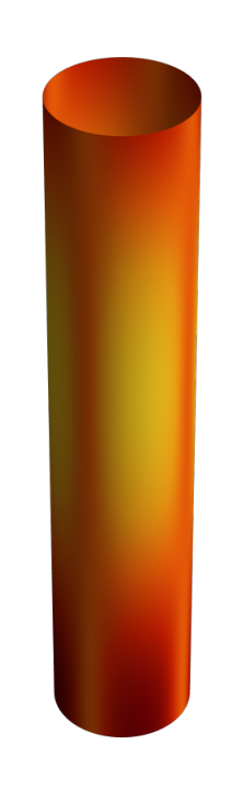
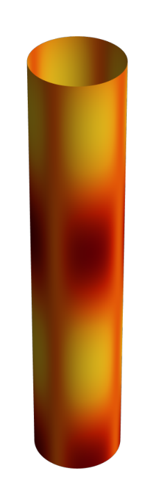
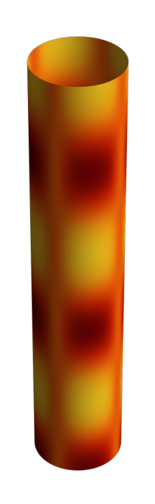
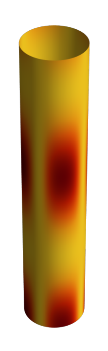
With this expressions, we can plot the profiles of the observable functions, namely the electric current $J_{\pm}$, the energy density $T_{tt}$, and the electromagnetic field $E=\mp B$, for some simple examples, see Figs. 2 to 6.

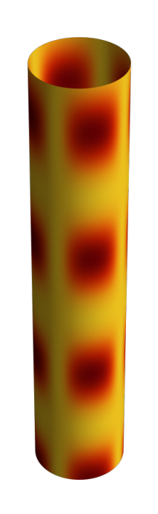
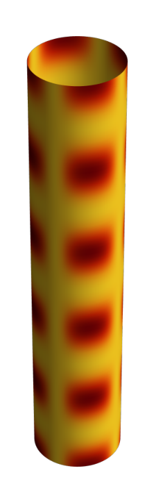
In Fig. 2 we plot some simple configurations with growing values of $n$, which implies a growing number of maxima of the functions around the cylinder. In Fig. 3 we draw some solutions with different values of $k^{\varphi}$, the linear mode controlling the winding of the level curves around the cylinder, the higher modes counting their oscillations along it. Fig. 4 shows configurations with different values of $k^{\lambda}$, which controls the number of maxima of the functions along the cylinder. Fig. 5 shows the some profiles with fixed $k^{\lambda}$ for different values of $l$, which combines with $n$ to tweak the number of maxima around the cylinder. Finally Fig. 6 contains profiles with different values of $k^{F}$, contributing to the number of maxima of the observable functions along the cylinder.

We proved in Section VI that our solutions are characterized by a topological charge $Q=2\pi n$, in which $n$ represent the winding around the cylinder of the phase of the Higgs field. This feature is a proxy for the overall stability of the configuration, since a finite-energy deformation cannot change the winding number. Then, if an instability exists, it must drive the solution into a different one with the same winding number, as for example the Abrikosov-Nielsen-Olesen vortex.

A complete perturbative analysis of the obtained solutions is beyond the scope of the present paper, since it would involve five coupled linear partial differential equations on a non-trivial background. Nevertheless, in this section we analyze a special type of perturbations which have both interesting physical meaning and allow some analytic control: those that preserve the decoupling properties of our Ansatz. Such perturbations are defined by the following small deformations of our Ansatz functions

	$\displaystyle F(z_{\pm})$	$\displaystyle\rightarrow$	$\displaystyle F(z_{\pm})+\varepsilon\,\delta F(z_{\pm})\ ,$		(56)
	$\displaystyle h(\varphi)$	$\displaystyle\rightarrow$	$\displaystyle h(\varphi)+\varepsilon\,\delta h(\varphi)\ ,$		(57)

where $\varepsilon$ is a small dimensionless parameter. These perturbations are very likely to be the smallest energy perturbations of the present exact solutions. The reason is that it takes “a little effort” to perform an angular deformation of $h$ (see, for instance, the discussion of the hedgehog ansatzshifman1; shifman2) as compared to deformations on $h$ depending also on the other coordinates. For this reason the linear operator that determines the spectrum of these perturbations plays a very important role.

The linearized field equations are obtained expanding to the first nontrivial order in $\varepsilon$. They read

	$\displaystyle\partial_{\pm}F\,\partial_{\mp}\delta F$	$\displaystyle=$	$\displaystyle 0\ ,$		(58)
	$\displaystyle-\partial_{\varphi}^{2}\delta h+\gamma(3h^{2}-\nu^{2})\delta h$	$\displaystyle=$	$\displaystyle 0\ ,$		(59)

where $h$ and $F$ are the background solutions.

As far as the equation for the perturbation $\delta F$ is concerned, since $F$ only depends on one of the two light-cone variables $z_{\pm}$ we get that the solution for $\delta F$ must depend on the same light-cone variable

$$\delta F=\delta F\left(z_{\pm}\right)\ .$$

(60)

Thus, imposing reasonable boundary conditions in the $z$-direction, one gets a Fourier expansion for $\delta F$ with real frequencies, so that the perturbation is always well-behaved.

Regarding the perturbation $\delta h$, if we take

$$\delta h=\partial_{\varphi}h\ ,$$

(61)

where $h$ is the background solution satisfying Eq. (26), then $\delta h$ satisfies identically the corresponding linearized field equation in Eq. (58). Moreover, from Eq. (27) it is clear that we can choose the integration constant $m$ close enough to one, in such a way that $\partial_{\varphi}h$ never changes sign: this implies that $\delta h$ has no node. In other words, we have a nodeless zero mode of the linearized field equations. Standard arguments in quantum mechanics then suggest that all the other eigenvalues are positive.

Although the above arguments are not a complete proof of the stability, they suggest that the family of analytic solutions constructed here have interesting physical properties.

We have found exact solutions to $2+1$ scalar electrodynamics, that represent solitonic configurations propagating along a cylinder. The solutions are topological in nature, being indexed by an integer number that counts the winding of the Higgs phase around the cylinder. They are continuously connected to Abrikosov-Nielsen-Olesen vortices. Even if a partial perturbative analysis does not show instabilities, our solutions may in principle relax into vortices via some instability channel we had not considered, or through external dissipation.

There are both a charge density and an electric current along the cylinder, which are equal (up to a sign) and have arbitrary shapes on the cylinder surface. The current is self-sustained since there is no need of an external field to keep it alive. There is no electric current around the cylinder, nor electric field along it. As time runs, the profile moves as a whole along the cylinder, at the speed corresponding to that of the light in the model.

We would like to interpret our solutions as long standing excitations on a superconducting nanotube. As these configurations are independent of the value of the coupling, they can describe both type I and type II superconductors. For this interpretation to work, we need that (1) the superconducting condensate has an $s$-wave symmetryswave1; swave2; swave3, (2) the matter dynamics can be considered relativisticholandos; hirsch; grigorishin, and (3) our two-dimensional fields have to be embedded into a three dimensional setup (this can be done by solving Maxwell’s equation in vacuum and then imposing at the tube radius a suitable set of boundary conditions, that in cylindrical coordinates read $B_{r}=B$, $E_{z}=0$, $E_{\varphi}=\pm F_{\varphi\pm}$). If these hypotheses are fulfilled, the device could in principle be constructed out of twisted bilayer graphene, by compactifying one direction on a certain number of its moiré periods of around $\simeq 13$nm.

N.G. is grateful to Mauricio Sturla, Guillermo Silva and Martin Schvellinger for useful references and insights, and to Universidad de Concepción and Centro de Estudios Científicos for hospitality and support. His work is partially supported by CONICET grants PIP-2017-1109 and PUE084 “Búsqueda de nueva física”, and UNLP grant PID-X791. A. G has been funded by FONDECYT Grant No. 1200293. F. C. has been funded by FONDECYT Grant No. 1200022. J. O. thanks the support of FONDECYT Grant No. 1221504. A. V. has been funded by FONDECYT post-doctoral Grant No. 3200884. The Centro de Estudios Científicos (CECs) is funded by the Chilean Government through the Centers of Excellence Base Financing Program of ANID.

References

- (1) Peskin, M.; Schroeder, D. An Introduction to Quantum Field Theory, Westview Press, 1995.
- (2) Gerard ’t Hooft, Falk Bruckmann Monopoles, Instantons and Confinement, Lectures given at the 5th WE Heraeus Summer School, 1999; arXiv:hep-th/0010225.
- (3) Tinkham, Michael Introduction to Superconductivity, McGraw-Hill, 1996.
- (4) H. B. Nielsen, P. Olesen, Vortex-line models for dual strings, Nuclear Physics B, Volume 61, 1973, Pages 45-61, ISSN 0550-3213.
- (5) A. A. Abrikosov, The magnetic properties of superconducting alloys, Journal of Physics and Chemistry of Solids, Volume 2, Issue 3, 1957, Pages 199-208, ISSN 0022-3697.
- (6) Larkin, Anatoly, and Andrei Varlamov. Theory of fluctuations in superconductors. Vol. 127. OUP Oxford, 2005.
- (7) Kopnin, Nikolai. Theory of nonequilibrium superconductivity. Vol. 110. Oxford University Press, 2001.
- (8) Govaerts, Jan, Damien Bertrand, and Geoffrey Stenuit. On electric fields in low temperature superconductors. Superconductor Science and Technology 14.7 (2001): 463.
- (9) Hirsch, J. E. Electrodynamics of superconductors. Physical Review B 69.21 (2004): 214515.
- (10) Grigorishin, Konstantin V. Extended Time-Dependent Ginzburg-Landau Theory. Journal of Low Temperature Physics 203.3 (2021): 262-308.
- (11) Cao, Y., Fatemi, V., Fang, S. et al. Unconventional superconductivity in magic-angle graphene superlattices. Nature 556, 43-50 (2018).
- (12) Suarez Morell, E., Correa, J. D., Vargas, P., Pacheco, M. & Barticevic, Z. Flat bands in slightly twisted bilayer graphene: tight-binding calculations. Phys. Rev. B 82, 121407 (2010).
- (13) Bistritzer, R. & MacDonald, A. H.Moiré bands in twisted double-layer graphene. Proc. Natl Acad. Sci. USA 108, 12233-12237 (2011).
- (14) Bruno Uchoa and A. H. Castro Neto Superconducting States of Pure and Doped Graphene Phys. Rev. Lett. 98, 146801 (2007).
- (15) Mir Vahid Hosseini and Malek Zareyan, Unconventional superconducting states of interlayer pairing in bilayer and trilayer graphene Phys. Rev. B 86, 214503 (2012).
- (16) E. F. Talantsev, R. C. Mataira & W. P. Crump Classifying superconductivity in Moiré graphene superlattices, Nature Scientific Reports 10, 212 (2020).
- (17) M. Colangeli, A. De Masi, E. Presutti, J Stat Phys (2017) 167:1081–1111.
- (18) T. Kobayashi, M. Kobayashi, Y. Narushima, Y. Suzuki, K. Y. Watanabe, K. Mukai, Y. Hayashi, Phys. Rev. Lett. 128, 085001 (2022).
- (19) B. A. Johnson, K. Brahim, A. G. Balanov, S. Savelev, P. Borisov, Appl. Phys. Lett. 118, 023502 (2021).
- (20) M. Shifman, “Advanced Topics in Quantum Field Theory: A Lecture Course” Cambridge University Press, (2012).
- (21) M. Shifman, A. Yung, “Supersymmetric Solitons” Cambridge University Press, (2009).
- (22) M. B. Green, J. H. Schwarz, and E. Witten, Superstring Theory (Volume 1) (Cambridge University Press, Cambridge, England, 1988).