Kerr black hole in de Sitter spacetime and observational redshift:
Toward a new method to measure the Hubble constant

The KdS line element in the standard Boyer-Lindquist coordinates $\left(t,r,\theta,\varphi\right)$ reads KdS (we use $c=1=G$ units)

with the metric components

where the functions $\Delta_{r}\left(r\right)$, $\Delta_{\theta}\left(\theta\right)$, $\Sigma\left(r,\theta\right)$, and $\Xi$ have the following explicit form

and $M$ is the total mass of the black hole, $a$ is the angular momentum per unit mass $a=J/M$, and $\Lambda$ is the cosmological constant related to dS radius $l_{dS}$ as $\Lambda=3/l_{dS}^{2}$. The KdS metric (2) describes an axially symmetric and stationary spacetime (between the event horizon and the cosmological horizon) that reduces to the standard Kerr black hole in the limit $\Lambda=0$ and the Schwarzschild-dS (SdS) black hole for $a=0$. The coordinate singularities of this spacetime are characterized by $\Delta_{r}=0$ (the four roots correspond to horizons), while calculation of the invariant curvature scalar reveals that the intrinsic singularity is given by $\Sigma=0$ where located at $\left\{r=0,\theta=\pi/2\right\}$ for $a\neq 0$. Therefore, the presence of a cosmological horizon, characterized by the largest root of $\Delta_{r}$, is one of the consequences of non-vanishing $\Lambda$.

In order to find the extreme values of $a$ and $\Lambda$ for having black holes, we found that it is convenient to introduce the normalized variables $x$, $\alpha$, and $\lambda$ as below

and express the $\Delta_{r}$ function in terms of the new variables as follows

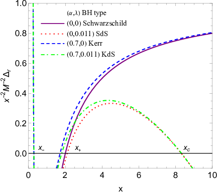
Generally, one can show that $\Delta_{r}$ has (at most) four distinct roots that can be regarded as the cosmological horizon ($x=x_{c}$), the event horizon ($x=x_{+}$), the inner horizon ($x=x_{-}$), and a negative root ($x=x_{0}<0$) so that $x_{-}<x_{+}<x_{c}$ (see Fig. 1). Therefore, we can express $\Delta_{r}$ in terms of these quantities in the following form

Now, by equating the equations for $\Delta_{r}$ given in (11) and (12), the following relations between parameters are found

where $x_{-}$, $x_{+}$, and $x_{c}$ are considered as three fundamental parameters of spacetime. Similar to the Kerr case, there should be a maximum value for the rotation parameter, say $\alpha_{\max}$, such that we have black holes in the range $0\leq\alpha^{2}\leq\alpha_{\max}^{2}$ and a naked singularity for $\alpha^{2}>\alpha_{\max}^{2}$. By considering (13)-(14), and also, the condition $x_{-}<x_{+}<x_{c}$ between roots, we find that the maximum $\alpha_{\max}$ happens whenever $x_{-}\lesssim x_{+}\lesssim x_{c}$, hence all the horizons are closely spaced for $\alpha_{\max}$. Therefore, we should take into account the approximation $x_{-}\approx x_{+}\approx x_{c}$ to obtain $\alpha_{\max}$. On the other hand, $0\leq\alpha^{2}\leq\alpha_{\max}^{2}$ and (13) show that the cosmological constant should obey the following interval as well

Note that in order to have black holes, there is always a maximum cosmological constant, say $\lambda_{\max}$, which corresponds to an arbitrary rotation parameter $\alpha$ in the range $0\leq\alpha\leq\alpha_{\max}$. The maximum value of $\lambda$, in the general case, is corresponding to $\alpha_{\max}$ which is denoted as critical cosmological constant $\lambda_{crit}$ in the aforementioned inequality. Therefore, generally speaking, there is an interval for $\lambda_{\max}$ that depends on the rotation parameter $\alpha$, as $\lambda_{\max}^{(SdS)}(\alpha=0)\leq\lambda_{\max}\leq\lambda_{crit}\left(\alpha=\alpha_{\max}\right)$ so that its lower bound represents the maximum value of $\lambda$ for the SdS black hole and $\lambda\approx\lambda_{\max}^{(SdS)}$ characterizes the near-extremal SdS solution. In other words, there is a maximum value of $\lambda$ for an arbitrary rotation parameter $\alpha$, and similarly, there is a maximum value of $\alpha$ for an arbitrary cosmological constant $\lambda$ (for example, for the SdS black hole with $\alpha=0$, the cosmological constant ranges within $0\leq\lambda\leq\lambda_{\max}^{(SdS)}$).

Now, in order to obtain $\alpha_{\max}$, and then $\lambda_{\max}^{(SdS)}$ and $\lambda_{crit}$, we need to take into account the condition $x_{-}\lesssim x_{+}\lesssim x_{c}$, as we mentioned above. To do so, we first equate Eqs. (11) and (12) while considering $x_{+}$ and $x_{c}$ as two independent variables to obtain the following relations

with $\Pi$ and $\Upsilon$ being

Then, we take into account the near-extremal regime $x_{c}\rightarrow x_{+}$ in the above-mentioned formulas, i.e. when the cosmological horizon $x_{c}$ is very close to the black hole event horizon $x_{+}$ ($x_{c}-x_{+}<<x_{+}$). Hence, we obtain the following relations for $\alpha$, $x_{-}$, $x_{0}$, and $\lambda$ in the nearly extreme regime

where we replaced $\lambda$ with $\lambda_{\max}$ since $x_{c}\approx x_{+}$. Now, the maximum value of the rotation parameter, $\alpha_{\max}$, can be obtained by taking the limit $x_{+}\rightarrow x_{-}$ in the aforementioned relations. By considering $x_{-}\approx x_{+}$ in (24), we obtain a maximum value for the event horizon as below

that is indeed a coincidental point for all the three horizons ($x_{c}\approx x_{+}\approx x_{-}\approx\left(3+2\sqrt{3}\right)/4$), hence it maximizes the rotation parameter in Eq. (23). Therefore, by substituting (27) in (23), we obtain

that is slightly higher than unity for the standard Kerr black hole ($\alpha_{\max}>\alpha_{\max}^{Kerr}=1$). It is worthwhile to mention that this value corresponds to the maximum possible value of the cosmological constant, $\lambda_{crit}\left(\alpha=\alpha_{\max}\right)$, and therefore, it will be less for lower values of the cosmological constant. Thus, the rotation parameter ranges

with $\alpha_{\max}$ given by (28).

Now, we obtain bounds on maximum values of the cosmological constant $\lambda_{\max}$, namely $\lambda_{\max}^{(SdS)}(\alpha=0)$ and $\lambda_{crit}\left(\alpha=\alpha_{\max}\right)$. The maximum value for the event horizon is given in Eq. (27) that corresponds to maximally rotating black holes with $\alpha=\alpha_{\max}$. Therefore, by substituting Eq. (27) in Eq. (26), we obtain $\lambda_{crit}\left(\alpha=\alpha_{\max}\right)=16/\left(3+2\sqrt{3}\right)^{3}$.

On the other hand, since SdS is static $\alpha=0$, we set $x_{-}=0$ in (24) and obtain the maximum value of the event horizon as $x_{+}=3\equiv x_{+\max}^{(SdS)}$ for this case (we set $x_{-}=0$ because SdS black holes have no inner horizon). By replacing this value in Eq. (26), one can find the maximum value of the cosmological constant for the static case as $\lambda_{\max}\left(\alpha=0\right)=1/27\equiv\lambda_{\max}^{(SdS)}$. We summarized the results of this section on the bounds of KdS parameters as follows

with

Therefore, the maximum value of the cosmological constant in the Kerr geometry must be in the aforementioned interval. For instance, the relation of $\lambda$ given in (14) must obey $0\leq\lambda\leq\lambda_{\max}^{(SdS)}$ for the static case $\alpha=0$, while $\lambda=0$ represents the standard Schwarzschild solution and $\lambda\approx\lambda_{\max}^{(SdS)}$ denotes nearly extreme SdS black holes. Other cases far from these two extreme values and within this range are known as SdS black holes while we have a naked singularity for $\lambda>\lambda_{\max}^{(SdS)}$.

On the other hand, one may note that for an arbitrary value of the rotation parameter in the range $1<\bar{\alpha}\leq\alpha_{\max}$, $\lambda$ acquires a minimum value as well and must obey $\lambda_{\min}\leq\lambda\leq\lambda_{\max}$ for a given $\bar{\alpha}$. Obtaining these bounds on the parameters of KdS black holes is important since they will help us to find valid values of the redshifted photons emitted by massive particles orbiting a KdS black hole.

Various regions of KdS black holes in the $\alpha-\lambda$ plane are illustrated in Fig. 2. In this figure, the continuous vertical blue line $\alpha=0$ represents SdS black holes, the continuous horizontal red line $\lambda=0$ shows the standard Kerr black holes, and there are standard Schwarzschild solutions where they join $\left\{\alpha=0,\lambda=0\right\}$. Extreme points $\left\{\alpha=0,\lambda=\lambda_{\max}^{(SdS)}\right\}$ and $\left\{\alpha=\alpha_{\max},\lambda=\lambda_{crit}\right\}$ that we have obtained analytically in (30) are shown on the top corners. To obtain the $\lambda_{\max}$-dashed line on the top of the shaded green area, we used Eqs. (23) and (26) while one can employ the relations (17)-(20) in order to find the $\lambda_{\min}$-dashed line on the right of the shaded green area assuming $x_{-}=x_{+}$. Thus, we derived all the marginal points of KdS black holes in the parameter space $\alpha-\lambda$ analytically that are presented in Eqs. (17)-(20), (23)-(26), and (30). Note that some of these bounds have been found in KdSECO from a different approach.

It is worthwhile to mention that we have a naked singularity for $\lambda>\lambda_{\max}$, whereas for $\alpha>\alpha_{\max}$, the inner and outer horizons vanish and there is just a cosmological horizon assuming $\lambda\neq 0$. One can see that the non-vanishing cosmological constant introduces two important modifications to the standard Kerr geometry: (i) It leads to a new horizon, known as the cosmological horizon, and (ii) allows having higher values for the rotation parameter. As we shall see in Sec. III.1, the cosmological constant also modifies the particles’ motion and leads to an upper bound on the radius of stable emitters in circular motion.

The equation of motion of test massless/massive particles in the rotating spacetimes is described by the geodesic equations. In this regard, the geodesic equations can be obtained by using the separation of variables of the Hamilton-Jacobi equation. The Hamilton-Jacobi equation, for a given background $g_{\mu\nu}\left(x^{\rho}\right)$, leading to the geodesic equations can be written as CarterCons

where $S$ represents Hamilton principal function. In this relation, $\tau$ is the proper time that parametrizes the particle worldline and is related to the affine parameter $\sigma$ by $\tau=\sigma m$ which $m$ is the particle rest mass ($\tau$ represents the affine parameter in the case of photons). For the KdS spacetime, the Hamilton principal function $S$ can be separated as

for both timelike ($\eta=1$) and null ($\eta=0$) particles, and $S_{r}\left(r\right)$ is a function of $r$ while $S_{\theta}\left(\theta\right)$ is a function of $\theta$ only. The constants of motion $\bar{E}$ and $\bar{L}$, respectively, correspond to conserved energy $E_{0}$ and angular momentum $L_{0}$ of massive particles obtained through the following equations

where $\xi^{\mu}=\delta_{t}^{\mu}$ is the timelike Killing vector field and $\psi^{\mu}=\delta_{\varphi}^{\mu}$ is the rotational Killing vector field of the spacetime, and $U^{\mu}$ is the $4$-velocity of particles which is normalized to unity $U^{\mu}U_{\mu}=-1$.

On the other hand, by substituting the decomposition (33) into the Hamilton-Jacobi equation (32), we get the following equality

where the lhs is a function of $\theta$ only and the right-hand side (rhs) just depends on the $r$-coordinate. Therefore, either side is equal to a constant of motion, known as the Carter constant $\mathcal{C}$ with the following form CarterCons

which $\mathcal{K}$ is a constant that arises from the contraction of the Killing tensor field $K_{\mu\nu}$ of Kerr-dS spacetime with the $4$-velocity as $\mathcal{K}=K_{\mu\nu}U^{\mu}U^{\nu}$. Now, by making use of (34)–(37), and the unity condition $U^{\mu}U_{\mu}=-1$, we can obtain the $4$-velocity components of massive particles ($\eta=1$) in terms of constants of motion $\bar{E}$, $\bar{L}$, and $\mathcal{K}$ as follows

where the rhs of Eq. (39) is a function of $r$ and the rhs of Eq. (40) is a function of $\theta$ only. Note that Eqs. (34) and (35) have been used to obtain Eqs. (38) and (41), while Eqs. (36), (37), and the unity condition $U^{\mu}U_{\mu}=-1$ have been employed to get the relations (39) and (40).

From Eq. (40), it is clear that the constant of motion $\mathcal{K}$ [that is related to the Carter constant by Eq. (37)] represents a measure of how much the geodesic of particles deviates from the equatorial plane $\theta=\pi/2$, where this constant vanishes. Therefore, the test particles moving in the equatorial plane have zero $\mathcal{K}$, whereas it is non-vanishing whenever particles cross the equatorial plane.

The first-order differential equations presented in Eqs. (38)-(41) show the geodesic equations of massive particles for every direction in the KdS background in terms of the constants of motion $\bar{E}$, $\bar{L}$, and $\mathcal{K}$. These equations reduce to the corresponding relations given in PRDhn for Kerr geometry in the limit $\Lambda\rightarrow 0$, as it should be. Therefore, the cosmological constant encodes deviations of KdS black holes from the standard Kerr background.

On the other hand, a similar strategy can be followed to obtain the null geodesics of photons with $4$-momentum $k^{\mu}$ moving between the event horizon and cosmological horizon of the KdS spacetime. For massless test particles, the conserved energy $\bar{E}_{\gamma}$ and angular momentum $\bar{L}_{\gamma}$ of particles can be found through the following relations

where the $4$-momentum $k^{\mu}$ of null particles satisfies $k^{\mu}k_{\mu}=0$. Besides, the equality (36) takes the form

for the null particles ($\eta=0$). Now, by making use of Eqs. (42)-(44) and $k^{\mu}k_{\mu}=0$, we obtain the various components of the $4$-momentum in terms of the constants of motion $\bar{E}_{\gamma}$, $\bar{L}_{\gamma}$, and $\mathcal{K}_{\gamma}$ as follows

where the rhs of Eq. (46) is a function of $r$, the rhs of Eq. (47) is a function of $\theta$, and $\mathcal{C}_{\gamma}=\mathcal{K}_{\gamma}+\left(\bar{L}_{\gamma}-a\bar{E}_{\gamma}\right)^{2}\Xi^{2}$ is the corresponding Carter constant for photons.

It is worthwhile to mention that the equations given in (38)-(41) and (45)-(48), respectively, fully describe any geodesic motion of massive and massless particles in the background of KdS black holes for given sets of constants of motion $\{\bar{E},$ $\bar{L},\mathcal{K}\}$ and $\{\bar{E}_{\gamma},\bar{L}_{\gamma},\mathcal{K}_{\gamma}\}$. Hence, these relations govern the most general orbits of massive bodies, namely nonequatorial elliptic trajectories, and one can obtain arbitrary particular cases, such as nonequatorial circular orbits, elliptic equatorial paths, elliptic nonequatorial orbits, nonelliptic trajectories, and equatorial circular orbits by imposing some suitable boundary conditions.

In this section, we briefly review our previous results on the frequency shift of photons emitted by massive particles moving in an axially symmetric spacetime, a construction based on a general relativistic method PRDhn; PRDbhmn.

This formalism allows one to express the frequency shift of photons in terms of orbital parameters of radiant massive objects (stars, for instance), and the free parameters of the spacetime (the set of parameters $\{M,$ $a,\Lambda\}$ in our black hole case study). In this scenario, the probe particles feel the curvature of spacetime produced by the black hole and encode the properties of spacetime, characterized by black hole parameters, in the frequency shift of emitted photons. This capability allows us to estimate the black hole parameters through measuring the shift in the frequency of photons and solving an inverse problem.

The orbiting massive particles can emit electromagnetic waves towards us such that the corresponding photons travel along null geodesics from emission till detection while the information of the geometry is encoded in their frequency shift. The frequency of this photon at some position $x_{p}^{\mu}=\left(x^{t},x^{r},x^{\theta},x^{\varphi}\right)\mid_{p}$ reads

where the index $p$ refers to either the point of emission $x_{e}^{\mu}$ or detection $x_{d}^{\mu}$ of the photon.

One can see that, in contrast to the commonly used radial velocities in Newtonian gravity which are coordinate-dependent observables, $\omega_{p}$ is a general relativistic invariant quantity that keeps memory of photons from emission at $x_{e}^{\mu}$ till detection at $x_{d}^{\mu}$. Therefore, in the transition from Newtonian gravity to general relativity, it is logical to take advantage of shifts in the frequency (49) rather than redshift due to changes in speed. This is because, in addition to the redshift due to speed changes, the frequency shift due to curvature of spacetime is also encoded in the observable quantity $\omega_{p}$.

The most general expression for shifts in the frequency $\omega_{p}$ in axially symmetric backgrounds of the KdS form (2) can be written as PRDhn

where the $4$-velocity $U^{\mu}$ (of emitter/detector) and the $4$-momentum $k^{\mu}$ (at emitter/detector position) are given in Eqs. (38)-(41) and Eqs. (45)-(48), respectively. Hence, $z_{{}_{KdS}}$ is the frequency shift that light signals emitted by massive particles orbiting a KdS black hole experience in their path along null geodesics towards a detecting observer. Since we have general forms of $U^{\mu}$ and $k^{\mu}$, the KdS shift (50) includes arbitrary stable orbits, such as circular, elliptic, irregular, equatorial, non-equatorial, etc. Therefore, the frequency shifts of these photons, that are directly measured observational quantities, along with the orbital parameters of the emitter and the observer can be used to determine the black hole parameters PRDbhmn.

In the rest of the paper, we shall focus on equatorial circular orbits for emitters (an important situation describing accretion disks orbiting supermassive black holes at the core of AGNs and circularly orbiting binary compact stars) and on radial motion of detectors due to the accelerated expansion of the Universe produced by the cosmological constant.

Usually, the accretion disks orbiting black holes can be well described by the equatorial circular motion of massive test particles around the rotating black holes and even any tilted disk should be driven to the equatorial plane of the rotating background BardeenPetterson. Hence, in what follows, we concentrate our attention on the equatorial circular orbits of emitters characterized by $\theta=\pi/2$ and $U^{r}=0=U^{\theta}$, to find the relations between KdS black hole parameters $\{M,a,\Lambda\}$ and measured redshifts/blueshifts of light signals detected by an observer located far away from their source. We also assume that the observer detects the photons in the equatorial plane $\theta=\pi/2$ since accretion disks can be detected mostly in an edge-on view from Earth MCPIII; Darling, and therefore $k^{\theta}=0$ identically. With this assumption, we place the detector in the equatorial plane as well.

At this stage, we express the $4$-velocity $U^{\mu}$ for the equatorial circular orbits in terms of the KdS black hole parameters $\{M,$ $a,\Lambda\}$ in order to substitute in the frequency shift relation (50), hence find a connection between observational redshift/blueshift and KdS parameters. Therefore, by considering Eqs. (38)-(41), the non-vanishing components $U_{e}^{t}$ and $U_{e}^{\varphi}$ of the emitter read

where $L_{e}=\Xi\bar{L}_{e}$, $E_{e}=\Xi\bar{E}_{e}$, $\Delta_{e}=\Delta_{r}(r=r_{e})$, and $r_{e}$ is the radius of the emitter. In this case, the Carter constant vanishes whereas the constants of motion $E_{e}$ and $L_{e}$ can be obtained by taking into account the conditions

simultaneously for having circular orbits while $V_{r}\left(r\right)$ is given in Eq. (39). Therefore, one can solve these conditions to get KdSECO

in terms of the KdS black hole parameters while the upper sign corresponds to a co-rotating object and the lower sign refers to a counter-rotating object with respect to the angular velocity of the black hole, and we shall use this convention in the upcoming equations.

Now, by substituting relations (54) and (55) into Eqs. (51) and (52), we can obtain rather simple equations as follows

with

From Eqs. (56)-(58), it is obvious that one should follow the conditions $3M-\Lambda r_{e}^{3}\geq 0$ and $\mathcal{X}_{\pm}^{2}>0$ in order to have the equatorial circular orbits. The former puts an upper bound on the emitter radius as $r_{e}^{3}\leq 3M/\Lambda$, a quantity that must be located within the cosmological horizon. We call this special distance $\bar{r}=\left(3M/\Lambda\right)^{1/3}$ as zero gravity radius (ZGR), a radius where the effective gravity vanishes, as we shall show below. With the quantities given in (56)-(58) at hand, we can also obtain the angular velocity of an emitter orbiting around the KdS black hole in a circular and equatorial orbit as below

Besides, the non-vanishing components of the $4$-momentum of photons $k^{\mu}$, given in equations (45)-(48), in the equatorial plane reduce to

with $L_{\gamma}=\Xi\bar{L}_{\gamma}$ and $E_{\gamma}=\Xi\bar{E}_{\gamma}$.

On the other hand, the condition for having stable orbits in KdS geometry is given by

where prime denotes $\partial_{r}$ and one can use either upper/lower sign of Eqs. (54) and (55) to obtain radii of stable circular orbits of co/counter -rotating stars. However, the polynomial expression (63) is of $10$th-order in $r$ and could not be solved analytically, unlike the standard Kerr case.

The general behavior of $V_{r}^{\prime\prime}$ is illustrated through Fig. 3 for various values of $\Lambda$ and $a$ as well as co/counter -rotating classes. As one can see from this figure, the roots of relation (63) characterize the innermost stable circular orbit (ISCO) $r_{ISCO}$ and outermost stable circular orbit (OSCO) $r_{OSCO}$ describing, respectively, the inner edge of orbiting accretion disk and its outer edge. Therefore, we expect that the lower constraint on the emitter radius as $r_{e}\geq r_{ISCO}$ leads to an upper bound on the redshift/blueshift of orbiting objects, whereas the upper constraint $r_{e}\leq r_{OSCO}$ puts a lower bound on the frequency shift.

Now, it is worthwhile to summarize the most important radii in the KdS geometry as follows

where (i) the inner horizon $r_{-}$, the event horizon $r_{+}$, and the cosmological horizon $r_{c}$ are the solutions of $\Delta_{r}$ in Eq. (6), (ii) $r_{ISCO}$ and $r_{OSCO}$ are the solutions of the stability condition in Eq. (63), and (iii) the ZGR $\bar{r}=\left(3M/\Lambda\right)^{1/3}$ is a maximum radius for having the equatorial circular orbits obtained through (56)-(58).

In this study, we are interested in stable orbits satisfying $r_{ISCO}\leq r_{e}\leq r_{OSCO}$ for the emitter and far away detectors with the condition

References

- (1) B. P. Abbott et al. (LIGO Scientific and Virgo Collaborations), Phys. Rev. Lett. 116, 061102 (2016).
- (2) K. Akiyama et al. (Event Horizon Telescope Collaboration), Astrophys. J. Lett. 875, L4 (2019).
- (3) K. Akiyama et al. (Event Horizon Telescope Collaboration), Astrophys. J. Lett. 930, L17 (2022).
- (4) A. Herrera-Aguilar and U. Nucamendi, Phys. Rev. D 92, 045024 (2015).
- (5) P. Banerjee, A. Herrera-Aguilar, M. Momennia and U. Nucamendi, Phys. Rev. D 105, 124037 (2022).
- (6) M. Sharif and S. Iftikhar, Eur. Phys. J. C 76, 404 (2016).
- (7) G. V. Kraniotis, Eur. Phys. J. C 81, 147 (2021).
- (8) D. Ujjal, Chin. J. Phys. 70, 213 (2021).
- (9) R. Becerril, S. Valdez-Alvarado, U. Nucamendi, P. Sheoran and J. M. Davila, Phys. Rev. D 103, 084054 (2021).
- (10) R. Becerril, S. Valdez-Alvarado and U. Nucamendi, Phys. Rev. D 94, 124024 (2016).
- (11) P. Sheoran, A. Herrera-Aguilar and U. Nucamendi, Phys. Rev. D 97, 124049 (2018).
- (12) L. A. Lopez and J. C. Olvera, Eur. Phys. J. Plus 136, 64 (2021).
- (13) L. A. Lopez and N. Breton, Astrophys. Space Sci. 366, 55 (2021).
- (14) Q. M. Fu and X. Zhang, Phys. Rev. D 107, 064019 (2023).
- (15) U. Nucamendi, A. Herrera-Aguilar, R. Lizardo-Castro and O. Lopez-Cruz, Astrophys. J. Lett. 917, L14 (2021).
- (16) A. Villalobos-Ramirez, O. Gallardo-Rivera, A. Herrera-Aguilar and U. Nucamendi, Astron. Astrophys. 662, L9 (2022).
- (17) D. Villaraos, A. Herrera-Aguilar, U. Nucamendi, G. Gonzalez-Juarez and R. Lizardo-Castro, MNRAS 517, 4213 (2022).
- (18) A. Villalobos-Ramirez, A. Gonzalez-Juarez, M. Momennia and A. Herrera-Aguilar, [arXiv:2211.06486].
- (19) S. M. Carroll, W. H. Press and E. L. Turner, Annu. Rev. Astron. Astrophys. 30, 499 (1992).
- (20) S. M. Carroll, Living Rev. Rel. 4, 1 (2001).
- (21) G. W. Gibbons and S. W. Hawking, Phys. Rev. D 15, 2738 (1977).
- (22) Z. Stuchlik and P. Slany, Phys. Rev. D 69, 064001 (2004).
- (23) E. Hackmann, C. Lammerzahl, V. Kagramanova and J. Kunz, Phys. Rev. D 81, 044020 (2010).
- (24) G. V. Kraniotis, Class. Quantum Grav. 28, 085021 (2011).
- (25) M. J. Reid, J. A. Braatz, J. J. Condon, L. J. Greenhill, C. Henkel and K. Y. Lo, Astrophys. J. 695, 287 (2009).
- (26) C. Y. Kuo, J. A. Braatz, J. J. Condon, C. M. V. Impellizzeri, K. Y. Lo, I. Zaw, M. Schenker, C. Henkel, M. J. Reid and J. E. Greene, Astrophys. J. 727, 20 (2011).
- (27) C. Y. Kuo, J. A. Braatz, M. J. Reid, K. Y. Lo, J. J. Condon, C. M. V. Impellizzeri and C. Henkel, Astrophys. J. 767, 155 (2013).
- (28) C. Y. Kuo, J. A. Braatz, K. Y. Lo, M. J. Reid, S. H. Suyu, D. W. Pesce, J. J. Condon, C. Henkel and C. M. V. Impellizzeri, Astrophys. J. 800, 26 (2015).
- (29) F. Gao, J. A. Braatz, M. J. Reid, K. Y. Lo, J. J. Condon, C. Henkel, C. Y. Kuo, C. M. V. Impellizzeri, D. W. Pesce and W. Zhao, Astrophys. J. 817, 128 (2016).
- (30) F. Gao, J. A. Braatz, M. J. Reid, J. J. Condon, J. E. Greene, C. Henkel, C. M. V. Impellizzeri, K. Y. Lo, C. Y. Kuo and D. W. Pesce, Astrophys. J. 834, 52 (2017).
- (31) D. W. Pesce, J. A. Braatz, M. J. Reid, J. J. Condon, F. Gao, C. Henkel, C. Y. Kuo, K. Y. Lo and W. Zhao, Astrophys. J. 890, 118 (2020).
- (32) C. Y. Kuo, J. A. Braatz, C. M. V. Impellizzeri, F. Gao, D. Pesce, M. J. Reid, J. Condon, F. Kamali, C. Henkel and J. E. Greene, MNRAS 498, 1609 (2020).
- (33) D. W. Pesce, J. A. Braatz, M. J. Reid, A. G. Riess, D. Scolnic, J. J. Condon, F. Gao, C. Henkel, C. M. V. Impellizzeri, C. Y. Kuo and K. Y. Lo, Astrophys. J. Lett. 891, L1 (2020).
- (34) B. Carter, Phys. Rev. 174, 1559 (1968).
- (35) J. M. Bardeen and J. A. Petterson, Astrophys. J. Lett. 195, L65 (1975).
- (36) J. Darling, Astrophys. J. 100, 837 (2017).
- (37) It does not matter whether the particle is co-rotating or counter-rotating due to the absence of the dragging effect produced by the rotation nature of spacetime. For more details see Fig. 3 of PRDbhmn and the related discussion.
- (38) T. M. Davis and M. I. Scrimgeour, MNRAS 442, 1117 (2014).