View Consistency Aware Holistic Triangulation for 3D Human Pose EstimationJournal: Computer Vision and Image Understanding
Abstract
The rapid development of multi-view 3D human pose estimation (HPE) is attributed to the maturation of monocular 2D HPE and the geometry of 3D reconstruction. However, 2D detection outliers in occluded views due to neglect of view consistency, and 3D implausible poses due to lack of pose coherence, remain challenges. To solve this, we introduce a Multi-View Fusion module to refine 2D results by establishing view correlations. Then, Holistic Triangulation is proposed to infer the whole pose as an entirety, and anatomy prior is injected to maintain the pose coherence and improve the plausibility. Anatomy prior is extracted by PCA whose input is skeletal structure features, which can factor out global context and joint-by-joint relationship from abstract to concrete. Benefiting from the closed-form solution, the whole framework is trained end-to-end. Our method outperforms the state of the art in both precision and plausibility which is assessed by a new metric.
MSC
41A05, 41A10, 65D05, 65D17 \KWD3D pose estimation , view consistency , pose coherence , anatomy prior1 Introduction
3D human pose estimation (HPE) is a significant computer vision problem with numerical applications such as human behavior analysis, X-reality, etc (Wang et al. 2021). To estimate 3D pose, there are two sensor setting streams: monocular (Martinez et al. 2017; Pavlakos et al. 2017a; Xu and Takano 2021) and multi-view (Gavrila and Davis 1996; Burenius et al. 2013). In this paper, we focus on multi-view 3D HPE, for its capability to estimate absolute 3D position without inherent depth ambiguities which monocular suffers.
One of the most common frameworks (Iskakov et al. 2019; Dong et al. 2019; Remelli et al. 2020; Kocabas et al. 2019) of multi-view methods follows a two-step procedure: (1) detect 2D keypoints of human skeleton at each view separately, (2) apply Linear Triangulation (LT) which utilizes epipolar geometry (Hartley and Zisserman 2003) to reconstruct 3D pose. The framework is elegant because 2D detectors can be off-the-shelf and closed-form solution LT enables end-to-end training but without any learning cost. However, there are still two main drawbacks: (1) 2D keypoints detected in each view are independent of each other, and will be hampered by the occlusion and overlap due to lack of view consistency. (2) LT in step 2 calculates each 3D joint individually, neglecting the global context of whole pose. Hence, it is unable to identify the 3D outliers, which usually causes implausible poses.
To solve the first problem, Multi-View Fusion (MVF) module is proposed to refine the 2D keypoint by establishing view correlations. We argue that multiple image points projected from a 3D point share similar representations. In another word, two most similar points in different views are mostly intersected to one 3D point. According to this assumption, MVF utilizes keypoints detected in source views to generate pseudo heatmaps which represents the probability distribution the keypoint localized in reference view through feature matching. And pseudo heatmaps can guide the reference keypoints to perceive other views. There are also some works aimed to enhance view consistency through feature fusion: the fully-connected CrossView (Qiu et al. 2019) and the epipolar sample fusion in Epipolar Transformer (He et al. 2020). But, in MVF, the utilization of the detected keypoint location makes calculation more efficient, and the pseudo heatmap guidance is also more intuitive than feature fusion.
Then to boost the plausibility of 3D poses, Holistic Triangulation (HT) with anatomy constraints is proposed, which enables all 3D keypoints to gain access to pose coherence through 2D-3D phase. Firstly, we modify the formulation of objective function so that all joints can be inferred as an entirety. Then, to model the joints linear dependence in the objective function, a PCA reconstruction term is injected. By doing so, joints are coupled in an abstract PCA subspace spanned by the principle components, which contains the global context of whole pose. Human anatomy prior therefore is implicitly introduced. Furthermore, to make the prior more explicit, PCA feature is extended from keypoint position to skeletal structure feature by applying kinematic chain space (KCS) (Wandt et al. 2018). Benefiting from the linear property of PCA, HT is still closed-optimized and differentiable.
Consequently, we integrate the 2D detector, MVF and HT into one end-to-end framework and introduce reprojected loss, bone length loss and joint angle loss to promote the view consistency and anatomy coherence during training procedure. In addition, a plausible-pose evaluation metric is proposed to fill in the gap of pose plausibility criterion.
Without bells and whistles, MVF-HT method exhibits competitive performance with state-of-the-art techniques, surpassing them in both precision, plausibility and generalization. Moreover, the anatomy prior extracted by PCA is explored through visualization. The main contributions are summarized below:
- 1.
We propose a novel MVF module to enhance the view consistency in 2D keypoint estimation. MVF refines 2D keypoint through perceiving the possible position the same keypoints in other views may localize in the view of .
- 2.
To our best knowledge, this is the first work to reconstruct the whole 3D pose at once under the triangulation framework. Besides, we inject the anatomy prior extracted by PCA to restrict the pose coherence. In this way, the plausibility of pose is improved.
- 3.
Our framework can be trained end-to-end but without any learning cost in 2D-3D phase because of the closed-form solution of HT. And a plausible-pose evaluation metric is proposed to fill in the gap of pose plausibility criterion.
2 Related Work
Multi-View 3D HPE. The current multi-view 3D HPE methods can be divided into two categories according to the aforementioned two steps. The first category focuses on enhancing the 2D pose estimator. In (Qiu et al. 2019; He et al. 2020; Remelli et al. 2020), 2D detectors are enabled to perceive 3D information in the process of 2D detection, where (Qiu et al. 2019) and (He et al. 2020) use the epipolar constraints to fuse features of corresponding views while (Remelli et al. 2020) directly generate a canonical representation using convolution network. Our MVF is similar to (Qiu et al. 2019) and (He et al. 2020), but uses the results of 2D detector to sample joint feature and generate the corresponding pseudo heatmap to provide the assistant for the reference view.
The other category focuses on the second procedure which lifts 2D keypoints to 3D poses. The approach can be summarized as learning-based and optimization-based. In (Iskakov et al. 2019; Dong et al. 2019; Remelli et al. 2020; Kocabas et al. 2019), based on the camera projection geometry and multi-view 2D points, triangulation (Hartley and Zisserman 2003) is used to obtain 3D results by SVD or Least-Square method. In (Remelli et al. 2020), a lightweight DLT method is proposed and exceeds the SVD in time cost. In (Kadkhodamohammadi and Padoy 2021), triangulation is replaced with a convolutional network to learn the lifting process. In (Burenius et al. 2013; Pavlakos et al. 2017b; Qiu et al. 2019), the human skeleton is modeled as 3D-PSM to establish the potential function combining the 2D observation and skeletal bone length constraints. 3D convolution is applied in (Iskakov et al. 2019; Tu et al. 2020) to make the inference directly from a volume. Where the volume is aggregated by multi-view 2D features. PSM and learning-based methods have disadvantages in high computing and time consumption. Conventional triangulation methods only utilize the observation information and geometric constraints but ignore the skeletal prior. Our work not only inherits the cost advantage of triangulation but also injects anatomy prior to maintain the pose coherence.

Anatomy Prior Extraction. The prior extraction can be classified as model-based and learning-based. (Zhou et al. 2016) uses the basis pose as the dictionary to represent the pose prior. (Bogo et al. 2016) employs the SMPL model to limit the result. Although the model brings strong constraints, the iterative optimization used to solve the dictionary weights or SMPL parameters is time-consuming. GCN (Cai et al. 2019; Liu et al. 2020; Zhao et al. 2019) and Attention (Guo et al. 2021) are used to capture the relationship between two joints. In (Yang et al. 2022; Chen et al. 2019b; Habibie et al. 2019), the encoder-decoder is applied to create the latent space which is used to mine the inter-dependencies between joints. GAN is another kind of model to capture the distribution of poses (Tian et al. 2021; Wandt and Rosenhahn 2019; Chen et al. 2019a). Learning-based methods leverage the power of deep network to capture more generic constraints, but at the cost of more computing resources and network complexity. In (Malleson et al. 2020), PCA is employed as a dimensionality-reduction method to acquire pose prior. The linear and network independent properties of PCA attract us. Hence, we use PCA with skeletal structure features as input to learn the relationships from near and distant joints.
3 Methodology
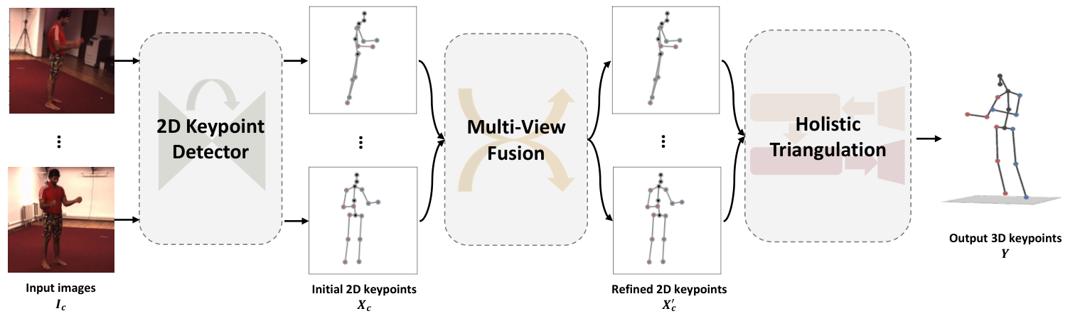
The overview of the proposed method is depicted in Fig. 1. There are three major modules: (1) 2D Keypoint Detector, to detect multi-view 2D joint locations respectively, where an off-the-shelf ResNet-152 backbone (Xiao et al. 2018) is directly applied. (2) Multi-View Fusion (MVF), to refine 2D poses considering the view consistency. (3) Holistic Triangulation (HT), to reconstruct the final 3D pose by closed-form optimization.
The input to the whole framework is a set of multi-view RGB images , whose index is the number of the synchronized cameras and . And the output is 3D pose , where and . Each image will be fed into the 2D detector to generate the initial 2D pose , where is the location of the joint in view . Then, the MVF module obtains the refined 2D poses from the initial ones by fusing all heatmaps corresponding to different views. After that, HT reconstructs the 3D pose from the refined 2D poses through optimization. Finally, a loss function, takes multi-view consistency and whole pose coherence into account, supervises the network when end-to-end training.
In this section, we first introduce HT, since the goal of our task is 3D pose. Then, the MVF is introduced as an assistance to refine the 2D results. Finally, the overall loss function of the end-to-end framework will be present.
3.1 Holistic Triangulation with Anatomy Constraints
LT is classic and elegant because of the closed-form solution, but is lack of joint-by-joint relation modeling. As depicted in Fig. 2(a), LT infers 3D position of each keypoint separately for times, and the keypoints are then concatenated to generate the 3D pose. To fix this issue, we propose Holistic Triangulation (HT), shown in Fig. 2(b), to reason the whole pose at once through reprojection and reconstruction term:
| (1) |
where is the Hadamard product. is the first three columns of and is the last column. is same as LT (refer to supplementary). We draw the idea from Algebraic Triangulation (AT) (Iskakov et al. 2019) to add the learnable confidence to mitigate the impact of 2D positions with low confidence.
However, owing to the blockwise linear independence in the reprojection term of Eq. 1, resulting vector of each block in has no difference from AT. To solve this problem, we introduce a reconstruction term .


Vanilla Reconstruction Term. The reconstruction term aims to enhance the blockwise linear dependence in and inject anatomy coherence to . PCA (Hotelling 1933), a simple but effective module is chosen to model the anatomy prior for two major reasons: (1) The PCA low-dimension latent space is capable to extract the correlations between different keypoints and factor out the generic pose global context. The generality of the pose context is guaranteed by the fact that training data contains various motions. And then we approach the estimated pose close to the PCA recovered pose from the latent space, to inject the pose prior. (2) The linear property of PCA will not change the closed-form solution superiority of HT, which will not hinder end-to-end training.
Note that the training set of PCA is root-relative, . And is the pelvis position which is estimated by LT. By adding a reconstruction term, the objective function is expressed as:
| (2) |
where is the recovered pose; is the feature extracting matrix of PCA encoder; is the mean pose of PCA training set; and is a learnable weight of reconstruction term. Because of the convexity of Eq.2, the 3D pose can be closed-form solved using Least-Square method (see supplementary for proof):
| (3) |
where .
| Method | shlder | elb | wri | hip | knee | ankle | root | belly | neck | nose | head | Avg. |
| CrossView (Qiu et al. 2019) | 95.6 | 95.0 | 93.7 | 96.6 | 95.5 | 92.8 | 96.7 | 96.4 | 96.5 | 96.4 | 96.2 | 95.9 |
| Epipolar (He et al. 2020) | 97.7 | 97.3 | 94.9 | 99.8 | 98.3 | 97.6 | 99.9 | 99.9 | 99.8 | 99.7 | 99.5 | 98.3 |
| ours-dot | 96.4 | 96.8 | 99.8 | 97.2 | 98.3 | 99.5 | 97.3 | 99.7 | 99.8 | 99.6 | 93.7 | 98.0 |
| ours-fcl | 97.8 | 97.5 | 99.8 | 97.7 | 98.7 | 99.6 | 97.8 | 99.7 | 99.8 | 99.8 | 95.4 | 98.5 |
| MPJPE (mm) | Dir. | Disc. | Eat | Greet | Phone | Photo | Pose | Purch. | Sit | SitD. | Smoke | Wait | WalkD. | Walk | WalkT. | Avg. |
| Canonical (Remelli et al. 2020) | 27.3 | 32.1 | 25.0 | 26.5 | 29.3 | 35.4 | 28.8 | 31.6 | 36.4 | 31.7 | 31.2 | 29.9 | 26.9 | 33.7 | 30.4 | 30.2 |
| CrossView-T. (Qiu et al. 2019) | 25.2 | 27.9 | 24.3 | 25.5 | 26.2 | 23.7 | 25.7 | 29.7 | 40.5 | 28.6 | 32.8 | 26.8 | 26.0 | 28.6 | 25.0 | 27.9 |
| Epipolar-T. (He et al. 2020) | 29.0 | 30.6 | 27.4 | 26.4 | 31.0 | 31.8 | 26.4 | 28.7 | 34.2 | 42.6 | 32.4 | 29.3 | 27.0 | 29.3 | 25.9 | 30.4 |
| Algebraic-T. (Iskakov et al. 2019) | 20.4 | 22.6 | 20.5 | 19.7 | 22.1 | 20.6 | 19.5 | 23.0 | 25.8 | 33.0 | 23.0 | 21.6 | 20.7 | 23.7 | 21.3 | 22.6 |
| ours-MVF | 20.1 | 21.5 | 20.0 | 18.7 | 21.3 | 20.3 | 18.4 | 21.9 | 24.3 | 30.6 | 22.1 | 20.4 | 19.6 | 23.4 | 20.2 | 21.6 |
| ours-HT | 19.4 | 21.5 | 20.0 | 18.7 | 21.6 | 20.9 | 18.2 | 21.5 | 24.8 | 31.7 | 21.7 | 20.2 | 18.9 | 23.2 | 19.6 | 21.6 |
| ours | 19.5 | 20.9 | 19.5 | 18.3 | 21.1 | 20.0 | 17.9 | 21.3 | 23.9 | 30.1 | 21.6 | 19.9 | 18.9 | 22.8 | 19.5 | 21.1 |
Skeletal Structure Feature Extraction Module. One inadequacy of the basic reconstruction term above is that the prior extracted is implicit. To address this, we transform the data from keypoint space to skeletal structure space, enhancing associations between joints and introducing explicit features.
To generate skeletal structure feature , KCS, a matrix multiplication algorithm to create vector between two selected points, is used to transform joints to joint-connected vectors by a mapping matrix . And is applied to transform back.
The feature of connected joint with hops is named as . As shown in Fig. 4, both keypoints and bone vectors can be compatible with and . Because longer distances will result in fewer extracted vectors with less information, only is defined. By fusing different features, the objective function can be adapted to:
| (4) |
where remaps the reconstructed error from feature space back to keypoint space in order to keep two terms in the same dimension. Replacing with and the solution is:
| (5) |
where .
3.2 Multi-View Fusion 2D Keypoint Refinement
The initial 2D keypoints achieved by 2D backbone detector are independent from each view. To enhance the cross view correlations, we introduce the MVF module. The pipeline of MVF is illustrated in Fig. 4. To make the keypoints in the reference view consistent with other views, the pseudo heatmaps corresponding to the same keypoints in other views are generated. Concretely, the pseudo heatmap is the product of matching heatmap and epipolar mask, and represents the probability source view keypoint localizing in the reference view. After that, the initial heatmap are fused with pseudo heatmaps through an aggregation layer which is a convolution kernel to product the refined fused heatmap.
Matching Layer. The idea of cost volume in stereo matching methods (Kendall et al. 2017; Xu and Zhang 2020) inspires us. The corresponding matching heatmaps , which indicates the matching degree of the keypoints in the source view and all pixels in the reference view, is generated. The pixel gets higher matching score as its features are better matched with . We also explore two types of matching strategy:
- 1.
inner dot:
- 2.
fully connected layer:
where represents the features generated by 2D backbone, is the sampled feature of via bilinear interpolation, means concatenation and is the learnable parameters.
Epipolar Layer. In stereo matching task, only the points in the horizontal direction will be compared because the given image pair are rectified. However, in matching layer, the is compared with all pixels in the reference view due to lack of rectification. The matching instability will be caused by the similar feature vectors of wrong pixels. To solve the problem, we generate the epipolar mask by the epipolar field (Ma et al. 2021) to limit the matching pixels locating near the epipolar line of . The epipolar field indicates the probability pixels in the reference view lies in the epipolar line of :
| (6) |
where are camera centers and is the soft factor to control the epipolar field margin. The field gets narrower as gets bigger, we choose to generate our epipolar mask by empirical results.
3.3 Loss
The overall loss function consists of four parts: (1) Mean Square Error (MSE) between estimated 3D pose and groundtruth, (2) reprojected error: L2 loss of reprojeted 2D pose and estimated 2D pose, (3) bone length loss: L1 loss of estimated bone vector and groundtruth and (4) joint angle loss of 3D poses:
| (7) |
where is the groundtruth of the pose; , and are set to 0.1, 0.01, 0.01 separately by empirical results. Based on the common , we subjoin the to enhance the multi-view consistency and to promote the anatomy coherence.
Joint Angle Loss. The multivariate GMM is used to model joint angle distribution , , and are azimuth and polar angle of joint in a local spherical coordinate system (Akhter and Black 2015) (details in suppl.). And the joint angles with low probability are penalized:
| (8) |
where is the number of selected joints; is probability border , the angle with the probability should be penalized. So transformation , coefficient are used to offset to to suit the variable domain of sigmoid.
4 Experiments
4.1 Datasets and Evaluate Metrics
Human3.6M Dataset. The Human3.6M (Ionescu et al. 2013) is one of the most universal 3D HPE dataset with 3.6 million annotations. The videos are acquired from 4 synchronized cameras in laboratory. We use Joint Detection Rate (JDR) to evaluate 2D pose, Mean Per Joint Position Error (MPJPE) to evaluate relative 3D pose and Percentage of Plausible Pose (PPP), elaborated in Sec. 4.2, to assess plausibility.
Total Capture Dataset. The Total Capture Dataset (Trumble et al. 2017) is a common dataset recorded by 8 cameras which are distributed over different pitch angles from top to bottom. The dataset contains various actions, including some challenging motions like crawling and yoga. Hence, cross-dataset experiments are executed on it to evaluate the generalization.
4.2 Plausible-Pose Evaluation Metric
Plausible-Pose Protocol. A plausible pose should meet two requirements: all bones have appropriate length and all joints are flexed in a limited range. A suitable bone length should be as near as possible to the groundtruth, and a reasonable joint angle is located in an occupancy matrix which indicates whether the angle pair appears in the training set:
| (9) |
where is bone length groundtruth and is bone length proportion threshold. The morphology technique is used to smooth the occupancy matrix , so that the continuous feasibility space can be covered even though the is discrete. Ultimately, a reasonable pose is:
| (10) |

Plausible-Pose Metric. To evaluate the plausibility performance statistically in testing dataset, a new metric PPP is defined as:
| (11) |
where is the number of testing samples, and the metric is divided according to the bone length threshold into PPP.
4.3 Comparison with State-of-The-Art Methods
We compare quantitative and qualitative performance with the state of the art using all views on Human3.6M, and conduct cross-dataset experiments on Total Capture.
Implementation Details. The low-dimension feature extraction matrix and mean pose of PCA are both generated by training set of Human3.6M and MPII-INF-3DHP. In order to avoid the influence of orientations diversity, the orientation normalization is applied in the training data. It should be clarified that hyperparameters and feature extraction strategies are determined by ablation study (supplementary): the feature , , are fused and the corresponding PCA reserved dimension are set to , , respectively; and coefficient of reconstruction term are learnable with initial value , , . We first train the MVF network with MSE loss of 2D keypoints on the training set of Human3.6M for 2 epochs with a batch size of 12. The learning rate is initially set to and decays every 25000 iterations by a factor of . After that, the whole network which combines three modules are trained for 4 epochs on the training set of Human3.6M with learning rate under the supervision of loss funtion described in Sec. 3.3. If not mentioned explicitly, the baseline is AT (Iskakov et al. 2019) method.
Quantitative Results on Human3.6M. We first evaluate the refined 2D results after MVF refinement module. Following convention, the threshold of JDR is set to the half of the head size. As shown in Table 1, MVF outperforms CrossView by at least regardless of the matching strategy. And fcl MVF also surpass Epipolar Transformer. The improvement demonstrates that the initial keypoint location can be leveraged to generate reliable pseudo heatmap with fewer calculations.
To evaluate the 3D pose estimation, we first compare precision performance with state-of-the-art methods whose input of 2D-3D step is only 2D keypoint locations. In addition to the whole framework, two networks are trained separately: (1) only MVF, uses MSE loss and reprojected loss to supervise, (2) only HT, supervised by MSE loss, bone length loss and joint angle loss. Both proposed modules achieves average MPJPE of , surpassing AT by (relative ). The improvement demonstrates that view consistency and anatomy coherence are both meaningful for pose estimation. As Table 2 shows, the method combined with two modules achieves the state-of-the-art results, with MPJPE, better than AT. And the performance is improved on almost all actions.
We also compare our approach with other methods whose input of 2D-3D reconstruction is heatmap or intermediate feature which contains more infromation than keypoint location. As shown in Table 3, our method achieves a balance of implementation complexity (calculated by thop11 1 https://github.com/Lyken17/pytorch-OpCounter), consuming time and accuracy performance. MVF-HT surpasses AT in both precision and plausibility with and , only at the cost of time consumption. Even though Volumetric Triangulation (VT) (Iskakov et al. 2019) surpasses us with MPJPE, the MVF-HT almost outperforms it by billion in the number of operations and in time costing. In 3D reconstruction procedure, VT utilizes 2D features as input and 3D CNN as inference network, which considers more information and is more complicate than ours. For the further work, we will explore the closed-form method that takes 2D features as input.
| Method | Input | Complexity | MPJPE (mm) | Time (ms) | PPP@0.2 () | |||
| feature | heatmap | keypoint | param | MACs | ||||
| CrossView-RPSM (Qiu et al. 2019) | ✓ | 570M | 424B | 26.2 | - | |||
| Epipolar-RPSM (He et al. 2020) | ✓ | 78M | 410B | 26.9 | - | |||
| Algebraic-T. (Iskakov et al. 2019) | ✓ | 79M | 418B | 22.6 | 75 | 79.36 | ||
| Volumetric-T.(Iskakov et al. 2019) | ✓ | 80M | 717B | 20.8 | 152 | - | ||
| ours | ✓ | 79M | 418B | 21.1 | 104 | 81.24 | ||
| MPJPE (mm) | Subject1,2,3 | Subject4,5 | Avg. | ||||
| W2 | FS3 | A3 | W2 | FS3 | A3 | ||
| IMUPVH*(Trumble et al. 2017) | 30 | 91 | 49 | 36 | 112 | 10 | 70 |
| AutoEnc*(Trumble et al. 2018) | 13 | 49 | 24 | 22 | 71 | 40 | 35 |
| CrossView*(Qiu et al. 2019) | 19 | 28 | 21 | 32 | 54 | 33 | 29 |
| GeoFuse*(Zhang et al. 2020) | 14 | 26 | 18 | 24 | 49 | 28 | 25 |
| baseline | 64 | 60 | 53 | 72 | 78 | 62 | 63 |
| ours | 45 | 49 | 45 | 52 | 64 | 57 | 51 |
| ours* | 13 | 24 | 17 | 23 | 41 | 29 | 23 |
| Matching Strategy | View |
| ||||
| dot | fcl | most-conf | all | |||
| 22.60 | ||||||
| ✓ | ✓ | 22.05 | ||||
| ✓ | ✓ | 21.88 | ||||
| ✓ | ✓ | 21.92 | ||||
| ✓ | ✓ | 21.61 | ||||
| Strategy | MPJPE (mm) | PPP (%) | ||
| PJ | BL | JA | ||
| 22.60 | 79.36 | |||
| ✓ | 22.12 | 79.37 | ||
| ✓ | 22.23 | 79.55 | ||
| ✓ | 22.40 | 79.43 | ||
| ✓ | ✓ | 22.10 | 79.68 | |
| ✓ | ✓ | ✓ | 21.89 | 79.70 |
| (views) | MPJPE (mm) | |||
| baseline | ours-HT | ours-MVF | ours | |
| 4 | 22.60 | 21.58 | 21.61 | 21.12 |
| 3 | 27.08 | 26.11 | - | - |
| 2 | 33.43 | 31.83 | 30.74 | 29.99 |
Qualitative Results on Human3.6M. To evaluate the multi-view consistency performance of MVF, the estimated, reprojected and groundtruth 2D keypoints are compared. The estimated 2D keypoint will be close to the reprojected keypoint from 3D result if the keypoint is consistent with other views. As illustrated in Fig. 5, the blue (reprojected) and green (estimated) points are generally closer after MVF refinement, especially for some self-occlusion. The improvement suggests that the MVF module can make views perceive others and provide assistant for some unseen view from other seen views.
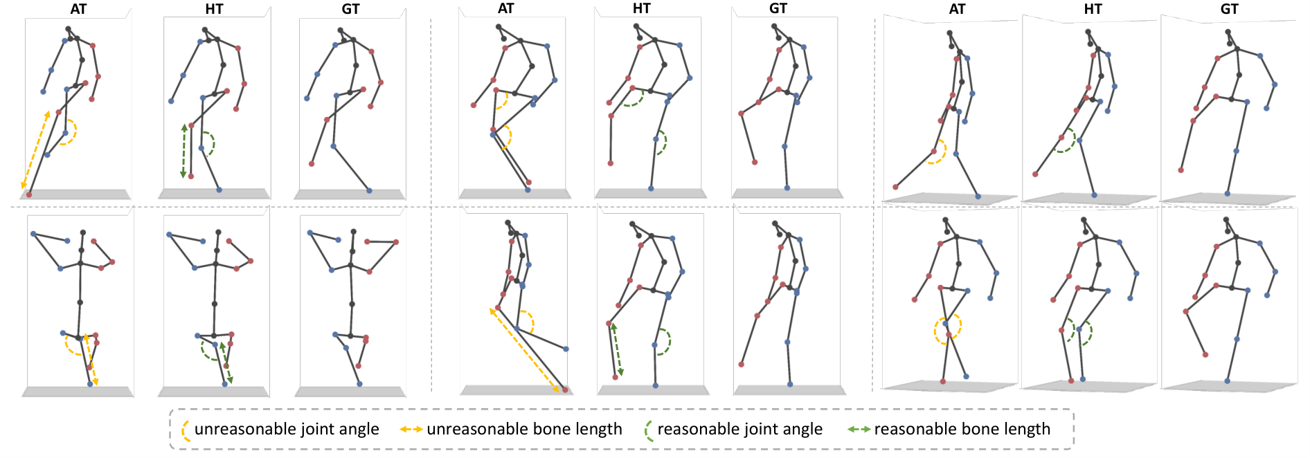
Furthermore, qualitative experiments are used to evaluate the ability to amend the implausible pose of HT approach. As illustrated in Fig. 6, the extracted anatomy prior can amend some unreasonable errors. It is particularly noteworthy that HT has the capability to correct the pose to have normal joint angles and bone lengths in such a tough situation.
Generalization to the Total Capture Dataset. To substantiate generalization of our model, we first conduct cross-dataset experiments on Total Capture, the testing model is only trained by Human3.6M training set. As shown in Table 4, our method surpasses baseline by (), which demonstrates the generalization of our method. Then we train our model with Total Capture training data under the same strategy clarified in Sec.4.3. Our method achieves MPJPE, which also exceeds GeoFuse (Zhang et al. 2020) by 8%. It is worth noting that, the PCA training set does not contain the Total Capture, which demonstrates that our anatomy coherence has the ability to deal with unseen gestures.
4.4 Ablation Study
All ablation studies are conducted on the Human3.6M. Both MPJPE and PPP metrics are used for evaluation.
MVF Module Evaluation. Beside the matching strategy, we also evaluate the number of views when fusing, there are two pipelines: (1) all view fusion, each view generates pseudo heatmap assist to other views, (2) most-conf fusion, only most-confident view is chosen to generate pseudo heatmap. The comparison is shown in Table 7, fully connected layer slightly outperforms the inner dot matching. And all view fusion performs better. We conjecture that since most initial results are reliable, as the number of fused views increases, more accurate auxiliary information is provided.
Effect of Loss. As shown in Table 7, PJ loss brings relative MPJPE improvement, which is more than bone length loss and joint angle loss. We suppose it is because that view consistency enhance correspondence of multi-view 2D keypoints. But the plausibility raises little with PJ loss. BL loss and JA loss bring more improvement in PPP. It demonstrates that the kinematic skeleton structure can boost the plausibility of pose. Finally we retrain the network which combines all loss function, and obtain the results whose MPJPE is and PPP is .
Effect of the Number of Views. Views are reduced from 4 to 2 during testing to explore influence of the number of views. As the number of views decreases, precision degrades. But MPJPE equals to when there are two views as shown in Table 7, which is still excellent. And compare ours with ours-HT or ours-MVF, the conclusion that both view consistency and anatomy coherence can improve pose estimation is proved.
Effect of Orientation Normalization. Whether and what the anatomy coherence PCA factors out still bother us. To observe it, we change each latent variable individually with a small step to generate the recovered 3D pose. The changes in 3D poses represents the physical meaning of the corresponding latent variable. Without orientation normalization, there are only 8 out of 25 latent variables describe joint correlations in motion, and the remaining 17 describe rotation invariant property. And the results have been improved after orientation normalization. The 25 variables all describe the joint-coupled motion. And the transformation of the recovered 3D poses demonstrate the capability of PCA to restrict joints correlation through motion.
5 Conclusion
We propose view consistency aware holistic triangulation to improve the performance of both precision and plausibility in 3D HPE. The key contribution is that the geometric correspondences of multi-view 2D keypoints are enhanced and anatomy coherence is injected to 2D-3D process. Meanwhile, a PPP metric is raised to evaluate the pose plausibility. Experiments not only exhibit that our approach outperforms state-of-the-art methods, but also demonstrate that the reconstruction term with extracted skeletal structure features can abstract the human anatomy prior.
References
- Akhter and Black (2015) Akhter, I., Black, M.J., 2015. Pose-conditioned joint angle limits for 3d human pose reconstruction, in: Proceedings of the IEEE conference on computer vision and pattern recognition, pp. 1446–1455.
- Bogo et al. (2016) Bogo, F., Kanazawa, A., Lassner, C., Gehler, P., Romero, J., Black, M.J., 2016. Keep it smpl: Automatic estimation of 3d human pose and shape from a single image, in: Computer Vision–ECCV 2016: 14th European Conference, Amsterdam, The Netherlands, October 11-14, 2016, Proceedings, Part V 14, Springer. pp. 561–578.
- Burenius et al. (2013) Burenius, M., Sullivan, J., Carlsson, S., 2013. 3d pictorial structures for multiple view articulated pose estimation, in: Proceedings of the IEEE conference on computer vision and pattern recognition, pp. 3618–3625.
- Cai et al. (2019) Cai, Y., Ge, L., Liu, J., Cai, J., Cham, T.J., Yuan, J., Thalmann, N.M., 2019. Exploiting spatial-temporal relationships for 3d pose estimation via graph convolutional networks, in: ICCV, pp. 2272–2281.
- Chen et al. (2019a) Chen, C.H., Tyagi, A., Agrawal, A., Drover, D., Mv, R., Stojanov, S., Rehg, J.M., 2019a. Unsupervised 3d pose estimation with geometric self-supervision, in: Proceedings of the IEEE/CVF Conference on Computer Vision and Pattern Recognition, pp. 5714–5724.
- Chen et al. (2019b) Chen, X., Lin, K.Y., Liu, W., Qian, C., Lin, L., 2019b. Weakly-supervised discovery of geometry-aware representation for 3d human pose estimation, in: Proceedings of the IEEE/CVF conference on computer vision and pattern recognition, pp. 10895–10904.
- Dong et al. (2019) Dong, J., Jiang, W., Huang, Q., Bao, H., Zhou, X., 2019. Fast and robust multi-person 3d pose estimation from multiple views, in: Proceedings of the IEEE/CVF conference on computer vision and pattern recognition, pp. 7792–7801.
- Gavrila and Davis (1996) Gavrila, D.M., Davis, L.S., 1996. 3-d model-based tracking of humans in action: a multi-view approach, in: Proceedings cvpr ieee computer society conference on computer vision and pattern recognition, IEEE. pp. 73–80.
- Guo et al. (2021) Guo, Y., Ma, L., Li, Z., Wang, X., Wang, F., 2021. Monocular 3d multi-person pose estimation via predicting factorized correction factors. Computer Vision and Image Understanding 213, 103278.
- Habibie et al. (2019) Habibie, I., Xu, W., Mehta, D., Pons-Moll, G., Theobalt, C., 2019. In the wild human pose estimation using explicit 2d features and intermediate 3d representations, in: Proceedings of the IEEE/CVF conference on computer vision and pattern recognition, pp. 10905–10914.
- Hartley and Zisserman (2003) Hartley, R., Zisserman, A., 2003. Multiple view geometry in computer vision. Cambridge university press.
- He et al. (2020) He, Y., Yan, R., Fragkiadaki, K., Yu, S.I., 2020. Epipolar transformers, in: Proceedings of the ieee/cvf conference on computer vision and pattern recognition, pp. 7779–7788.
- Hotelling (1933) Hotelling, H., 1933. Analysis of a complex of statistical variables into principal components. Journal of educational psychology 24, 417.
- Ionescu et al. (2013) Ionescu, C., Papava, D., Olaru, V., Sminchisescu, C., 2013. Human3. 6m: Large scale datasets and predictive methods for 3d human sensing in natural environments. IEEE transactions on pattern analysis and machine intelligence 36, 1325–1339.
- Iskakov et al. (2019) Iskakov, K., Burkov, E., Lempitsky, V., Malkov, Y., 2019. Learnable triangulation of human pose, in: Proceedings of the IEEE/CVF international conference on computer vision, pp. 7718–7727.
- Kadkhodamohammadi and Padoy (2021) Kadkhodamohammadi, A., Padoy, N., 2021. A generalizable approach for multi-view 3d human pose regression. Machine Vision and Applications 32, 6.
- Kendall et al. (2017) Kendall, A., Martirosyan, H., Dasgupta, S., Henry, P., Kennedy, R., Bachrach, A., Bry, A., 2017. End-to-end learning of geometry and context for deep stereo regression, in: Proceedings of the IEEE international conference on computer vision, pp. 66–75.
- Kocabas et al. (2019) Kocabas, M., Karagoz, S., Akbas, E., 2019. Self-supervised learning of 3d human pose using multi-view geometry, in: Proceedings of the IEEE/CVF conference on computer vision and pattern recognition, pp. 1077–1086.
- Liu et al. (2020) Liu, K., Zou, Z., Tang, W., 2020. Learning global pose features in graph convolutional networks for 3d human pose estimation, in: Proceedings of the Asian Conference on Computer Vision.
- Ma et al. (2021) Ma, H., Chen, L., Kong, D., Wang, Z., Liu, X., Tang, H., Yan, X., Xie, Y., Lin, S.Y., Xie, X., 2021. Transfusion: Cross-view fusion with transformer for 3d human pose estimation. arXiv preprint arXiv:2110.09554 .
- Malleson et al. (2020) Malleson, C., Collomosse, J., Hilton, A., 2020. Real-time multi-person motion capture from multi-view video and imus. International Journal of Computer Vision 128, 1594–1611.
- Martinez et al. (2017) Martinez, J., Hossain, R., Romero, J., Little, J.J., 2017. A simple yet effective baseline for 3d human pose estimation, in: Proceedings of the IEEE international conference on computer vision, pp. 2640–2649.
- Pavlakos et al. (2017a) Pavlakos, G., Zhou, X., Derpanis, K.G., Daniilidis, K., 2017a. Coarse-to-fine volumetric prediction for single-image 3d human pose, in: Proceedings of the IEEE conference on computer vision and pattern recognition, pp. 7025–7034.
- Pavlakos et al. (2017b) Pavlakos, G., Zhou, X., Derpanis, K.G., Daniilidis, K., 2017b. Harvesting multiple views for marker-less 3d human pose annotations, in: Proceedings of the IEEE conference on computer vision and pattern recognition, pp. 6988–6997.
- Qiu et al. (2019) Qiu, H., Wang, C., Wang, J., Wang, N., Zeng, W., 2019. Cross view fusion for 3d human pose estimation, in: Proceedings of the IEEE/CVF international conference on computer vision, pp. 4342–4351.
- Remelli et al. (2020) Remelli, E., Han, S., Honari, S., Fua, P., Wang, R., 2020. Lightweight multi-view 3d pose estimation through camera-disentangled representation, in: Proceedings of the IEEE/CVF conference on computer vision and pattern recognition, pp. 6040–6049.
- Tian et al. (2021) Tian, L., Wang, P., Liang, G., Shen, C., 2021. An adversarial human pose estimation network injected with graph structure. Pattern Recognition 115, 107863.
- Trumble et al. (2018) Trumble, M., Gilbert, A., Hilton, A., Collomosse, J., 2018. Deep autoencoder for combined human pose estimation and body model upscaling, in: Proceedings of the European Conference on Computer Vision (ECCV), pp. 784–800.
- Trumble et al. (2017) Trumble, M., Gilbert, A., Malleson, C., Hilton, A., Collomosse, J., 2017. Total capture: 3d human pose estimation fusing video and inertial sensors, in: Proceedings of 28th British Machine Vision Conference, pp. 1–13.
- Tu et al. (2020) Tu, H., Wang, C., Zeng, W., 2020. Voxelpose: Towards multi-camera 3d human pose estimation in wild environment, in: Computer Vision–ECCV 2020: 16th European Conference, Glasgow, UK, August 23–28, 2020, Proceedings, Part I 16, Springer. pp. 197–212.
- Wandt et al. (2018) Wandt, B., Ackermann, H., Rosenhahn, B., 2018. A kinematic chain space for monocular motion capture, in: Proceedings of the European Conference on Computer Vision (ECCV) Workshops, pp. 0–0.
- Wandt and Rosenhahn (2019) Wandt, B., Rosenhahn, B., 2019. Repnet: Weakly supervised training of an adversarial reprojection network for 3d human pose estimation, in: Proceedings of the IEEE/CVF conference on computer vision and pattern recognition, pp. 7782–7791.
- Wang et al. (2021) Wang, J., Tan, S., Zhen, X., Xu, S., Zheng, F., He, Z., Shao, L., 2021. Deep 3d human pose estimation: A review. Computer Vision and Image Understanding 210, 103225.
- Xiao et al. (2018) Xiao, B., Wu, H., Wei, Y., 2018. Simple baselines for human pose estimation and tracking, in: Proceedings of the European conference on computer vision (ECCV), pp. 466–481.
- Xu and Zhang (2020) Xu, H., Zhang, J., 2020. Aanet: Adaptive aggregation network for efficient stereo matching, in: Proceedings of the IEEE/CVF Conference on Computer Vision and Pattern Recognition, pp. 1959–1968.
- Xu and Takano (2021) Xu, T., Takano, W., 2021. Graph stacked hourglass networks for 3d human pose estimation, in: Proceedings of the IEEE/CVF conference on computer vision and pattern recognition, pp. 16105–16114.
- Yang et al. (2022) Yang, J., Ma, Y., Zuo, X., Wang, S., Gong, M., Cheng, L., 2022. 3d pose estimation and future motion prediction from 2d images. Pattern Recognition 124, 108439.
- Zhang et al. (2020) Zhang, Z., Wang, C., Qin, W., Zeng, W., 2020. Fusing wearable imus with multi-view images for human pose estimation: A geometric approach, in: Proceedings of the IEEE/CVF Conference on Computer Vision and Pattern Recognition, pp. 2200–2209.
- Zhao et al. (2019) Zhao, L., Peng, X., Tian, Y., Kapadia, M., Metaxas, D.N., 2019. Semantic graph convolutional networks for 3d human pose regression, in: Proceedings of the IEEE/CVF conference on computer vision and pattern recognition, pp. 3425–3435.
- Zhou et al. (2016) Zhou, X., Zhu, M., Leonardos, S., Derpanis, K.G., Daniilidis, K., 2016. Sparseness meets deepness: 3d human pose estimation from monocular video, in: Proceedings of the IEEE conference on computer vision and pattern recognition, pp. 4966–4975.
Supplementary Materials
View Consistency Aware Holistic Triangulation for 3D Human Pose Estimation
1 2D Backbone Structure
The 2D backbone consists of ResNet-152 and three deconvolutional layers to produce the immediate features, followed by a convolutional kernel to generate 2D heatmaps with output channels. Where , is the number of keypoints, and is the index of view. 2D positions are calculated by soft-argmax, a differentiable approach which makes end-to-end training of 3D estimator possible. Soft-argmax treats the 2D keypoints as the centroid of heatmap , and the weight of each pixel is produced by softmax in heatmap:
where are width and height of the heatmap respectively, and is the location of the pixel in heatmap.
| Dimension | 51 | 35 | 30 | 25 | 20 | 15 | 10 |
| MPJPE- (mm) | 22.60 | 22.10 | 22.04 | 22.04 | 22.06 | 22.08 | 22.11 |
| PPP@0.2 (%) | 79.36 | 79.90 | 79.91 | 80.97 | 80.14 | 80.19 | 80.33 |
| Coefficient | 1 | 2 | 3 | 4 | 5 | 6 | 7 | 8 | 9 | 10 |
| MPJPE (mm) | 22.11 | 22.09 | 22.07 | 22.06 | 22.05 | 22.04 | 22.04 | 22.04 | 22.05 | 22.06 |
| PPP@0.2 (%) | 79.68 | 79.68 | 80.19 | 80.55 | 80.60 | 80.55 | 80.74 | 80.97 | 81.02 | 80.74 |
| Coefficient | 1 | 2 | 3 | 4 | 5 | 6 | 7 | 8 | 9 | 10 |
| MPJPE-re (mm) | 22.03 | 21.94 | 21.88 | 21.86 | 21.86 | 21.90 | 21.96 | 22.04 | 22.15 | 22.27 |
| PRP@0.2 (%) | 79.55 | 80.01 | 80.37 | 80.92 | 80.65 | 80.92 | 80.92 | 80.88 | 81.11 | 81.20 |
| Coefficient | 1 | 2 | 3 | 4 | 5 | 6 | 7 | 8 | 9 | 10 |
| MPJPE-re (mm) | 22.06 | 21.98 | 21.94 | 21.91 | 21.91 | 21.92 | 21.95 | 21.99 | 22.05 | 22.11 |
| PRP@0.2 (%) | 79.87 | 80.15 | 80.56 | 80.79 | 80.65 | 80.33 | 80.55 | 81.02 | 81.24 | 81.15 |
2 Linear Triangulation Theory
The homogeneous 2D and 3D keypoint can be expressed as , . The projected 2D keypoint from in the view is . To make the estimated and projected same, the target function can be written as:
and then:
where is the row of , so:
Finally, the target function can be expressed as , where
Change the 3D keypoint to inhomogeneous expression , the target function can be rewritten like:
where is the first three columns of and is the last column.
3 The Closed-Form Solution Proof
The objective function of Holistic Triangulation with anatomy constraints is:
where is the recovered pose; is the feature extracting matrix of PCA encoder; is the mean pose of PCA training set; ; and is a learnable weight of reconstruction term. Then objective function can be rewritten as:
Because of the property preserving convexity that nonnegative weighted sums and composition with an affine mapping have, the function is still convex. So, using Least-Square method to solve it, the closed form answer can be expressed as:
So the answer can be simplified to:
where .
4 KCS Details
The original KCS is a algorithm to create a vector between two defined joints using matrix multiplication. The target vector from to can be calculated as:
where and is the matrix of all 3D keypoints. To compatible with our 3D keypoints expression , the KCS can be rewritten as:
where is the matrix which maps the keypoint location vector to bone vector ; is the matrix maps back to ; and
which can transform two keypoints with index to the connected bone vector by .


5 Loss Detail
Reprojected Loss. The reprojected loss is expressed as the sum of the errors between reprojected keypoints from and refined keypoints :
Bone Length Loss. L1 norm is utilized to measure distance of bone length between the solved pose and the annotation:
where represents the bone length and is the groundtruth.
Joint Angle Distribution The angle of the joint is defined as the angle between two bones connected to this joint. To calculate it, we convert the global coordinate to a local spherical coordinate system and get the azimuth and polar angle .
The distributions of all selected angles almost fit the Gaussian Mixture Module (GMM), which can be illustrated as in Fig. 2. After expanding into 3D space, the distribution can be observed more intuitively in Fig. 2. Here, we select nine joints angles: right-shoulder, right-elbow, left-shoulder, left-elbow, right-hip, right-knee, left-hip, left-knee, and spine. The multivariate GMM is used to model the distribution of joint angle in this way:
where and are parameters and weights of the module; the angle of the joint is represent by . Trigonometric functions are used to address the discontinuity stepping from to .
6 HT Module Design
It should be mentioned that HT is only used as a post-processing step, replacing the baseline triangulation, to determine the hyperparameters.
First, we compare different choices of low-dimension preserved by PCA. As the dimension decreases, less variance is kept, which means lower precision but higher abstraction. As shown in Table 1, we change from to with stride , which corresponds to preserving variance from to . As decreases, both precision MPJPE and PPP get improved, and peaks at ( variances) where a balance is struck in prior extraction and precision preservation. Compared with baseline, the improvement demonstrates the importance of PCA reconstruction term, implying that the pose global context is extracted.
Then, different coefficients of vanilla reconstruction term ( feature, others can be found in supplementary) are evaluated. The magnitude of is set to to make the reprojection term and reconstruction term approximate . is our final choice due to its balance between MPJPE and PPP, as shown in Table 2. The increase of does not bring much improvement to MPJPE but improves more on PPP. For one thing, the coefficient variation has little effect on the accuracy when two terms are of the same magnitude. For another, the observation that average accuracy does not equal to reasonability can be verified. We compare performance on different threshold of PPP which represent different tolerance for implausible pose. As illustrated in Fig. 3, reconstruction term almost yields more than growth compared with baseline regardless of different and . It demonstrates that our anatomy term can improve the poses with different degrees of implausibility, especially when the degree is low.
We finally use training set to extract different vectors, and then generate corresponding PCA extraction matrices to compare different feature extraction strategy. As shown in Table 5, which conforms to the human skeleton performs slightly better, and precision in also surpasses , which can justify the effect of skeleton structural feature. Then, we fuse them, the strategy which combines three types yields improvement by (relative ) in MPJPE and (relative ) in PPP. It should be noted that, adding different features does not bring corresponding increase as same as the individual condition. We hypothesize that all features are extracted from one data source, so stacking them does not yield much information gain.
| Strategy | MPJPE (mm) | PPP () | ||
| hop=0 | hop=1 | hop=2 | ||
| 22.60 | 79.36 | |||
| ✓ | 22.04 | 80.97 | ||
| ✓ | 21.86 | 80.92 | ||
| ✓ | 21.91 | 80.79 | ||
| ✓ | ✓ | 21.83 | 80.97 | |
| ✓ | ✓ | ✓ | 21.78 | 81.24 |