LSFD for Rician-Faded Cell-Free mMIMO Systems With Channel Aging and Hardware Impairments
Abstract
We study the impact of channel aging on the uplink of a cell-free massive multiple-input multiple-output system with hardware impairments. We consider a dynamic analog-to-digital converter architecture at the access points (APs), and low-resolution digital-to-analog converters at the user equipments (UEs). We derive a closed-form spectral efficiency expression by considering i) practical spatially-correlated Rician channels; ii) hardware impairments at the APs and the UEs; iii) channel aging; and iv) large-scale fading decoding (LSFD). We show that LSFD can effectively mitigate the detrimental effects of i) channel aging for both low and high UE velocities; and ii) inter-user interference for low-velocity UEs but not for high-velocity UEs.
I Introduction
Cell-free (CF) massive multiple-input multiple output (mMIMO) is being investigated as a key technology for beyond fifth-generation wireless systems. This is because it can provide a uniformly high spectral efficiency (SE) in its entire coverage area [1]. A CF mMIMO system deploys a large number of access points (APs) [2], and avoids inter-cell interference via cooperation between APs, which are inter-connected using a central processing unit (CPU) [1, 2].
A CF mMIMO system, where APs and user equipments (UEs) are designed using high-quality radio frequency (RF) transceivers and high-resolution analog-to-digital converters (ADCs)/digital-to-analog converters (DACs), have a high implementation cost and energy consumption [2, 3, 4]. A CF mMIMO deployment is attractive when APs and UEs are designed using inexpensive RF transceivers and low-resolution ADC/DACs [1, 2]. To reduce the SE loss due to low-resolution ADC/DACs, the authors in [3, 4] considered a mixed-ADC architecture, wherein one fraction of AP antennas have a high-resolution ADCs, while the other has low-resolution. Zhang et. al in [3] and [4] investigated the SE of a CF mMIMO system with mixed-ADC architecture at the APs by considering spatially-uncorrelated Rayleigh and Rician-fading channels respectively, and showed its superiority over the low-resolution counterpart. The current work generalizes the mixed-ADC architecture in [4, 3], by considering a dynamic ADC architecture, wherein the resolution of ADC connected to each antenna can be varied from to maximum bits. This is in unlike [4, 3], wherein each AP antenna can either have a low or a high-resolution.
To further reduce the cost and energy consumption of CF mMIMO systems, the authors in [5, 6] assumed that the APs and UEs additionally employ low-cost RF transceivers. The low-cost RF transceivers, however, experience power amplifier non-linearities and phase noise, which degrade the benefits accrued from CF mMIMO technology [5, 6]. Masoumi et. al in [5] derived the uplink SE of a hardware-impaired uncorrelated Rayleigh-faded CF mMIMO system with limited-capacity fronthaul link between each AP and CPU. Tentu et. al in [6] investigated the SE of a spatially-correlated Rician-faded CF mMIMO system with low cost RF transceiver.
The aforementioned works analyzed the impact of low and mixed resolution ADCs and low-cost RF chains for Rayleigh-faded channels, except [4, 6] which considered Rician-faded channels. Rayleigh fading may not accurately characterize the propagation environment, as the UE-AP channel may contain line-of-sight (LoS) path due to its macro-diversity [7, 8]. Such a channel has a Rician probability distribution function (pdf). The phase of LoS path, which accounts for the phase-shift due to UEs mobility, is modeled as a uniformly distributed random variable [8]. The authors in [7, 6] did not consider phase-shifts in the LoS component while modeling the Rician channel. Jin et. al in [7] derived a closed-form SE expression for spatially-correlated Rician-faded CF mMIMO system by assuming perfect knowledge of phase-shifts. In practice, phase-shifts are hard to estimate [8]. The authors in [8] investigated the uplink and downlink SE of a uncorrelated Rician-faded CF mMIMO system by assuming unknown phase-shift, but with ideal hardware at the APs and UEs.
The UEs to AP channels are further subjected to time variations due to UE mobility, a phenomenon known as channel aging [9, 10]. Chopra et. al in [9] showed that the impact of channel aging is higher for a CF mMIMO than its counterpart. Zheng et. al in [10] analyzed the effect of channel aging in a CF mMIMO system for correlated Rayleigh fading channels. The authors in [9, 10], however, assumed cellular/CF mMIMO systems with ideal hardware. The current work analyzes the SE of a spatially-correlated Rician-faded CF mMIMO system with random LoS phase-shifts, low-cost RF chains, and dynamic-ADC/DAC architecture.
It is practically difficult, due to the limited coherence block, to assign orthogonal pilots to each user. This pilot sharing across users leads to pilot contamination. A two-layer large-scale fading decoding (LSFD) is proposed to combat it [11, 12].
Trinh et. al in [11] showed that in Rayleigh-faded cellular mMIMO systems LSFD significantly reduces the impact of pilot contamination, which conserably improves the SE. Ozlem et. al in [12] maximized the minimum SE in a wireless-powered Rician-faded CF mMIMO system with LSFD. The authors in [11, 12], however assumed ideal hardware.
The existing CF mMIMO works, to the best of our knowledge have not even investigated the performance of a hardware-impaired CF mMIMO system with spatially-correlated Rician-fading channel and aging.
We next summarize the main contributions of the current work, which address these gaps:
We consider a CF mMIMO system with spatially-correlated Rician-faded channels with aging, and investigate the impact of dynamic-ADC architecture and low-cost hardware-impaired RF chains. We also consider a two-layer LSFD and derive a closed-form SE expression by addressing the derivation difficulties caused by the combined modelling of channel aging, LSFD, RF impairments, dynamic ADC/DAC architecture and spatially-correlated Rician channels.
We show that LSFD, even in presence of hardware impairments and channel aging, provides high SE gain over single layer decoding. Further, LSFD effectively mitigates the degradation due to channel aging for both low and high UE
velocities. It can, however, mitigate inter-user interference (IUI) only for low-velocity UEs, and not for high-velocity UEs.
II System Model
We consider the uplink of a CF mMIMO system with multi-antenna APs, each equipped with antennas, and single-antenna UEs. We assume, similar to [12, 2], that the APs are randomly distributed over a large geographical area, and are connected to a CPU via high-speed fronthaul links. To reduce the system hardware cost and power consumption, both APs and UEs are equipped with cost-effective RF chains. Further, the APs have a dynamic-resolution ADC architecture, wherein each AP antenna can be connected to a different resolution ADC. The UEs are designed using low-resolution DACs. This is unlike [2, 4, 3] , which model all the ADCs as either low- or mixed-resolution.
We also assume that the CF mMIMO system, due to UEs mobility, observes channel aging. To investigate its impact, we consider a resource block, each of length time instants [10]. The channel remains constant for a time instant, and varies across time instants in a correlated manner. This temporal correlation is modeled later using Jake’s model [9]. We also assume that each resource block is divided into an uplink training and data transmission interval of lengths and time instants, respectively. We next discuss the UE-AP uplink channel, and then the uplink training and data transmission protocols.
Channel model: The channel from the th UE to the th AP at the th time instant is denoted as . Due to dense AP deployment, contains both LoS and non-LoS paths, and, therefore, has a Rician pdf [8] i.e.,
| (1) |
Here and . The term is the Rician factor, and is the large-scale fading coefficient. The LoS term is modeled as , where is the angle of arrival between the th AP and the th UE. The term, , with pdf , models the small-scale fading, and characterizes the spatial correlation matrix of the NLoS path. The phase-shift at the th instant is uniformly distributed between .
The long-term channel statistics i.e., , and , remain constant over a resource block and, similar to the existing literature [8, 12], are perfectly known at the AP. The LoS phase-shift , similar to small-scale fading component, varies at each time instant [8, 12]. Most of the Rican CF works e.g., [7, 6], assume a LoS path with static phase, and thus ignored its effect. A slight change in UEs position and hardware impairments can radically change the phase. It is crucial to consider this phase-shift to realistically model the Rician channel [8, 12]. We, similar to [8, 12], model the channel by assuming that the LoS phase varies as frequently as small-scale fading, and consequently the AP is unaware of it. As an AP does not have prior knowledge of , it estimates the channel , without its knowledge.
The UEs mobility causes the AP-UE channel in a resource block to vary across the time instants, which causes channel aging [10]. We model the channel at the th time instant, as a combination of its initial channel , and innovation component as follows [10]:
| (2) |
Here is the temporal correlation coefficient, which based on the Jake’s model [10], is given as . The term is the zeroth-order Bessel function of the first kind, and is the sampling time. The term is the Doppler spread, with , and being the user velocity, carrier frequency and the velocity of light, respectively. The innovation component is independent of the channel , and has a pdf [10].
Uplink training:
Recall that the uplink training phase consists of time instants. The th UE, similar to [10], transmits its pilot signal at the time instant . Here .
We assume that the uplink training duration . The number of UEs transmitting pilot at a particular time instant is more than one, which causes pilot contamination [8]. The set of UEs that transmit pilots at the time instant is denoted as . The th UE feeds its pilot signal to the low-resolution DAC, which distorts it. This distortion is commonly analyzed using Bussgang model [13]. The distorted DAC output, based on the Bussgang model, is:
Here is the DAC distortion factor and is the zero-mean DAC quantization noise, which is uncorrelated with the input pilot signal [8]. Its variance is given as . The th UE DAC output signal is then fed to its low-cost hardware-impaired RF chain whose output, based on the error vector magnitude (EVM) model, adds a distortion term to the transmit signal [14]. The effective uplink pilot signal is, therefore, given as . Here is the distortion term, which is independent of the input signal, and has a pdf [14]. The term models the UE transmit EVM [14].
| (6) |
The pilot signals received at the antennas of the th AP at the time instant is
| (3) |
To reduce the system cost, APs are designed using low-cost hardware-impaired RF chains and a dynamic-ADC architecture, which enables us to vary the resolution of each ADC from to maximum of bits. The th AP feeds the pilots signal received at its antenna to the low-cost RF chains, whose distorted output, based on the EVM model, is [6]:
| (4) |
The term , with pdf , models the hardware distortion due to the low-cost RF chains. The term is the AP receiver EVM and . The vector , with pdf , is the AWGN at the th AP. The RF chain output is then fed to the dynamic resolution ADCs, which distorts it by adding quantization noise. The distorted ADCs output, based on the Bussgang model [13], is given as
| (5) |
The matrix , where is the ADC distortion factor [13]. The zero-mean additive ADC quantization noise is uncorrelated with . Its covariance is with [13]. The existing CF mMIMO literature [2, 4, 3], has not investigated the dynamic resolution ADC architecture with different diagonal elements of i.e., for . It significantly complicates the SE analysis and derivation, when compared with [2, 4, 3], which considers either low- or mixed-ADC architecture at the APs. Our architecture is generic, and reduces to its low-resolution and mixed-resolution counterparts with and , respectively.
We next substitute expressions of and from (3) and (4) in (5), and re-express as
Here . Recall that the channel between the two different time instants ages, and is consequently correlated. The received signal can be exploited while estimating channel at any other time instant also. The channel estimate quality will, however, deteriorate with increasing time difference between the pilot transmission () and the considered channel realization (). We, therefore, without loss of generality, estimate the channel at the time instant , and use these estimates to obtain channels at all other time instants . To obtain the channel at the th time instant, the received pilot signal is expressed in terms of the channel at the time instant , using (2) as given in (6) at the top of the page. Here and . Using , the channel is estimated in the following theorem. The proof, due to page constraints, is provided in [15].
Theorem 1.
For a hardware-impaired CF mMIMO system with spatially-correlated Rician fading and phase-shifts, the linear minimum mean square error (LMMSE) estimate of is:
| (7) |
and .
| (11) |
| , with . | |
The LMMSE estimation error has zero mean, and covariance matrix . The estimate is uncorrelated with the error . The channel estimator derived in [10], by assuming Rayleigh fading and ideal RF chains and ADC/DAC, cannot be used herein. This is due to the hardware-impaired RF chains and dynamic-resolution ADC/DAC architecture, we need to compute , which [10] need not. Uplink Transmission: Let , with , be the information symbol which the th UE wants to transmit at the th time instant. The symbol , after scaling with power control coefficient , is fed to the low-resolution DAC. Its distorted output, based on the Bussgang model [13], is given as . Here is the DAC distortion factor and is the DAC quantization noise [13]. It is uncorrelated with the information signal , has a zero mean and variance . The DAC output is fed to the low-cost hardware-impaired RF chain, whose distorted output, based on the EVM model, is [14]:
| (8) |
The term is the transmit RF hardware impairment of the th UE, and has pdf , with being the transmit EVM [5]. The th AP receives the following sum signal at its antenna: . The AP feeds this receive signal to its hardware-impaired RF chains, which distorts it as[5]:
| (9) |
Here , with pdf , is the receiver hardware distortion, and . The term with pdf is the th AP AWGN. The RF chain output is then fed to the dynamic-resolution ADCs, whose noisy output, based on the Bussgang model [13], is given as:
| (10) |
The matrix , with being the ADC distortion factor for the th antenna. The vector is the quantization noise which is uncorrelated with the input signal . It has a zero mean and covariance where and [13].
Two-layer decoding: The CF system considered herein employs two-layer decoding to mitigate the IUI. In the first-stage, each AP combines its received signal by using the local channel estimates, which mitigates a part of the IUI. To mitigate the residual IUI, all APs send their locally-combined received signal to the CPU, which performs the second-layer LSFD. The CPU computes the LSFD weights based on the large-scale fading coefficients, which it can easily compute at they remain constant for s of coherence intervals [12].
The th AP first uses channel estimate to combine the distorted received signal as
.
It sends its combined signal to the CPU which performs second-layer LSFD as . Here is the complex LSFD coefficient of the th AP and the th UE link. This reduces the IUI by weighing the received signals from all APs. We now re-express the signal as given in (II) at
the top the page and use this to calculate the closed-form SE.
III Spectral efficiency Analysis
We derive the closed-form SE expression by using the use-and-then-forget UaTF technique [10, 14]. It expresses the LSFD-combined signal at the AP in (II), as follows:
The effective noise term consists of all the terms given in (II), except the first term and the beamforming uncertainty term . The first term in , which is used for signal detection, requires only long channel information [10]. Using central limit theorem, the effective noise can be approximated as worst-case Gaussian [14]. A lower bound to calculate the SE of a hardware-impaired CF mMIMO system with spatially-correlated Rician fading and channel aging for a given LSFD weights as [14]: , where
| (12) |



The term is the desired signal strength, is the beamforming uncertainty strength, is the interference strength, is the UE DAC impairment strength, is the UE RF impairment strength, is the AP RF impairment strength, is the AP ADC impairment noise and is the AWGN strength. These terms are defined as in Table I. Here , . These expectations next need to be computed to derive the closed-form SE expression. The presence of i) channel aging; ii) spatially correlated Rician channel with phase-shifts; iii) RF impairments and dynamic ADC architecture at the APs; iv) RF impairments and low-resolution DAC at the UEs; and v) LSFD, significantly complicates their computation, when compared with existing CF channel aging literature [10], which considered Rayleigh fading with ideal hardware. Their simplification requires novel mathematical results, and are not a straightforward extension of [10]. We next derive the lower bound in the following theorem.
Theorem 2.
The closed-form SE expression, for an arbitrary number of antennas with channel aging, RF and ADC/DAC impairments both at the APs and the UEs, LSFD and spatially-correlated Rician channel with phase-shifts, is given as
| (13) |
Here
.
with ,
, . The matrix diagonal and off-diagonal elements are given as and respectively.
The terms , , are given in Appendix A.
We see from (13) that the SINR expression is a generalized Rayleigh quotient with respect to . The optimal LSFD coefficients are given as [14, Lemma B.10].
Corollary 1.
We can simplify the sum-SE expression in (13) for ideal hardware, and show that it matches with the existing work [1, 10]. This not only validates our results theoretically but also shows that the current work subsumes the existing work [1, 10]. By setting i) Rician factor ; ii) ; and iii) ideal RF hardware and high ADC/DAC resolution, the expression is
| (14) | ||||
This above expression matches with [10, Eq. (21)]. Also, with , , , and , the expression in (14) matches with [1, Eq. ].
| For , | . |
| For , | |
| For , ; For , . | |
| ; For , , . | |
| , , . | |
IV Simulation Results
We now numerically validate the derived closed-from SE in (13) and investigate the i) effect of channel aging; ii) RF and ADC/DAC impairments; iii) Rician phase-shifts; and iv) LSFD. We consider a simulation setup where APs and UEs are randomly and uniformly distributed within an area of [1].
We use the local-scattering model from [14] to model the correlation matrix . We set the noise variances dBm, APs, UEs, antennas per AP, Km/hr and the pilot power dBm [14]. We model the Rician factor and the large-scale fading coefficients as in [8, Eq. (84)].
Validation of closed-form SE:
We first validate in Fig. 1(a) the derived closed-form SE expression in (13) by comparing it with its simulated counterpart in (12).
For this study, we consider following RF impairment and ADC/DAC combinations: i) ideal RF with , ADC/DAC; ii) , ideal ADC/DAC; iii) , dynamic ADC resolution; iv) ideal RF, -bit ADC/DAC resolution.
We see that for different combinations of RF and ADC/DAC impairments, the derived closed-form SE exactly matches with its numerical counterpart. This validates the derived closed form SE expression, which can thus be used for a realistic evaluation of hardware-impaired CF channel aging system.
Phase-aware and phase-unaware estimator performance:
We now study in Fig. 1(b) the effects of phase-aware and phase-unaware MMSE channel estimator on the SE with two-layer LSFD and single-layer decoding (SLD) by varying the UE velocity . The SLD can be obtained by considering in (13).
We first see that LSFD provide much higher SE than SLD. We also see that the phase-aware estimator has a higher SE than the phase-unaware estimator. This is because the phase knowledge helps in suppressing the interference [8]. Further, the SE gap between the two estimators reduces with increase in velocity. The, consequent, faster channel aging increases the correlation factor , which increases the interference due to channel aging in (12). This mitigates the gain of phase-aware channel estimator. We also see that for both LSFD and SLD, the SE gap between the phase-aware and phase-unaware estimator increases with non-ideal hardware.
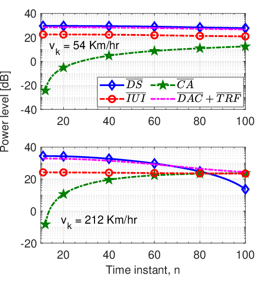
Effect of channel aging: We now numerically study in Fig. 1(c) and Fig. 1(d) the behavior of desired signal power, channel aging power, IUI power, and UE RF and DAC distortion power (labelled as , , and , respectively), for LSFD and SLD schemes. We assume that UEs have a velocity of Km/hr, and the remaining UEs have Km/hr. From Fig. 1(c), we observe the following:
- •
For high-velocity UEs, the and powers reduce with time (see the bottom subplot). This is because both these powers are functions of the temporal correlation coefficient , whose value, for a high UE velocity, reduces greatly with time. For low-velocity UEs, as shown in the top subplot, these powers are almost time-invariant.
- •
For high-velocity UEs and , we see that reduces monotonically, while power first tapers out, and then floors to a constant value. This is because the power decreases as , which decreases monotonically with . The transmit RF + DAC impairments reduce as , with being a constant. For , the constant term dominates the reduction due to , which makes the impairment power floor to a constant value.
We next compare Fig. 1(c) with Fig. 1(d), which plots the above power values for SLD. We see that for low-velocity UEs, LSFD has a much lower , and power than SLD. This is because the channels of low-velocity UEs do not significantly age, and consequently their channel estimates quality do not deteriorate. The LSFD can thus better suppress the IUI. For high-velocity UEs, LSFD yields much lower values than SLD, while both LSFD and SLD yield similar values. This implies that LSFD can mitigate the effect of channel aging for high-velocity UEs, but not IUI. This study shows that LSFD can mitigate i) the effect of channel aging for low/high UE velocities; and ii) IUI for low-velocity UEs.
V Conclusion
We derived and validated the closed-form SE expression for a hardware-impaired spatially-correlated Rician-faded CF mMIMO system with channel aging and LSFD. We numerically showed that the SE gap between the phase-aware and phase-unaware estimators reduces with increased UE velocity, and increases with hardware impairments. We also showed that the LSFD effectively mitigates the interference due to channel aging for both low- and high-velocity UEs. It, however, mitigates inter-user interference only for the low-velocity UEs.
Appendix A
References
- [1] H. Q. Ngo, A. Ashikhmin, H. Yang, E. G. Larsson, and T. L. Marzetta, “Cell-free massive MIMO versus small cells,” IEEE Trans. Wireless Commun., vol. 16, no. 3, pp. 1834–1850, 2017.
- [2] X. Hu, C. Zhong, X. Chen, W. Xu, H. Lin, and Z. Zhang, “Cell-free massive MIMO systems with low resolution ADCs,” IEEE Trans. Commun., vol. 67, no. 10, pp. 6844–6857, Oct 2019.
- [3] Y. Zhang, Y. Cheng, M. Zhou, L. Yang, and H. Zhu, “Analysis of uplink cell-free massive MIMO system with mixed-ADC/DAC receiver,” IEEE Syst. J., vol. 15, no. 4, pp. 5162–5173, 2021.
- [4] Y. Zhang, M. Zhou, H. Cao, L. Yang, and H. Zhu, “On the performance of cell-free massive MIMO with mixed-ADC under rician fading channels,” IEEE Commun. Lett., vol. 24, no. 1, pp. 43–47, 2020.
- [5] H. Masoumi and M. J. Emadi, “Performance analysis of cell-free massive MIMO system with limited fronthaul capacity and hardware impairments,” IEEE Trans. Wireless Commun., vol. 19, no. 2, pp. 1038–1053, 2020.
- [6] V. Tentu, E. Sharma, D. N. Amudala, and R. Budhiraja, “UAV-enabled hardware-impaired spatially correlated cell-free massive MIMO systems: Analysis and energy efficiency optimization,” IEEE Trans. Commun., vol. 70, no. 4, pp. 2722–2741, 2022.
- [7] S. Jin, D. Yue, and H. H. Nguyen, “Spectral and energy efficiency in cell-free massive MIMO systems over correlated rician fading,” IEEE Syst. J., pp. 1–12, 2020.
- [8] O. Ozdogan, E. Bjornson, and J. Zhang, “Performance of cell-free massive MIMO with rician fading and phase shifts,” IEEE Trans. Wireless Commun., vol. 18, no. 11, pp. 5299–5315, 2019.
- [9] R. Chopra, C. R. Murthy, and A. K. Papazafeiropoulos, “Uplink performance analysis of cell-free mMIMO systems under channel aging,” IEEE Commun. Lett., vol. 25, no. 7, pp. 2206–2210, 2021.
- [10] J. Zheng, J. Zhang, E. Björnson, and B. Ai, “Impact of channel aging on cell-free massive MIMO over spatially correlated channels,” IEEE Trans. Wireless Commun., vol. 20, no. 10, pp. 6451–6466, 2021.
- [11] T. Van Chien, C. Mollén, and E. Björnson, “Large-scale-fading decoding in cellular massive MIMO systems with spatially correlated channels,” IEEE Trans. Commun., vol. 67, no. 4, pp. 2746–2762, 2019.
- [12] O. T. Demir and E. Bjornson, “Joint power control and LSFD for wireless-powered cell-free massive MIMO,” IEEE Trans. Wireless Commun., vol. 20, no. 3, pp. 1756–1769, 2021.
- [13] ——, “The bussgang decomposition of nonlinear systems: Basic theory and MIMO extensions [lecture notes],” IEEE Signal Process. Mag., vol. 38, no. 1, pp. 131–136, 2021.
- [14] E. Björnson, J. Hoydis, and L. Sanguinetti, “Massive MIMO networks: Spectral, energy, and hardware efficiency,” Found. and Trends® in Signal Process., vol. 11, no. 3-4, pp. 154–655, 2017.
- [15] V. Tentu, A. Chattopadhyay, D. N. Amudala, and R. Budhiraja, “Technical report.” [Online]. Available: https://tinyurl.com/2p8c2fy8