SurvLIMEpy: A Python package implementing SurvLIME

In order to apply a parallelism paradigm, and thus reduce the total execution time, the optimisation problem can be formulated matrix-wise. Before developing it, we introduce some notation. Let $\mathbf{1}_{d}$ be the vector of ones of size $d$, i.e., $\mathbf{1}_{d}=(1,\dots,1)^{\text{\tiny T}}$. Let $\mathbf{A}=(a_{ij})$ and $\mathbf{C}=(c_{ij})$ be two matrices of the same size. By $\oslash$ we denote the element-wise division between $\mathbf{A}$ and $\mathbf{C}$. Likewise, $\odot$ denotes the element-wise product.

The first step is to find the matrix expression for $\ln[\hat{H}_{0}(t_{i})]$. Let $\mathbf{v}_{0}$ be the component-wise logarithm of the baseline Cumulative Hazard function evaluated at each distinct time, i.e., $\mathbf{v}_{0}=(\ln[\hat{H}_{0}(t_{1})],\dots,\ln[\hat{H}_{0}(t_{m+1})])^{\text{\tiny T}}$. To produce a matrix, let us consider the product between $\mathbf{1}_{N}$ and $\mathbf{v}_{0}^{\text{\tiny T}}$, $\mathbf{L}_{0}=\mathbf{1}_{N}\mathbf{v}_{0}^{\text{\tiny T}}$. $\mathbf{L}_{0}$ is a matrix of size $N\times(m+1)$. Note that all the rows contain exactly the same vector $\mathbf{v}_{0}$.

After that, a matrix $\mathbf{E}$ containing $N$ neighbours is obtained. The size of $\mathbf{E}$ is $N\times p$. Each row in $\mathbf{E}$, denoted by $\mathbf{e}_{k}$, is a neighbour of $\mathbf{x}_{*}$. To find the matrix expression for $\ln[\hat{H}_{i}(\mathbf{e}_{k})]$, let $\mathbf{V}=(v_{ki})$ be the matrix that contains the values of the Cumulative Hazard Function for the neighbours evaluated at each distinct time, i.e., $v_{ki}=\hat{H}_{i}(\mathbf{e}_{k})$. Let us consider the component-wise logarithm of $\mathbf{V}$, $\mathbf{L}=(\ln[v_{ki}])$. $\mathbf{V}$ and $\mathbf{L}$ are of size $N\times(m+1)$.

Next, we find the matrix-wise expression for $[\hat{H}_{i}(\mathbf{e}_{k})/\ln(\hat{H}_{i}(\mathbf{e}_{k})]^{2}$. Let $\mathbf{M}$ be the resulting matrix of the element-wise division between $\mathbf{V}$ and $\mathbf{L}$, i.e., $\mathbf{M}=\mathbf{V}\oslash\mathbf{L}$ and let $\mathbf{M}_{2}=\mathbf{M}\odot\mathbf{M}$, which is of size $N\times(m+1)$.

The next step is to find the matrix expression for $\hat{\boldsymbol{\beta}}^{\text{\tiny T}}\mathbf{e}_{k}$. Let $\hat{\boldsymbol{\beta}}$ be the unknown vector (of size $p$) we are looking for. Let us consider the product between $\mathbf{E}$ and $\hat{\boldsymbol{\beta}}$, $\mathbf{\tilde{p}}=\mathbf{E}\hat{\boldsymbol{\beta}}$, which is a vector of size $N$ and whose $k-th$ component is $\hat{\boldsymbol{\beta}}^{\text{\tiny T}}\mathbf{e}_{k}$. To obtain a matrix of size $N\times(m+1)$, let us consider the product between $\mathbf{\tilde{p}}$ and $\mathbf{1}_{m+1}$, $\boldsymbol{\Lambda}=\mathbf{\tilde{p}}\mathbf{1}_{m+1}^{\text{\tiny T}}$. All the columns in $\boldsymbol{\Lambda}$ contain the same vector $\mathbf{\tilde{p}}$.

Let us obtain the matrix-wise expression of $(\ln[\hat{H}_{i}(\mathbf{e}_{k})]-\ln[\hat{H}_{0}(t_{i})]-\hat{\boldsymbol{\beta}}^{\text{\tiny T}}\mathbf{e}_{k})^{2}$. First, let us consider $\boldsymbol{\Theta}=\mathbf{L}-\mathbf{L}_{0}-\boldsymbol{\Lambda}$. Note that the size of the matrix $\boldsymbol{\Theta}$ is $N\times(m+1)$. Second, let us consider the element-wise square of the previous matrix, denoted by $\boldsymbol{\Theta}_{2}$, i.e., $\boldsymbol{\Theta}_{2}=\boldsymbol{\Theta}\odot\boldsymbol{\Theta}$. The component $(k,i)$ of the previous matrix contains the desired expression, where $k\in\{1,\dots,N\}$ and $i\in\{1,\dots,m+1\}$.

Now, we obtain the matrix expression for $u_{ki}^{2}(\ln[\hat{H}_{i}(\mathbf{e}_{k})]-\ln[\hat{H}_{0}(t_{i})]-\hat{\boldsymbol{\beta}}^{\text{\tiny T}}\mathbf{e}_{k})^{2}$. To do that, let $\boldsymbol{\Pi}$ be the matrix obtained by the element-wise multiplication between $\mathbf{M}_{2}$ and $\boldsymbol{\Theta}_{2}$, $\boldsymbol{\Pi}=\mathbf{M}_{2}\odot\boldsymbol{\Theta}_{2}$. $\boldsymbol{\Pi}$ is of size $N\times(m+1)$.

Let $\mathbf{t}$ be the vector of size $m+2$ containing the distinct times (we apply the same consideration as in Section 2, i.e., $t_{m+2}=t_{m+1}+\gamma$). Let $\boldsymbol{\psi}_{t}$ be the vector of time differences between two consecutive distinct times, i.e., $\boldsymbol{\psi}_{t}=(t_{2}-t_{1},\dots,t_{m+2}-t_{m+1})^{\text{\tiny T}}$, which is a vector of size $m+1$.

To obtain $\sum_{i=1}^{m+1}u_{ki}^{2}(\ln[\hat{H}_{i}(\mathbf{e}_{k})]-\ln[\hat{H}_{0}(t_{i})]-\hat{\boldsymbol{\beta}}^{\text{\tiny T}}\mathbf{e}_{k})^{2}\Delta t_{i}$ matrix-wise, let $\boldsymbol{\pi}$ be the resulting vector of multiplying the matrix $\boldsymbol{\Pi}$ and the vector $\psi_{t}$, i.e., $\boldsymbol{\pi}=\boldsymbol{\Pi}\boldsymbol{\psi}_{t}$. The vector $\boldsymbol{\pi}$ is of size $N$ and the $k-th$ component of it contains the desired expression.

Finally, let $\mathbf{w}$ be the vector of weights for the neighbours, which is of size $N$. This vector is obtained by applying the kernel function over all the neighbours, i.e., $w_{k}=K(\mathbf{x}_{*},\mathbf{e}_{k})$. Then, Expression (9) can be formulated as

where the vector $\boldsymbol{\pi}$ depends on the vector $\hat{\boldsymbol{\beta}}$. Algorithm 2 summarises this matrix-wise implementation.

In order to find a numerical solution for Expression (10), we use the cvxpy package (Diamond and Boyd 2016). This library contains functionalities that allow to perform matrix-wise operations as well as element-wise operations. Moreover, cvxpy library allows the user to choose the solver applied to the optimisation algorithm. In our implementation, we use the default option, which is the Operator Splitting Quadratic Program solver, OSQP for short (Stellato et al. 2020).

The neighbour generating process is not specified in the original LIME paper nor in the SurvLIME publication. As reported in Molnar 2022, this issue requires great care since explanations provided by the algorithm may vary depending on how the neighbours are generated.

In our implementation, we use a non-parametric kernel density estimation approach. Let $\mathbf{x}_{1},\dots,\mathbf{x}_{n}$, a $p$ dimensional sample drawn from a random variable $\mathcal{X}$ with density function $f$. Let $\hat{\sigma}_{j}$ be the sampling standard deviation of the the $j-th$ component of $\mathcal{X}$. For a point $\mathbf{x}\in\mathbb{R}^{p}$, a kernel-type estimator of $f(\mathbf{x})$ is

where $\lVert\mathbf{x}-\mathbf{x}_{i}\rVert_{s}=\sqrt{\sum_{j=1}^{p}(x_{j}-x_{ij})^{2}/\hat{\sigma}^{2}_{j}}$ is the Euclidean distance between the standardised versions of $\mathbf{x}$ and $\mathbf{x}_{i}$, and $b$ is the bandwidth, a tuning parameter which, by default, we fix as $b=[4/(n[p+2])]^{1/(p+4)}$, following the Normal reference rule (Silverman 1986, page 87). Observe that $\hat{f}(\mathbf{x})$ is a mixture of $n$ multivariate Normal density functions, each with weight $1/n$, mean value $\mathbf{x}_{i}$ and common covariance matrix $\boldsymbol{\hat{\Sigma}}=b^{2}\cdot\mbox{diag}(\hat{\sigma}_{1}^{2},\dots,\hat{\sigma}_{p}^{2})$. We consider such a Normal distribution centering it at a point of interest $\mathbf{x}_{*}$: $\mathcal{N}(\mathbf{x}_{*},\boldsymbol{\hat{\Sigma}})$.

First, a matrix containing a set of $N$ neighbours, denoted by $\mathbf{E}$, is generated, each row $\mathbf{e}_{k}$ coming from a $\mathcal{N}(\mathbf{x}_{*},\boldsymbol{\hat{\Sigma}})$, $k\in\{1,\dots,N\}$. Afterwards, the weight $w_{k}$ of neighbour $\mathbf{e}_{k}$ is computed as the value of the density function of the $\mathcal{N}(\mathbf{x}_{*},\boldsymbol{\hat{\Sigma}})$ evaluated at $\mathbf{e}_{k}$.

While the original publication uses the $\ell^{2}$ functional norm to measure the distance between $\phi$ and $\phi_{cox}$ in Expression (7), other works such as SurvLIME-Inf (Utkin et al. 2020) use $\ell^{\infty}$. The authors of SurvLIME-Inf claim that this norm speeds up the execution time when solving the optimisation problem.

In our implementation, the computational gain of using the infinity norm was negligible when solving the problem in a matrix-wise formulation as explained in Section 3.1. The $\ell^{2}$ is set as the default distance in our implementation. However, the user can choose other norms.

Throughout this work, we represent a survival model as a function $\hat{H}\colon\mathbb{R}^{p}\times\mathbb{R}_{>0}\to\mathbb{R}_{>0}$. However, the packages that implement the different models do not work in the same way, since their implementations employ a function that takes as input a vector of size $p$ and outputs a vector of size $m+1$, where $m+1$ is the number of distinct times (see Section 2 for more details). Therefore, the output is a vector containing the Cumulative Hazard Function evaluated at each distinct time, i.e., $\hat{H}\colon\mathbb{R}^{p}\to\mathbb{R}_{>0}^{m+1}$.

Our package can manage multiple types of survival models. In addition to the Cox Proportional Hazards Model (Cox 1972), which is implemented in the sksurv library (Pölsterl 2020), SurvLIMEpy also manages other algorithms: Random Survival Forest (Ishwaran et al. 2008), implemented in the sksurv library, Survival regression with accelerated failure time model in XGBoost (Barnwal et al. 2022), implemented in the xgbse library (Vieira et al. 2020), DeepHit (Lee et al. 2018) and DeepSurv (Katzman et al. 2018), both implemented in the pycox library (Kvamme et al. 2019).

The set of times for which the models compute a prediction can differ across models and their implementations. Whereas Cox Proportional Hazards Model, Random Survival Forest and DeepSurv offer a prediction for each distinct time, $\{t_{1},\dots,t_{m+1}\}$, the other models work differently: for a given integer $q+1$, they estimate the $q+1$ quantiles $\{\tilde{t}_{1},\dots,\tilde{t}_{q+1}\}$ and then, they offer a prediction for each $\tilde{t}_{j}$.

The first models output a vector of size $m+1$, $(\hat{H}(t_{1}),\dots,\hat{H}(t_{m+1}))^{\text{\tiny T}}$. The second models output a vector of size $q+1$, $(\hat{H}(\tilde{t}_{1}),\dots,\hat{H}(\tilde{t}_{q+1}))^{\text{\tiny T}}$. Since SurvLIME requires the output of the model to be a vector of length $m+1$, we use linear interpolation in order to fulfill this condition. All of the machine learning packages provide a variable specifying the set of times for which the model provides a prediction. We use this variable to perform the interpolation.

We choose to ensure the integration of the aforementioned machine learning algorithms with SurvLIMEpy as they are the most predominant in the field (Wang et al. 2019; Spooner et al. 2020; Hao et al. 2021). In Sections 3.5 and 3.6 there are more details on how to provide the prediction function to the package. Note that if a new survival package is developed, SurvLIMEpy will support it as long as the output provided by the predict function is a vector of length $q+1$, $0<q\leq m$.

Usually, the libraries designed to create machine learning algorithms for survival analysis make available two functions to create predictions, one for the Cumulative Hazard Function (CHF) and another one for the Survival Function (SF). For example, for the sksurv package this functions are predict_cumulative_hazard_function and predict_survival_function, respectively. SurvLIMEpy has been developed to work with both of them. The user should specify which prediction function is using. By default, the package assumes that the prediction function is for the CHF. In case of working with the SF, a set of transformations is performed in order to work with CHF (see Appendix A, where the relationship between the CHF and the SF is explained).

The class ‘SurvLimeExplainer’ is used as the main object of the package to computes feature importance.

SurvLimeExplainer( training_features, training_events, training_times, model_output_times, H0, kernel_width, functional_norm, random_state )

• •

  training_features: Matrix of features of size $n\times p$, where $n$ is the number of individuals and $p$ is the size of the feature space. It can be either a pandas data frame or a numpy array.

• •

  training_events: Vector of event indicators, of size $n$. It corresponds to the vector $(\delta_{1},\dots,\delta_{n})^{\text{\tiny T}}$ and it must be a Python list, a pandas series or a numpy array.

• •

  training_times: Vector of event times, of size $n$. It corresponds to the vector $(\tau_{1},\dots,\tau_{n})^{\text{\tiny T}}$ and this must be a Python list, a pandas series or a numpy array.

• •

  model_output_times (optional): Vector of times for which the model provides a prediction, as explained is Section 3.4. By default, the vector of distinct times $(t_{1},\dots,t_{m+1})^{\text{\tiny T}}$, obtained from training_times, is used. If provided, it must be a numpy array.

• •

  H0 (optional): Vector of baseline cumulative hazard values, of size $m+1$, used by the local Cox Proportional Hazards Model. If the user provides it, then a numpy array, a Python list or a StepFunction (from sksurv package) must be used. If the user does not provide it, the package uses the non-parametric algorithm of Nelson-Aalen (Aalen 1978). It is computed using the events $\delta_{i}$ (training_events) and times $\tau_{i}$ (training_times).

• •

  kernel_width (optional): Bandwidth of the kernel ($b$ parameter defined in Section 3.2) used in the neighbours generating process as well as to compute the vector of weights $\mathbf{w}$. A float must be used. The default value for this parameter is equal to $4/(n[p+2])]^{1/(p+4)}$. See Section 3.2 for more details.

• •

  functional_norm (optional): Norm used in order to calculate the distance between the logarithm of the Cox Proportional Hazards Model, $\phi_{cox}(t)$, and the logarithm of the black box model, $\phi(t)$. If provided, it must be either a float $k\geq 1$, in order to use $\ell^{k}$, or the string “inf”, in order to use $\ell^{\infty}$. The default value is set to 2. See Section 3.3 for more details.

• •

  random_state (optional): Number to be used for the random seed. The user must provide a value if the results obtained must be reproducible every time the code is executed. The default is set to empty (no reproducibility needed).

In order to obtain the coefficients of the local Cox Proportional Hazards Model, the aforementioned class has a specific method:

explain_instance( data_row, predict_fn, type_fn, num_samples, verbose )

• •

  data_row: Instance to be explained, i.e., $\mathbf{x}_{*}$. It must be a Python list, a numpy array or a pandas series. The length of this array must be equal to the number of columns of the training_features matrix, i.e., $p$.

• •

  predict_fn: Prediction function, i.e., $\hat{H}\colon\mathbb{R}^{p}\to\mathbb{R}_{>0}^{q+1}$. It must be a callable (i.e., a Python function). See Section 3.4 for more details.

• •

  type_fn (optional): String indicating whether the prediction function, predict_fn, is for the Cumulative Hazard Function or for the Survival Function. The default value is set to “cumulative”. The other option is “survival”.

• •

  num_samples (optional): Number of neighbours $N$ to be generated. The default value is set to 1000. See Section 3.2 for more details.

• •

  verbose (optional): Boolean indicating whether to show the cvxpy messages. Default is set to false.

In addition to the main functions, there are three additional functionalities provided by the package. The first one, plot_weights(), allows to visualise the SurvLIME coefficients. This function returns a bar plot of the computed values. The function has two optional input parameters. The first one, with_colour, is a boolean parameter indicating whether to use a red colour palette for the features that increase the Cumulative Hazard Function and a blue palette for those that decrease it. If it is set to false, the grey colour is used for all the bars. The default value is true. The other input parameter is figure_path. In case the user provides a value, it must be a path where the plot is stored as a .png file.

The second functionality is devoted to perform a Monte-Carlo simulation. When using the explain_instance() method, the optimisation problem is solved once: a single set of neighbours is generated and, therefore, a single vector of coefficients is obtained. For a given individual $\mathbf{x}_{*}$, the method montecarlo_explanation() allows to obtain a set of vectors (of coefficients) $\{\boldsymbol{\hat{\beta}}_{1},\dots,\boldsymbol{\hat{\beta}}_{b}\}$ each corresponding to a different random set of neighbours. In order to use it, the number of simulations, $b$, must be provided. Once all the simulations are performed, the mean value, $\boldsymbol{\bar{\beta}}=1/b\sum_{j=1}^{b}\boldsymbol{\hat{\beta}}_{j}$, is calculated to obtain a single vector of feature importance for the individual $\mathbf{x}_{*}$.

This method allows to use a matrix $\mathbf{X}_{*}$ (of size $h\times p$, where $h$ is the number of individuals to be explained) as input, instead of a single individual $\mathbf{x}_{*}$. Therefore, a matrix $\mathbf{B}$ (of size $h\times p$) is obtained: a row $i$ of $\mathbf{B}$ is a vector containing the feature importance of the individual $i$ of $\mathbf{X}_{*}$. The function montecarlo_explanation() is part of the ‘SurvLimeExplainer’ class.

montecarlo_explanation( data, predict_fn, type_fn, num_samples, num_repetitions, verbose )Note that all the input parameters are the same as the input parameters of explain_instance() except for two of them:

• •

  data: Instances to be explained, i.e., $\mathbf{X}_{*}$. It must be a pandas data frame, a pandas series, a numpy array or a Python list.

• •

  num_repetitions (optional): Integer indication the number of simulations, $b$. The default value is set to 10.

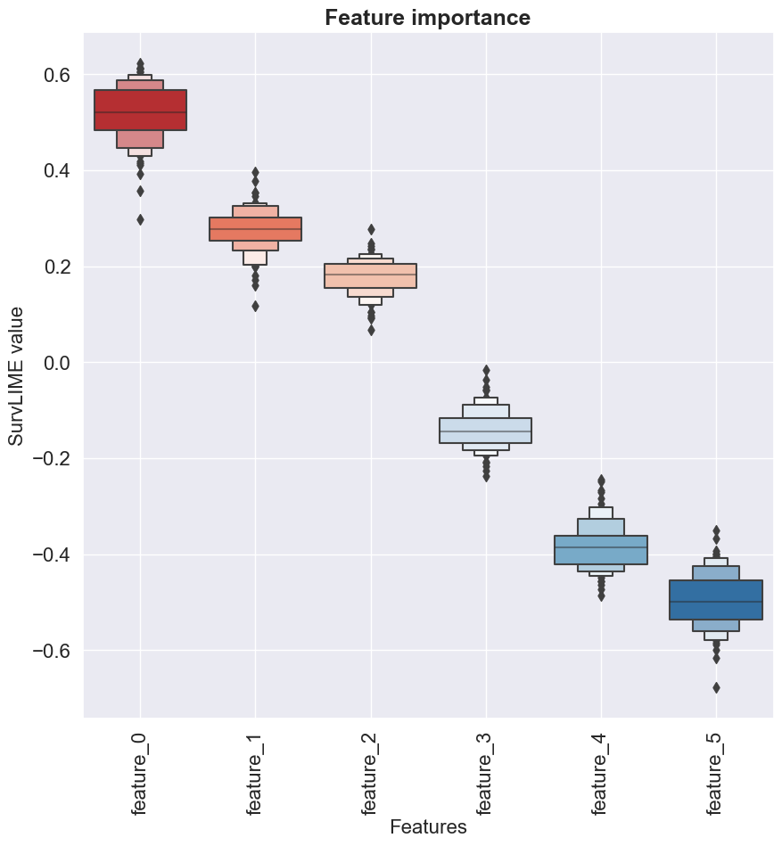
Finally, plot_montecarlo_weights() is the last functionality we have developed and it allows to create a boxen plot from the values obtained by montecarlo_explanation() method. plot_montecarlo_weights() has two optional input parameters: with_colour and figure_path. These parameters behave in the same way as the input parameters of the function plot_weights().

The following code fragment shows how to use the package to compute the importance vector for the features for a single individual. In order to run it, let us suppose we have a machine learning model already trained, denoted by model, which has a method that obtains a prediction for the Cumulative Hazard Function, model.predict_cumulative_hazard_function and it has an attribute containing the times for which the previous method provides a prediction, model.event_times_ (we are adopting the notation of sksurv package).

The individual to be explained is denoted by individual, the dataset containing the features is denoted by features, the vector containing the event indicators is denoted by events and the vector containing the times is denoted by times.

from survlimepy import SurvLimeExplainer explainer = SurvLimeExplainer( training_features=features, training_events=events, training_times=times, model_output_times=model.event_times_ )

explanation = explainer.explain_instance( data_row=individual, predict_fn=model.predict_cumulative_hazard_function, num_samples=1000 ) explainer.plot_weights()

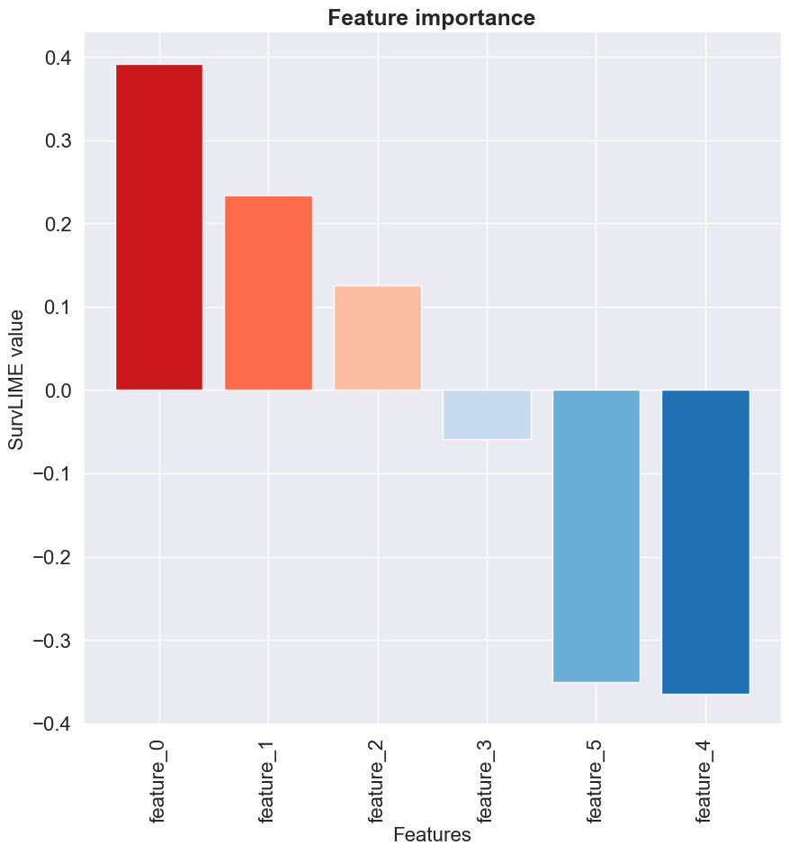
The last line displays the importance of each feature. The result is shown in Figure 1. The computed coefficients are displayed in descending order, with a red colour palette for the features that increase the Cumulative Hazard Function and a blue palette for those that decrease it. The remaining input parameters in ‘SurvLimeExplainer’ as well as in function explain_instance() use their corresponding default values.

The next code block exemplifies how to use montecarlo_explanation() to obtain a set of SurvLIME values as well as the plot_montecarlo_weights() method to display them. We make use of the same notation as before, i.e., model.predict_cumulative_hazard_function, model.event_times_, features, events and times.

Instead of explaining a single individual, we explain a set of $h$ individuals. Let, X_ind be a numpy array of size $h\times p$. For each individual, we perform 100 repetitions and, for each repetition, 1000 neighbours are generated. The code needed to obtain the results is very similar to the previous one. The last line of the code example is responsible for displaying Figure 2. Note that the variable mc_explanation is a numpy array of size $h\times p$, where the row $i$ contains the feature importance for individual $i$ in X_ind.

from survlimepy import SurvLimeExplainer explainer = SurvLimeExplainer( training_features=features, training_events=events, training_times=times, model_output_times=model.event_times_ ) mc_explanation = explainer.montecarlo_explanation( data=X_ind, predict_fn=model.predict_cumulative_hazard_function, num_repetitions=100, num_samples=1000 ) explainer.plot_montecarlo_weights()

First, two sets of data are generated randomly and uniformly in the $p$-dimensional sphere, where $p=5$. Each set is configured as follows:

• •

  Set 1: Center, $c_{1}=(0,0,0,0,0)$, radius, $r_{1}=8$, number of individuals, $n_{1}=1000$.

• •

  Set 2: Center, $c_{2}=(4,-8,2,4,2)$, radius, $r_{2}=8$, number of individuals, $n_{2}=1000$.

Using these parameters, two datasets represented by the matrices $\mathbf{X}_{r}$ of size $n_{r}\times p$ are generated ($r\in\{1,2\}$). A row from these datasets represents an individual and a column represents a feature. Therefore, $x_{ij}$ represents the value of feature $j$ for the individual $i$.

The Weibull distribution is used to generate time data (Bender et al. 2005). This distribution respects the assumption of proportional hazards, the same as the Cox Proportional Hazards Model does. The Weibull distribution is determined by two parameters: the scale, $\lambda$, and the shape, $\nu$. Given the set of data $r$, a vector of time to events (of size $n_{r}$) is generated as

where $\mathbf{u}_{r}$ is a vector of $n_{r}$ independent and identically uniform distributions in the interval $(0,1)$. Both functions, the logarithm and the exponential, are applied component-wise. As done in Kovalev et al. 2020, all times greater than 2000 are constrained to 2000. Each set $r$ has the following set of parameters:

• •

  Set 1: $\lambda_{1}=10^{-5}$, $\nu_{1}=2$, $\boldsymbol{\beta}_{1}^{\text{\tiny T}}=(10^{-6},0.1,-0.15,10^{-6},10^{-6})$.

• •

  Set 2: $\lambda_{2}=10^{-5}$, $\nu_{2}=2$, $\boldsymbol{\beta}_{2}^{\text{\tiny T}}=(10^{-6},-0.15,10^{-6},10^{-6},-0.1)$.

Note that for the first set, the second and the third features are the most important ones. On the other hand, for the second set, the second and the fifth features are the most relevant.

In order to generate the event indicator, a Bernoulli distribution, with a probability of success equal to 0.9, is used. For each set a vector (of size $n_{r}$) of independent and identically distributed random variables is obtained. Let $\boldsymbol{\delta}_{r}$ be the vector of such realisations. The random survival data of each set $r$ is represented by a triplet $\mathbf{D}_{r}=(\mathbf{X}_{r},\boldsymbol{\tau}_{r},\boldsymbol{\delta}_{r})$.

Even though the authors of the original SurvLIME paper simulated data this way, it is worth mentioning that this is not the standard procedure in Survival Analysis. The usual way to generate data consists of using two different distributions of times, $\boldsymbol{\tau}_{0}$ and $\boldsymbol{\tau}_{1}$: $\boldsymbol{\tau}_{0}$ is the censoring time and $\boldsymbol{\tau}_{1}$ is the time-to-event. Then, the vector of observed times $\boldsymbol{\tau}=(\tau_{i})$ is obtained as $\tau_{i}=\min(\tau_{0i},\tau_{1i})$. In order to generate the event indicator vector $\boldsymbol{\delta}=(\delta_{i})$, it is taken into account both vectors $\boldsymbol{\tau}_{0}$ and $\boldsymbol{\tau}_{1}$: $\delta_{i}=\mathds{1}_{\{\tau_{1i}\leq\tau_{0i}\}}$. In this way, it is obtained that $\mathsf{P}(\delta_{i}=1)=\mathsf{P}(\tau_{1i}\leq\tau_{0i})$. Nonetheless, we proceed in the same way as in the original paper so that the results can be compared.

SurvLIMEpy allows to create a random survival dataset according to the criteria described previously. The class ‘RandomSurvivalData’ manages this part.

RandomSurvivalData( center, radius, coefficients, prob_event, lambda_weibull, v_weibull, time_cap, random_seed )

• •

  center: The center of the set. It must be a Python list of length $p$.

• •

  radius: The radius of the set. It must be a float.

• •

  coefficients: The $\boldsymbol{\beta}_{r}$ vector that is involved in Expression (11). It must be a Python list of length $p$.

• •

  prob_event: The probability for the Bernoulli distribution. It must be a float in $(0,1)$.

• •

  lambda_weibull: The $\lambda_{r}$ parameter that is involved in Expression (11). It must be a float positive number.

• •

  v_weibull: The $\nu_{r}$ parameter that is involved in Expression (11). It must be a float positive number.

• •

  time_cap (optional): If the time obtained is greater than time_cap, then time_cap is used. It must be a float positive number.

• •

  random_seed (optional): Number to be used for the random seed. The user must provide a value if the results obtained must be reproducible every time the code is executed. The default is set to empty (no reproducibility needed).

This class contains the method random_survival_data(num_points) that returns the dataset. The input parameter, num_points, is an integer indicating the number of individuals, $n_{r}$, to generate. The output of this function is a tuple of three objects: (1) $\mathbf{X}_{r}$ the matrix containing the features (of size $n_{r}\times p$); (2) $\boldsymbol{\tau}_{r}$ the vector of times to event (of size $n_{r}$); (3) $\boldsymbol{\delta}_{r}$ the vector of event indicators (of size $n_{r}$).

After obtaining both datasets, they are split randomly into two parts, a training dataset, $\mathbf{D}_{r}^{train}$ and a test dataset, $\mathbf{D}_{r}^{test}$. The training dataset consists of 900 individuals, whereas the test dataset consists of 100 individuals.

For each training dataset, a Cox Proportional Hazards Model is fitted. Let $\hat{H}_{r}(\mathbf{x},t)$, $r\in\{1,2\}$, be the resulting models. The next step is to use SurvLIMEpy to obtain the importance of each feature. The test datasets, still unexploited, are used to rank the relevance of each feature. For a given test individual from set $r$, the set up for SurvLIMEpy is:

• •

  Training dataset, $\mathbf{D}=\mathbf{D}_{r}^{train}$.

• •

  Number of neighbours, $N_{r}=1000$.

• •

  Black-box model for the Cumulative Hazard Function: $\hat{H}_{r}(\mathbf{x},t)$.

• •

  Kernel function, $K(\cdot,\cdot)=$ Gaussian Radial Basis function.

Figure 3 shows the results obtained using SurvLIMEpy package to compute the coefficients. In green, the vector of real coefficients, $\boldsymbol{\beta}_{r}$, is depicted. In blue, the estimated parameters according to Cox Proportional Hazards Model, $\hat{\boldsymbol{\beta}}_{r}^{c}$. In orange, the coefficients obtained by SurvLIMEpy, $\hat{\boldsymbol{\beta}}_{r}^{s}$, $r\in\{1,2\}$. The individual to be explained is the center of the set. Note that the results we have obtained are similar to the ones obtained in the original paper of SurvLIME.

Given that the real coefficients, $\boldsymbol{\beta}_{r}$, are known, the $\ell^{2}$ distance between $\boldsymbol{\beta}_{r}$ and $\hat{\boldsymbol{\beta}}_{r}^{s}$ can be computed. In order to study the variance of SurvLIME algorithm, the previous experiment is repeated 100 times, i.e, a Monte-Carlo simulation is performed. Throughout all the simulations, the individual to be explained is the same, the center of the set.

Thus, a set of 100 distances are obtained, $\{d_{1},\dots,d_{100}\}$. From this set, the mean, the minimum and the maximum distance can be calculated. Let $\hat{\boldsymbol{\beta}}_{mean}^{s}$, $\hat{\boldsymbol{\beta}}_{min}^{s}$ and $\hat{\boldsymbol{\beta}}_{max}^{s}$ be the SurvLIME coefficients related to those distances. Doing such a Monte-Carlo simulation for all the individuals in the test datasets, $\mathbf{D}_{1}^{test}$ and $\mathbf{D}_{2}^{test}$, leads to obtain 3 different samples of SurvLIME coefficients: $\{\hat{\boldsymbol{\beta}}_{mean,1}^{s},\dots,\hat{\boldsymbol{\beta}}_{mean,100}^{s}\}$, $\{\hat{\boldsymbol{\beta}}_{min,1}^{s},\dots,\hat{\boldsymbol{\beta}}_{min,100}^{s}\}$ and $\{\hat{\boldsymbol{\beta}}_{max,1}^{s},\dots,\hat{\boldsymbol{\beta}}_{\max,100}^{s}\}$.

Figure 4 shows the boxen plots for the three previous sets of coefficients. The left plots depict the boxen plot for the mean coefficient; the middle plots are for the minimum coefficient; the right ones correspond to the maximum coefficient. The results show that the coefficients of SurvLIME were close to the real coefficients for both sets of data. Furthermore, the mean values of the computed coefficients behave similarly to the best approximations and they show a low variance.

In the worst case scenario, SurvLIME does not behave as well as in the other two scenarios. The variance of the SurvLIME coefficients is much higher, especially for the second set of data. However, the bias is as good as the bias of the other two scenarios.

Now, we test our implementation on three open-access datasets. Each dataset is presented together with a bivariate analysis. For categorical features, the percentage of individuals that experienced the event is computed for each category. Continuous features are categorised according to their quartiles, and the resulting categorical features are described as before.

The first dataset is the UDCA dataset (Lindor et al. 1994). It contains individuals with primary biliary cirrhosis (PBC) that were randomised for treatment with ursodeoxycholic acid (UDCA). A total of $9.46\%$ of the individuals experienced the event. The features of this dataset are:

• •

  trt (categorical): Treatment received. 0 is for placebo and 1 is for UDCA.

• •

  stage (categorical): Stage of disease. 0 is for better and 1 is for worse.

• •

  bili (continuous): Bilirubin value at entry.

• •

  riskscore (continuous): The Mayo PBC risk score at entry.

Note that the UDCA dataset contains an individual whose riskscore is missing. We drop this individual from the dataset. The bivariate descriptive analysis is displayed in Table 1.

The second dataset is the LUNG dataset (Loprinzi et al. 1994). It contains individuals with advanced lung cancer from the North Central Cancer Treatment Group. A total of $70.33\%$ of the individuals experienced the event. The features of this dataset are:

• •

  inst (categorical): Institution code. The institutions are coded with numbers between 1 and 33.

• •

  sex (categorical): Gender. 1 is for male and 2 is for female.

• •

  ph.ecog (categorical): ECOG performance score as rated by the physician. The categories are:

  • –

    0: Asymptomatic.

  • –

    1: Symptomatic but completely ambulatory.

  • –

    2: In bed <50% of the day.

  • –

    3: In bed > 50% of the day but not bedbound.

• •

  age (continuous): Age of the individual.

• •

  ph.karno (continuous): Karnofsky performance score rated by physician.

• •

  pat.karno (continuous): Karnofsky performance score as rated by the individual.

• •

  meal.cal (continuous): Calories consumed at meals.

• •

  wt.loss (continuous): Weight loss in last six months.

We drop some information regarding LUNG dataset. First, we do not use the feature inst because it does not provide any further information allowing institutions identification. Second, we remove the meal.cal feature, since it contains a total of 20.6% of missing values. Third, 18 individuals have at least one feature with missing information. We drop those individuals from the dataset. Finally, with regards the feature ph.ecog, just a single individual is in the category 3. We do not consider this individual, therefore we drop it. After this preprocessing, we are left with 209 individuals.

As for the UDCA dataset, a bivariate descriptive analysis is performed in LUNG dataset. Table 2 contains the results. Those features dropped from the dataset are not included in that table.

The last dataset is the Veteran dataset (Kalbfleisch and Prentice 2002) which consists of individuals with advanced inoperable Lung cancer. The individuals were part of a randomised trial of two treatment regimens. The event of interest for the three datasets is the individual’s death. A total of $93.43\%$ of the individuals experienced the event. The features of this dataset are:

• •

  trt (categorical): Treatment received. 1 is for standard and 2 is for test.

• •

  prior (categorical): It indicates if the patient has received another therapy before the current one. 0 means no and 10 means yes.

• •

  celltype(categorical): Histological type of the tumor. The categories are: squamous, smallcell, adeno and large.

• •

  karno (continuous): Karnofsky performance score.

• •

  age (continuous): Age of the individual.

• •

  diagtime (continuous): Months from diagnosis to randomisation.

Note that the Veteran dataset does not contain any missing value. The results of the bivariate descriptive analysis for the Veteran dataset are displayed in Table 3.

Table 4 shows a brief summary of each dataset: $p$ corresponds to the number of features, while $p^{*}$ is the number of features after pre-processing (dropping and doing one-hot-encoding), $n$ denotes the number of individuals of the dataset, and $n_{full}$ is the number of individuals once the missing values are dropped.

We model the event of interest by means of machine learning algorithms. Given a dataset $\mathbf{D}$, it is divided randomly into two sets: a training dataset, $\mathbf{D}^{train}$, and a test dataset, $\mathbf{D}^{test}$, using $90\%$ of individuals for training and $10\%$ for testing.

Once the data is split, we preprocess $\mathbf{D}^{train}$. We apply one-hot-encoding to categorical features. If a categorical feature has $k$ categories, then we create $k-1$ binary features. The category without a binary feature is the reference category. After that, the original feature is deleted from the dataset since we use the $k-1$ new features treated as continuous ones. Continuous features are also preprocessed. Given $\mathbf{\tilde{x}}_{j}$, we first estimate the mean, $\hat{\mu}^{j}_{train}$, and the standard deviation, $\hat{\sigma}^{j}_{train}$. Then, the standarisation performed is $(\mathbf{\tilde{x}}_{j}-\hat{\mu}^{j}_{train})/\hat{\sigma}^{j}_{train}$. This new feature is used instead of $\mathbf{\tilde{x}}_{j}$.

The same preprocess is applied on $\mathbf{D}^{test}$. Note that the parameters that involve the preprocess (for both, categorical and continuous features) are taken from the preprocess performed on $\mathbf{D}^{train}$, i.e., nothing is estimated in the test set. Let $\mathbf{\tilde{D}}^{train}$ and $\mathbf{\tilde{D}}^{test}$ be the datasets obtained after preprocessing them.

Afterwards, a model is trained in $\mathbf{\tilde{D}}^{train}$ and $\mathbf{\tilde{D}}^{test}$ is used to obtain the c-index value, a goodness-of-fit measure for survival models (see Appendix A for more details about c-index and Survival Analysis).

In this section, we use five distinct machine learning algorithms: the Cox Proportional Hazards Model (CoxPH), Random Survival Forest (RSF) (both from sksurv package), eXtreme Gradient Boosted Survival Trees (XGB) (from xgbse package) as well as continuous and time-discrete deep learning models, DeepSurv and DeepHit (both from pycox package). We have performed an hyperparameter tuning strategy for each model and dataset.

Having trained a model, SurvLIMEpy is applied to obtain feature importance. For a given individual $i$ of $\mathbf{\tilde{D}}^{test}$, SurvLIME algorithm is used 100 times, which produces a set of 100 coefficients: $\{\hat{\boldsymbol{\beta}}_{i,1}^{s},\dots,\hat{\boldsymbol{\beta}}_{i,100}^{s}\}$. Then, the mean value across all the simulation is calculated, $\bar{\boldsymbol{\beta}}_{i}^{s}=(1/100)\sum_{j=1}^{100}\hat{\boldsymbol{\beta}}_{i,j}^{s}$. That vector, $\bar{\boldsymbol{\beta}}_{i}^{s}$, is used as the feature importance for the individual $i$. This process is applied to all the individuals in the test dataset. Therefore, a set of coefficients $\{\bar{\boldsymbol{\beta}}_{1}^{s},\dots,\bar{\boldsymbol{\beta}}_{n_{t}}^{s}\}$ is obtained, where $n_{t}$ is the total number of individuals in the test dataset. This set of coefficients is used in this study. Note that for UDCA $n_{t}$ is equal to 17, for LUNG it is equal to 21, and for Veteran it is equal to 14.

References

- Cox [1972] David R Cox. Regression models and life-tables. Journal of the Royal Statistical Society: Series B (Methodological), 34(2):187–202, 1972.
- Ishwaran et al. [2008] Hemant Ishwaran, Udaya B. Kogalur, Eugene H. Blackstone, and Michael S. Lauer. Random survival forests. The Annals of Applied Statistics, 2(3):841 – 860, 2008. doi: 10.1214/08-AOAS169. URL https://doi.org/10.1214/08-AOAS169.
- Barnwal et al. [2022] Avinash Barnwal, Hyunsu Cho, and Toby Hocking. Survival regression with accelerated failure time model in xgboost. Journal of Computational and Graphical Statistics, 0(0):1–11, 2022. doi: 10.1080/10618600.2022.2067548. URL https://doi.org/10.1080/10618600.2022.2067548.
- Lee et al. [2018] Changhee Lee, William Zame, Jinsung Yoon, and Mihaela van der Schaar. Deephit: A deep learning approach to survival analysis with competing risks. Proceedings of the AAAI Conference on Artificial Intelligence, 32(1):–, Apr. 2018. doi: 10.1609/aaai.v32i1.11842. URL https://ojs.aaai.org/index.php/AAAI/article/view/11842.
- Katzman et al. [2018] Jared Katzman, Uri Shaham, Alexander Cloninger, Jonathan Bates, Tingting Jiang, and Yuval Kluger. Deepsurv: Personalized treatment recommender system using a cox proportional hazards deep neural network. BMC Medical Research Methodology, 18:–, 02 2018. doi: 10.1186/s12874-018-0482-1.
- Wang et al. [2019] Ping Wang, Yan Li, and Chandan K Reddy. Machine learning for survival analysis: A survey. ACM Computing Surveys (CSUR), 51(6):1–36, 2019.
- Spooner et al. [2020] Annette Spooner, Emily Chen, Arcot Sowmya, Perminder Sachdev, Nicole A Kochan, Julian Trollor, and Henry Brodaty. A comparison of machine learning methods for survival analysis of high-dimensional clinical data for dementia prediction. Scientific reports, 10(1):1–10, 2020.
- Hao et al. [2021] Lin Hao, Juncheol Kim, Sookhee Kwon, and Il Do Ha. Deep learning-based survival analysis for high-dimensional survival data. Mathematics, 9(11):1244, 2021.
- Barredo Arrieta et al. [2020] Alejandro Barredo Arrieta, Natalia Díaz-Rodríguez, Javier Del Ser, Adrien Bennetot, Siham Tabik, Alberto Barbado, Salvador Garcia, Sergio Gil-Lopez, Daniel Molina, Richard Benjamins, Raja Chatila, and Francisco Herrera. Explainable artificial intelligence (xai): Concepts, taxonomies, opportunities and challenges toward responsible ai. Information Fusion, 58:82–115, 2020. ISSN 1566-2535. doi: https://doi.org/10.1016/j.inffus.2019.12.012. URL https://www.sciencedirect.com/science/article/pii/S1566253519308103.
- Ribeiro et al. [2016] Marco Tulio Ribeiro, Sameer Singh, and Carlos Guestrin. Why should i trust you? explaining the predictions of any classifier. In Proceedings of the 22nd ACM SIGKDD international conference on knowledge discovery and data mining, pages 1135–1144. ACM, 2016.
- Lundberg and Lee [2017] Scott M Lundberg and Su-In Lee. A unified approach to interpreting model predictions. Advances in neural information processing systems, 30, 2017.
- Barr Kumarakulasinghe et al. [2020] Nesaretnam Barr Kumarakulasinghe, Tobias Blomberg, Jintai Liu, Alexandra Saraiva Leao, and Panagiotis Papapetrou. Evaluating local interpretable model-agnostic explanations on clinical machine learning classification models. In 2020 IEEE 33rd International Symposium on Computer-Based Medical Systems (CBMS), pages 7–12, 2020. doi: 10.1109/CBMS49503.2020.00009.
- Kovalev et al. [2020] Maxim S. Kovalev, Lev V. Utkin, and Ernest M. Kasimov. Survlime: A method for explaining machine learning survival models. Knowledge-Based Systems, 203:106164, 2020. ISSN 0950-7051. doi: https://doi.org/10.1016/j.knosys.2020.106164. URL https://www.sciencedirect.com/science/article/pii/S0950705120304044.
- Krzyziński et al. [2023] Mateusz Krzyziński, Mikołaj Spytek, Hubert Baniecki, and Przemysław Biecek. Survshap(t): Time-dependent explanations of machine learning survival models. Knowledge-Based Systems, 262:110234, 2023. ISSN 0950-7051. doi: https://doi.org/10.1016/j.knosys.2022.110234. URL https://www.sciencedirect.com/science/article/pii/S0950705122013302.
- Spytek et al. [2022] Mikołaj Spytek, Mateusz Krzyziński, Hubert Baniecki, and Przemysław Biecek. survex: Explainable Machine Learning in Survival Analysis. R package version 0.2.2, 2022. URL https://github.com/ModelOriented/survex.
- Diamond and Boyd [2016] Steven Diamond and Stephen Boyd. CVXPY: A Python-embedded modeling language for convex optimization. Journal of Machine Learning Research, 17(83):1–5, 2016.
- Stellato et al. [2020] B. Stellato, G. Banjac, P. Goulart, A. Bemporad, and S. Boyd. OSQP: an operator splitting solver for quadratic programs. Mathematical Programming Computation, 12(4):637–672, 2020. doi: 10.1007/s12532-020-00179-2. URL https://doi.org/10.1007/s12532-020-00179-2.
- Molnar [2022] Christoph Molnar. Interpretable Machine Learning. https://christophm.github.io/interpretable-ml-book/, 2 edition, 2022. URL https://christophm.github.io/interpretable-ml-book.
- Silverman [1986] B. W. Silverman. Density estimation for statistics and data analysis. Chapman and Hall London ; New York, 1986. ISBN 0412246201.
- Utkin et al. [2020] Lev V Utkin, Maxim S Kovalev, and Ernest M Kasimov. Survlime-inf: A simplified modification of survlime for explanation of machine learning survival models. arXiv preprint arXiv:2005.02387, 2020.
- Pölsterl [2020] Sebastian Pölsterl. scikit-survival: A library for time-to-event analysis built on top of scikit-learn. Journal of Machine Learning Research, 21(212):1–6, 2020. URL http://jmlr.org/papers/v21/20-729.html.
- Vieira et al. [2020] Davi Vieira, Gabriel Gimenez, Guilherme Marmerola, and Vitor Estima. Xgboost survival embeddings: improving statistical properties of xgboost survival analysis implementation, 2020. URL http://github.com/loft-br/xgboost-survival-embeddings.
- Kvamme et al. [2019] Håvard Kvamme, Ørnulf Borgan, and Ida Scheel. Time-to-event prediction with neural networks and cox regression. arXiv preprint arXiv:1907.00825, 2019.
- Aalen [1978] Odd Aalen. Nonparametric inference for a family of counting processes. The Annals of Statistics, pages 701–726, 1978.
- Bender et al. [2005] Ralf Bender, Thomas Augustin, and Maria Blettner. Generating survival times to simulate cox proportional hazards models. Statistics in medicine, 24(11):1713–1723, 2005.
- Lindor et al. [1994] K D Lindor, E R Dickson, W P Baldus, R A Jorgensen, J Ludwig, P A Murtaugh, J M Harrison, R H Wiesner, M L Anderson, and S M Lange. Ursodeoxycholic acid in the treatment of primary biliary cirrhosis. Gastroenterology, 106(5):1284–1290, May 1994.
- Loprinzi et al. [1994] Charles Lawrence Loprinzi, John A Laurie, H Sam Wieand, James E Krook, Paul J Novotny, John W Kugler, Joan Bartel, Marlys Law, Marilyn Bateman, and Nancy E Klatt. Prospective evaluation of prognostic variables from patient-completed questionnaires. north central cancer treatment group. Journal of Clinical Oncology, 12(3):601–607, 1994.
- Kalbfleisch and Prentice [2002] J. D. Kalbfleisch and Ross L. Prentice. The statistical analysis of failure time data. Wiley series in probability and statistics. J. Wiley, Hoboken, N.J, 2nd ed edition, 2002. ISBN 978-0-471-36357-6.
- Hosmer and Lemeshow [1999] David W Hosmer and Stanley Lemeshow. Applied survival analysis: time-to-event, volume 317. Wiley-Interscience, 1999.
- Prinja et al. [2010] Shankar Prinja, Nidhi Gupta, and Ramesh Verma. Censoring in clinical trials: review of survival analysis techniques. Indian journal of community medicine: official publication of Indian Association of Preventive & Social Medicine, 35(2):217, 2010.
- Harrell [2006] Frank E. Harrell. Regression Modeling Strategies. Springer-Verlag, Berlin, Heidelberg, 2006. ISBN 0387952322.
- Harrell et al. [1982] Frank E. Harrell, Robert M. Califf, David B. Pryor, Kerry L. Lee, and Robert A. Rosati. Evaluating the Yield of Medical Tests. JAMA, 247(18):2543–2546, 05 1982. ISSN 0098-7484. doi: 10.1001/jama.1982.03320430047030. URL https://doi.org/10.1001/jama.1982.03320430047030.
- Harrell et al. [1996] Frank E. Harrell, Kerry L Lee, and Daniel B Mark. Multivariable prognostic models: issues in developing models, evaluating assumptions and adequacy, and measuring and reducing errors. Statistics in medicine, 15(4):361–387, 1996.
Appendix A Survival Analysis
Survival Analysis, also known as time-to-event analysis, is a branch of Statistics that studies the time until a particular event of interest occurs [Hosmer and Lemeshow 1999, Kalbfleisch and Prentice 2002]. It was initially developed in biomedical sciences and reliability engineering but, nowadays, it is used in a plethora of fields. A key point of a Survival Analysis approach is that each individual is represented by a triplet , where is the vector of features, indicates time to event or lost to follow-up time of the individual (it is assumed to be non-negative and continuous) and is the event indicator denoting whether the event of interest has been observed or not.
Given a dataset consisting of triplets , , where is the number of individuals, Survival Analysis aims to build a model , that allows to estimate the risk a certain individual experiences the event at a certain time . This risk estimator is given by .
A.1 Censoring
Censoring is a crucial phenomenon of Survival Analysis. It occurs when some information about individual survival time is available, but we do not know the exact survival time. It results in the event of interest not being observed for some individuals. This might happen when the event is not observed during the time window of the study, or the individual dropped out of the study by other uninterested causes. If this takes place, the individual is considered censored and . The three main types of censorship are:
- •
Right-censoring is said to occur when, despite continuous monitoring of the outcome event, the individual is lost to follow-up, or the event does not occur within the study duration [Prinja et al. 2010].
Left-censoring happens if an individual had been on risk for the event of interest for a period before entering the study.
Interval-censoring applies to individuals when the time until the event of interest is not known precisely (and instead, only is known to fall into a particular interval).
From the three of them, right-censoring, followed by interval-censoring, are the two most common types of censoring. Left-censoring is sometimes ignored since the starting point is defined by an event such as the entry of a individual into the study.
If the event of interest is observed for individual , and correspond to the time from the beginning of the study to the event’s occurrence respectively. This is also called an uncensored observation.
On the other hand, if the instance event is not observed or its time to event is greater than the observation window, corresponds to the time between the beginning of the study and the end of observation. In this case, the event indicator is , and the individual is considered to be censored.
A.2 Survival Function
The Survival Function is one of the main concepts in Survival Analysis, it represents the probability that the time to event is not earlier than time which is the same as the probability that a individual survives past time without the event happening. It is expressed as: