Quantifying the Energy Relaxation Rate of Quantum States Using D-Wave Device and the Discovery of Long-Lived Multiqubit States Preprint: APS/123-QED

Takashi Imoto Email: takashi.imoto@aist.go.jp Affiliation: Research Center for Emerging Computing Technologies, National Institute of Advanced Industrial Science and Technology (AIST), 1-1-1 Umezono, Tsukuba, Ibaraki 305-8568, Japan. Yuki Susa Email: y-susa@nec.com Affiliation: Secure System Platform Research Laboratories, NEC Corporation, Kawasaki, Kanagawa 211-8666, Japan Affiliation: NEC-AIST Quantum Technology Cooperative Research Laboratory, National Institute of Advanced Industrial Science and Technology (AIST), Tsukuba, Ibaraki 305-8568, Japan Ryoji Miyazaki Email: miyazaki-aj@nec.com Affiliation: Secure System Platform Research Laboratories, NEC Corporation, Kawasaki, Kanagawa 211-8666, Japan Affiliation: NEC-AIST Quantum Technology Cooperative Research Laboratory, National Institute of Advanced Industrial Science and Technology (AIST), Tsukuba, Ibaraki 305-8568, Japan Yuichiro Matsuzaki Email: ymatsuzaki872@g.chuo-u.ac.jp Affiliation: Department of Electrical, Electronic, and Communication Engineering, Faculty of Science and Engineering, Chuo University

August 11, 2026

Abstract

Quantum annealing has been demonstrated with superconducting qubits. Such a quantum annealer has been used to solve combinatorial optimization problems. Moreover, it serves as a quantum simulator for investigating the properties of quantum many-body systems. However, the coherence properties of multi-qubit states provided by D-Wave Quantum Inc. have not been explored sufficiently. Here, using the D-Wave device, we measure the energy relaxation rate of superconducting qubits and find long-lived multi-qubit states. Specifically, we investigate the energy relaxation rate of the first excited states of a fully connected Ising model with a transverse field. We find that the decay rate of the excited states of such a system with four qubits is orders of magnitude smaller than that of the excited state of a single qubit, which demonstrates the existence of long-lived multi-qubit states. We elucidate the mechanism using an independent decoherence model that qualitatively describes the phenomenon. In addition, by using such a mechanism, we theoretically predict a long-lived entangled state whose energy relaxation rate is smaller than that of the separable states.

I Introduction

Quantum annealing(QA), which has witnessed significant developments, is useful for solving combinatorial optimization problems Kadowaki and Nishimori 1998; Farhi et al. 2000; Farhi et al. 2001. D-Wave Quantum Inc. has developed a quantum annealing machine that consists of thousands of qubits Johnson et al. 2011. The combinatorial optimization problem can be mapped into a search for the ground state of the Ising Hamiltonian Lucas 2014; Lechner et al. 2015. Efficient clustering and machine learning using QA have been reported in the literatureKurihara et al. 2014; Kumar et al. 2018; Amin 2015; Neven et al. 2008; Korenkevych et al. 2016; Benedetti et al. 2017; Willsch et al. 2020; Wilson et al. 2021. Moreover, QA is useful for topological data analysis (TDA)Berwald et al. 2018.

Furthermore, a quantum annealing machine can be used not only for solving problems but also as a quantum simulator for quantum many-body systems in and out of equilibrium King et al. 2018; Kairys et al. 2020; Harris et al. 2018; Zhou et al. 2021. There is considerable interest in the potential of D-Wave machines to exploit quantum properties, and recent experiments with a D-Wave machine have shown good agreement with theoretical predictions based on the Schrödinger dynamics King et al. 2022a; King et al. 2022b. To this end, a study has attempted to use longitudinal magnetic fields to probe the dynamics of a qubit and distinguish the effects of noise in the D-Wave machineMorrell et al. 2022. Tunneling spectroscopy Berkley et al. 2013 is a way to estimate the energy gap of the transverse-field Ising Hamiltonian, and numerical simulations of open quantum systems have been performed to reproduce the results of the tunneling spectroscopy by using the D-Wave machine Chen and Lidar 2020. When reverse quantum annealing was performed to search doubly degenerate ground states, the probability of finding one of the ground states was much larger than that of the other state, and this behavior was qualitatively reproduced by a theoretical model of decoherence Bando et al. 2022.

Quantum correlation plays an important role in a quantum simulator. Experimental and theoretical results indicate that correlation among qubits lessens the impact of noise during QA Weinberg et al. 2020. Especially since an eigenstate of the Hamiltonian provided by the D-Wave machine can be entangled, it is important to study the coherence properties of entangled states. The properties of the entanglement of the ground state during QA were experimentally and theoretically investigated Lanting et al. 2014; Albash et al. 2015. However, the coherence properties of multi-qubit states generated by D-Wave have not been sufficiently explored.

In this paper, we measure the energy relaxation rate of the excited states during QA by using the D-Wave machine. We employ a fully connected Ising model of four qubits for the problem Hamiltonian of QA. Further, we show that the energy relaxation rate of the first excited states of such a four-qubit system is much smaller than that of a single-qubit system. We elucidate the mechanism of this phenomenon by using an independent decoherence model. Moreover, by adopting such a mechanism, we theoretically predict the existence of long-lived entanglement whose energy relaxation rate is smaller than that of the separable states under the effect of independent decoherence.

II Experimental Results using D-Wave machine

II.1 $T_{1}$ Measurement Setup

First, we explain the method for measuring the energy relaxation rate of the excited states during QA by using a D-Wave machine. Our method is similar to that used in Ref. Harris et al. 2008 where an energy relaxation rate of a single rf SQUID is measured. On the other hand, our method allows us to measure the energy relaxation rate of the interacting qubits. We perform the reverse quantum annealing (RQA) with a hot start where the initial state is the first excited state of the problem Hamiltonian, and we investigate the energy relaxation rate of the state during RQA. We remark that we use the D-Wave Advantage system 6.4 for our demonstration throughout this paper. Although embedding techniques have been developed for a large number of qubits Yang and Dinneen 2016; Okada et al. 2019; Boothby et al. 2020; Cai et al. 2014; Klymko et al. 2014; Boothby et al. 2016; Zaribafiyan et al. 2017, we employ a fully connected Ising model with four qubits, which is the maximum system size without embedding. Moreover, we use several varieties of qubits in the D-Wave machine.

Figure 1: Scheduling functions

A(s)

and

B(s)

for the D-Wave device. This plot illustrates the amplitude of the scheduling functions

A(s)

and

B(s)

against the dimensionless parameter

s

, which ranges from

0

1

. A(s) represents the amplitude of the transverse magnetic field, whereas

B(s)

corresponds to the combined amplitude of the longitudinal magnetic field and Ising Hamiltonian.

Refer to caption — Figure 2: Schduling function of the reverse quantum annealing (RQA) against time $t$ to investigate energy relaxation rate in D-Wave Systems. The scheduling is divided into three distinct phases: $t_{1}$ , $t_{2}$ , and $t_{3}$ . During $0<t<t_{1}$ , $s$ linearly decreased from 1 to $h_{d}$ . In $t_{1}<t<t_{2}$ , $s$ is constant against time $t$ . During $t_{2}<t<t_{3}$ , $s$ linearly increases back to $1$ , facilitating the measurement of the energy relaxation rate of the excited state. If we assume that non-adiabatic transitions during $0<t<t_{1}$ and $t_{2}<t<t_{3}$ are negligible, the relationship between the survival probability and $t_{2}$ can be used to determine the energy relaxation rate.

The Hamiltonian is given as follows:

$\displaystyle H(s)$	$\displaystyle=\frac{A(s)}{2}H_{D}+\frac{B(s)}{2}\biggl(g(s)H_{L}+H_{P}\biggr)$	(1)
$\displaystyle H_{P}$	$\displaystyle=-J\sum_{j<k}\sigma_{j}^{(z)}\sigma_{k}^{(z)}$	(2)
$\displaystyle H_{L}$	$\displaystyle=\frac{h}{2}\sum_{j=1}^{N}\sigma_{j}^{(z)}$	(3)
$\displaystyle H_{D}$	$\displaystyle=-B\sum_{j=1}^{N}\sigma_{j}^{(x)},$	(4)

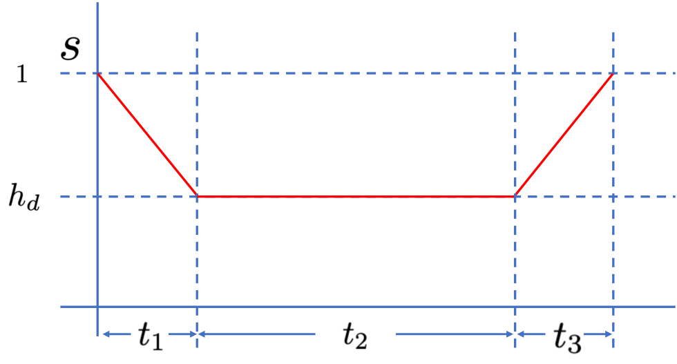
where $H_{P}$ denotes the problem Hamiltonian, $H_{D}$ denotes the drive Hamiltonian, $H_{L}$ denotes the Hamiltonian of the longitudinal magnetic field, $B$ ( $h$ ) denotes the amplitude of the transverse (horizontal) magnetic fields, $J$ denotes the coupling strength, and $s$ denotes the time-dependent parameter for controlling the QA schedule. In this paper, we set $g(s)=1$ . The scheduling functions $A(s)$ and $B(s)$ for the D-Wave Advantage system 6.4 are given as shown in Fig. 1. Throughout our paper, we set $h=1$ [GHz] and $B=1$ [GHz] unless specified otherwise. Furthermore, when we consider a fully connected Ising model, we set $J=1$ and $N=4$ . By contrast, when we consider a non-interacting model (or a single-qubit model), we set $J=0$ and $N=1$ for simplicity. We select the first excited state of the problem Hamiltonian as an initial state. For the fully connected Ising model, the all-up state $\ket{\uparrow\uparrow\uparrow\uparrow}$ is the first excited state. The schedule of the Hamiltonian is described as follows. (See Fig. 2) First, from $t=0$ to $t=t_{1}$ , we change the parameter of the Hamiltonian from $s=1$ to $s=h_{d}$ as a linear function of $t$ , where we can control the strength of the transverse magnetic fields by tuning $h_{d}$ . Second, from $t=t_{1}$ to $t=t_{1}+t_{2}$ , we let the Hamiltonian remain in the same form at $s=h_{d}$ . Third, from $t=t_{1}+t_{2}$ to $t=t_{1}+t_{2}+t_{3}$ , we gradually change the parameter of the Hamiltonian from $s=h_{d}$ to $s=1$ . Fourth, we measure the state with a computational basis. Finally, we repeat this protocol with various values of $t_{2}$ . We obtain the survival probability of the initial state after these processes. We fit the survival probability by using $ce^{-\Gamma t_{2}}$ where $c$ is a constant factor, and we estimate the energy relaxation rate $\Gamma$ . Throughout this paper, we set $t_{1}=t_{3}=1$ $\mu$ s, the annealing times $t_{1}$ and $t_{3}$ are set to be $1$ $\mu$ s, and we define an energy relaxation time as the inverse of the energy relaxation rate.

II.2 Experimental Results

Using the method described above, we measure the energy relaxation rate of the first excited state. Moreover, we compare the energy relaxation rate of the state of the transverse-field Ising model with that of the single-qubit model. Fig. 3 (a) shows the survival probability plotted against $t_{2}$ in the case of the fully connected Ising model with the transverse field. As can be seen, the survival probability decays exponentially. Furthermore, as $h_{d}$ is decreased, the energy relaxation rate becomes larger. Fig. 3 (b) shows the survival probability plotted against $t_{2}$ in the case of the single-qubit model. Similar to the case of the fully connected Ising model, the energy relaxation rate becomes larger as $h_{d}$ is decreased. Importantly, the energy relaxation rate of the state of the single-qubit model is larger than that of the fully connected Ising model with the transverse field. The details of the experimental data regarding the measured energy relaxation time are presented in Appendix A. To gain a deeper understanding of what occurs in the RQA, we perform numerical calculations in section III.2. We will discuss the origin of the long-lived multi-qubit state in section II.3. Additionally, the survival probability is plotted against $h_{d}$ in Fig. 4. Again, we confirm that the survival probability in the case of the fully connected Ising model is higher than that in the case of the non-interacting model. These experimental results demonstrate that the energy relaxation time of the multi-qubit states can be longer than that of the single-qubit state.

Here, we discuss the possible origin of the decoherence in our experiments. For a superconducting flux qubit composed of three Josephson junctions Chiorescu et al. 2003; Van Der Wal et al. 2000; Mooij et al. 1999, the main source of decoherence is the change in the magnetic flux that penetrates the superconducting loop Yoshihara et al. 2006; Kakuyanagi et al. 2007. This induces the fluctuation of the amplitude of $\hat{\sigma}_{z}$ . Moreover, low-frequency flux noise was observed for the RF-SQUID Harris et al. 2008; Lanting et al. 2009; Harris et al. 2010, and the flux fluctuations induce the change in the amplitude of $\hat{\sigma}_{z}$ . From the aforementioned observations, we infer that the qubits in the D-Wave machine are also affected by the amplitude fluctuation of $\hat{\sigma}_{z}$ . Our results show that the multi-qubit states are robust against energy relaxation induced by such fluctuations. To reveal the origin of the long-lived multi-qubit states, we consider the analysis with the Redfield master equation in the following subsection.

II.3 Perturbative analysis for the long-lived qubit

II.3.1 Analysis with the Redfield master equation

To investigate the energy relaxation rate of the first excited state, we consider the Bloch-Redfield master equation defined as

	$\displaystyle\frac{d}{dt}$	$\displaystyle\rho(t)=-i[H(s(t)),\rho(t)]+\sum_{k,l}\sum_{\omega,\omega^{\prime}}e^{i(\omega-\omega^{\prime})}\gamma_{kl}(\omega^{\prime})$
		$\displaystyle\times\biggl\{A_{l}(\omega^{\prime})\rho(t)A_{k}^{{\dagger}}(\omega)-A_{k}^{{\dagger}}(\omega)A_{l}(\omega^{\prime})\rho(t)\biggr\}+h.c$		(5)

where $\omega$ denotes the eigen energy difference of $H$ , $\hat{A}_{k}$ denotes noise operator on the $k$ -th qubit, $A_{k}(\omega)=\sum_{\epsilon^{\prime}-\epsilon=\omega}\ket{\psi_{\epsilon}}\bra{\psi_{\epsilon}}A_{k}\ket{\psi_{\epsilon'}}\bra{\psi_{\epsilon'}}$ denotes the noise operator associated with $\omega$ , $\epsilon$ denotes the eigenvalue of the Hamiltonian $H(t)$ , $\ket{\psi_{\epsilon}}$ denotes the eigenvector of the Hamiltonian $H(t)$ , and $\gamma_{kl}(\omega)$ denotes the power spectrum density. We set $\hat{\sigma}^{(z)}_{k}$ as the noise operator of $A_{k}$ . Also, we assume independent noise such as $\gamma_{kl}(\omega)\propto\delta_{k,l}$ .

In the low-temperature limit, only transitions from the first excited state to the ground state need to be considered. Consequently, noise operators can be expressed as

	$\displaystyle A_{k}(\omega)=$	$\displaystyle\ket{\phi_{gs}}\bra{\phi_{gs}}A_{k}\ket{\phi_{1st}}\bra{\phi_{1st}}$
	$\displaystyle=$	$\displaystyle(\bra{\phi_{gs}}A_{k}\ket{\phi_{1st}})\ket{\phi_{gs}}\bra{\phi_{1st}}.$		(6)

Here, $\ket{\phi_{gs}}\bra{\phi_{1st}}$ represents the transition operator from the first excited state to the ground state, while the transition matrix element $\bra{\phi_{gs}}A_{k}\ket{\phi_{1st}}$ characterized the strength of the transition. Furthermore, incorporating the effect of the power spectral density from Eq. (5), the relaxation rate can be evaluated as

\displaystyle\tilde{\Gamma}=\sum_{j=1}^{L}\sqrt{\gamma_{j}(\omega)}|\bra{\phi_{gs}}\hat{\sigma}_{j}^{(z)}\ket{\phi_{1st}}|^{2}.

(7)

We note that $\tilde{\Gamma}$ depends on the transition matrix and the energy gap between the ground state and the first excited state in the system Hamiltonian.

II.3.2 Perturbative analysis for the long-lived qubit

The decoherence rate depends on the power spectral density and the transition matrix such as $|\bra{\phi_{gs}}\hat{\sigma}_{j}^{(z)}\ket{\phi_{1st}}|$ as the previous section. This suggests that the transition matrix plays a crucial role in determining the energy relaxation rate if the energy gap is the same.

To elucidate the mechanism of the low energy relaxation rate of multi-qubit states, we employ perturbation theory and obtain the analytical form of the ground state when the transverse magnetic field is small. Accordingly, the transition matrix provides a way to quantitatively evaluate the robustness of the first excited state against decoherence Hornberger 2009a, based on the Redfield master equation.

We rewrite the total Hamiltonian (1) as follows:

\displaystyle H=H_{0}+\lambda H_{1}.

(8)

where $H_{1}$ is the perturbative Hamiltonian and $H_{0}$ is the unpertabative Hamiltonian. These Hamiltonians are defined by

	$\displaystyle H_{0}$	$\displaystyle=H_{P}+H_{L},$		(9)
	$\displaystyle H_{1}$	$\displaystyle=H_{D},$		(10)

where we set the amplitude of the transverse magnetic field $B=1$ .

Let us define $\hat{S}^{(a)}=\sum_{j=1}^{4}\hat{\sigma}_{j}^{(a)}\ (a=x,y,z)$ and $S^{(z)}$ as the eigenvalue of $\hat{S}_{z}$ . We consider the fully symmetric representation corresponding to the maximum total spin, and the subspace is spanned by the Dicke states. In this subspace, we can specify the state by $S^{(z)}$ .

Using perturbation theory, we describe the $n$ -th excited state as follows:

\displaystyle\ket{\phi_{n}}

\displaystyle=\ket{\phi_{n}^{(0)}}+\lambda\sum_{m\neq n}\frac{\bra{\phi_{m}^{(0)}}H_{D}\ket{\phi_{n}^{(0)}}}{E_{m}^{(0)}-E_{n}^{(0)}}\ket{\phi_{m}^{(0)}}+o(\lambda^{2}),

(11)

where $\ket{\phi_{m}^{(0)}}$ ( $E_{m}^{(0)}$ ) is the $m$ -th energy eigenstate (eigenenergy) of $H_{0}$ , and we assume that $E_{m}\leq E_{m^{\prime}}$ for $m\leq m^{\prime}$ . Here, we remark that $\ket{\phi_{m}^{(0)}}$ is the computational basis leading to

\displaystyle\bra{\phi_{n}^{(0)}}H_{L}\ket{\phi_{m}^{(0)}}=\bra{\phi_{n}^{(0)}}H_{P}\ket{\phi_{m}^{(0)}}=0\ \mbox{if}\ m\neq n

(12)

From Fig. 5 (a), we obtain the following eigenstates:

$\displaystyle\ket{\phi_{0}^{(0)}}$	$\displaystyle=\ket{-4}$	(13)
$\displaystyle\ket{\phi_{1}^{(0)}}$	$\displaystyle=\ket{+4}$	(14)
$\displaystyle\ket{\phi_{2}^{(0)}}$	$\displaystyle=\ket{-2}$	(15)
$\displaystyle\ket{\phi_{3}^{(0)}}$	$\displaystyle=\ket{+2}$	(16)
$\displaystyle\ket{\phi_{4}^{(0)}}$	$\displaystyle=\ket{0}.$	(17)

The corresponding energy eigenvalues are given by

$\displaystyle E_{0}^{(0)}$	$\displaystyle=-8J-2h$	(18)
$\displaystyle E_{1}^{(0)}$	$\displaystyle=-8J+2h$	(19)
$\displaystyle E_{2}^{(0)}$	$\displaystyle=-2J-h$	(20)
$\displaystyle E_{3}^{(0)}$	$\displaystyle=-2J+h$	(21)
$\displaystyle E_{4}^{(0)}$	$\displaystyle=0.$	(22)

Substituting these values into Eq. (11), we obtain an explicit form of the ground state and the first excited state as follows:

	$\displaystyle\ket{\phi_{0}}$	$\displaystyle=\ket{-4}+\frac{\lambda}{6J+h}\ket{-2}+o(\lambda^{2})$		(23)
	$\displaystyle\ket{\phi_{1}}$	$\displaystyle=\ket{+4}+\frac{\lambda}{6J-h}\ket{+2}+o(\lambda^{2}).$		(24)

Notably, these are entangled states. The transition matrix between the ground state and the first excited state is given by

\displaystyle\bra{\phi_{0}}\hat{\sigma}_{j}^{(z)}\ket{\phi_{1}}=o(\lambda^{2}).

(25)

We can calculate the transition matrix of the other local operators. We obtain $\bra{\phi_{0}}\hat{\sigma}_{j}^{(x)}\ket{\phi_{1}}=o(\lambda^{2})$ and $\bra{\phi_{0}}\hat{\sigma}_{j}^{(y)}\ket{\phi_{1}}=o(\lambda^{2})$ . Thus, this excited state is robust against other local noise as well.

Similarly, we calculate the eigenvector of the single-qubit model using perturbation theory for small transverse magnetic fields. The single-qubit model is given by

\displaystyle H_{single}=\hat{\sigma}^{(z)}+\lambda\hat{\sigma}^{(x)}.

(26)

We describe the eigenstates as follows:

	$\displaystyle\ket{\psi_{0}}=\ket{\downarrow}+\lambda\ket{\uparrow}+o(\lambda^{2})$		(27)
	$\displaystyle\ket{\psi_{1}}=\ket{\uparrow}+\lambda\ket{\downarrow}+o(\lambda^{2}),$		(28)

where $\ket{\psi_{0}}$ ( $\ket{\psi_{1}}$ ) denotes the ground state (first excited state) of the single qubit. The transition matrix element between the ground state and the first excited state is given by

\displaystyle\bra{\psi_{0}}\hat{\sigma}^{(z)}\ket{\psi_{1}}=o(\lambda).

(29)

By comparing Eqs. (25) and (29), we confirm that the first excited state of the fully connected Ising model with the longitudinal and transverse fields is more robust against noise represented by $\hat{\sigma}_{z}$ compared to the single-qubit model.

Fig. 5 (a) and (b) illustrate the energy level diagram and the transition probability of the fully connected Ising model, highlighting the mechanism behind the robustness of the first excited state in our model.

Moreover, in the appendix B, we qualitatively compare the experimentally observed energy relaxation rate with that predicted by the theoretical analysis calculated from the transition matrix. We conclude that such a theoretical analysis successfully reproduces the experimental results.

Our results differ from the decoherence-free subspace (DFS)Lidar et al. 1998. When the environment has a spatial correlation, it is possible to use logical qubits where the effect of the noise is suppressed. However, we cannot use the DFS for independent noise without spatial correlation. Our results described in this paper are useful for the independent noise model, and this is a crucial difference from the DFS.

Robust energy eigenstates to suppress an energy relaxation were proposedDooley et al. 2018. These states are separable, and we can use these two energy eigenstates as a logical qubit, which is useful for quantum sensing Dooley et al. 2018. Importantly, our results differ from the previous research because the energy eigenstates, which are robust against energy relaxation, are entangled in our case.

However, since we cannot perform the tomography with the D-Wave device, we cannot experimentally show the existence of the entanglement in our case. Instead, we will discuss possible long-lived entanglement as a theoretical proposal in the next section.

III Long-lived entangled state

In this section, we theoretically predict the existence of long-lived entangled states whose energy relaxation rate is smaller than that of a single qubit.

III.1 Setup for Illustrating the Presence of an Entangled Long-Lived Qubit

To theoretically demonstrate the presence of a long-lived entangled state in a noisy environment, we provide a detailed description of the model and the master equation that characterizes environmental effects, emphasizing the physical implications of the longitudinal and transverse fields in maintaining entanglement under decoherence. To construct the entangled long-lived first excited state, we consider the fully connected Ising model with the longitudinal and transverse magnetic field $H(s)$ defined as

\displaystyle H(s)=(1-s)H_{D}+s\Bigl(H_{L}+H_{P}\Bigr)

(30)

Here, the transverse magnetic field $H_{D}$ , the longitudinal magnetic field $H_{L}$ , and the fully connected Ising Hamiltonian $H_{P}$ are defined as

$\displaystyle H_{P}$	$\displaystyle=-J\sum_{j<k}\sigma_{j}^{(z)}\sigma_{k}^{(z)}$	(31)
$\displaystyle H_{L}$	$\displaystyle=\frac{h}{2}\sum_{j=1}^{N}\sigma_{j}^{(z)}$	(32)
$\displaystyle H_{D}$	$\displaystyle=-B\sum_{j=1}^{N}\sigma_{j}^{(x)}.$	(33)

and $h$ denotes the amplitude of the longitudinal magnetic field. We remark that the ground and first excited states of this Hamiltonian at $s=1$ are separable. Let us define the case of a single qubit. In this case, we assume $N=1$ for $N_{L}$ and $H_{D}$ with $H_{P}=0$ .

In addition, to perform the numerical simulation of the Redfield master equation Eq. (5), the low-temperature limit is assumed in this section; i.e., the power spectrum density $\gamma_{kl}(\omega)$ is constant such as

\displaystyle\gamma_{kl}(\omega)=\begin{cases}\omega\eta\delta_{k,l}\ &(\omega>0)\\ 0\ \ &(\omega\leq 0)\end{cases}

(34)

The initial state is set to be the first excited state of $H(s)$ .

III.2 Numerical calculation result

To investigate the energy relaxation rate, we simulate the Bloch-Redfield master equation Eq.(5) from time $0$ to $T$ in the low-temperature limit. Using the survival probability $|\innerproduct{\phi_{init}}{\phi_{fin}(t)}|^{2}$ for each time $t$ and fitting the results to the function $f^{(N)}(t)=e^{-\alpha^{(N)}t}$ for $N=1,4$ where $\alpha^{(N)}$ is energy relaxation rate for $N$ qubit case, we obtain the energy relaxation rate of $s$ and $N$ , $\ket{\phi_{init}}$ is the first excited state of $H(s)$ as the initial state and $\ket{\phi_{fin}(t)}$ is the final state via numerical time evolution using the Bloch-Redfield master equation Eq. (5).

We derive the entanglement entropy of the fully connected Ising model Eq. (30) for each $s$ in Fig. 6 of the upper figure by exact diagonalization. The entanglement entropy is defined by $\Tr[\rho_{A}\log\rho_{A}]$ , where $\rho_{A}$ denotes a reduced density matrix of the two qubits. In addition, the energy relaxation rate of the fully connected Ising model and the single qubit are derived by simulating the master equation Eq. (5) numerically. In this simulation, we set the noise rate as $\eta=0.1$ , time to simulate dynamics to derive the decay rate as $T=50$ , the amplitude of the longitudinal magnetic field $h/2=0.01$ , and the interaction constant $J=2$ . From the lower figure of Fig. 6, the crossing point of the lines of the single qubit and the fully connected Ising model appears at $s\approx 0.5$ . Below this point, the energy relaxation rate of the single qubit is larger than that of the fully connected Ising model. Entangled states exist in this regime from the upper figure of Fig. 6. Therefore, we observe that the energy relaxation time of the entangled first excited state of the many-body model can be longer than the single qubit.

IV Conclusion and future work

In conclusion, we measured the energy relaxation rate of the first excited state during QA by using a D-Wave machine. We found that the energy relaxation rate of the first excited state of the transverse-field Ising system with four qubits is much smaller than that of the single-qubit system. The origin of the long-lived multi-qubit state is a small transition-matrix element of the noise operator between the ground state and the first excited state. Moreover, we theoretically predict the existence of the long-lived entangled state whose decay rate is smaller than that of the single-qubit state. Our results open new possibilities in the D-Wave machine to explore the coherence properties of the quantum many-body systems.

This work was supported by Leading Initiative for Excellent Young Researchers MEXT Japan and JST Presto (Grant No. JPMJPR245B) Japan and CREST (Grant No. JPMJCR23I5). This paper is partly based on results obtained from a project, JPNP16007, commissioned by the New Energy and Industrial Technology Development Organization (NEDO), Japan. This work was supported by JST Moonshot R&D (Grant Number JPMJMS226C).

Appendix A Energy relaxation time

As described in the main text, we measured the energy relaxation rate of the fully connected Ising model in the longitudinal and transverse fields as well as that of the single-qubit model. We define an energy relaxation time as the inverse of the energy relaxation rate. The details of the energy relaxation time of the fully connected Ising model in the longitudinal and transverse fields (single-qubit model) are presented in TABLE. 1 (2). It is worth mentioning that the energy relaxation time of the single RF SQUID was measured in Harris et al. 2008; Harris et al. 2010. For the single RF SQUID, the energy relaxation time measured in our experiment is comparable with that measured in the previous results. However, the difference is that we measure the energy relaxation time of the excited state of multiple-qubits and compare it with that of the separable state by using the D-Wave machine, which was not done before.

Table 1: Energy relaxation time for each

h_{d}

for the fully connected Ising model(

J=1

)with the transverse field

$h_{d}$	Energy relaxation time( $\mu s$ )
0.43	92.4
0.44	104.7
0.45	113.1
0.46	137.1
0.47	217.7
0.48	391.4
0.49	831.1
0.50	1831.6
0.51	3345.3
0.52	6232.7
0.53	11016.2
0.54	19732.0
0.55	33737.7
0.56	52823.3
0.57	110145.9

Table 2: Energy relaxation time for each

h_{d}

for the single qubit

$h_{d}$	Energy relaxation time( $\mu s$ )
0.70	1640.0
0.71	3088.4
0.72	5849.1
0.73	11571.8
0.74	23465.0
0.75	48150.8

Appendix B Validation of the Redfield master equation for D-Wave processor

In this section, we analyze the energy relaxation rate $\Gamma$ using the Redfield master equation, which predicts:

\displaystyle\tilde{\Gamma}=\sqrt{\gamma(w_{eg})}\sum_{j=1}^{L}|\bra{\phi_{gs}}\hat{\sigma}_{j}^{(z)}\ket{\phi_{1st}}|^{2}

(35)

where $\gamma(w)$ is the power spectrum density corresponding to the energy gap of $w$ , $w_{eg}$ denotes the energy gap between the ground state and the first excited state, and $\ket{\phi_{gs}}$ ( $\ket{\phi_{1st}}$ ) is the ground state (the first excited state). From Eq.(35) derived from the Redfield master equation, the energy relaxation rate should be the same if both the energy gap and transition matrix are the same. In this section, we measure the energy relaxation rate with the D-Wave devices for several parameters under the constraint that the energy gap and transition matrix are the same. Here, we calculate the energy gap and transition matrix by using the exact diagonalization with a classical computer based on the experimental parameters with the D-Wave device. We will show that the measured energy relaxation rates are almost the same with such a constraint, and these results show that our theoretical analysis with the Redfield master equation is valid for reproducing the decoherence dynamics of qubits with the D-Wave devices.

We define the energy gap (defined as $\omega_{\mathrm{eg}}$ ) and the transition matrix (defined as $S=\sum_{j=1}^{L}|\bra{\phi_{1st}}\hat{\sigma}_{j}^{(z)}\ket{\phi_{gs}}|^{2}$ ) from the Hamiltonian as

	$\displaystyle H(h_{d},h)=-$	$\displaystyle\frac{A(h_{d})}{2}\sum_{j=1}^{L}\hat{\sigma}_{j}^{(x)}$
		$\displaystyle+\frac{B(h_{d})}{2}\biggl(J\Bigl(\sum_{j=1}^{L}\hat{\sigma}_{j}^{(z)}\Bigr)^{2}+\frac{h}{2}\sum_{j=1}^{L}\hat{\sigma}_{j}^{(z)}\biggr)$		(36)

where $A(h_{d})$ and $B(h_{d})$ denote scheduling function of D-Wave devices and $\frac{h}{2}$ denotes the amplitude of the longitudinal magnetic field. We select multiple parameter sets such that the energy gap $\omega_{eg}$ and the transition matrix $S$ are nearly identical across systems with different numbers of qubits. If the theoretical analysis with the Redfield master equation is valid, the measured energy relaxation rates with the parameter set should be approximately the same. We adopt this approach to check the validity of using the Redfield master equation to explain the experimental results for each $k$ .

First, we consider the two-qubit cases ( $L=2$ ) for $h=0.5$ and $h_{d}=0.48,0.482,0.484,0.486,0.488,0.49$ . We derive the energy gaps and transition matrices of these Hamiltonians as shown in TABLE. 3.

To experimentally obtain the energy relaxation rates of these cases, we plot the survival probability against $t_{2}$ for a two-qubit case in FIG. 7 (a) and (b). From FIG. 7 (b) we derive the energy relaxation rate using the fitting function $\log P=at_{2}+b$ where $P$ is the probability. These results are TABLE.3.

Second, we experimentally obtain the energy relaxation rate of the one-qubit models with the same energy gap and transition matrix as the two-qubit model. The energy relaxation behavior of this experiment is shown in FIG. 7 (c) and (d). From this plot, the decay rates for the one-qubit case corresponding to each of the two-qubit models are shown in TABLE.3.

These results show that our analysis to use the Redfield master equation is valid to explain the experimental results.

Furthermore, we experimentally obtain the energy relaxation rates of the three-qubit and four-qubit with the same energy gap and transition matrix as the two-qubit model( $h_{d}=0.468$ and $h=0.5$ ). We remark that to suppress the effect of the nonadiabatic transition and investigate the small value energy relaxation rate accurately, we set $t_{1}=t_{3}=1$ and $1000000$ measurements. We plot the survival probability against $t_{2}$ for the three- and four-qubit case in FIG. 8 and FIG. 9. From the fitting, we obtain the energy relaxation rates in these cases in TABLE.4. It can be seen that these energy relaxation rates are close to the energy relaxation rate for $h_{d}=0.468$ in the case of the 2-qubit model. Again, these results show that the Redfield master equation is valid to explain the experimental results.

Table 3: Comparison of energy relaxation rates between 1-qubit and 2-qubit systems with matched energy gap and transition matrix. Each row represents a pair of systems with nearly identical spectral properties about the energy gap and transition matrix. Theoretical analysis based on the Redfield master equation predicts that the energy relaxation rate should be the same if the energy gap and transition matrix are the same. We experimentally measure the energy relaxation rate and validate such predictions. The relaxation rates are derived from log-linear fits, hence the negative sign.

1-qubit system					2-qubit system
$h_{d}$	$h$	Energy Gap	Transition Matrix	Relaxation Rate $\Gamma$	$h_{d}$	$h$	Energy Gap	Transition Matrix	Relaxation Rate $\Gamma$
0.590	1.483	2.46056	$1.23547\times 10^{-4}$	-0.16110	0.480	0.5	2.46052	$1.26994\times 10^{-4}$	-0.14117
0.592	1.4846	2.47551	$1.11799\times 10^{-4}$	-0.14764	0.482	0.5	2.47543	$1.10151\times 10^{-4}$	-0.12121
0.595	1.4824	2.49030	$9.61010\times 10^{-5}$	-0.13046	0.484	0.5	2.49029	$9.67579\times 10^{-5}$	-0.14539
0.599	1.4766	2.50519	$8.02154\times 10^{-5}$	-0.10955	0.486	0.5	2.50516	$8.50286\times 10^{-5}$	-0.14639
0.602	1.4744	2.51999	$6.96026\times 10^{-5}$	-0.09663	0.488	0.5	2.52005	$7.44975\times 10^{-5}$	-0.11854
0.602	1.4832	2.53503	$6.87792\times 10^{-5}$	-0.09575	0.490	0.5	2.53498	$6.50641\times 10^{-5}$	-0.12294

Table 4: Comparison of energy relaxation rates across systems with increasing qubit numbers. All entries are chosen to have nearly identical energy gaps and transition matrix elements, providing a consistent basis to test the predictive validity of the Redfield master equation.

Qubits	$h_{d}$	$h$	Energy Gap	Transition Matrix	Relaxation Rate $\Gamma$
1 (non-interacting)	0.599	1.4766	2.50519	$8.02154\times 10^{-5}$	-0.10955
2 (coupled)	0.486	0.5	2.50516	$8.50286\times 10^{-5}$	-0.14639
3 (coupled)	0.404	0.86025	2.50510	$8.69641\times 10^{-5}$	-0.17716
4 (coupled)	0.344	0.798	2.50464	$8.31277\times 10^{-5}$	-0.12255

References

Kadowaki and Nishimori (1998) T. Kadowaki and H. Nishimori, Quantum annealing in the transverse ising model, Physical Review E 58, 5355 (1998).
Farhi et al. (2000) E. Farhi, J. Goldstone, S. Gutmann, and M. Sipser, Quantum computation by adiabatic evolution, arXiv preprint quant-ph/0001106 (2000).
Farhi et al. (2001) E. Farhi, J. Goldstone, S. Gutmann, J. Lapan, A. Lundgren, and D. Preda, A quantum adiabatic evolution algorithm applied to random instances of an np-complete problem, Science 292, 472 (2001).
Johnson et al. (2011) M. W. Johnson, M. H. Amin, S. Gildert, T. Lanting, F. Hamze, N. Dickson, R. Harris, A. J. Berkley, J. Johansson, P. Bunyk, et al., Quantum annealing with manufactured spins, Nature 473, 194 (2011).
Lucas (2014) A. Lucas, Ising formulations of many np problems, Frontiers in physics , 5 (2014).
Lechner et al. (2015) W. Lechner, P. Hauke, and P. Zoller, A quantum annealing architecture with all-to-all connectivity from local interactions, Science advances 1, e1500838 (2015).
Kurihara et al. (2014) K. Kurihara, S. Tanaka, and S. Miyashita, Quantum annealing for clustering, arXiv preprint arXiv:1408.2035 (2014).
Kumar et al. (2018) V. Kumar, G. Bass, C. Tomlin, and J. Dulny, Quantum annealing for combinatorial clustering, Quantum Information Processing 17, 1 (2018).
Amin (2015) M. H. Amin, Searching for quantum speedup in quasistatic quantum annealers, Physical Review A 92, 052323 (2015).
Neven et al. (2008) H. Neven, V. S. Denchev, G. Rose, and W. G. Macready, Training a binary classifier with the quantum adiabatic algorithm, arXiv preprint arXiv:0811.0416 (2008).
Korenkevych et al. (2016) D. Korenkevych, Y. Xue, Z. Bian, F. Chudak, W. G. Macready, J. Rolfe, and E. Andriyash, Benchmarking quantum hardware for training of fully visible boltzmann machines, arXiv preprint arXiv:1611.04528 (2016).
Benedetti et al. (2017) M. Benedetti, J. Realpe-Gómez, R. Biswas, and A. Perdomo-Ortiz, Quantum-assisted learning of hardware-embedded probabilistic graphical models, Physical Review X 7, 041052 (2017).
Willsch et al. (2020) D. Willsch, M. Willsch, H. De Raedt, and K. Michielsen, Support vector machines on the d-wave quantum annealer, Computer physics communications 248, 107006 (2020).
Wilson et al. (2021) M. Wilson, T. Vandal, T. Hogg, and E. G. Rieffel, Quantum-assisted associative adversarial network: Applying quantum annealing in deep learning, Quantum Machine Intelligence 3, 1 (2021).
Berwald et al. (2018) J. J. Berwald, J. M. Gottlieb, and E. Munch, Computing wasserstein distance for persistence diagrams on a quantum computer, arXiv preprint arXiv:1809.06433 (2018).
King et al. (2018) A. D. King, J. Carrasquilla, J. Raymond, I. Ozfidan, E. Andriyash, A. Berkley, M. Reis, T. Lanting, R. Harris, F. Altomare, et al., Observation of topological phenomena in a programmable lattice of 1,800 qubits, Nature 560, 456 (2018).
Kairys et al. (2020) P. Kairys, A. D. King, I. Ozfidan, K. Boothby, J. Raymond, A. Banerjee, and T. S. Humble, Simulating the shastry-sutherland ising model using quantum annealing, PRX Quantum 1, 020320 (2020).
Harris et al. (2018) R. Harris, Y. Sato, A. Berkley, M. Reis, F. Altomare, M. Amin, K. Boothby, P. Bunyk, C. Deng, C. Enderud, et al., Phase transitions in a programmable quantum spin glass simulator, Science 361, 162 (2018).
Zhou et al. (2021) S. Zhou, D. Green, E. D. Dahl, and C. Chamon, Experimental realization of classical z 2 spin liquids in a programmable quantum device, Physical Review B 104, L081107 (2021).
King et al. (2022a) A. D. King, S. Suzuki, J. Raymond, A. Zucca, T. Lanting, F. Altomare, A. J. Berkley, S. Ejtemaee, E. Hoskinson, S. Huang, et al., Coherent quantum annealing in a programmable 2,000 qubit ising chain, Nature Physics 18, 1324 (2022a).
King et al. (2022b) A. D. King, J. Raymond, T. Lanting, R. Harris, A. Zucca, F. Altomare, A. J. Berkley, K. Boothby, S. Ejtemaee, C. Enderud, et al., Quantum critical dynamics in a 5000-qubit programmable spin glass, arXiv preprint arXiv:2207.13800 (2022b).
Morrell et al. (2022) Z. Morrell, M. Vuffray, A. Lokhov, A. Bärtschi, T. Albash, and C. Coffrin, Signatures of open and noisy quantum systems in single-qubit quantum annealing, arXiv preprint arXiv:2208.09068 (2022).
Berkley et al. (2013) A. Berkley, A. Przybysz, T. Lanting, R. Harris, N. Dickson, F. Altomare, M. Amin, P. Bunyk, C. Enderud, E. Hoskinson, et al., Tunneling spectroscopy using a probe qubit, Physical Review B 87, 020502 (2013).
Chen and Lidar (2020) H. Chen and D. A. Lidar, Hoqst: Hamiltonian open quantum system toolkit, arXiv preprint arXiv:2011.14046 (2020).
Bando et al. (2022) Y. Bando, K.-W. Yip, H. Chen, D. A. Lidar, and H. Nishimori, Breakdown of the weak-coupling limit in quantum annealing, Physical Review Applied 17, 054033 (2022).
Weinberg et al. (2020) P. Weinberg, M. Tylutki, J. M. Rönkkö, J. Westerholm, J. A. Åström, P. Manninen, P. Törmä, and A. W. Sandvik, Scaling and diabatic effects in quantum annealing with a d-wave device, Physical Review Letters 124, 090502 (2020).
Lanting et al. (2014) T. Lanting, A. J. Przybysz, A. Y. Smirnov, F. M. Spedalieri, M. H. Amin, A. J. Berkley, R. Harris, F. Altomare, S. Boixo, P. Bunyk, et al., Entanglement in a quantum annealing processor, Physical Review X 4, 021041 (2014).
Albash et al. (2015) T. Albash, I. Hen, F. M. Spedalieri, and D. A. Lidar, Reexamination of the evidence for entanglement in a quantum annealer, Physical Review A 92, 062328 (2015).
Harris et al. (2008) R. Harris, M. Johnson, S. Han, A. Berkley, J. Johansson, P. Bunyk, E. Ladizinsky, S. Govorkov, M. Thom, S. Uchaikin, et al., Probing noise in flux qubits via macroscopic resonant tunneling, Physical review letters 101, 117003 (2008).
Yang and Dinneen (2016) Z. Yang and M. J. Dinneen, Graph minor embeddings for D-Wave computer architecture, Tech. Rep. (Department of Computer Science, The University of Auckland, New Zealand, 2016).
Okada et al. (2019) S. Okada, M. Ohzeki, M. Terabe, and S. Taguchi, Improving solutions by embedding larger subproblems in a d-wave quantum annealer, Scientific reports 9, 2098 (2019).
Boothby et al. (2020) K. Boothby, P. Bunyk, J. Raymond, and A. Roy, Next-generation topology of d-wave quantum processors, arXiv preprint arXiv:2003.00133 (2020).
Cai et al. (2014) J. Cai, W. G. Macready, and A. Roy, A practical heuristic for finding graph minors, arXiv preprint arXiv:1406.2741 (2014).
Klymko et al. (2014) C. Klymko, B. D. Sullivan, and T. S. Humble, Adiabatic quantum programming: minor embedding with hard faults, Quantum information processing 13, 709 (2014).
Boothby et al. (2016) T. Boothby, A. D. King, and A. Roy, Fast clique minor generation in chimera qubit connectivity graphs, Quantum Information Processing 15, 495 (2016).
Zaribafiyan et al. (2017) A. Zaribafiyan, D. J. Marchand, and S. S. Changiz Rezaei, Systematic and deterministic graph minor embedding for cartesian products of graphs, Quantum Information Processing 16, 136 (2017).
Chiorescu et al. (2003) I. Chiorescu, Y. Nakamura, C. M. Harmans, and J. Mooij, Coherent quantum dynamics of a superconducting flux qubit, Science 299, 1869 (2003).
Van Der Wal et al. (2000) C. H. Van Der Wal, A. Ter Haar, F. Wilhelm, R. Schouten, C. Harmans, T. Orlando, S. Lloyd, and J. Mooij, Quantum superposition of macroscopic persistent-current states, Science 290, 773 (2000).
Mooij et al. (1999) J. Mooij, T. Orlando, L. Levitov, L. Tian, C. H. Van der Wal, and S. Lloyd, Josephson persistent-current qubit, Science 285, 1036 (1999).
Yoshihara et al. (2006) F. Yoshihara, K. Harrabi, A. Niskanen, Y. Nakamura, and J. S. Tsai, Decoherence of flux qubits due to 1/f flux noise, Physical review letters 97, 167001 (2006).
Kakuyanagi et al. (2007) K. Kakuyanagi, T. Meno, S. Saito, H. Nakano, K. Semba, H. Takayanagi, F. Deppe, and A. Shnirman, Dephasing of a superconducting flux qubit, Physical review letters 98, 047004 (2007).
Lanting et al. (2009) T. Lanting, A. Berkley, B. Bumble, P. Bunyk, A. Fung, J. Johansson, A. Kaul, A. Kleinsasser, E. Ladizinsky, F. Maibaum, et al., Geometrical dependence of the low-frequency noise in superconducting flux qubits, Physical Review B 79, 060509 (2009).
Harris et al. (2010) R. Harris, J. Johansson, A. Berkley, M. Johnson, T. Lanting, S. Han, P. Bunyk, E. Ladizinsky, T. Oh, I. Perminov, et al., Experimental demonstration of a robust and scalable flux qubit, Physical Review B 81, 134510 (2010).
Hornberger (2009a) K. Hornberger, Introduction to decoherence theory, in Entanglement and decoherence (Springer, 2009) pp. 221–276.
Lidar et al. (1998) D. A. Lidar, I. L. Chuang, and K. B. Whaley, Decoherence-free subspaces for quantum computation, Physical Review Letters 81, 2594 (1998).
Dooley et al. (2018) S. Dooley, M. Hanks, S. Nakayama, W. J. Munro, and K. Nemoto, Robust quantum sensing with strongly interacting probe systems, npj Quantum Information 4, 24 (2018).
Hornberger (2009b) K. Hornberger, Introduction to decoherence theory, Entanglement and Decoherence: Foundations and Modern Trends , 221 (2009b).
Abdurakhimov et al. (2020) L. V. Abdurakhimov, I. Mahboob, H. Toida, K. Kakuyanagi, Y. Matsuzaki, and S. Saito, Driven-state relaxation of a coupled qubit-defect system in spin-locking measurements, Physical Review B 102, 100502 (2020).
Müller et al. (2015) C. Müller, J. Lisenfeld, A. Shnirman, and S. Poletto, Interacting two-level defects as sources of fluctuating high-frequency noise in superconducting circuits, Physical Review B 92, 035442 (2015).
Klimov et al. (2018) P. Klimov, J. Kelly, Z. Chen, M. Neeley, A. Megrant, B. Burkett, R. Barends, K. Arya, B. Chiaro, Y. Chen, et al., Fluctuations of energy-relaxation times in superconducting qubits, Physical review letters 121, 090502 (2018).
Simmonds et al. (2004) R. W. Simmonds, K. Lang, D. A. Hite, S. Nam, D. P. Pappas, and J. M. Martinis, Decoherence in josephson phase qubits from junction resonators, Physical Review Letters 93, 077003 (2004).
Shalibo et al. (2010) Y. Shalibo, Y. Rofe, D. Shwa, F. Zeides, M. Neeley, J. M. Martinis, and N. Katz, Lifetime and coherence of two-level defects in a josephson junction, Physical review letters 105, 177001 (2010).
Ozfidan et al. (2020) I. Ozfidan, C. Deng, A. Smirnov, T. Lanting, R. Harris, L. Swenson, J. Whittaker, F. Altomare, M. Babcock, C. Baron, et al., Demonstration of a nonstoquastic hamiltonian in coupled superconducting flux qubits, Physical Review Applied 13, 034037 (2020).
Preskill (2018) J. Preskill, Quantum computing in the nisq era and beyond, Quantum 2, 79 (2018).
Kitaev (2003) A. Y. Kitaev, Fault-tolerant quantum computation by anyons, Annals of Physics 303, 2 (2003).
Terhal (2015) B. M. Terhal, Quantum error correction for quantum memories, Reviews of Modern Physics 87, 307 (2015).
Devitt et al. (2013) S. J. Devitt, W. J. Munro, and K. Nemoto, Quantum error correction for beginners, Reports on Progress in Physics 76, 076001 (2013).
Shor (1995) P. W. Shor, Scheme for reducing decoherence in quantum computer memory, Physical review A 52, R2493 (1995).
Bharti et al. (2022) K. Bharti, A. Cervera-Lierta, T. H. Kyaw, T. Haug, S. Alperin-Lea, A. Anand, M. Degroote, H. Heimonen, J. S. Kottmann, T. Menke, et al., Noisy intermediate-scale quantum algorithms, Reviews of Modern Physics 94, 015004 (2022).