Deep Learning via Neural Energy Descent

Wenrui Hao Affiliation: Department of Mathematics Affiliation: The Pennsylvania State University Affiliation: 104 McAllister Building, University Park, Affiliation: State College, PA, 16802, USA Email: wxh64@psu.edu Chunmei Wang Affiliation: Department of Mathematics Affiliation: University of Florida Affiliation: 1400 Stadium Rd, Gainesville, FL, 32611, USA Email: chunmei.wang@ufl.edu Xingjian Xu Affiliation: School of Mathematics and Statistics Affiliation: Lanzhou University Affiliation: No. 222 South Tianshui Road, Affiliation: Lanzhou, Gansu, 730000, China Email: xuxj2020@lzu.edu.cn Haizhao Yang Affiliation: Department of Mathematics Affiliation: University of Maryland College Park Affiliation: 4176 Campus Dr, College Park, MD, 20742, USA Email: hzyang@umd.edu

Abstract

This paper proposes the Nerual Energy Descent (NED) via neural network evolution equations for a wide class of deep learning problems. We show that deep learning can be reformulated as the evolution of network parameters in an evolution equation and the steady state solution of the partial differential equation (PDE) provides a solution to deep learning. This equation corresponds to a gradient descent flow of a variational problem and hence the proposed time-dependent PDE solves an energy minimization problem to obtain a global minimizer of deep learning. This gives a novel interpretation and solution to deep learning optimization. The computational complexity of the proposed energy descent method can be enhanced by randomly sampling the spatial domain of the PDE leading to an efficient NED. Numerical examples are provided to demonstrate the numerical advantage of NED over stochastic gradient descent (SGD).

1 Introduction

Learning a high-dimensional function or the solution of a high-dimensional and nonlinear partial differential equation (PDE) is ubiquitous and important in science and engineering [40, 18, 76, 20, 71]. Generally speaking, there are no closed-form solutions to such high-dimensional problems and nonlinear PDEs that make the numerical solutions of such problems indispensable in real applications. Firstly, it is challenging to develop conventional numerical methods for high-dimensional problems since there is a curse of dimensionality in conventional discretization. Secondly, conventional numerical methods often rely on mesh generation and require profound expertise and programming skills without the use of commercial software. In particular, it is challenging and time-consuming to implement the conventional methods for problems defined in complicated domains.

As an efficient parametrization tool for high-dimensional functions [1, 15, 53, 52, 67, 30, 31, 64, 65] with user-friendly software (e.g., TensorFlow and PyTorch), deep neural networks (DNNs) have become one of the most popular and important tools not only in computer science but also in other science and engineering problems with remarkable breakthroughs. For example, neural network-based PDE solvers dating back to the 1980s [56, 39, 22, 13, 38] were recently popularized for high-dimensional problems [28, 2, 34, 6, 78, 26, 60, 36, 35, 77, 57]. First of all, as a form of function approximation via the compositions of nonlinear functions [23], DNNs are a mesh-free parametrization and can efficiently approximate various high-dimensional solutions lessening the curse of dimensionality [1, 51, 16, 14, 53, 59, 75, 47, 52, 30, 64] and/or achieving exponential approximation rates [73, 53, 47, 42, 17, 55, 64]. Second, DNN parameters are identified via energy minimization from the variational formulation. The computation of variational formulation can be accelerated by SGD for a reasonably good minimizer. Developing the theoretical guarantee of these solvers has been an active research field recently [3, 66, 48, 46, 9, 33].

Though learning high-dimensional functions admit the benefits mentioned above, the corresponding optimization problem is highly non-convex and thus challenging to solve for high accuracy. In the literature, extensive research has been conducted to improve the accuracy of neural network optimization. The following methods are listed as examples. Special neural networks are constructed to satisfy the initial/boundary conditions of the PDE aiming to simplify the optimization formulation and increase the accuracy [37, 25, 49]. First-order methods are applied to reformulate high-order PDEs to reduce the difficulty of neural network optimization [7, 49]. New sampling strategies [54, 8] or important sampling [44, 26] are proposed to facilitate the convergence of neural network-based optimization. The special neural network structures or neural network solutions are constructed according to solution ansatz inspired by physical knowledge to significantly alleviate the training difficulty of neural network optimization including the use of oscillatory structures [5], multiscale structures [45], and other spectral structures [25]. Combining neural network-based solvers and traditional iterative solvers, the hybrid algorithms provide highly accurate solutions to low-dimensional nonlinear PDEs efficiently [72, 29].

Besides the application of deep learning to high-dimensional problems, deep learning also has advantages over traditional computational tools in certain low-dimensional problems. In computer vision and graphics, deep neural networks as a mesh-free representation of objects, scene geometry and appearance, lead to notable performance compared with traditional discrete representations. These DNNs, named “coordinate-based" networks [70], take low-dimensional coordinates as inputs and output an object value of the shape, density, and/or color at the coordinate of the given input. This strategy is compelling in data compression and reconstruction [10, 32, 21, 50, 58, 43, 61, 68, 41]. Similarly to the case of high-dimensional applications, it is also a challenging topic to achieve high accuracy in these applications. It has been an active research direction to explore different neural network architectures and training strategies for highly accurate solutions to these problems.

This paper proposes the neural energy descent (NED) algorithm for deep learning with theoretical justification in deep network approximation. We apply our NED for two applications: supervised learning and solving PDEs. The main philosophy of NED is to reformulate machine learning problems into the identification of the steady-state solution of an evolution equation, where the steady-state solution of this equation would provide a globally optimal solution to deep learning in the limit of infinite width. This equation corresponds to a gradient descent flow of a variational problem and hence the proposed time-dependent PDE solves an energy minimization problem to obtain the global minimizer of deep learning in the limit of infinite width. This gives a new interpretation and solution to deep learning optimization. We randomly sample the spatial domain of the PDE that leads to an efficient NED to enhance the computational complexity of the proposed energy descent method. Though the discretization of the evolution PDE, finite samples, and finite network width lead to numerical errors that would make the numerical solution deviate from the global minimizer of deep learning, from a series of numerical examples, we still observe the numerical advantage of NED over SGD.

This paper is organized as follows. In Section 2, two applications of NED are discussed. Deep network approximation theory for NED is presented in Section 3. In Section 4, we present the numerical implementation of NED. In Section 5, various numerical results are demonstrated to illustrate the advantages of NED over SGD. Finally, a conclusion is made in Section 6.

2 Main Methodology of NED

In this section, we will introduce the main methodology of NED to solve the machine learning problems: 1) supervised learning using DNNs; 2) solving PDEs using DNNs.

2.1 NED for Supervised Learning

The learning task is to learn a DNN $U(x;\theta)$ with a parameter set $\theta$ such that $U(x;\theta)$ matches an unknown function $f(x)$ using a set of sample locations $\mathcal{X}=\{x_{i}\}_{i=1}^{N}$ and its corresponding function values $\mathcal{Y}=\{y_{i}=f(x_{i})\}_{i=1}^{N}$ . In NED, the corresponding evolution equation is the following ordinary differential equation (ODE):

\left\{\begin{array}[]{lr}\partial_{t}u(x,t)+u(x,t)=f(x),&\quad(x,t)\in\Omega\times[0,\infty],\\ u(x,0)=g(x),&\quad x\in\Omega,\end{array}\right.

(2.1)

where $\mathcal{X}\subseteq\Omega\subseteq\mathbb{R}^{d}$ , $f(x)$ is a given continuous function, and $g(x)$ is an arbitrary continuous function. The solution of this ODE is $u(x,t)=e^{-t}\left(g(x)-f(x)\right)+f(x)$ and the steady state solution $u_{s}(x)$ satisfies $u_{s}(x):=\lim_{t\rightarrow\infty}u(x,t)=f(x)$ . Since $g(x)$ can be arbitrary, if the semi-discretization of $x$ via DNNs $U(x;\theta(t))$ is applied to (2.1), we consider the following evolution equation of $\theta(t)$

\left\{\begin{array}[]{lr}\partial_{t}U(x;\theta(t))+U(x;\theta(t))=f(x),&\quad(x,t)\in\Omega\times[0,\infty],\\ \theta(0)=\theta_{0},&\end{array}\right.

(2.2)

which gives a gradient flow of $\theta(t)$ with an arbitrary initial condition $\theta_{0}$ . The goal is to identify a steady-state solution $U(x;\theta^{*}):=\lim_{t\rightarrow\infty}U(x;\theta(t))=f(x)$ with $\theta^{*}=\lim_{t\rightarrow\infty}\theta(t)$ for $x\in\mathcal{X}\subseteq\Omega$ to solve the original supervised learning problem. The existence of a steady-state solution can be guaranteed if $f(x)$ is a neural network of the same size as $U(x;\theta(t))$ ; otherwise, the existence would still be true in the limit of infinite network width.

The evolution equation in (2.1) can be understood from a variational formulation. Consider the convex energy functional in $u(x,t)$ as follows

J_{1}(u(x,t);\mu)=\tfrac{1}{2}\int_{\Omega}(u(x,t)-f(x))^{2}d\mu.

(2.3)

(2.3) is a Lyapunov function for the evolution equation in (2.1) with a measure $\mu$ of $\Omega$ . When the set of sample locations is a finite set $\mathcal{X}=\{x_{i}\}_{i=1}^{N}\subseteq\Omega$ and $\mu$ is the corresponding empirical measure of $\mathcal{X}$ in $\Omega$ , $J_{1}$ is the empirical loss function in supervised learning. When the sample set $\mathcal{X}=\Omega$ and $\mu$ is the standard Lebesgue measure of $\Omega$ , $J_{1}$ is the population loss function in supervised learning. The following lemma derived by functional derivative shows that the gradient flow of (2.1) gives a solution $u(x,t)$ that minimizes the energy functional $J_{1}$ and the steady state solution $\lim_{t\rightarrow\infty}u(x,t)=f(x)$ is a global minimizer of the energy functional $J_{1}$ .

Lemma 2.1.

Let $u(x,t)$ be the solution of (2.1) with an arbitrary initial condition $u(x,0)=g(x)$ . There holds $\tfrac{\partial J_{1}(u(x,t);\mu)}{\partial t}=-\int_{\Omega}(\partial_{t}u(x,t))^{2}d\mu\leq 0$ and $\tfrac{\partial J_{1}(u(x,t);\mu)}{\partial t}=0$ if and only if $J_{1}(u(x,t);\mu)=0$ .

2.2 NED for Solving PDEs

The learning task is to learn a DNN $U(x;\theta)$ that solves a PDE. For simplicity, we consider PDE problems with Dirichlet boundary conditions. NED learns a DNN $U(x;\theta)$ matching an unknown function $u^{*}(x)$ that satisfies a given PDE on a sample set $\mathcal{X}$ in the PDE domain $\Omega\subseteq{\mathbb{R}}^{d}$ and matches a given function $h(x)$ on another sample set $\mathcal{X}_{b}$ on the boundary of the domain $\partial\Omega$ . In a general setting, suppose the PDE is given as $\mathcal{L}\left(u^{*}(x)\right)=f(u^{*}(x),x)$ for $x\in\mathcal{X}$ , where $\mathcal{L}$ is a given operator on $u^{*}(x)$ and $f(v,x)$ as a function of $v$ is known for $x\in\mathcal{X}$ . This learning task in fact includes supervised learning when $\mathcal{L}$ is an identity map and $f(v,x)=f(x)$ for any $v$ . To be as general as possible, we consider the following time-dependent PDE in the NED framework:

\left\{\begin{array}[]{lr}\partial_{t}u(x,t)+\mathcal{L}u=f(u,x),&(x,t)\in\Omega\times[0,\infty),\\ \partial_{t}u(x,t)+u(x,t)=h(x),&(x,t)\in\partial\Omega\times[0,\infty),\\ u(x,0)=g(x),&x\in\Omega,\\ \end{array}\right.

(2.4)

where $\mathcal{X}\subseteq\Omega\subseteq{\mathbb{R}}^{d}$ , $\mathcal{L}$ is a linear differential operator of order $n$ , $u(x,t)\in\mathcal{W}^{n,p}(\Omega)\times C^{m}([0,\infty))$ , $h\in\mathcal{W}^{n,p}(\partial\Omega)$ , and $g\in\mathcal{W}^{n,p}(\Omega)$ is an arbitrary function. We assume that as $t\rightarrow\infty$ , $u(x,t)$ converges to a steady state solution of (2.4), denoted by $u_{s}(x)$ . It is easy to check $u_{s}(x)$ satisfies $\mathcal{L}\left(u_{s}(x)\right)=f(u_{s}(x),x)$ in $\Omega$ and $u_{s}(x)=h(x)$ on $\partial\Omega$ . When the semi-discretization via DNNs is applied to $u(x,t)$ , we have

\left\{\begin{array}[]{lr}\partial_{t}U(x;\theta(t))+\mathcal{L}U(x;\theta(t))=f(U(x;\theta(t)),x),&(x,t)\in\Omega\times[0,\infty),\\ \partial_{t}U(x;\theta(t))+U(x;\theta(t))=h(x),&(x,t)\in\partial\Omega\times[0,\infty),\\ \theta(0)=\theta_{0},&\\ \end{array}\right.

(2.5)

which gives a gradient flow of $\theta(t)$ with an arbitrary initial condition $\theta_{0}$ . The goal is to identify a steady state solution $U(x;\theta^{*})=\lim_{t\rightarrow\infty}U(x;\theta(t))$ of (2.5) to learn the unknown function using DNNs satisfying $\mathcal{L}\left(U(x;\theta^{*})\right)=f(U(x;\theta^{*}),x)$ in $\Omega$ and $U(x;\theta^{*})=h(x)$ on $\partial\Omega$ .

We can incorporate the boundary condition $U(x;\theta))=h(x)$ into the discretization by using $U(x;\theta)=L_{D}(x)N(x;\theta)+\ell(x)$ , where $N(x;\theta)$ is a neural network to be trained, $L_{D}(x)$ is a function measuring the distance from $x$ to the boundary $\partial\Omega$ , and $\ell(x)$ is an arbitrary function equal to $h(x)$ on $\partial\Omega$ . Thus $U(x;\theta)=h(x)$ automatically holds true when $x\in\partial\Omega$ . As a result, the semi-discretization in (2.5) is further simplified to

\left\{\begin{array}[]{lr}\partial_{t}U(x;\theta(t))+\mathcal{L}U(x;\theta(t))=f(U(x;\theta(t)),x),&(x,t)\in\Omega\times[0,\infty),\\ \theta(0)=\theta_{0}.&\\ \end{array}\right.

(2.6)

The evolution equation in (2.4) is complicated when the operator $\mathcal{L}$ and the function $f(u,x)$ are nonlinear in $u$ . The evolution equation in (2.4) can also be understood from a variational formulation when $\mathcal{L}$ and $f$ are linear in $u$ . Let us start with the linear case, e.g.,

\mathcal{L}(u)=-\sum_{i,j=1}^{d}\tfrac{\partial}{\partial x_{i}}\left(A_{ij}(x)\tfrac{\partial u}{\partial x_{j}}\right)+c(x)u,

(2.7)

where a matrix $A(x)=(A_{ij}(x))_{i,j=1}^{d}$ . Without loss of generality, we assume $f(u,x)$ is independent of $u$ . For simplicity of notations, we denote $f(u,x)=f(x)$ . Consider the energy functionals in $u(x,t)$ as follows

J_{2}(u(x,t);\mu)=\tfrac{1}{2}\int_{\Omega}\left(\mathcal{L}u\right)u(x,t)d\mu-\int_{\Omega}f(x)u(x,t)d\mu,

(2.8)

and

J_{3}(u(x,t);\mu)=\tfrac{1}{2}\int_{\partial\Omega}(u(x,t)-h(x))^{2}d\mu,

(2.9)

which are the Lyapunov functions for the first and second evolution equations in (2.4), respectively. Here $\mu$ stands for the standard Lebesgue measure if $\mathcal{X}=\Omega$ and $\mathcal{X}_{b}=\partial\Omega$ ; otherwise, it represents the empirical measure corresponding to discrete samples. Similarly to the discussion for supervised learning, the gradient flow of (2.4) gives a solution $u(x,t)$ that minimizes the energy functional $J(u;\mu):=J_{2}(u;\mu)+J_{3}(u;\mu)$ . If the operator $\mathcal{L}$ is positive semidefinite, $J(u;\mu)$ is convex and the steady state solution $\lim_{t\rightarrow\infty}u(x,t)=f(x)$ is a global minimizer of $J(u;\mu)$ . A similar discussion can also be applied to (2.6).

3 Deep Network Approximation Theory for NED

As a first step to justify NED, we prove the existence of a neural network $U(x;\theta(t))$ in the semi-discretization in (2.2) and (2.5) to approximate the solution $u(x,t)$ in the original model in (2.1) and (2.4) uniformly well for all $t$ , respectively. The overview of the approximation analysis is summarized in Figure 1. In particular, we are interested in the convergence rate of the approximation in terms of the width and depth of DNNs. Furthermore, we pay specific attention to the smoothness of network parameter $\theta(t)$ , which is required in (2.2) and (2.5). The existence is a result of a more general theory on deep network approximation in the Sobolev space. We will present our main theorems in this section and their proofs can be found in the appendix.

Refer to caption — Figure 1: The overview of the deep network approximation analysis of NED. Continuous energy functional minimization provides a solution path $u(x,t)$ to a global minimizer of a learning problem as $t\rightarrow\infty$ . We show that there exists a solution path $U(x;\theta(t))$ in the form of DNNs in a small neighborhood of $u(x,t)$ . The approximation error of $U(x;\theta(t))$ to approximate $u(x,t)$ is characterized in terms of the DNN width $N$ and depth $L$ . The goal of our numerical scheme is to generate a sequence of parameter sets $\{\theta_{n}\}_{n=1}^{K}$ such that $U(x;\theta_{K})$ can approximate $U(x;\theta^{*})=\lim_{t\rightarrow\infty}U(x;\theta(t))$ within a well-controlled error visualized by red dots.

Let us start with the introduction of DNNs as a nonlinear function parametrization and present the corresponding approximation theory later in this section. To make our discussion as general as possible, we will focus on the fully connected neural network (FNN) that includes various practical network structures as its special cases.

Definition 3.1.

Given $\bm{N}=[N_{1},N_{2},\dots,N_{L+1}]\in\mathbb{N}_{+}^{d}$ and $L\in\mathbb{N}_{+}$ , a function $\Phi(x;\theta)$ is a fully connected neural network of $x\in{\mathbb{R}}^{d}$ with a parameter set $\theta$ , width $\bm{N}$ , and depth $L$ if $\Phi(x;\theta)={h}_{L+1}(x;\theta)$ is defined recursively via the composition of $L$ nonlinear functions as follows:

h_{i}:=\left\{\begin{array}[]{lr}{W}_{i}x+{b}_{i},&\text{if }i=1,\\ {W}_{i}\tilde{{h}}_{i-1}+{b}_{i},&\text{if }i=2,\dots,L+1,\end{array}\right.

where

\tilde{{h}}_{i}=\sigma_{s_{i}}({h}_{i}),\quad\textnormal{for $i=1$, $\dots$, $L$,}

${W}_{i}\in{\mathbb{R}}^{N_{i}\times N_{i-1}}$ and ${b}_{i}\in{\mathbb{R}}^{N_{i}}$ for $i=1$ , $\dots$ , $L+1$ are the weight matrix and the bias vector in the $i$ -th linear transform in $\Phi$ , respectively, $\sigma_{s_{i}}$ is called the nonlinear activation function with a parameter set $s_{i}$ and its action to a vector is entry-wise, $\theta$ is the union of all parameters in $\{W_{i}\}_{i=1}^{L+1}$ , $\{b_{i}\}_{i=1}^{L+1}$ , and $\{s_{i}\}_{i=1}^{L}$ .

For simplicity, we will let $N_{1}=N_{2}=\dots N_{L+1}=N\in\mathbb{N}_{+}$ throughout this paper and say $N$ is the width of the FNN.

Definition 3.2.

If the activation function of an FNN is chosen as the rectified linear unit (ReLU), i.e., $\sigma(x)=\max\{x,0\}$ , the corresponding FNN is called a $\sigma_{1}$ -NN in this paper.

It is obvious that $\sigma_{1}$ -NNs are piecewise linear functions and, hence, are capable of approximating classifier functions in classification problems as a special case of supervised learning problems, which can be solved via the evolution equation in (2.1). However, the second derivative of $\sigma_{1}$ -NNs vanishes and, hence, $\sigma_{1}$ -NNs are not suitable for a more general learning task that can be solved by the evolution equation in (2.4). This motivates the introduction of $\sigma_{2}$ -NNs as follows.

Definition 3.3.

If the activation function of an FNN is chosen as $\sigma_{a,b}(x)=a\odot\max\{x,0\}+b\odot x\odot\max\{x,0\}$ with two vectors $a\in{\mathbb{R}}^{n}$ and $b\in{\mathbb{R}}^{n}$ as parameters for $x\in{\mathbb{R}}^{n}$ , where $\odot$ means the entry-wise multiplication, then the corresponding FNN is called a $\sigma_{2}$ -NN in this paper.

We are now ready to introduce our main theorems in the approximation theory for NED, e.g., $u(x,t)\approx U(x;\theta(t))$ in (2.1) and (2.4) with $\theta(t)$ satisfying certain continuity. The approximation rates in our main theorems are not sharp. Following the ideas in [63, 62, 47, 74, 75, 27, 55], nearly optimal approximation rates can be derived in the Sobolev space. However, $\theta(t)$ in these nearly optimal FNNs cannot be continuous in $t$ by the theory of optimal nonlinear approximation [12] (Theorem 4.2), making the semi-discretization of evolution equations in (2.2) and (2.5) invalid. The proofs of these theorems can be found in the Appendix. Without loss of generality, we assume $\Omega\times\Omega_{t}=[0,1]^{d}\times[0,\infty)$ .

Theorem 3.4 below quantitatively characterizes the approximation capacity of $\sigma_{1}$ -NNs in the $C^{0}(\Omega)\times C^{m}(\Omega_{t})$ space so as to justify the semi-discretization schemes in (2.2) for supervised learning, since ReLU activation functions are popular for supervised learning.

Theorem 3.4.

Let $m\in\mathbb{N}$ , $d\in\mathbb{N}_{+}$ , $1\leq p\leq\infty$ . For any $N,L\in\mathbb{N}$ such that $N\geq 2d+14$ and $L\geq d^{2}-d+1$ , any $f(x,t)\in C^{0}(\Omega)\times C^{m}(\Omega_{t})$ , there exists a $\sigma_{1}$ -NN $\Phi(x;\theta(t))$ such that

\|\Phi(x;\theta(t))-f(x,t)\|_{L^{p}((0,1)^{d})}\leq 3d\cdot\omega_{f(x,t)}\left(\tfrac{1}{\left(\left\lfloor\tfrac{N-2-2d}{12}\right\rfloor\left\lfloor\tfrac{L}{d^{2}-d+1}\right\rfloor\right)^{1/d}-1}\right),

where $\omega_{f}(\cdot)$ is the modulus of continuity of a function $f$ defined via

\omega_{f}(r):=\sup\big\{|f({x})-f({y})|:{x},{y}\in[0,1]^{d},\ \|{x}-{y}\|_{2}\leq r\big\},\quad\textnormal{for any $r\geq 0$}.

Furthermore, $\theta(t)$ is in $C^{m}(\Omega_{t})$ .

As a simple corollary, we can characterize the approximation error of the semi-discretization scheme to the model in (2.1) when we apply $\sigma_{1}$ -NNs as follows.

Corollary 3.5.

Let $m\in\mathbb{N}$ , $d\in\mathbb{N}_{+}$ , $1\leq p\leq\infty$ . Suppose $u(x,t)\in C^{0}(\Omega)\times C^{m}(\Omega_{t})$ is a solution of (2.1), and $u(x,t)$ is Lipschitz continuous with a Lipschitz constant $\nu(t)$ for a fixed $t$ . For any $N,L\in\mathbb{N}$ such that $N\geq 2d+14$ and $L\geq d^{2}-d+1$ , there exists a $\sigma_{1}$ -NN $\Phi(x;\theta(t))$ with $\theta(t)$ in $C^{m}(\Omega_{t})$ such that

\|\Phi(x;\theta(t))-u(x,t)\|_{L^{p}(\Omega)}\leq\tfrac{3d\nu(t)}{\left(\left\lfloor\tfrac{N-2-2d}{12}\right\rfloor\left\lfloor\tfrac{L}{d^{2}-d+1}\right\rfloor\right)^{1/d}-1}

for a fixed $t$ .

As an immediate result of Corollary 3.5, if $\nu(t)$ is uniformly bounded for $t\in\Omega_{t}$ , then the solution of (2.2) can approximate the solution of (2.1) with an error ${\mathcal{O}}(\left(NL\right)^{-1/d})$ , uniformly in $t$ measured in the $L^{p}$ -norm for $p\in[1,\infty]$ , and the steady state solution $U(x;\theta^{*}):=\lim_{t\rightarrow\infty}U(x;\theta(t))$ solves the corresponding learning task with an error ${\mathcal{O}}(\left(NL\right)^{-1/d})$ measured in the same norm.

Theorem 3.6 below quantitatively characterizes the approximation capacity of $\sigma_{2}$ -NNs in the Sobolev spaces so as to justify their applications to the semi-discretization schemes in (2.2) and (2.5), respectively. Typically, $\sigma_{2}$ -NNs are used for solving PDEs since $\sigma_{1}$ -NNs vanish after high-order derivatives. Other activation functions that do not vanish after high-order derivatives could also be applied. For simplicity, we only focus on $\sigma_{2}$ -NNs in our approximation theory.

Theorem 3.6.

Let $m,d\in\mathbb{N}$ , $n\in\mathbb{N}_{+}$ , $1\leq p\leq\infty$ , and $s\in\mathbb{N}$ with $0\leq s\leq n-1$ . For any $\varepsilon\in(0,\tfrac{1}{2})$ and any $f({\bm{x}},t)\in\mathcal{W}^{n,p}(\Omega)\times C^{m}(\Omega_{t})$ , we have

(i)
There exists a $\sigma_{2}$ -NN $\Phi_{1}({\bm{x}};{\bm{\theta}}_{1}(t))$ and $C_{s}=C_{s}(n,d,p)$ such that
1. (a)
  
  $\|\Phi_{1}({\bm{x}};{\bm{\theta}}_{1}(t))-f({\bm{x}},t)\|_{\mathcal{W}^{s,p}((0,1)^{d})}\leq\varepsilon$ ;
2. (b)
  
  The depth of $\Phi_{1}({\bm{x}};{\bm{\theta}}_{1}(t))$ is at most $1+(4+2(n-s))d^{n-s}$ ;
3. (c)
  
  The width of $\Phi_{1}({\bm{x}};{\bm{\theta}}_{1}(t))$ is at most $2d+2+4\left(\tfrac{C_{s}\|f\|_{\mathcal{W}^{n,p}((0,1)^{d})}}{\varepsilon}+2^{n-s}\right)^{d/(n-s)}$ .

(ii)

For any ${N},{L}\in\mathbb{N}$ such that ${N}\geq 2d+6$ and ${L}\geq(4+2(n-2))d^{n-s}$ , there exists a $\sigma_{2}$ -NN $\Phi_{2}({\bm{x}};{\bm{\theta}}_{2}(t))$ such that

\|\Phi_{2}({\bm{x}};{\bm{\theta}}_{2}(t))-f({\bm{x}},t)\|_{\mathcal{W}^{s,p}((0,1)^{d})}\leq\tfrac{\bar{C}_{s}\|f\|_{\mathcal{W}^{n,p}((0,1)^{d})}}{\left({N}{L}\right)^{(n-s)/d}},

where $\bar{C}_{s}=\bar{C}_{s}(n,d,p)$ .

Furthermore, ${\bm{\theta}}_{1}(t)$ and ${\bm{\theta}}_{2}(t)$ are in $C^{m}(\Omega_{t})$ .

As a corollary, we can characterize the approximation error of the semi-discretization scheme applied to solve PDEs when we apply $\sigma_{2}$ -NNs as follows.

Corollary 3.7.

Let $m,d\in\mathbb{N}$ , $n\in\mathbb{N}_{+}$ , $1\leq p\leq\infty$ , and $s\in\mathbb{N}$ with $0\leq s\leq n-1$ . Suppose $u(x,t)\in\mathcal{W}^{n,p}(\Omega)\times C^{m}(\Omega_{t})$ is a solution of (2.4), and $u(x,t)$ is in $C^{s}(\overline{\Omega})$ for any $t\in\Omega_{t}$ . For any $N,L\in\mathbb{N}$ such that $N\geq 2d+6$ and $L\geq(4+2(n-2))d^{n-s}$ , for any $s$ -th order differential operator $\mathcal{L}$ with all coefficients absolutely bounded by $\beta$ , there exists a $\sigma_{2}$ -NN $\Phi(x;\theta(t))$ such that

\|\Phi(x;\theta(t))-u(x,t)\|_{\mathcal{W}^{s,p}(\Omega)}\leq\tfrac{{C}_{1,s}\|u(x,t)\|_{\mathcal{W}^{n,p}(\Omega)}}{\left(NL\right)^{(n-s)/d}},

\|(\partial_{t}+\mathcal{L})(\Phi(x;\theta(t))-u(x,t))\|_{L^{p}(\Omega)}\leq\tfrac{{C}_{2,s}(\|\partial_{t}u\|_{\mathcal{W}^{n,p}(\Omega)}+\|u\|_{\mathcal{W}^{n,p}(\Omega)})}{\left(NL\right)^{(n-s)/d}},

\|\Phi(x;\theta(t))-u(x,t)\|_{\mathcal{W}^{s,p}(\partial\Omega)}\leq\tfrac{{C}_{3,s}\|u(x,t)\|_{\mathcal{W}^{n,\infty}(\Omega)}}{\left(NL\right)^{(n-s)/d}},

with $\theta(t)$ in $C^{m}(\Omega_{t})$ , where ${C}_{1,s}={C}_{s}(n,d,p)$ , ${C}_{2,s}={C}_{2,s}(n,d,p,\beta)$ , and ${C}_{3,s}={C}_{3,s}(n,d,p)$ .

Proof.

The error bound on $\Omega$ is a direct result of Theorem 3.6. The error bound on $\partial\Omega$ holds by the fact that

$\displaystyle\\|\Phi_{j}(x;\theta_{j}(t))-u(x,t)\\|_{\mathcal{W}^{s,p}(\partial\Omega)}$	$\displaystyle\leq$	$\displaystyle c\\|\Phi_{j}(x;\theta_{j}(t))-u(x,t)\\|_{\mathcal{W}^{s,\infty}(\partial\Omega)}$
$\displaystyle(u(x,t)\in C^{s}(\bar{\Omega})\text{ for any }t)$	$\displaystyle\leq$	$\displaystyle c\\|\Phi_{j}(x;\theta_{j}(t))-u(x,t)\\|_{\mathcal{W}^{s,\infty}(\Omega)}$
$\displaystyle(\text{Theorem \ref{thm:ap2}})$	$\displaystyle\leq$	$\displaystyle\tfrac{{C}_{3,s}\\|u(x,t)\\|_{\mathcal{W}^{n,\infty}(\Omega)}}{\left(NL\right)^{(n-s)/d}},$

where $c=c(s,d,p)$ and ${C}_{3,s}={C}_{3,s}(n,d,p)$ . ∎

As an immediate result of Corollary 3.7, if $\|u(x,t)\|_{\mathcal{W}^{n,p}(\Omega)}$ and $\|u(x,t)\|_{\mathcal{W}^{n,\infty}(\Omega)}$ are uniformly bounded for $t\in\Omega_{t}$ , then there exists a solution of (2.5) (and (2.2)) approximating the solution of (2.4) (and (2.1)) with an error ${\mathcal{O}}(\left(NL\right)^{-(n-s)/d})$ , uniformly in $t$ measured in the $\mathcal{W}^{s,p}$ -norm, and the steady state solution $U(x;\theta^{*}):=\lim_{t\rightarrow\infty}U(x;\theta(t))$ solves the corresponding learning task with an error ${\mathcal{O}}(\left(NL\right)^{-(n-s)/d})$ measured in the $\mathcal{W}^{s,p}$ -norm.

4 Numerical Implementation of NED

In this section, we will introduce the numerical implementation of NED for the evolution equation (2.2) for supervised learning and the evolution equation (2.5) for solving PDEs.

4.1 Numerical Implementation of NED for Supervised Learning

In the supervised learning case when the sample set $\mathcal{X}=\Omega$ , we will randomly sample $N$ locations in $\Omega$ to discretize the domain $\Omega$ at each time slide $t$ and denote the sample set as $\mathcal{X}_{t}$ . When $\mathcal{X}$ is a set of finite locations, we let $\mathcal{X}_{t}=\mathcal{X}$ .

After the semi-discretization of (2.1) with $\mathcal{X}_{t}$ , the resulting evolution equation of $\theta(t)$ in (2.2) becomes

\nabla_{\theta}U(\mathcal{X}_{t};\theta(t))\dot{\theta}(t)=\mathbf{R}(\mathcal{X}_{t};\theta(t)),

(4.1)

with an initial condition $\theta(0)=\theta_{0}$ , where $\mathbf{R}(\mathcal{X}_{t};\theta(t))=f(\mathcal{X}_{t})-U(\mathcal{X}_{t};\theta(t))$ is a nonlinear mapping from $\theta(t)\in\mathbb{R}^{|\theta|}$ to $\mathbf{R}(\mathcal{X}_{t};\theta(t))\in\mathbb{R}^{N}$ measuring the regression error of the DNN on $\mathcal{X}_{t}$ , where $|\theta|$ denotes the total number of parameters in $\theta$ and $N$ is the total number of training data in $\mathcal{X}_{t}$ . Note that

\nabla_{\theta}U(\mathcal{X}_{t};\theta(t))=-\nabla_{\theta}\mathbf{R}(\mathcal{X}_{t};\theta(t)).

Hence, we get

-\nabla_{\theta}\mathbf{R}(\mathcal{X}_{t};\theta(t))\dot{\theta}(t)=\mathbf{R}(\mathcal{X}_{t};\theta(t)),

(4.2)

where $-\nabla_{\theta}\mathbf{R}(\mathcal{X}_{t};\theta(t))\in\mathbb{R}^{N\times|\theta|}$ , $\dot{\theta}(t)\in\mathbb{R}^{|\theta|}$ , and $\mathbf{R}(\mathcal{X}_{t};\theta(t))\in\mathbb{R}^{N}$ . The gradient flow of $\theta(t)$ is given via a solution of a possibly under-determined linear system in (4.2) (e.g., when $N<|\theta|$ ) and hence the gradient flow in NED may not be unique. It is application-dependent to choose a gradient flow that best fits a specific task. Without loss of generality, we propose to solve the following least square problem

\displaystyle\min_{\theta(t)}

\displaystyle\|\dot{\theta}(t)\|_{*}+\|\mathbf{R}(\mathcal{X}_{t};\theta(t))+\nabla_{\theta}\mathbf{R}(\mathcal{X}_{t};\theta(t))\dot{\theta}(t)\|_{+}

(4.3)

with the constraint $\theta(0)=\theta_{0}$ and two appropriate norms $\|\cdot\|_{*}$ and $\|\cdot\|_{+}$ to determine the gradient flow of $\theta(t)$ .

If $\|\cdot\|_{*}=\|\cdot\|_{2}$ , the least square problem (4.3) has an explicit solution, which is equivalent to solving (4.2) using the Moore-Penrose inverse to obtain the following gradient flow

\dot{\theta}(t)=-\left(\nabla_{\theta}\mathbf{R}(\mathcal{X}_{t};\theta(t))^{*}\nabla_{\theta}\mathbf{R}(\mathcal{X}_{t};\theta(t))\right)^{+}\nabla_{\theta}\mathbf{R}(\mathcal{X}_{t};\theta(t))^{*}\mathbf{R}(\mathcal{X}_{t};\theta(t)),

(4.4)

where ^∗ represents the conjugate transpose and ⁺ means the Moore-Penrose inverse.

Now we discretize the implicit gradient flow in (4.3) in time $t$ with $\{t_{k}\}_{k=0}^{K}$ and identify $\{\theta_{k}\}_{k=0}^{K}$ via a $q$ -th order explicit Runge-Kutta method. When $q=1$ , the Runge-Kutta method becomes the forward Euler method. To this end, we propose Algorithm 1 below. For simplicity, we will present our algorithm for $q=1$ as an example.

Data: A time interval

[0,T]

and its uniform discretization points

\{t_{k}\}_{k=0}^{K}

. Training data

\{\mathcal{X}_{t_{k}},f(\mathcal{X}_{t_{k}})\}_{k=0}^{K}

. A random initial parameter set

\theta_{0}

Result:

\{\theta_{k}\}_{k=0}^{K}

for $k=0,1,\dots,K-1$ do 2

Evaluate

\nabla_{\theta}\mathbf{R}(\mathcal{X}_{t_{k}};\theta_{k})

and

b=\mathbf{R}(\mathcal{X}_{t_{k}};\theta_{k})

; 4

Solve the least square problem

	$\displaystyle\min_{\alpha}$		$\displaystyle\\|\alpha\\|_{*}$		(4.5)
	$\displaystyle-\nabla_{\theta}\mathbf{R}(\mathcal{X}_{t_{k}};\theta_{k})\alpha$	$\displaystyle=$	$\displaystyle\mathbf{R}(\mathcal{X}_{t_{k}};\theta_{k})$

with an appropriate norm

\|\cdot\|_{*}

as regularization; 6

Compute

\theta_{k+1}=\theta_{k}+\tfrac{T}{K}\alpha

; 8

Algorithm 1 NED for supervised learning by using the forward Euler method.

4.1.1 Stochastic Gradient Descent Method as a Comparison

Note that the solution of (2.1) approaches to the solution of the following regression problem when $t\to\infty$ ,

\theta=\arg\min\mathbb{E}_{\mathcal{X}}\mathbf{R}^{2}(\mathcal{X};\theta).

(4.6)

The gradient flow of the SGD reads

\dot{\theta}=\tfrac{2}{N}\nabla_{\theta}\mathbf{R}(\mathcal{X};\theta(t))^{*}\mathbf{R}(\mathcal{X};\theta(t)).

(4.7)

Therefore, the SGD updates in the range space of $\nabla_{\theta}\mathbf{R}(\mathcal{X};\theta(t))$ while our algorithm updates the similar gradient flow $\nabla_{\theta}\mathbf{R}(\mathcal{X};\theta(t))$ using the Moore-Penrose inverse. The numerical results in Section 5 will demonstrate that the method in Algorithm 1 is better.

4.2 Numerical NED for Solving PDEs

After the semi-discretization of (2.4), the resulting evolution equation of $\theta(t)$ in (2.5) is equivalent to

\nabla_{\theta}U(x;\theta(t))\dot{\theta}(t)=\mathbf{R}(x;\theta(t))\text{ for }(x,t)\in\Omega\times[0,T]

(4.8)

with an initial condition

\theta(0)=\theta_{0}\text{ such that }U(x;\theta_{0})=u_{0}(x),

(4.9)

and a boundary condition

\mathbf{B}(x;\theta(t)):=U(x;\theta(t))-h(x)=0\text{ for }x\in\partial\Omega.

(4.10)

Here

\mathbf{R}(x;\theta(t))=\Delta U(x;\theta(t))+f(U(x;\theta(t)))

is a nonlinear mapping from $\theta(t)\in\mathbb{R}^{|\theta|}$ to $\mathbf{R}(x;\theta(t))\in\mathbb{R}$ for a fixed sample $x$ .

We choose a set of $N$ samples in $\Omega$ denoted by $\mathcal{X}_{in}=\{x_{i}\}_{i=1}^{N}$ and a set of $M$ samples in $\partial\Omega$ denoted by $\mathcal{X}_{bd}=\{x_{j}\}_{j=1}^{M}$ . Substituting $\mathcal{X}_{in}$ to (4.8) yields $\nabla_{\theta}U(x_{i};\theta(t))\dot{\theta}(t)=\mathbf{R}(x_{i};\theta(t))$ for $i=1,\dots,N$ ; i.e.,

\nabla_{\theta}U(\mathcal{X}_{in};\theta(t))\dot{\theta}(t)=\mathbf{R}(\mathcal{X}_{in};\theta(t)),

(4.11)

where $\nabla_{\theta}U(\mathcal{X}_{in};\theta(t))\in\mathbb{R}^{N\times|\theta|}$ , $\dot{\theta}(t)\in\mathbb{R}^{|\theta|}$ , and $\mathbf{R}(\mathcal{X}_{in};\theta(t))\in\mathbb{R}^{N}$ .

By differentiating $\mathbf{B}(x;\theta(t))$ with respect to $t$ , we have $\nabla_{\theta}U(x_{j};\theta(t))\dot{\theta}(t)=0$ for $j=1,\cdots,M$ ; i.e.,

\nabla_{\theta}U(\mathcal{X}_{bd};\theta(t))\dot{\theta}(t)=0,

(4.12)

where $\nabla_{\theta}\mathbf{B}(\mathcal{X}_{bd};\theta(t))=\nabla_{\theta}U(\mathcal{X}_{bd};\theta(t))\in\mathbb{R}^{M\times|\theta|}$ , the basis vectors of whose kernel space form a matrix $D\in\mathbb{R}^{|\theta|\times r}$ for some $r\in\mathbb{N}$ .

Instead of differentiating the boundary condition, we should solve

\nabla_{\theta}U(\mathcal{X}_{bd};\theta(t))\dot{\theta}(t)=-\mathbf{B}(x;\theta(t)).

(4.13)

Hence, after discretizing (4.8) and (4.10) with point sets $\mathcal{X}_{in}$ and $\mathcal{X}_{bd}$ , we need to solve both (4.11) and (4.13) with the initial condition in (4.9).

Now we discretize in time $t$ with $\{t_{k}\}_{k=0}^{K}$ and identify $\{\theta_{k}\}_{k}$ to obtain our final solution $U(x,\theta_{k})$ . To this end, we propose Algorithm 2 below. Actually similar to Algorithm 1, the $q$ -th order explicit Runge-Kutta method can also be applied to Algorithm 2 to update and identify the series $\{\theta_{k}\}_{k=0}^{K}$ . The following Algorithm 2 is also presented as the example when $q=1$ (forward Euler method).

Data:

f(x)

u_{0}(x)

, and

\tilde{u}(x)

. A time interval

[0,T]

and its uniform discretization points

\{t_{k}\}_{k=0}^{K}

Result:

\{\theta_{k}\}_{k=0}^{K}

Apply deep learning to find

\theta_{0}

and the corresponding DNN

U(x;\theta_{0})

such that

U(x;\theta_{0})\approx u_{0}(x)

. 1

for $k=0,1,\dots,K-1$ do 2

Randomly select spatial discretization point sets

\mathcal{X}_{in}\subseteq\Omega

and

\mathcal{X}_{bd}\subseteq\partial\Omega

. 3

Evaluate

\mathcal{A}=\begin{pmatrix}\nabla_{\theta}U(\mathcal{X}_{in};\theta_{k})\\ \nabla_{\theta}U(\mathcal{X}_{bd};\theta_{k})\end{pmatrix}

and

b=\begin{pmatrix}\mathbf{R}(\mathcal{X}_{in};\theta_{k})\\ -\mathbf{B}(\mathcal{X}_{bd};\theta_{k})\end{pmatrix}

; 4

Find

\alpha

such that it solves the least square problem

\mathcal{A}\alpha\approx b

; 6

Compute

\theta_{k+1}=\theta_{k}+\tfrac{T}{K}\alpha

; 8

Algorithm 2 NED for solving PDE problems by using the forward Euler method.

4.2.1 Stochastic Gradient Descent Method as a Comparison

Note that the steady state solution of (2.4) is the solution of the following Laplace’s equation:

\left\{\begin{array}[]{lr}-\Delta u=f(u),&\text{in }\Omega,\\ u(x)=\tilde{u}(x),&\text{on }\partial\Omega.\end{array}\right.

(4.14)

The optimization problem becomes

\theta=\arg\min\tfrac{1}{N}\sum_{i=1}^{N}\mathbf{R}^{2}(x_{i};\theta)+\tfrac{\lambda}{M}\sum_{j=1}^{M}\mathbf{B}^{2}(x_{j};\theta).

The gradient flow of the SGD is

\dot{\theta}=\tfrac{2}{N}\nabla_{\theta}\mathbf{R}(\mathcal{X}_{in};\theta)^{*}\mathbf{R}(\mathcal{X}_{in};\theta)+\tfrac{2\lambda}{M}\nabla_{\theta}\mathbf{B}(\mathcal{X}_{bd};\theta)^{*}\mathbf{B}(\mathcal{X}_{bd};\theta).

Therefore, the SGD updates in the range space of $\begin{pmatrix}\nabla_{\theta}\mathbf{R}(\mathcal{X}_{in};\theta),\nabla_{\theta}\mathbf{B}(\mathcal{X}_{bd};\theta)\end{pmatrix}$ while Algorithm 2 updates $\nabla_{\theta}U(\mathcal{X}_{in};\theta)$ .

5 Numerical Results

In this section, several numerical examples are provided to show the numerical performance of NED. We shall compare the numerical performance of our NED with SGD. In NED, two explicit numerical methods are employed to solve the ODE in (4.4). One is the explicit forward Euler (FE) method; i.e.,

\theta^{k+1}=\theta^{k}+\gamma(\theta^{k})\eta.

(5.1)

The other one is the 2nd order Runge-Kutta (RK2) method; i.e.,

\phi_{1}=\eta\gamma(\theta^{k}),~\phi_{2}=\eta\gamma(\theta^{k}+\phi_{1}/2),~\hbox{and}~\theta^{k+1}=\theta^{k}+\phi_{2},

(5.2)

where $\eta$ is the time stepsize or the learning rate. It is well-known that the FE method has a first-order accuracy while the RK2 method has a second-order accuracy.

For simplicity, we will construct a neural network solution that satisfies the boundary conditions automatically [25] in all numerical experiments. We thus define a relative ${L}^{2}$ error as follows

e_{u}=\left(\tfrac{\sum_{i=1}^{N}|U(x_{i};\theta(t))-u_{s}(x_{i})|^{2}}{\sum_{i=1}^{N}|u_{s}(x_{i})|^{2}}\right)^{\tfrac{1}{2}},

(5.3)

where $\left\{x_{i}\right\}_{m=1}^{N}$ is the set of the random sample points uniformly distributed in $\mathcal{X}_{t}$ , and $u_{s}(x_{i})$ is the steady state solution for regression and PDE problems.

The setting for all numerical examples is summarized as follows.

•

Environment. The experiments are performed in Python 3.8 environment. We utilize the Pytorch library for the implementation of the NED method and CUDA 11.6 toolkit for GPU-based parallel computing. All numerical examples are implemented on a desktop.
•

Learning rate. The learning rate is set to be

$\tau_{n}=q\tau_{0}(\cos(\pi\tfrac{n}{K})+1),$ (5.4)

where $\tau_{n}$ is the learning rate in the $n$ -th iteration, $q$ is a parameter set to be $\tfrac{1}{2}$ , $K$ is the number of all iterations, and $\tau_{0}$ is an initial learning rate, which will be specified in the numerical experiments.
•

Network setting. For supervised learning, we construct the fully connected neural network (FNN) to approximate the solution and use the $ReLU$ activation function if no specialization. All weights and biases in the $l$ -th layer are initialized via an uniform distribution $U(-\sqrt{N_{l-1}},\sqrt{N_{l-1}})$ , where $N_{l-1}$ is the width of the $l-1$ -th layer. For solving PDEs, we use the Resnet with the fixed block to approximate the steady state solution and employ $ReLU^{3}$ as the activation function if no specialization.
•

Numbers of samples. The numbers of samples for $\mathcal{X}_{in}$ are randomly selected in the domain $\Omega$ . In every epoch, the data scale is randomly set to be as large as possible.
•

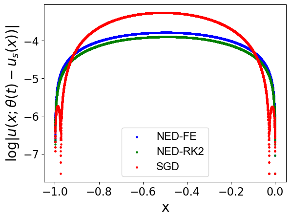
Performance lines. The numerical performance of NED will be shown as follows: the blue curve and its label "NED-FE" represent the explicit forward Euler method used in the NED method; the green curve and its label "NED-RK2" represent the 2nd order Runge-Kutta method used for solving NED flow; the red curve and its label "SGD" mean the stochastic gradient descent method.

5.1 Numerical Results of Evolution Equations for Supervised Learning

5.1.1 A One-Dimensional Example

We apply the NED method to solve the supervised learning problem (2.1) to approximate $y=sin(x)$ on $[0,D]$ .

Case 1: $D=2\pi$ . We train 200 epochs to compare our NED with SGD. The initial learning rate is $\tau_{0}=1.0e-03$ and the min-batch size is set to be 200. The gradient flow (4.4) for NED and the gradient flow (4.7) for SGD are used in the numerical comparison. We can see from Figure 2 (a) and (c) that 1) the NED methods with RK2 and FE solvers achieve better accuracy than the SGD method; 2) the NED with RK2 solver is more accurate than the NED with FE solver.

Case 2: $D=10\pi$ . We employ the activation function $\sigma=aReLU(x)+bsin(x)$ inspired by [41], where $a$ and $b$ are trainable parameters. The initial learning rate is $\tau_{0}=1.0e-3$ and the epoch size is 500. It can be seen from Figure 2 (b) and (d) that the NED methods with both FE and RK2 solvers are more accurate than the SGD method while the NED with RK2 solver is more accurate than the NED with FE solver.

5.1.2 A Multi-Dimensional Example

We test the NED method to approximate $y=\|\bm{x}\|_{2}^{2}$ on the domain $[-1,1]^{d}$ for $d=2$ , $d=10$ , and $d=30$ , where $\bm{x}=[x_{1},\cdots,x_{d}]$ . We apply an FNN with 1 hidden layer and a width of 50. The initial learning rate $\tau_{0}$ for the NED method is set as $3.0e-03$ with 2500 epochs. The initial learning rate for the SGD method is set as $1.0e-02$ . Each epoch of the training data has 2,000 random sample points on $[-1,1]^{d}$ . We can observe from Figure 3 that for $d=2$ , $d=10$ , and $d=30$ , the NED methods with different ODE solvers (FE and RK2) are much more accurate than the SGD method. We observe from Figure 3 that the green curve for NED-RK2 seems to overlap the blue curve for NED-FE for $d=2$ and $d=10$ . However, it should be pointed out that the NED with RK2 solver is a bit more accurate than the NED with FE solver for $d=2$ , $d=10$ , and $d=30$ .

5.2 Numerical Results of Evolution Equations for Solving PDEs

5.2.1 A One-Dimensional Nonlinear Boundary Value Problem

We consider the following nonlinear boundary value problem that seeks $u$ such that

\begin{split}&\partial_{t}u-\Delta u=-2u^{3},\text{in}\ [-1,0],\\ &u(-1)=\tfrac{1}{2},\qquad u(0)=\tfrac{1}{3}.\end{split}

(5.5)

It is obvious that the analytical steady state solution is $u_{s}(x)=\tfrac{1}{x+3}$ . Inspired by [25], we design a special network satisfying the boundary conditions automatically; i.e.,

u(x;\theta)=(x+1)(0-x)\hat{u}(x;\theta)+l_{1}(x),

where $l_{1}(x)=\tfrac{1}{2}+(\tfrac{1}{3}-\tfrac{1}{2})(x+1)$ and $\hat{u}(x;\theta)$ is the ResNet with two blocks of width 20. In each training iteration, we randomly select 10000 sample points in the interior domain $(-1,0)$ . The initial learning rate $\tau_{0}$ for the NED method is $3.0e-04$ with 3000 epochs. The initial learning rate for the SGD method is set as $5.0e-03$ . We can see from Figure 4 that our NED methods with ODE solvers (FE and RK2) trained by Algorithm 2 are more accurate than the SGD method when epoch $>1500$ .

5.2.2 A multi-dimension Linear Boundary Value Problem

We consider the heat equation that seeks $u$ such that

\left\{\begin{array}[]{lr}u_{t}-\Delta u=-d,&\text{in }\Omega=[0,1]^{d},\\ u(\bm{x},t)=\tfrac{1}{2}\|\bm{x}\|_{2}^{2},&\text{on }\partial\Omega.\\ \end{array}\right.

(5.6)

Obviously, the analytical steady state solution is $u_{s}(\bm{x})=\tfrac{1}{2}\|\bm{x}\|_{2}^{2}$ . We apply a special network structure automatically satisfying the boundary conditions introduced in [25]; i.e.,

u(\bm{x};\theta)=\prod_{i=1}^{d}(1-x_{i})x_{i}\hat{u}(\bm{x};\theta)+\ell_{1}(\bm{x}),

(5.7)

where $\hat{u}(\bm{x};\theta)$ is a neural network of three hidden layers and width 20, and

\ell_{1}(\bm{x})=\tfrac{1}{2}\|\bm{x}\|_{2}^{2}+\sin(2\pi\sum_{i=1}^{d}x_{i}){\displaystyle\prod_{i=1}^{d}x_{i}(1-x_{i})}.

We test the case of $d=5$ . Algorithm 2 is coupled with the forward Euler and the 2nd Runge-Kutta ODE solvers for the semi-discretization system. We randomly choose 10000 points in the interior of the domain. The initial learning rates for our NED method and the SGD method are $\tau_{0}=8.0e-3$ and $\tau_{0}=1.0e-1$ respectively. It can be seen from Figure 5 that 1) the NED methods with FE and RK2 solvers are more accurate than the SGD method in updating gradient flow to gain steady state solution $u_{s}(\bm{x};\infty)$ in the evolution equation; 2) our NED method with RK2 solver is a bit more accurate than our NED method with FE solver.

5.2.3 A multi-dimension Nonlinear Boundary Value Problem

We consider the following nonlinear boundary value problem that seeks $u$ such that

\left\{\begin{array}[]{lr}u_{t}-\Delta u+u^{3}-u=0,&\text{in }\Omega=[0,1]^{d},\\ u(\bm{x},t)=1,&\text{on}\ \partial\Omega.\\ \end{array}\right.

(5.8)

The analytical steady-state solution is $u_{s}(\bm{x})=1$ .We apply a special network structure automatically satisfying the boundary conditions introduced in [25]; i.e.,

u(\bm{x};\theta)=\prod_{i=1}^{d}(1-x_{i})x_{i}\hat{u}(\bm{x};\theta)+\ell_{1}(\bm{x}),

(5.9)

where $\hat{u}(\bm{x};\theta)$ is a neural network of three hidden layers and width 20, and

\ell_{1}(\bm{x})=1+\sin(2\pi\sum_{i=1}^{d}x_{i}){\displaystyle\prod_{i=1}^{d}x_{i}(1-x_{i})}.

We test the case for $d=5$ . We randomly choose 20000 points in the interior domain and employ Algorithm 2 coupled with the forward Euler and 2nd Runge-Kutta ODE solvers to solve the semi-discretization system. The initial learning rates for our NED method and the SGD method are $\tau_{0}=5.0e-7$ and $\tau_{0}=5.0e-1$ , respectively. Figure 6 shows 1) the numerical performance of our NED methods with FE and RK2 solvers is better than the SGD method; 2) our NED method with RK2 solver is more accurate than the NED method with FE solver.

6 Conclusion

In this paper, we propose a novel network-based optimization method called the Neural Energy Descent method (NED) to solve deep learning problems via identifying steady-state solutions of evolution equations. NED is powerful to be applied to a wide range of machine learning problems such as supervised learning and solving PDEs. We have developed a deep network approximation theory to justify the NED scheme. Numerical results have been observed to demonstrate the significant advantage of our NED method over the SGD method. In future work, we shall study the optimization convergence from the viewpoint of variational functional minimization and the generalization error of NED since random samples are used in the solver. This work will provide a complete theory of this new optimization algorithm for deep learning.

Acknowledgements

W. H. was supported by the National Science Foundation award DMS-2052685 and the National Institutes of Health award 1R35GM146894. C. W. was partially supported by National Science Foundation under awards DMS-2136380 and DMS-2206332. H. Y. was partially supported by the US National Science Foundation under awards DMS-2244988, DMS-2206333, and the Office of Naval Research Award N00014-23-1-2007.

References

[1] A. R. Barron. Universal approximation bounds for superpositions of a sigmoidal function. IEEE Trans. Inf. Theory, 39(3):930–945, 1993.
[2] J. Berg and K. Nyström. A Unified Deep Artificial Neural Network Approach to Partial Differential Equations in Complex Geometries. Neurocomputing, 317:28 – 41, 2018.
[3] J. Berner, P. Grohs, and A. Jentzen. Analysis of the generalization error: Empirical risk minimization over deep artificial neural networks overcomes the curse of dimensionality in the numerical approximation of black-scholes partial differential equations. SIAM Journal on Mathematics of Data Science, 2(3):631–657, 2020.
[4] S. Brenner and R. Scott. Polynomial Approximation Theory in Sobolev Spaces, pages 93–127. Springer New York, New York, NY, 2008.
[5] W. Cai, X. Li, and L. Liu. A phase shift deep neural network for high frequency approximation and wave problems. SIAM J. Sci. Comput., 42(5):A3285–A3312, 2020.
[6] W. Cai and Z. J. Xu. Multi-scale deep neural networks for solving high dimensional PDEs. arXiv e-prints, arXiv:1910.11710, 2019.
[7] Z. Cai, J. Chen, M. Liu, and X. Liu. Deep least-squares methods: An unsupervised learning-based numerical method for solving elliptic pdes. Journal of Computational Physics, page 109707, 2020.
[8] J. Chen, R. Du, P. Li, and L. Lyu. Quasi-monte carlo sampling for machine-learning partial differential equations. ArXiv, abs/1911.01612, 2019.
[9] Z. Chen, J. Lu, Y. Lu, and S. Zhou. A regularity theory for static schrödinger equations on $\mathbb{R}^{d}$ in spectral barron spaces. arxiv preprint arxiv:2201.10072, 2022.
[10] Z. Chen and H. Zhang. Learning implicit fields for generative shape modeling. In 2019 IEEE/CVF Conference on Computer Vision and Pattern Recognition (CVPR), pages 5939–5948, 2019.
[11] A. Chkifa, A. Cohen, and C. Schwab. Breaking the curse of dimensionality in sparse polynomial approximation of parametric pdes. Journal de Mathématiques Pures et Appliquées, 103(2):400 – 428, 2015.
[12] R. A. Devore, R. Howard, and C. Micchelli. Optimal nonlinear approximation. Manuskripta Math, pages 469–478, 1989.
[13] M. W. M. G. Dissanayake and N. Phan-Thien. Neural-network-based approximations for solving partial differential equations. Communications in Numerical Methods in Engineering, 10(3):195–201, 1994.
[14] W. E, C. Ma, and Q. Wang. A priori estimates of the population risk for residual networks. ArXiv, abs/1903.02154, 2019.
[15] W. E, C. Ma, and L. Wu. Barron Spaces and the Compositional Function Spaces for Neural Network Models. arXiv e-prints, arXiv:1906.08039, Jun 2019.
[16] W. E, C. Ma, and L. Wu. A priori estimates of the population risk for two-layer neural networks. Communications in Mathematical Sciences, 17(5):1407 – 1425, 2019.
[17] W. E and Q. Wang. Exponential convergence of the deep neural network approximation for analytic functions. Science China Mathmatics, 61(10):1733–1740, 2018.
[18] M. Ehrhardt and R. E. Mickens. A fast, stable and accurate numerical method for the Black-Scholes equation of American options. Int. J. Theor. Appl. Finance, 11(5):471–501, 2008.
[19] L. Evans and A. M. Society. Partial Differential Equations. Graduate studies in mathematics. American Mathematical Society, 1998.
[20] A. Gaikwad and I. M. Toke. Gpu based sparse grid technique for solving multidimensional options pricing pdes. In Proceedings of the 2Nd Workshop on High Performance Computational Finance, WHPCF ’09, pages 6:1–6:9, New York, NY, USA, 2009. ACM.
[21] K. Genova, F. Cole, A. Sud, A. Sarna, and T. Funkhouser. Local deep implicit functions for 3d shape. In 2020 IEEE/CVF Conference on Computer Vision and Pattern Recognition (CVPR), pages 4857–4866, 2020.
[22] D. Gobovic and M. E. Zaghloul. Analog cellular neural network with application to partial differential equations with variable mesh-size. In Proceedings of IEEE International Symposium on Circuits and Systems - ISCAS ’94, volume 6, pages 359–362 vol.6, May 1994.
[23] I. Goodfellow, Y. Bengio, and A. Courville. Deep Learning. MIT Press, Cambridge, 2016.
[24] P. Grisvard. Elliptic Problems in Nonsmooth Domains. Classics in Applied Mathematics. Society for Industrial and Applied Mathematics, 2011.
[25] Y. Gu, C. Wang, and H. Yang. Structure probing neural network deflation. Journal of Computational Physics, 434:110231, 2021.
[26] Y. Gu, H. Yang, and C. Zhou. SelectNet: Self-paced Learning for High-dimensional Partial Differential Equations. Journal of Computational Physics, 441:110444, 2021.
[27] I. Gühring, G. Kutyniok, and P. Petersen. Error bounds for approximations with deep relu neural networks in ws,p norms. Analysis and Applications, 18(05):803–859, 2020.
[28] J. Han, A. Jentzen, and W. E. Solving high-dimensional partial differential equations using deep learning. Proc. Natl. Acad. Sci., 115(34):8505–8510, 2018.
[29] J. Huang, H. Wang, and H. Yang. Int-deep: A deep learning initialized iterative method for nonlinear problems. Journal of Computational Physics, 419:109675, 2020.
[30] M. Hutzenthaler, A. Jentzen, T. Kruse, and T. A. Nguyen. A proof that rectified deep neural networks overcome the curse of dimensionality in the numerical approximation of semilinear heat equations. Partial Differ. Equ. Appl., 1(2):Paper No. 10, 34, 2020.
[31] M. Hutzenthaler, A. Jentzen, and P. von Wurstemberger. Overcoming the curse of dimensionality in the approximative pricing of financial derivatives with default risks. Electron. J. Probab., 25:Paper No. 101, 73, 2020.
[32] T. Jeruzalski, B. Deng, M. Norouzi, J. P. Lewis, G. Hinton, and A. Tagliasacchi. Nasa: Neural articulated shape approximation. Computer Vision–ECCV 2020:16th European Conference, Glasgow, UK, August 23–28,2020,Proceedings,Part VII 16, pages 612–628, 2020.
[33] Y. Jiao, Y. Lai, Y. Wang, H. Yang, and Y. Yang. Convergence analysis of the deep galerkin method for weak solutions. arXiv:2302.02405, 2023.
[34] S. Justin and S. Konstantinos. Dgm: A deep learning algorithm for solving partial differential equations. J. Comput. Phys., 375:1339–1364, 2018.
[35] A. Karpatne, G. Atluri, J. H. Faghmous, M. Steinbach, A. Banerjee, A. Ganguly, S. Shekhar, N. Samatova, and V. Kumar. Theory-guided data science: A new paradigm for scientific discovery from data. IEEE Transactions on Knowledge and Data Engineering, 29:2318–2331, 2017.
[36] Y. Khoo, J. Lu, and L. Ying. Solving parametric pde problems with artificial neural networks. European Journal of Applied Mathematics, 32(3):421–435, 2021.
[37] I. Lagaris, A. Likas, and D. I. Fotiadis. Artificial Neural Networks for Solving Ordinary and Partial Differential Equations. IEEE Trans. Neural Networks, 9:987–1000, 1998.
[38] I. E. Lagaris, A. Likas, and D. I. Fotiadis. Artificial neural networks for solving ordinary and partial differential equations. IEEE transactions on neural networks, 9(5):987–1000, 1998.
[39] H. Lee and I. S. Kang. Neural algorithm for solving differential equations. Journal of Computational Physics, 91(1):110 – 131, 1990.
[40] T. Lee, F. Wang, and R. Newell. Robust model-order reduction of complex biological processes. Journal of Process Control, 12(7):807 – 821, 2002.
[41] S. Liang, L. Lyu, C. Wang, and H. Yang. Reproducing activation function for deep learning. arXiv preprint arXiv:2101.04844, 2021.
[42] S. Liang and R. Srikant. Why deep neural networks for function approximation? In 5th International Conference on Learning Representations,ICLR 2017, 2017.
[43] S. Liu, Y. Zhang, S. Peng, B. Shi, M. Pollefeys, and Z. Cui. Dist: Rendering deep implicit signed distance function with differentiable sphere tracing. In 2020 IEEE/CVF Conference on Computer Vision and Pattern Recognition (CVPR), pages 2019–2028, 2020.
[44] Y. Liu, T. Gao, and H. Yang. SelectNet: Learning to sample from the wild for imbalanced data training. In J. Lu and R. Ward, editors, Proceedings of The First Mathematical and Scientific Machine Learning Conference, volume 107 of Proceedings of Machine Learning Research, pages 193–206. PMLR, 20–24 Jul 2020.
[45] Z. Liu, W. Cai, and Z.-Q. J. Xu. Multi-scale deep neural network (mscalednn) for solving poisson-boltzmann equation in complex domains. Communications in Computational Physics, 28(5):1970–2001, Jun 2020.
[46] J. Lu and Y. Lu. A priori generalization error analysis of two-layer neural networks for solving high dimensional schrödinger eigenvalue problems. Communications of the American Mathematical Soceity, 2(01), 2022.
[47] J. Lu, Z. Shen, H. Yang, and S. Zhang. Deep network approximation for smooth functions. SIAM Journal on Mathematical Analysis, 53(5):5465–5506, 2021.
[48] T. Luo and H. Yang. Two-Layer Neural Networks for Partial Differential Equations: Optimization and Generalization Theory. arXiv e-prints, arXiv:2006.15733, 2020.
[49] L. Lyu, K. Wu, R. Du, and J. Chen. Enforcing exact boundary and initial conditions in the deep mixed residual method. arXiv preprint arXiv:2008.01491, 2020.
[50] M. Michalkiewicz, J. K. Pontes, D. Jack, M. Baktashmotlagh, and A. Eriksson. Implicit surface representations as layers in neural networks. In 2019 IEEE/CVF International Conference on Computer Vision (ICCV), pages 4742–4751, 2019.
[51] H. Montanelli and Q. Du. New error bounds for deep relu networks using sparse grids. SIAM Journal on Mathematics of Data Science, 1(1):78–92, 2019.
[52] H. Montanelli and H. Yang. Error bounds for deep relu networks using the kolmogorov–arnold superposition theorem. Neural Networks, 129:1–6, 2020.
[53] H. Montanelli, H. Yang, and Q. Du. Deep relu networks overcome the curse of dimensionality for bandlimited functions. Journal of Computational Mathematics, 39(6), 2021.
[54] T. Nakamura-Zimmerer, Q. Gong, and W. Kang. Adaptive deep learning for high dimensional hamilton-jacobi-bellman equations. SIAM Journal on Scientific Computing, 43(2):A1221–A1247, 2021.
[55] J. A. A. Opschoor, C. Schwab, and J. Zech. Exponential relu dnn expression of holomorphic maps in high dimension. Constructive Approximation, 55(1):537–582, 2022.
[56] Owens and Filkin. Efficient training of the backpropagation network by solving a system of stiff ordinary differential equations. In International 1989 Joint Conference on Neural Networks, pages 381–386 vol.2, 1989.
[57] S. Pan and K. Duraisamy. Physics-informed probabilistic learning of linear embeddings of nonlinear dynamics with guaranteed stability. SIAM Journal on Applied Dynamical Systems, 19:480–509, 2020.
[58] J. J. Park, P. Florence, J. Straub, R. Newcombe, and S. Lovegrove. Deepsdf: Learning continuous signed distance functions for shape representation. In 2019 IEEE/CVF Conference on Computer Vision and Pattern Recognition (CVPR), pages 165–174, 2019.
[59] T. Poggio, H. Mhaskar, L. Rosasco, B. Miranda, and Q. Liao. Why and when can deep—but not shallow—networks avoid the curse of dimensionality: A review. International Journal of Automation and Computing, 14:503–519, 2017.
[60] M. Raissi, P. Perdikaris, and G. Karniadakis. Physics-informed neural networks: A deep learning framework for solving forward and inverse problems involving nonlinear partial differential equations. Journal of Computational Physics, 378:686 – 707, 2019.
[61] S. Saito, Z. Huang, R. Natsume, S. Morishima, A. Kanazawa, and H. Li. Pifu: Pixel-aligned implicit function for high-resolution clothed human digitization. 2019 IEEE/CVF International Conference on Computer Vision (ICCV), pages 2304–2314, 2019.
[62] Z. Shen, H. Yang, and S. Zhang. Deep network approximation characterized by number of neurons. Communications in Computational Physics, 28(5), 2019.
[63] Z. Shen, H. Yang, and S. Zhang. Nonlinear approximation via compositions. Neural Networks, 119:74 – 84, 2019.
[64] Z. Shen, H. Yang, and S. Zhang. Deep network with approximation error being reciprocal of width to power of square root of depth. Neural Comput., 33(4):1005–1036, 2021.
[65] Z. Shen, H. Yang, and S. Zhang. Neural network approximation: Three hidden layers are enough. Neural Networks, 141:160–173, 2021.
[66] Y. Shin, J. Darbon, and G. Karniadakis. On the convergence and generalization of physics informed neural networks. ArXiv, abs/2004.01806, 2020.
[67] J. W. Siegel and J. Xu. Approximation rates for neural networks with general activation functions. Neural Networks, 128:313–321, 2020.
[68] V. Sitzmann, M. Zollhöfer, and G. Wetzstein. Scene representation networks: Continuous 3d-structure-aware neural scene representations. Advances in Neural Information Processing Systems, 32, 2019.
[69] E. M. STEIN. Singular Integrals and Differentiability Properties of Functions (PMS-30). Princeton University Press, 1970.
[70] M. Tancik, P. P. Srinivasan, B. Mildenhall, S. Fridovich-Keil, N. Raghavan, U. Singhal, R. Ramamoorthi, J. T. Barron, and R. Ng. Fourier features let networks learn high frequency functions in low dimensional domains. Advances in Neural Information Processing Systems, 33:7537–7547, 2020.
[71] D. J. Wales and J. P. K. Doye. Stationary points and dynamics in high-dimensional systems. The Journal of chemical physics, 119(23):12409–12416, 2003.
[72] Z.-Q. J. Xu, Y. Zhang, T. Luo, Y. Xiao, and Z. Ma. Frequency principle: Fourier analysis sheds light on deep neural networks. Communications in Computational Physics, 28(5):1746–1767, 2020.
[73] D. Yarotsky. Error bounds for approximations with deep ReLU networks. Neural Networks, 94:103 – 114, 2017.
[74] D. Yarotsky. Optimal approximation of continuous functions by very deep ReLU networks. In S. Bubeck, V. Perchet, and P. Rigollet, editors, Proceedings of the 31st Conference On Learning Theory, volume 75 of Proceedings of Machine Learning Research, pages 639–649. PMLR, 06–09 Jul 2018.
[75] D. Yarotsky and A. Zhevnerchuk. The phase diagram of approximation rates for deep neural networks. Advances in neural information processing systems, 33:13005–13015, 2020.
[76] H. Yserentant. Sparse grid spaces for the numerical solution of the electronic Schrödinger equation. Numer. Math., 101(2):381–389, 2005.
[77] Y. A. Yucesan and F. A. C. Viana. A physics-informed neural network for wind turbine main bearing fatigue. International Journal of Prognostics and Health Management, 11, 2020.
[78] Y. Zang, G. Bao, X. Ye, and H. Zhou. Weak adversarial networks for high-dimensional partial differential equations. J. Comput. Phys., 411:109409, 2020.

Appendix A Notations and Definitions

We first introduce notations and definitions throughout this paper.

A.1 Deep Neural Networks

Let us summarize all basic notations used in deep neural networks as follows.

•

Matrices are denoted by bold uppercase letters. For instance, $\bm{A}\in\mathbb{R}^{m\times n}$ is a real matrix of size $m\times n$ , and $\bm{A}^{T}$ denotes the transpose of $\bm{A}$ .
•

Vectors are denoted as bold lowercase letters. For example, $\bm{v}\in{\mathbb{R}}^{n}$ is a column vector of size $n$ . Correspondingly, $\bm{v}(i)$ is the $i$ -th element of $\bm{v}$ . $\bm{v}=[v_{1},\cdots,v_{n}]^{T}=\left[\hskip-4.0pt\begin{array}[]{c}\vskip-3.0ptv_{1}\\ \vskip-5.0pt\vdots\\ v_{n}\end{array}\hskip-4.0pt\right]$ is a vector with $\bm{v}(i)=v_{i}$ .
•
A $d$ -dimensional multi-index is a $d$ -tuple ${\bm{\alpha}}=[\alpha_{1},\alpha_{2},\cdots,\alpha_{d}]^{T}\in\mathbb{N}^{d}.$ Several related notations are listed below.
- –
  
  $|{\bm{\alpha}}|=|\alpha_{1}|+|\alpha_{2}|+\cdots+|\alpha_{d}|$ ;
- –
  
  ${\bm{x}}^{\bm{\alpha}}=x_{1}^{\alpha_{1}}x_{2}^{\alpha_{2}}\cdots x_{d}^{\alpha_{d}}$ , where ${\bm{x}}=[x_{1},x_{2},\cdots,x_{d}]^{T}$ ;
- –
  
  ${\bm{\alpha}}!=\alpha_{1}!\alpha_{2}!\cdots\alpha_{d}!$ .
•

Let $B_{r,|\cdot|}({\bm{x}})\subseteq{\mathbb{R}}^{d}$ be the closed ball with a center ${\bm{x}}\subseteq{\mathbb{R}}^{d}$ and a radius $r$ measured by the Euclidean distance. Similarly, $B_{r,\|\cdot\|_{\ell^{\infty}}}({\bm{x}})\subseteq{\mathbb{R}}^{d}$ is a ball measured by the discrete $\ell^{\infty}$ -norm of a vector.
•

Assume $\bm{n}\in\mathbb{N}^{n}$ , then $f(\bm{n})=\mathcal{O}(g(\bm{n}))$ means that there exists positive $C$ independent of $\bm{n}$ , $f$ , and $g$ such that $f(\bm{n})\leq Cg(\bm{n})$ when all entries of $\bm{n}$ go to $+\infty$ .
•

We will use $\sigma$ to denote activation functions. Let $\sigma_{1}:{\mathbb{R}}\to{\mathbb{R}}$ denote the rectified linear unit (ReLU), i.e. $\sigma_{1}(x)=\max\{0,x\}$ . With the abuse of notations, we define $\sigma_{1}:{\mathbb{R}}^{d}\to{\mathbb{R}}^{d}$ as $\sigma_{1}({\bm{x}})=\left[\begin{array}[]{c}\max\{0,x_{1}\}\\ \vdots\\ \max\{0,x_{d}\}\end{array}\right]$ for any ${\bm{x}}=[x_{1},\cdots,x_{d}]^{T}\in{\mathbb{R}}^{d}$ . Furthermore, let $\sigma_{2}:{\mathbb{R}}\to{\mathbb{R}}$ be $\sigma_{1}^{2}$ and similarly we define the action of $\sigma_{2}$ on a vector ${\bm{x}}$ .
•
We will use NN as a neural network for short and $\sigma_{r}$ -NN to specify an NN with activation functions $\sigma_{t}$ with $t\leq r$ . We will also use Python-type notations to specify a class of NNs, e.g., $\sigma_{1}$ - $\textnormal{NN}(\textnormal{c}_{1};\ \textnormal{c}_{2};\ \cdots;\ \textnormal{c}_{m})$ is a set of ReLU FNNs satisfying $m$ conditions given by $\{\textnormal{c}_{i}\}_{1\leq i\leq m}$ , each of which may specify the number of inputs (#input), the total number of nodes in all hidden layers ( $\#$ node), the number of hidden layers ( $\#$ layer), the number of total parameters ( $\#$ parameter), and the width in each hidden layer (widthvec), the maximum width of all hidden layers (maxwidth), etc. For example, if $\phi\in\sigma_{1}$ - $\textnormal{NN}(\textnormal{\#input}=2;\,\textnormal{widthvec}=[100,100])$ , then $\phi$ satisfies
- –
  
  $\phi$ maps from ${\mathbb{R}}^{2}$ to ${\mathbb{R}}$ .
- –
  
  $\phi$ has two hidden layers and the number of nodes in each hidden layer is $100$ .

•

$[n]^{L}$ is short for $[n,n,\cdots,n]\in\mathbb{N}^{L}$ . For example,

\textnormal{NN}(\textnormal{\#input}=d;\,\textnormal{widthvec}=[100,100])=\textnormal{NN}(\textnormal{\#input}=d;\,\textnormal{widthvec}=[100]^{2}).

•

For $\phi\in\textnormal{NN}(\textnormal{\#input}=d;\,\textnormal{widthvec}=[N_{1},N_{2},\cdots,N_{L}])$ , if we define $N_{0}=d$ and $N_{L+1}=1$ , then the architecture of $\phi$ can be briefly described as follows:

\displaystyle\bm{x}=\tilde{\bm{h}}_{0}\mathop{\raisebox{0.0pt}{\scalebox{2.6}[1]{$\longrightarrow$}}}^{\bm{W}_{1},\ \bm{b}_{1}}\bm{h}_{1}\mathop{\longrightarrow}^{\sigma}\tilde{\bm{h}}_{1}\cdots\mathop{\raisebox{0.0pt}{\scalebox{2.6}[1]{$\longrightarrow$}}}^{\bm{W}_{L},\ \bm{b}_{L}}\bm{h}_{L}\mathop{\longrightarrow}^{\sigma}\tilde{\bm{h}}_{L}\mathop{\mathop{\raisebox{0.0pt}{\scalebox{2.6}[1]{$\longrightarrow$}}}}^{\bm{W}_{L+1},\ \bm{b}_{L+1}}\phi(\bm{x})=\bm{h}_{L+1},

where $\bm{W}_{i}\in{\mathbb{R}}^{N_{i}\times N_{i-1}}$ and $\bm{b}_{i}\in{\mathbb{R}}^{N_{i}}$ are the weight matrix and the bias vector in the $i$ -th linear transform in $\phi$ , respectively, i.e.,

\bm{h}_{i}:=\bm{W}_{i}\tilde{\bm{h}}_{i-1}+\bm{b}_{i},\quad\textnormal{for $i=1$, $\dots$, $L+1$,}

and

\tilde{\bm{h}}_{i}=\sigma(\bm{h}_{i}),\quad\textnormal{for $i=1$, $\dots$, $L$.}

$L$ in this paper is also called the number of hidden layers in the literature.

•
The expression, an FNN with width $N$ and depth $L$ , means
- –
  
  The maximum width of this FNN for all hidden layers less than or equal to $N$ .
- –
  
  The number of hidden layers of this FNN less than or equal to $L$ .

Lemma A.1.

A list of examples and basic lemmas of $\sigma_{1}$ -NNs.

(i)

Any one-dimensional continuous piecewise linear function with $N$ breakpoints can be exactly realized by a one-hidden layer $\sigma_{1}$ -NN with $N$ neurons in the hidden layer.
(ii)

Any identity map in ${\mathbb{R}}^{d}$ can be carried out precisely by a $\sigma_{1}$ -NN with one hidden layer and $2d$ neurons.
(iii)

(Lemma 5.1 of [47]) For any $N,L\in\mathbb{N}^{+}$ , there exists a $\sigma_{1}$ -NN $\phi$ with width $3N$ and depth $L$ such that

$|\phi(x)-x^{2}|\leq N^{-L},\quad\forall x\in[0,1].$
(iv)

(Lemma 4.2 of [47]) For any $N,L\in\mathbb{N}^{+}$ and $a,b\in{\mathbb{R}}$ with $a<b$ , there exists a $\sigma_{1}$ -NN $\phi$ with width $9N+1$ and depth $L$ such that

$|\phi(x,y)-xy|\leq 6(b-a)^{2}N^{-L},\quad\forall x,y\in[a,b].$
(v)

(Proposition 4.1 of [47]) Assume $P({\bm{x}})={\bm{x}}^{\bm{\alpha}}=x_{1}^{\alpha_{1}}x_{2}^{\alpha_{2}}\cdots x_{d}^{\alpha_{d}}$ for ${\bm{\alpha}}\in\mathbb{N}^{d}$ with $|{\bm{\alpha}}|=k\geq 2$ . For any $N,L\in\mathbb{N}^{+}$ , there exists a $\sigma_{1}$ -NN $\phi$ with width $9(N+1)+k-2$ and depth $7k(k-1)L$ such that

$|\phi({\bm{x}})-P({\bm{x}})|\leq 9(k-1)(N+1)^{-7kL},\quad\forall{\bm{x}}\in[0,1]^{d}.$
(vi)

Assume $P({\bm{x}})=\sum_{j=1}^{J}c_{j}{\bm{x}}^{{\bm{\alpha}}_{j}}$ for ${\bm{\alpha}}_{j}\in\mathbb{N}^{d}$ with $k=\max_{j}|{\bm{\alpha}}_{j}|\geq 2$ . For any $N,L\in\mathbb{N}^{+}$ , there exists a $\sigma_{1}$ -NN $\phi$ with width $(9(N+1)+k-2)J$ and depth $7k(k-1)L$ such that

$|\phi({\bm{x}})-P({\bm{x}})|\leq 9J(k-1)(N+1)^{-14L},\quad\forall{\bm{x}}\in[0,1]^{d}.$
(vii)

Assume $P({\bm{x}})=\min\{x_{1},x_{2},\dots,x_{n}\}$ for ${\bm{x}}\in{\mathbb{R}}^{n}$ , there exists a $\sigma_{1}$ -NN $\phi({\bm{x}})$ of width $2n$ and depth $n-1$ such that $\phi({\bm{x}})=P({\bm{x}})$ for any ${\bm{x}}\in{\mathbb{R}}^{n}$ .

Proof.

(i) and (ii) are simple. (iii) to (v) are quoted from [47].

Part (vi): In the case of $\min_{j}|{\bm{\alpha}}_{j}|\geq 2$ , the $\sigma_{1}$ -NN in (vi) can be constructed by stacking $J$ $\sigma_{1}$ -NNs approximating ${\bm{x}}^{{\bm{\alpha}}_{j}}$ by (vi). In the case when $|{\bm{\alpha}}_{j}|\leq 1$ for some $j$ ’s, these terms can be easily taken care of using the identity map in (ii).

Part (vii): The proof of (vii) is based on the observation that $\min\{x,y\}=\tfrac{x+y-|x-y|}{2}$ , which can be represented exactly with a $\sigma_{1}$ -NN of width $4$ and depth $1$ . We can repeatedly apply this observation to build the desired network that evaluates a $\min$ operator of two numbers per hidden layer. Each $\min$ operator takes $4$ neurons per layer and extra $2(n-2)$ neurons per layer are required to generate an identify map of dimension at least $n-2$ to pass unused numbers in ${\bm{x}}$ to the next layer. Hence, the total width requirement is $4+2(n-2)=2n$ and the depth requirement is $n-1$ . ∎

Lemma A.2.

A list of examples and basic lemmas of $\sigma_{2}$ -NNs.

(i)

$\sigma_{1}$ -NNs are $\sigma_{2}$ -NNs.
(ii)

Any identity map in ${\mathbb{R}}^{d}$ can be carried out precisely by a $\sigma_{2}$ -NN with one hidden layer and $2d$ neurons.
(iii)

$f(x)=x^{2}$ can be implemented via a one-hidden-layer $\sigma_{2}$ -NN with two neurons.
(iv)

$f(x,y)=xy=\tfrac{(x+y)^{2}-(x-y)^{2}}{4}$ can be implemented via a one-hidden-layer $\sigma_{2}$ -NN with four neurons.
(v)

Assume $P({\bm{x}})={\bm{x}}^{\bm{\alpha}}=x_{1}^{\alpha_{1}}x_{2}^{\alpha_{2}}\cdots x_{d}^{\alpha_{d}}$ for ${\bm{\alpha}}\in\mathbb{N}^{d}$ . For any $N,L\in\mathbb{N}^{+}$ such that $NL+2^{\lfloor\log_{2}N\rfloor}\geq|{\bm{\alpha}}|$ , there exists a $\sigma_{2}$ -NN $\phi$ with width $4N+2d$ and depth $L+\lceil\log_{2}N\rceil$ such that

$\phi({\bm{x}})=P({\bm{x}})\quad\textnormal{for any ${\bm{x}}\in{\mathbb{R}}^{d}$.}$
(vi)

Assume $P({\bm{x}})=\sum_{j=1}^{J}c_{j}{\bm{x}}^{{\bm{\alpha}}_{j}}$ for ${\bm{\alpha}}_{j}\in\mathbb{N}^{d}$ . For any $N,L,a,b\in\mathbb{N}^{+}$ such that $ab\geq J$ and $(L-2b-b\log_{2}N)N\geq b\max_{j}|{\bm{\alpha}}_{j}|$ , there exists a $\sigma_{2}$ -NN $\phi$ with width $4Na+2d+2$ and depth $L$ such that

$\phi({\bm{x}})=P({\bm{x}})\quad\textnormal{for any ${\bm{x}}\in{\mathbb{R}}^{d}$.}$

Proof.

(i) to (iv) are trivial. We will only prove (v) and (vi).

Part (v): In the case of $|{\bm{\alpha}}|=k\leq 1$ , the proof is simple and left for the reader. When $|{\bm{\alpha}}|=k\geq 2$ , the main idea of the proof of (v) can be summarized in Figure 7. We apply $\sigma_{1}$ -NNs to implement a $d$ -dimensional identity map as in Lemma A.1 (iii). These identity maps maintain necessary entries of ${\bm{x}}$ to be multiplied together. We apply $\sigma_{2}$ -NNs to implement the multiplication function in Lemma A.2 (iii) and carry out the multiplication $N$ times per layer. After $L$ layers, there are $k-NL\leq N$ multiplication to be implemented. Finally, these at most $N$ multiplications can be carried out with a small $\sigma_{2}$ -NNs in a dyadic tree structure.

Part (vi): The main idea of the proof is to apply Part (v) $J$ times to construct $J$ $\sigma_{2}$ -NNs, $\{\phi_{j}({\bm{x}})\}_{j=1}^{J}$ , to represent ${\bm{x}}^{{\bm{\alpha}}_{j}}$ and arrange these $\sigma_{2}$ -NNs as sub-NN blocks to form a larger $\sigma_{2}$ -NN $\tilde{\phi}({\bm{x}})$ with $ab$ blocks as shown in Figure 8, where each red rectangle represents one $\sigma_{2}$ -NN $\phi_{j}({\bm{x}})$ and each blue rectangle represents one $\sigma_{1}$ -NN of width $2$ as an identity map of ${\mathbb{R}}$ . There are $ab$ red blocks with $a$ rows and $b$ columns. When $ab\geq J$ , these sub-NN blocks can carry out all monomials ${\bm{x}}^{{\bm{\alpha}}_{j}}$ . In each column, the results of the multiplications of ${\bm{x}}^{{\bm{\alpha}}_{j}}$ are added up to the input of the narrow $\sigma_{1}$ -NN, which can carry the sum over to the next column. After the calculation of $b$ columns, $J$ additions of the monomials ${\bm{x}}^{{\bm{\alpha}}_{j}}$ have been implemented, resulting in the output $P({\bm{x}})$ .

By Part (v), for any $N\in\mathbb{N}^{+}$ , there exists a $\sigma_{2}$ -NN $\phi_{j}({\bm{x}})$ of width $2d+4N$ and depth $L_{j}=\lceil\tfrac{|{\bm{\alpha}}_{j}|}{N}\rceil+\lceil\log_{2}N\rceil$ to implement ${\bm{x}}^{{\bm{\alpha}}_{j}}$ . Note that $b\max_{j}L_{j}\leq b\left(\tfrac{\max_{j}|{\bm{\alpha}}_{j}|}{N}+2+\log_{2}N\right)$ . Hence, there exists a $\sigma_{2}$ -NN $\tilde{\phi}({\bm{x}})$ of width $2da+4Na+2$ and depth $b\left(\tfrac{\max_{j}|{\bm{\alpha}}_{j}|}{N}+2+\log_{2}N\right)$ to implement $P({\bm{x}})$ as in Figure 8. Note that the total width of each column of blocks is $2ad+4Na+2$ but in fact this width can be reduced to $2d+4Na+2$ , since the red blocks in each column can share the same identity map of ${\mathbb{R}}^{d}$ (the blue part of Figure 7).

Note that $b\left(\tfrac{\max_{j}|{\bm{\alpha}}_{j}|}{N}+2+\log_{2}N\right)\leq L$ is equivalent to $(L-2b-b\log_{2}N)N\geq b\max_{j}|{\bm{\alpha}}_{j}|$ . Hence, for any $N,L,a,b\in\mathbb{N}^{+}$ such that $ab\geq J$ and $(L-2b-b\log_{2}N)N\geq b\max_{j}|{\bm{\alpha}}_{j}|$ , there exists a $\sigma_{2}$ -NN $\phi({\bm{x}})$ with width $4Na+2d+2$ and depth $L$ such that $\tilde{\phi}({\bm{x}})$ is a sub-NN of $\phi({\bm{x}})$ in the sense of $\phi({\bm{x}})=\textnormal{Id}\circ\tilde{\phi}({\bm{x}})$ with Id as an identify map of ${\mathbb{R}}$ , which means that $\phi({\bm{x}})=\tilde{\phi}({\bm{x}})=P({\bm{x}})$ . The proof of Part (vi) is completed. ∎

We would like to remark that it is interesting to further optimize the above lemmas so that we can optimize the approximation theories in this paper. This is left as future work.

A.2 Sobolev spaces

We will use $D$ to denote the weak derivative of a single variable function and $D^{\bm{\alpha}}$ to denote the partial derivative $D^{\alpha_{1}}_{1}D^{\alpha_{2}}_{2}\dots D^{\alpha_{d}}_{d}$ of a $d$ -dimensional function with $\alpha_{i}$ as the order of derivative $D_{i}$ in the $i$ -th variable and ${\bm{\alpha}}=[\alpha_{1},\dots,\alpha_{d}]^{T}$ . Let $\Omega$ denote an open subset of $\mathbb{R}^{d}$ and $L^{p}(\Omega)$ be the standard Lebesgue space on $\Omega$ for $p\in[1,\infty]$ . We write $\nabla f:=[D_{1}f,\dots,D_{d}f]^{T}$ . $\partial\Omega$ is the boundary of $\Omega$ . Let $\mu(\cdot)$ be the Lebesgue measure. For $f(x)\in\mathcal{W}^{n,p}(\Omega)$ , we use the notation

\|f\|_{\mathcal{W}^{n,p}(\Omega)}=\|f\|_{\mathcal{W}^{n,p}}=\|f(x)\|_{\mathcal{W}^{n,p}(\Omega,\mu)},

if the domain is clear from the context and we use the Lebesgue measure. If ${\varrho}$ is a probability density function supported in $\Omega$ with $\mu_{\varrho}(\cdot)$ as its corresponding measure, then we use $\|f\|_{\mathcal{W}^{n,p}(\Omega,\mu_{\varrho})}$ to specify the measure in the Sobolev norm.

Definition A.3.

(Sobolev Space) Let $n\in\mathbb{N}_{0}$ and $1\leq p\leq\infty$ . Then we define the Sobolev space

\mathcal{W}^{n,p}(\Omega):=\{f\in L^{p}(\Omega):D^{\bm{\alpha}}f\in L^{p}(\Omega)\text{ for all }{\bm{\alpha}}\in\mathbb{N}_{0}^{d}\text{ with }|{\bm{\alpha}}|\leq n\}

with a norm

\|f\|_{\mathcal{W}^{n,p}(\Omega)}:=\left(\sum_{0\leq|{\bm{\alpha}}|\leq n}\|D^{\bm{\alpha}}f\|^{p}_{L^{p}(\Omega)}\right)^{1/p}

and

\|f\|_{\mathcal{W}^{n,\infty}(\Omega)}:=\max_{0\leq|{\bm{\alpha}}|\leq n}\|D^{\bm{\alpha}}f\|_{L^{\infty}(\Omega)}.

Many results of function approximation rely on the domain $\Omega$ and we will use the following condition on $\Omega$ (see [19], Appendix C.1).

Definition A.4.

(Lipschitz-domain) We say that a bounded and open set $\Omega\subseteq\mathbb{R}^{d}$ is a Lipschitz-domain if for each ${\bm{x}}_{0}\in\partial\Omega$ there exists $r>0$ and a Lipschitz continuous function $g:\mathbb{R}^{d-1}\rightarrow\mathbb{R}$ such that

\Omega\cap B_{r,|\cdot|}({\bm{x}}_{0})=\{{\bm{x}}\in B_{r,|\cdot|}({\bm{x}}):x_{d}>g(x_{1},\dots,x_{d-1})\},

after possibly relabeling and reordering the coordinate axes, where $B_{r,|\cdot|}({\bm{x}})$ is a sphere centered at ${\bm{x}}$ with a radius $r$ .

In this paper, we focus on an open, bounded, and convex domain $\Omega=(0,1)^{d}$ , which is a Lipschitz domain (see [24], Corollary 1.2.2.3).

Let us introduce some basic lemmas of Sobolev spaces here.

Lemma A.5.

Let $f$ be any $\sigma_{1}$ -NN and $g\in\mathcal{W}^{n,p}(\Omega)$ with $1\leq p\leq\infty$ , then $fg\in\mathcal{W}^{n,p}(\Omega)$ and there exists a constant $C=C(d,n,p)>0$ such that

|fg|_{\mathcal{W}^{n,p}(\Omega)}\leq C\left(|f|_{\mathcal{W}^{1,\infty}(\Omega)}|g|_{\mathcal{W}^{n-1,p}(\Omega)}+\|f\|_{L^{\infty}(\Omega)}|g|_{\mathcal{W}^{n,p}(\Omega)}\right).

For $p=\infty$ , we have $C=1$ .

Proof.

In the following proof, we will drop the dependence of the bounded domain $\Omega$ in all norms. Note that any $\sigma_{1}$ -NN is a piecewise linear function and hence $D^{\bm{\alpha}}f=0$ if $\alpha_{i}\geq 2$ for some $i\in\{1,\dots,d\}$ . Hence, $f\in\mathcal{W}^{n,\infty}$ for any $n\in\mathbb{N}$ . Note that $D^{\bm{\alpha}}(fg)=\sum_{{\bm{\alpha}}_{1}+{\bm{\alpha}}_{2}={\bm{\alpha}}}c_{{\bm{\alpha}}_{1},{\bm{\alpha}}_{2}}D^{{\bm{\alpha}}_{1}}gD^{{\bm{\alpha}}_{2}}f$ with constant coefficients $\{c_{{\bm{\alpha}}_{1},{\bm{\alpha}}_{2}}\}$ . By the triangle inequality and the inequalities

\left(\sum_{i=1}^{n}a_{i}^{p}\right)^{1/p}\leq\sum_{i=1}^{n}a_{i}\leq c_{1}(n,p)\left(\sum_{i=1}^{n}a_{i}^{p}\right)^{1/p}

for $a_{i}\geq 0$ and some $c_{1}(n,p)>0$ , it is also easy to check that there exist a constant $c_{2}(d,n,p)$ such that

|fg|_{\mathcal{W}^{n,p}}\leq\|fg\|_{\mathcal{W}^{n,p}}\leq c_{2}(d,n,p)\|f\|_{\mathcal{W}^{n,\infty}}\|g\|_{\mathcal{W}^{n,p}}.

Hence, $fg\in\mathcal{W}^{n,p}$ . In the above inequality, $\|f\|_{\mathcal{W}^{n,\infty}}$ can be replaced with $\|f\|_{\mathcal{W}^{d,\infty}}$ if $n\geq d$ because $f$ is a $\sigma_{1}$ -NN.

By the same inequalities, we can verify that

$\displaystyle\|fg\|_{\mathcal{W}^{n,p}(\Omega)}$	$\displaystyle=$	$\displaystyle\left(\sum_{\|{\bm{\alpha}}\|=n}\\|\sum_{{\bm{\alpha}}_{1}+{\bm{\alpha}}_{2}={\bm{\alpha}}}c_{{\bm{\alpha}}_{1},{\bm{\alpha}}_{2}}D^{{\bm{\alpha}}_{1}}gD^{{\bm{\alpha}}_{2}}f\\|_{L^{p}}^{p}\right)^{1/p}$
	$\displaystyle\leq$	$\displaystyle\sum_{\|{\bm{\alpha}}\|=n}\\|\sum_{{\bm{\alpha}}_{1}+{\bm{\alpha}}_{2}={\bm{\alpha}}}c_{{\bm{\alpha}}_{1},{\bm{\alpha}}_{2}}D^{{\bm{\alpha}}_{1}}gD^{{\bm{\alpha}}_{2}}f\\|_{L^{p}}$
	$\displaystyle\leq$	$\displaystyle\sum_{\|{\bm{\alpha}}\|=n}\sum_{{\bm{\alpha}}_{1}+{\bm{\alpha}}_{2}={\bm{\alpha}}}\|c_{{\bm{\alpha}}_{1},{\bm{\alpha}}_{2}}\|\\|D^{{\bm{\alpha}}_{1}}gD^{{\bm{\alpha}}_{2}}f\\|_{L^{p}}$
	$\displaystyle\leq$	$\displaystyle c_{3}(d,n)\sum_{\|{\bm{\alpha}}_{1}+{\bm{\alpha}}_{2}\|=n}\\|D^{{\bm{\alpha}}_{1}}gD^{{\bm{\alpha}}_{2}}f\\|_{L^{p}}$
	$\displaystyle\leq$	$\displaystyle c_{3}(d,n)\sum_{\|{\bm{\alpha}}_{1}+{\bm{\alpha}}_{2}\|=n,\\|{\bm{\alpha}}_{2}\\|_{\ell^{\infty}}=1}\\|D^{{\bm{\alpha}}_{1}}gD^{{\bm{\alpha}}_{2}}f\\|_{L^{p}}$
		$\displaystyle+c_{3}(d,n)\sum_{\|{\bm{\alpha}}_{1}\|=n}\\|D^{{\bm{\alpha}}_{1}}gf\\|_{L^{p}}$
	$\displaystyle\leq$	$\displaystyle C(d,n,p)\left(\|f\|_{\mathcal{W}^{1,\infty}(\Omega)}\|g\|_{\mathcal{W}^{n-1,p}(\Omega)}+\\|f\\|_{L^{\infty}(\Omega)}\|g\|_{\mathcal{W}^{n,p}(\Omega)}\right).$

The case of $p=\infty$ is simple. ∎

Appendix B Deep Network Approximation in the Sobolev Space

We prove the basic theories of Deep Network Approximation for parametrized functions in the Sobolev Space $\mathcal{W}^{n,p}$ for $\sigma_{1}$ -NNs and $\sigma_{2}$ -NNs. The proofs of the theories developed here mainly follow previous works in [63, 62, 47, 27, 55]. The focus of [63, 62, 47] is on the optimal approximation rate of deep networks in terms of width $N$ and depth $L$ for continuous and $C^{m}$ functions, while [27, 55] describe the approximation rate in terms of the number of parameters $W$ in deep networks for $\mathcal{W}^{n,p}$ (with $n\in[0,1]$ and $p\in[1,\infty]$ ) and $\mathcal{W}^{n,\infty}$ (for any $n\in\mathbb{N}$ ), respectively. We aim at characterizing deep network approximation for solution manifolds of parametric PDEs depending on $d_{t}$ -dimensional parameters $t\in{\mathbb{R}}^{d_{t}}$ . We focus on the case when the solutions $u({\bm{x}},t)$ of PDEs are in the space $\mathcal{W}^{n,p}\times C^{m}$ . The theories developed here are new and are motivated by the NED method, where we consider the semi-discretization of $u({\bm{x}},t)$ via a neural network $U({\bm{x}};{\bm{\theta}}(t))$ , in which the smoothness of ${\bm{\theta}}(t)$ is crucial for the justification of the semi-discretization scheme. Our theories can also be applied in other applications when the semi-discretization is applied, e.g., Uncertanty Quantification (UQ), where a mathematical model is described by a PDE parametrized by $t$ . It is well know that PDE models in UQ analytically depend on $t$ (see [11] for example) and hence the smoothness of ${\bm{\theta}}(t)$ in $U({\bm{x}};{\bm{\theta}}(t))$ is required for the application of the semi-discretization.

B.1 Preliminaries for Averaged Taylor Polynomials

We provide several well-known lemmas and deep network approximation results mainly following [27] and [47], where the key observation that polynomials and local Taylor expansions can be efficiently approximated by deep neural networks is proposed in [73].

We first introduce the averaged Taylor expansion for parametrized functions generalized from the averaged Taylor expansion in [27].

Definition B.1.

(Averaged Taylor Polynomial) Let $m,n\in\mathbb{N}$ , $1\leq p\leq\infty$ , and $f({\bm{x}},t)\in\mathcal{W}^{n-1,p}(\Omega)\times C^{m}(\Omega_{t})$ . Let ${\bm{x}}_{0}\in\Omega$ , $r>0$ such that for the ball $B:=B_{r,|\cdot|}({\bm{x}}_{0})$ it holds that $B\subseteq\Omega$ . The corresponding Taylor polynomial of order $n$ of $f({\bm{x}},t)$ averaged over $B$ is defined for $x\in\Omega$ and each $t\in\Omega_{t}$ as

Q^{n}f({\bm{x}},t):=\int_{B}T^{n}_{{\bm{y}}}f({\bm{x}},t)\phi({\bm{y}})d{\bm{y}},

(B.1)

where

T^{n}_{{\bm{y}}}f({\bm{x}},t):=\sum_{|{\bm{\alpha}}|\leq n-1}\tfrac{1}{{\bm{\alpha}}!}D^{{\bm{\alpha}}}f({\bm{y}},t)({\bm{x}}-{\bm{y}})^{{\bm{\alpha}}},

(B.2)

and $\phi$ is an arbitrary cut-off function supported in $\overline{B}$ , i.e.

\phi\in C_{c}^{\infty}({\mathbb{R}}^{d})\text{ with }\phi({\bm{x}})\geq 0\text{ for all }x\in{\mathbb{R}}^{d},\textnormal{ supp }\phi=\overline{B}\text{, and }\int_{{\mathbb{R}}^{n}}\phi({\bm{x}})d{\bm{x}}=1.

Definition B.1 is a generalization of Definition B.7 in [27] from $f\in\mathcal{W}^{n-1,p}$ to $\mathcal{W}^{n-1,p}\times C^{m}$ . Following the proof of Lemma B.9 in [27], we can show the below lemma, the proof of which is an immediate result of the Lebesgue’s dominated convergence theorem and the fact that the average Taylor polynomial is a finite sum of monomials with coefficients linearly depending on a finite terms of derivatives of $f$ , and the derivatives of $f$ is in the $L^{p}(B)$ with $p\in[1,\infty]$ and $B$ bounded. Hence, the proof is left for the reader.

Lemma B.2.

Let $m,n\in\mathbb{N}$ , $1\leq p\leq\infty$ , and $f({\bm{x}},t)\in\mathcal{W}^{n-1,p}(\Omega)\times C^{m}(\Omega_{t})$ . Let ${\bm{x}}_{0}\in\Omega$ , $r>0$ , and $R\geq 1$ such that for the ball $B:=B_{r,|\cdot|}({\bm{x}}_{0})$ it holds that $B\subseteq\Omega$ and $B\subseteq B_{R,\|\cdot\|_{\ell^{\infty}}}(0)$ . The corresponding Taylor polynomial of order $n$ of $f({\bm{x}},t)$ averaged over $B$ can be written as

Q^{n}f({\bm{x}},t)=\sum_{|{\bm{\alpha}}|\leq n-1}c_{\bm{\alpha}}(t){\bm{x}}^{\bm{\alpha}}

(B.3)

for ${\bm{x}}\in\Omega$ and $t\in\Omega_{t}$ . Moreover, there exists a function $c=c(n,d,R)>0$ such that the coefficient functions $c_{\bm{\alpha}}(t)$ are in $C^{m}(\Omega_{t})$ and bounded with $|c_{\bm{\alpha}}(t)|\leq cr^{-d/p}\|f({\bm{x}},t)\|_{\mathcal{W}^{n-1,p}(\Omega)}$ for all ${\bm{\alpha}}$ with $|{\bm{\alpha}}|\leq n-1$ .

As discussed in [27], unlike the standard Taylor expansion that derives a truncated approximation around a point ${\bm{x}}_{0}$ , the average Taylor expansion relies on a ball $B$ and requires that the path between each ${\bm{x}}_{0}\in B$ and each ${\bm{x}}\in\Omega$ is contained in $\Omega$ . This geometrical condition can be better interpreted if we introduce the following definitions before we apply the average Taylor polynomials in deep network approximation.

Definition B.3.

(Star-Shaped) Let $\Omega$ , $B\subseteq{\mathbb{R}}^{d}$ . Then $\Omega$ is called star-shaped with respect to $B$ if

\overline{\text{conv}}(\{x\}\cup B)\subseteq\Omega\qquad\text{ for all }x\in\Omega.

Next, the chunkiness of a domain $\Omega$ introduced below is important in the family of subdivisions of $\Omega$ for averaged Taylor expansions.

Definition B.4.

(Chunkiness) Let $\Omega\subseteq{\mathbb{R}}^{d}$ be bounded. We define the set

\mathcal{R}(\Omega):=\left\{r>0:\text{there exists }{\bm{x}}_{0}\in\Omega\text{ such that }\Omega\text{ is star-shaped w.r.t. }B_{r,|\cdot|}({\bm{x}}_{0})\right\}.

If $\mathcal{R}(\Omega)\neq\varnothing$ , then we define $r^{*}_{\text{max}}(\Omega):=\sup\mathcal{R}(\Omega)$ and call $\gamma(\Omega):=\tfrac{\text{diam}(\Omega)}{r^{*}_{\text{max}}(\Omega)}$ the chunkiness parameter of $\Omega$ .

Recall that performing the averaged Taylor expansion locally is the key idea of deep network approximation for smooth functions. Hence, we introduce the partition of unity in [73, 27] below for the purpose of a self-contained analysis with a slight modification.

Lemma B.5.

For any $d,K\in\mathbb{N}$ there exists a collection of functions

\Psi=\{\phi_{\bm{k}}:{\bm{k}}\in\{0,1,\dots,K\}^{d}\}

with $\phi_{\bm{k}}:{\mathbb{R}}^{d}\rightarrow{\mathbb{R}}$ for all ${\bm{k}}\in\{0,\dots,K\}^{d}$ with the following properties:

(i)

$0\leq\phi_{\bm{k}}({\bm{x}})\leq 1$ for every $\phi_{\bm{k}}\in\Psi$ and every ${\bm{x}}\in{\mathbb{R}}^{d}$ ;
(ii)

$\sum_{\phi_{\bm{k}}\in\Psi}\phi_{\bm{k}}({\bm{x}})=1$ for every ${\bm{x}}\in[0,1]^{d}$ ;
(iii)

$\textnormal{supp }\phi_{\bm{k}}\subseteq B_{1/K,\|\cdot\|_{\ell^{\infty}}}({\bm{k}}/K)$ for every $\phi_{\bm{k}}\in\Psi$ ;
(iv)

there exists a constant $c\geq 1$ such that $\|\phi_{\bm{k}}\|_{L^{\infty}({\mathbb{R}}^{d})}\leq 1$ and $\|\phi_{\bm{k}}\|_{\mathcal{W}^{n,\infty}({\mathbb{R}}^{d})}\leq c\cdot K$ for $n\geq 1$ ;
(v)

there exists an absolute constant $c_{1}\geq 1$ such that for each $\phi_{\bm{k}}\in\Psi$ there is a $\sigma_{1}$ -NN $\Phi_{\bm{k}}$ with a $d$ -dimensional input, a $d$ -dimensional output, one hidden layer, at most $6d$ neurons per layer, that satisfies

$\phi_{\bm{k}}=\prod_{\ell=1}^{d}(\Phi_{\bm{k}})_{\ell},$

$\|(\Phi_{\bm{k}})_{\ell}\|_{L^{\infty}}\leq 1$ , and $\|(\Phi_{\bm{k}})_{\ell}\|_{\mathcal{W}^{n,\infty}}\leq c_{1}K$ for $n\geq 1$ and for all $\ell=1,\dots,d$ , where $(\Phi_{k})_{\ell}$ is the $\ell$ -th output of $\Phi_{\bm{k}}$ .
(vi)

there exists an absolute constant $c_{2}\geq 1$ such that for each $\phi_{\bm{k}}\in\Psi$ there exists a $\sigma_{2}$ -NN $\Phi_{\bm{k}}$ with a $d$ -dimensional input, a one-dimensional output, at most $\lceil\log_{2}(d)\rceil+1$ hidden layers and at most $\max\{4,2d\}$ neurons per hidden layer, that satisfies

$\phi_{\bm{k}}=\Phi_{\bm{k}},$

$\|\Phi_{\bm{k}}\|_{\mathcal{W}^{n,\infty}}\leq(c_{2}K)^{n}$ for all $n\in\{0,1,\dots,d\}$ , and $\|\Phi_{\bm{k}}\|_{\mathcal{W}^{n,\infty}}\leq(c_{2}K)^{d}$ for all $n\geq d+1$ .

Proof.

The proof of Part (i) to (iii) can be found in Lemma C.3 in [27], which also proves Part (iv) when $n=0$ and $1$ . The $\phi_{\bm{k}}$ introduced in Lemma C.3 in [27] has an explicit formula as follows:

\phi_{\bm{k}}({\bm{x}}):=\prod_{\ell=1}^{d}\psi\left(3K\left(x_{\ell}-\tfrac{k_{\ell}}{K}\right)\right),

(B.4)

where

\psi:{\mathbb{R}}\rightarrow{\mathbb{R}},\qquad\psi(x):=\begin{cases}1&\text{for $|x|<1$},\\ 0&\text{for $2<|x|$},\\ 2-|x|&\text{for $1\leq|x|\leq 2$}.\end{cases}

The case of $n>1$ in Part (iv) is also true since $\phi_{\bm{k}}$ is a piecewise linear function.

Part (v) in this paper is generalized from Part (v) of Lemma C.3 in [27] as well and it is also true since $\phi_{\bm{k}}$ is a piecewise linear function.

In Part (vi), the construction of the $\sigma_{2}$ -NN is based on the fact that: 1) A one-hidden layer $\sigma_{2}$ -NN with width $2$ can exactly carry out the square function; 2) A one-hidden layer $\sigma_{2}$ -NN with width $4$ can exactly implement a multiplication function by Lemma A.2. Hence, the target $\sigma_{2}$ -NN consists of two parts: the first part is the $\sigma_{1}$ -NN in Part (v); the second part only has $\sigma_{2}$ activation functions with width $2d$ carrying out $\tfrac{d}{2^{s}}$ multiplications in the $s$ -th hidden layer. The bounds of $\Phi_{\bm{k}}$ in the Sobolev norm is given by the fact that $\Phi_{\bm{k}}=\phi_{\bm{k}}$ with an explicit formula in (B.4). ∎

Finally, we introduce a lemma to quantify the approximation error of the averaged Taylor approximation in the Sobolev semi-norm.

Lemma B.6.

(Bramble-Hilbert) Let $\Omega\subseteq\mathbb{R}^{d}$ be open and bounded, $x_{0}\in\Omega$ and $r>0$ such that $\Omega$ is star-shaped with respect to $B:=B_{r,|\cdot|}(x_{0})$ , and $r>(1/2)r^{*}_{max}(\Omega)$ . Moreover, let $n\in\mathbb{N}$ , $1\leq p\leq\infty$ and denote by $\gamma(\Omega)$ the chunkiness parameter of $\Omega$ . Then there exists a constant $C=C(n,d,\gamma)>0$ such that for all $f\in\mathcal{W}^{n,p}(\Omega)\times C^{m}(\Omega_{t})$

|f({\bm{x}},t)-Q^{n}f({\bm{x}},t)|_{\mathcal{W}^{k,p}(\Omega)}\leq Ch^{n-k}|f({\bm{x}},t)|_{\mathcal{W}^{n,p}(\Omega)}\quad\text{ for }k=0,1,\dots,n,

where $Q^{n}f({\bm{x}},t)$ denotes the Taylor polynomial of order $n$ of $f({\bm{x}},t)$ for a fixed $t$ averaged over $B$ and $h=\textnormal{diam}(\Omega)$ .

The proof of Lemma B.6 for a fixed $t$ can be found in Lemma 4.3.8 of [4]. The proof of Lemma B.6 can be easily obtained and we leave it for the reader.

Now we are ready to quantify localized polynomial approximation in the Sobolev space using the partition of unity in Lemma B.5 and the Bramble-Hilbert Lemma as follows.

Lemma B.7.

Let $d,K\in\mathbb{N}$ , $n\in\mathbb{N}_{+}$ , $s\in\mathbb{N}$ with $s\leq n-1$ , $1\leq p\leq\infty$ , and $\Psi=\Psi(d,K)=\{\phi_{{\bm{k}}}:{\bm{k}}\in\{0,\dots,K\}^{d}\}$ be the partition of unity from Lemma B.5. Then for any $f({\bm{x}},t)\in\mathcal{W}^{n,p}((0,1)^{d})\times C^{m}(\Omega_{t})$ , there exist polynomials ${p_{f,{\bm{k}},t,s}}({\bm{x}})=\sum_{{\bm{\alpha}}\in\mathbb{N}_{0}^{d},|{\bm{\alpha}}|\leq n-s}c_{f,{\bm{k}},{\bm{\alpha}},s}(t){\bm{x}}^{\bm{\alpha}}$ for ${\bm{k}}\in\{0,\dots,K\}^{d}$ with the following properties:

(i)

Let $f_{K}:=\sum_{{\bm{k}}\in\{0,\dots,K\}^{d}}\phi_{\bm{k}}{p_{f,{\bm{k}},t,s}}$ , then the operator $T_{s}:\mathcal{W}^{n,p}((0,1)^{d})\times C^{m}(\Omega_{t})\rightarrow\mathcal{W}^{s,p}((0,1)^{d})\times C^{m}(\Omega_{t})$ with $T_{s}f=f-f_{K}$ is linear and bounded with

\|T_{s}f\|_{\mathcal{W}^{s,p}((0,1)^{d}}\leq C_{s}\left(\tfrac{1}{K}\right)^{n-s}\|f\|_{\mathcal{W}^{n,p}((0,1)^{d})}

for some constant $C_{s}=C_{s}(n,d,p)$ .

(ii)

Furthermore, there is a function $c_{s}=c_{s}(d,n)>0$ such that the coefficients of the polynomials ${p_{f,{\bm{k}},t,s}}$ satisfy

$|c_{f,{\bm{k}},{\bm{\alpha}},s}(t)|\leq c_{s}\|\tilde{f}\|_{\mathcal{W}^{n,p}(\Omega_{{\bm{k}},K})}K^{d/p}$

for all ${\bm{\alpha}}$ with $|{\bm{\alpha}}|\leq n-s$ and ${\bm{k}}\in\{0,\dots,K\}^{d}$ , where $\Omega_{{\bm{k}},K}:=B_{\tfrac{1}{K},\|\cdot\|_{\ell^{\infty}}}\left(\tfrac{{\bm{k}}}{K}\right)$ and $\tilde{f}\in\mathcal{W}^{n,p}({\mathbb{R}}^{d})\times C^{m}(\Omega_{t})$ is an extension of $f$ .

Proof.

For a fixed $t$ , the proof of this lemma is similar to the proof of Lemma C.4 in [27] and the first part of Theorem 1 in [73]. The idea is to use the partition of unity and the averaged Taylor polynomials to derive local approximations. The global approximation is the combination of local approximations and its error can be estimated via the Bramble-Hilbert Lemma B.6.

Let $E:\mathcal{W}^{n,p}((0,1)^{d})\times C^{m}(\Omega_{t})\rightarrow\mathcal{W}^{n,p}({\mathbb{R}}^{d})\times C^{m}(\Omega_{t})$ be the extension operator of the domain $\Omega=(0,1)^{d}$ from [69] (Theorem VI.3.1.5) and set ${\tilde{f}}:=Ef$ . Note that

|{\tilde{f}}|_{\mathcal{W}^{s,p}(\Omega)}\leq\|{\tilde{f}}\|_{\mathcal{W}^{n,p}({\mathbb{R}}^{d})}\leq C_{E}\|f\|_{\mathcal{W}^{n,p}((0,1)^{d})},

(B.5)

for arbitrary $\Omega\subseteq(0,1)^{d}\subseteq{\mathbb{R}}^{d}$ and $1\leq s\leq n$ , where $C_{E}=C_{E}(d,n,p)$ is the norm of the extension operator.

Step 1(Averaged Taylor polynomials): For each ${\bm{k}}\in\{0,\dots,K\}^{d}$ , we set

{\Omega_{{\bm{k}},K}}:=B_{\tfrac{1}{N},\|\cdot\|_{\ell^{\infty}}}\left(\tfrac{{\bm{k}}}{K}\right)\quad\text{and}\quad{B_{{\bm{k}},K}}:=B_{\tfrac{3}{4K},|\cdot|}\left(\tfrac{{\bm{k}}}{K}\right),

and denote by $p_{{\bm{k}}}={p_{f,{\bm{k}},t,s}}$ the Taylor polynomial of order $n$ of ${\tilde{f}}$ averaged over ${B_{{\bm{k}},K}}$ (see Definition B.1). It follows from Lemma B.2 that we can write $p_{\bm{k}}=\sum_{|{\bm{\alpha}}|\leq n-s}c_{f,{\bm{k}},{\bm{\alpha}},s}(t){\bm{x}}^{\bm{\alpha}}$ and that there is a constant $\bar{c}_{s}=\bar{c}_{s}(n,d)>0$ such that

|c_{f,{\bm{k}},{\bm{\alpha}},s}|\leq\bar{c}_{s}\|{\tilde{f}}\|_{\mathcal{W}^{n,p}({\Omega_{{\bm{k}},K}})}\left(\tfrac{3}{4K}\right)^{-d/p}\leq c_{s}\|{\tilde{f}}\|_{\mathcal{W}^{n,p}({\Omega_{{\bm{k}},K}})}K^{d/p}

for ${\bm{k}}\in\{0,\dots,K\}^{d}$ , where $c_{s}=c_{s}(d,n,p)>0$ is a suitable constant. Hence, Part (ii) of this lemma is proved.

Step 2 (Local estimates in $\|\cdot\|_{\mathcal{W}^{s,p}}$ ): It is easy to check that under the setting of this lemma, the conditions of the Bramble-Hilber Lemma B.6 are satisfied (See Step $2$ of the proof of Lemma C.4 of [27]). Hence, we can derive the accuracy of local approximations via

\|{\tilde{f}}-{p_{{\bm{k}}}}\|_{L^{p}({\Omega_{{\bm{k}},K}})}\leq\tilde{c}_{1}\left(\tfrac{2\sqrt{d}}{K}\right)^{n}|{\tilde{f}}|_{\mathcal{W}^{n,p}({\Omega_{{\bm{k}},K}})}\leq\tilde{c}_{2}\left(\tfrac{1}{K}\right)^{n}\|{\tilde{f}}\|_{\mathcal{W}^{n,p}({\Omega_{{\bm{k}},K}})}.

(B.6)

Here, $\tilde{c}_{1}=\tilde{c}_{1}(n,d)>0$ is from Lemma B.6 that only depends on $n$ and $d$ , since the chunkiness parameter of ${\Omega_{{\bm{k}},K}}$ is a constant depending only on $d$ . $\tilde{c}_{2}=\tilde{c}_{2}(n,d)>0$ is chosen as a suitable constant. Similarly, we have

|{\tilde{f}}-{p_{{\bm{k}}}}|_{\mathcal{W}^{s,p}({\Omega_{{\bm{k}},K}})}\leq\tilde{c}_{s+2}\left(\tfrac{1}{K}\right)^{n-s}\|{\tilde{f}}\|_{\mathcal{W}^{n,p}({\Omega_{{\bm{k}},K}})},

(B.7)

for $s=1,2,\dots,n$ , where $\tilde{c}_{s+2}=\tilde{c}_{s+2}(n,d)>0$ is a suitable constant. Combining (B.6) and (B.7) with the cut-off functions in the partition of unity, we have

\|\phi_{\bm{k}}({\tilde{f}}-{p_{{\bm{k}}}})\|_{L^{p}({\Omega_{{\bm{k}},K}})}\leq\|\phi_{\bm{k}}\|_{L^{\infty}({\Omega_{{\bm{k}},K}})}\|{\tilde{f}}-{p_{{\bm{k}}}}\|_{L^{p}({\Omega_{{\bm{k}},K}})}\leq\tilde{c}_{2}\left(\tfrac{1}{K}\right)^{n}\|{\tilde{f}}\|_{\mathcal{W}^{n,p}({\Omega_{{\bm{k}},K}})}.

(B.8)

Since the cut-off functions are $\sigma_{1}$ -NNs, using Lemma A.5, we have

$\displaystyle\|\phi_{\bm{k}}({\tilde{f}}-{p_{{\bm{k}}}})\|_{\mathcal{W}^{s,p}({\Omega_{{\bm{k}},K}})}$	$\displaystyle\leq$	$\displaystyle C^{\prime}\|\phi_{\bm{k}}\|_{\mathcal{W}^{1,\infty}({\Omega_{{\bm{k}},K}})}\|{\tilde{f}}-{p_{{\bm{k}}}}\|_{\mathcal{W}^{s-1,p}({\Omega_{{\bm{k}},K}})}$	(B.9)
		$\displaystyle+C^{\prime}\\|\phi_{\bm{k}}\\|_{L^{\infty}({\Omega_{{\bm{k}},K}})}\|{\tilde{f}}-{p_{{\bm{k}}}}\|_{\mathcal{W}^{s,p}({\Omega_{{\bm{k}},K}})}$
	$\displaystyle\leq$	$\displaystyle C^{\prime}\tilde{c}K\tilde{c}_{s+1}\left(\tfrac{1}{K}\right)^{n-s+1}\\|{\tilde{f}}\\|_{\mathcal{W}^{n,p}({\Omega_{{\bm{k}},K}})}$
		$\displaystyle+C^{\prime}\tilde{c}_{s+2}\left(\tfrac{1}{K}\right)^{n-s}\\|{\tilde{f}}\\|_{\mathcal{W}^{n,p}({\Omega_{{\bm{k}},K}})}$
	$\displaystyle=$	$\displaystyle\tilde{C}_{s}\left(\tfrac{1}{K}\right)^{n-s}\\|{\tilde{f}}\\|_{\mathcal{W}^{n,p}({\Omega_{{\bm{k}},K}})}$

for $s=1,2,\dots,n$ , where $\tilde{c}$ is an absolute constant, $C^{\prime}=C^{\prime}(d,s,p)>0$ and $\tilde{C}_{s}=\tilde{C}_{s}(d,p)>0$ . By (B.8) and (B.9), it holds that

\|\phi_{\bm{k}}({\tilde{f}}-{p_{{\bm{k}}}})\|_{\mathcal{W}^{s,p}({\Omega_{{\bm{k}},K}})}\leq\bar{C}_{s}\left(\tfrac{1}{K}\right)^{n-s}\|{\tilde{f}}\|_{\mathcal{W}^{n,p}({\Omega_{{\bm{k}},K}})}

(B.10)

for some $\bar{C}_{s}=\bar{C}_{s}(d,p)>0$ for $s=1,2,\dots,n$ .

Step 3 (Global estimate in the $\|\cdot\|_{\mathcal{W}^{s,p}}$ ): By the property of the partition of unity, we have

{\tilde{f}}({\bm{x}})=\sum_{{\bm{k}}\in\{0,\dots,K\}^{d}}\phi_{\bm{k}}({\bm{x}}){\tilde{f}}({\bm{x}}),\quad\text{for a.e. }x\in(0,1)^{d}.

Note that ${\tilde{f}}$ is an extension of $f$ . Hence, for $s\in\{0,1,\dots,n\}$ , we have

$\displaystyle\\|f-\sum_{{\bm{k}}\in\{0,\dots,K\}^{d}}\phi_{\bm{k}}{p_{{\bm{k}}}}\\|^{p}_{\mathcal{W}^{s,p}({{(0,1)^{d}}})}$	$\displaystyle=$	$\displaystyle\\|{\tilde{f}}-\sum_{{\bm{k}}\in\{0,\dots,K\}^{d}}\phi_{\bm{k}}{p_{{\bm{k}}}}\\|^{p}_{\mathcal{W}^{s,p}({{(0,1)^{d}}})}$	(B.11)
	$\displaystyle=$	$\displaystyle\\|\sum_{{\bm{k}}\in\{0,\dots,K\}^{d}}\phi_{\bm{k}}({\tilde{f}}-{p_{{\bm{k}}}})\\|^{p}_{\mathcal{W}^{s,p}({{(0,1)^{d}}})}$
	$\displaystyle\leq$	$\displaystyle\sum_{\tilde{{\bm{k}}}\in\{0,\dots,K\}^{d}}\\|\sum_{{\bm{k}}\in\{0,\dots,K\}^{d}}\phi_{\bm{k}}({\tilde{f}}-{p_{{\bm{k}}}})\\|^{p}_{\mathcal{W}^{s,p}(\Omega_{\tilde{{\bm{k}}},K})},$

where in the last step we apply the same partition of unity with a different index $\tilde{{\bm{k}}}$ to decompose the domain of the $\mathcal{W}^{s,p}$ -norm. Note that for

$\displaystyle\\|\sum_{{\bm{k}}\in\{0,\dots,K\}^{d}}\phi_{\bm{k}}({\tilde{f}}-{p_{{\bm{k}}}})\\|_{\mathcal{W}^{s,p}(\Omega_{\tilde{{\bm{k}}},K})}$	$\displaystyle\leq$	$\displaystyle\sum_{\begin{subarray}{c}{\bm{k}}\in\{0,\dots,K\}^{d}\\ \\|{\bm{k}}-\tilde{{\bm{k}}}\\|_{\ell^{\infty}}\leq 1\end{subarray}}\\|\phi_{\bm{k}}({\tilde{f}}-{p_{{\bm{k}}}})\\|_{\mathcal{W}^{s,p}(\Omega_{\tilde{{\bm{k}}},K})}$	(B.12)
	$\displaystyle\leq$	$\displaystyle\sum_{\begin{subarray}{c}{\bm{k}}\in\{0,\dots,K\}^{d}\\ \\|{\bm{k}}-\tilde{{\bm{k}}}\\|_{\ell^{\infty}}\leq 1\end{subarray}}\\|\phi_{\bm{k}}({\tilde{f}}-{p_{{\bm{k}}}})\\|_{\mathcal{W}^{s,p}(\Omega_{{{\bm{k}}},K})}$
	$\displaystyle\leq$	$\displaystyle\bar{c}_{s}\left(\tfrac{1}{K}\right)^{n-s}\sum_{\begin{subarray}{c}{\bm{k}}\in\{0,\dots,K\}^{d}\\ \\|{\bm{k}}-\tilde{{\bm{k}}}\\|_{\ell^{\infty}}\leq 1\end{subarray}}\\|{\tilde{f}}\\|_{\mathcal{W}^{n,p}(\Omega_{{{\bm{k}}},K})},$

where $\bar{c}_{s}:=\tilde{c}_{2}$ if $s=0$ and $\bar{c}_{s}:=\bar{C}_{s}$ if $s\in\{1,2,\dots,n\}$ . In the proof of (B.12), we have used the triangle inequality together with the support property (iii) in Lemma B.5 in the first inequality; the support property (iii) is used in the second inequality; and the last inequality comes from (B.8) and (B.10).

Finally, by the definition of $f_{K}$ , (B.11), and (B.12), we have

$\displaystyle\\|f-f_{K}\\|_{\mathcal{W}^{s,p}({{(0,1)^{d}}})}^{p}$	$\displaystyle\leq$	$\displaystyle\sum_{\tilde{{\bm{k}}}\in\{0,\dots,K\}^{d}}\bar{c}_{s}^{p}\left(\tfrac{1}{K}\right)^{p(n-s)}\left(\sum_{\begin{subarray}{c}{\bm{k}}\in\{0,\dots,K\}^{d}\\ \\|{\bm{k}}-\tilde{{\bm{k}}}\\|_{\ell^{\infty}}\leq 1\end{subarray}}\\|{\tilde{f}}\\|_{\mathcal{W}^{n,p}(\Omega_{{{\bm{k}}},K})}\right)^{p}$
$\displaystyle(\text{H{\"{o}}lder's inequality})\quad$	$\displaystyle\leq$	$\displaystyle\bar{c}_{s}^{p}\left(\tfrac{1}{K}\right)^{p(n-s)}\sum_{\tilde{{\bm{k}}}\in\{0,\dots,K\}^{d}}\sum_{\begin{subarray}{c}{\bm{k}}\in\{0,\dots,K\}^{d}\\ \\|{\bm{k}}-\tilde{{\bm{k}}}\\|_{\ell^{\infty}}\leq 1\end{subarray}}\\|{\tilde{f}}\\|_{\mathcal{W}^{n,p}(\Omega_{{{\bm{k}}},K})}^{p}3^{dp/q}$	(B.13)
	$\displaystyle\leq$	$\displaystyle\bar{c}_{s}^{p}3^{dp/q}\left(\tfrac{1}{K}\right)^{p(n-s)}3^{d}\sum_{\tilde{{\bm{k}}}\in\{0,\dots,K\}^{d}}\\|{\tilde{f}}\\|_{\mathcal{W}^{n,p}(\Omega_{{{\bm{k}}},K})}^{p}$
	$\displaystyle\leq$	$\displaystyle\bar{c}_{s}^{p}3^{dp/q}\left(\tfrac{1}{K}\right)^{p(n-s)}3^{d}2^{d}\\|{\tilde{f}}\\|_{\mathcal{W}^{n,p}(\cup_{\tilde{{\bm{k}}}\in\{0,\dots,K\}^{d}}\Omega_{{{\bm{k}}},K})}^{p}$
	$\displaystyle=$	$\displaystyle\bar{c}_{s}^{p}3^{dp/q}\left(\tfrac{1}{K}\right)^{p(n-s)}3^{d}2^{d}\\|{\tilde{f}}\\|_{\mathcal{W}^{n,p}({\mathbb{R}}^{d})}^{p}$

where $\tfrac{1}{p}+\tfrac{1}{q}=1$ and the last two steps comes from the definition of the partition of unity. By (B.5) and (B.1), we have

\|T_{s}f\|_{\mathcal{W}^{s,p}((0,1)^{d})}=\|f-f_{K}\|_{\mathcal{W}^{s,p}({{(0,1)^{d}}})}\leq C_{s}\left(\tfrac{1}{N}\right)^{n-s}\|f\|_{\mathcal{W}^{n,p}((0,1)^{d})}

for $s\in\{0,1,\dots,n\}$ , where $C_{s}=C_{E}\bar{c}_{s}3^{d/q}\left(\tfrac{1}{K}\right)^{n-s}6^{d/p}$ . Hence, Part (i) of this lemma is proved. ∎

B.2 Main Theorems

We will prove our main approximation theory theorems here. The approximation rates in these theorems are certainly not tight. Following the ideas in [63, 62, 47, 74, 75, 27, 55], nearly optimal approximation rates can be derived in the Sobolev space; but network parameters cannot be continuous in the target function by the theory of optimal nonlinear approximation [12] (Theorem 4.2), which is not desired in our NED model.

First, we will show a theorem quantifying the approximation capacity of $\sigma_{1}$ -NNs to approximate continuous functions on $[0,1]^{d}$ to warn up. The approximation error will be measured in the $\mathcal{W}^{0,p}$ -norm with $p\in[1,\infty]$ using the modulus of continuity of a function $f$ defined via

\omega_{f}(r):=\sup\big\{|f(\bm{x})-f(\bm{y})|:\bm{x},\bm{y}\in[0,1]^{d},\ \|\bm{x}-\bm{y}\|_{2}\leq r\big\},\quad\textnormal{for any $r\geq 0$}.

Proof of Theorem 3.4.

When $t$ is fixed, it was proved in [74] that there exists a $\sigma_{1}$ -NN $\Phi({\bm{x}};{\bm{\theta}}(t))$ such that

\Phi({\bm{x}};{\bm{\theta}}(t))=\sum_{{\bm{k}}\in\{0,\dots,K\}^{d}}\phi(K{\bm{x}}-{\bm{k}})f({\bm{k}}/K,t)\approx f({\bm{x}},t),

(B.14)

where $\phi({\bm{x}})$ is the “spike function" from ${\mathbb{R}}^{d}\rightarrow{\mathbb{R}}$ defined as

\phi({\bm{x}}):=\max\left\{0,\min\left(\min_{k\neq s}(1+x_{k}-x_{s}),\min_{k}(1+x_{k}),\min_{k}(1-x_{k})\right)\right\}.

By Lemma A.1 (vii), the spike function can be exactly represented as a $\sigma_{1}$ -NN with width $12+2d$ and depth $d^{2}-d+1$ . This $\sigma_{1}$ -NN performs up to three $\min$ -operators per layer for $d^{2}-d+1$ layers, each of these $\min$ -operators is for the three components of $\phi({\bm{x}})$ inside its firs $\min$ . In the first component inside the first $\min$ of $\phi({\bm{x}})$ , there are $d^{2}-d$ $\min$ -operators, resulting in the dominated depth of the network of $\phi({\bm{x}})$ .

The approximation error of $\Phi({\bm{x}};{\bm{\theta}}(t))$ is

\|\Phi({\bm{x}};\theta(t))-f({\bm{x}},t)\|_{L^{\infty}([0,1]^{d})}\leq 3d\cdot\omega_{f({\bm{x}},t)}(\tfrac{1}{K}).

The construction of $\Phi$ is visualized in Figure 9 and it is clear that only the parameters in the last linear combination of $\Phi$ depend on $f({\bm{x}},t)$ .

To prove Theorem 3.4 in this paper, we will arrange the $\sigma_{1}$ -NNs of $\{\phi(K{\bm{x}}-{\bm{k}})\}_{{\bm{k}}\in\{0,\dots,K\}^{d}}$ into $a$ rows and $b$ columns with $ab\geq M=(K+1)^{d}$ as in Figure 10. The sum in (B.14) is carried out via partial linear combination indicated by black arrows in Figure 10.

Originally, the width of each red block in Figure 10 is $12+2d$ and the depth is $d^{2}-d+1$ . Since there is an identity map of ${\bm{x}}\in{\mathbb{R}}^{d}$ in the blue blocks, the width of red blocks can be reduced to $12$ . Hence, given $N$ and $L$ as the total width and depth of $\Phi$ , the constraint $ab\geq M=(K+1)^{d}$ becomes

\left\lfloor\tfrac{N-2-2d}{12}\right\rfloor\left\lfloor\tfrac{L}{d^{2}-d+1}\right\rfloor\geq(K+1)^{d}.

Hence, the largest possible $K$ is

K=\left(\left\lfloor\tfrac{N-2-2d}{12}\right\rfloor\left\lfloor\tfrac{L}{d^{2}-d+1}\right\rfloor\right)^{1/d}-1,

leading to the final error estimation

	$\displaystyle\\|\Phi({\bm{x}};\theta(t))-f({\bm{x}},t)\\|_{L^{p}([0,1]^{d})}$	$\displaystyle\leq$	$\displaystyle\\|\Phi({\bm{x}};\theta(t))-f({\bm{x}},t)\\|_{L^{\infty}([0,1]^{d})}$
		$\displaystyle\leq$	$\displaystyle 3d\cdot\omega_{f({\bm{x}},t)}\left(\tfrac{1}{\left(\left\lfloor\tfrac{N-2-2d}{12}\right\rfloor\left\lfloor\tfrac{L}{d^{2}-d+1}\right\rfloor\right)^{1/d}-1}\right)$

for $p\in[1,\infty)$ . Note that $a\geq 1$ and $b\geq 1$ . Hence, we require that $N\geq 2d+14$ and $L\geq d^{2}-d+1$ .

Finally, most parameters in $\Phi({\bm{x}};{\bm{\theta}}(t))$ are constants independent of $f({\bm{x}},t)$ . The parameters depending on $f({\bm{x}},t)$ are the linear combination coefficients in the sum of (B.14). Hence, since $f({\bm{x}},t)$ is in $C^{m}(\Omega_{t})$ for a fixed ${\bm{x}}$ , ${\bm{\theta}}(t)$ is also in $C^{m}(\Omega_{t})$ . ∎

Next, we present the approximation theory of $\sigma_{2}$ -NNs in the Sobolev space $\mathcal{W}^{n,p}(\Omega)\times C^{m}(\Omega_{t})$ as follows.

Proof of Theorem 3.6.

In Lemma B.7, we have constructed local polynomials to approximate $f$ with an approximation error measured by the $\mathcal{W}^{s,p}$ -norm. We will apply Lemma A.2 to show that the sum of local polynomials can be represented by a $\sigma_{2}$ -NN $\Phi_{1}$ or $\Phi_{2}$ satisfying the requirements in Part (i) and (ii) in this theorem.

Let $K$ be a sufficiently large integer to be determined later. For the given $d$ , $K$ , $n$ , $p$ , $s$ , let $\Psi=\Psi(d,K)=\{\phi_{{\bm{k}}}:{\bm{k}}\in\{0,\dots,K\}^{d}\}$ be the partition of unity from Lemma B.5. By Lemma B.7, for the given $f\in\mathcal{W}^{n,p}((0,1)^{d})\times C^{m}(\Omega_{t})$ , there exist polynomials ${p_{f,{\bm{k}},t,s}}({\bm{x}})=\sum_{|{\bm{\alpha}}|\leq n-s}c_{f,{\bm{k}},{\bm{\alpha}},s}(t){\bm{x}}^{\bm{\alpha}}$ for ${\bm{k}}\in\{0,\dots,K\}^{d}$ such that

\|f-\sum_{{\bm{k}}\in\{0,\dots,K\}^{d}}\phi_{\bm{k}}{p_{f,{\bm{k}},t,s}}\|_{\mathcal{W}^{s,p}((0,1)^{d}}\leq C_{s}\left(\tfrac{1}{K}\right)^{n-s}\|f\|_{\mathcal{W}^{n,p}((0,1)^{d})}

(B.15)

for some constant $C_{s}=C_{s}(n,d,p)$ .

Proof of Part (i). If we choose $K=\left\lceil\left(\tfrac{C_{s}\|f\|_{W^{n,p}((0,1)^{d})}}{\varepsilon}\right)^{1/(n-s)}\right\rceil$ , then by (B.15)

\|f-\sum_{{\bm{k}}\in\{0,\dots,K\}^{d}}\phi_{\bm{k}}{p_{f,{\bm{k}},t,s}}\|_{\mathcal{W}^{s,p}((0,1)^{d}}\leq\varepsilon.

We will show that there is a $\sigma_{2}$ -NN $\Phi_{1}({\bm{x}};{\bm{\theta}}_{1}(t))$ representing $\sum_{{\bm{k}}\in\{0,\dots,K\}^{d}}\phi_{\bm{k}}{p_{f,{\bm{k}},t,s}}$ in the above equation satisfying the requirements of width, depth, and the number of parameters in Part (i). Then Part (i) is proved.

We have visualized the construction of the $\sigma_{2}$ -NN $\Phi_{1}$ in Figure 11. We order all vectors ${\bm{k}}\in\{0,\dots,K\}^{d}$ as $\{{\bm{k}}_{1},{\bm{k}}_{2},\dots,{\bm{k}}_{M}\}$ with $M=(K+1)^{d}$ . For each ${\bm{k}}_{i}$ , we construct a sub- $\sigma_{2}$ -NN $\sigma_{2}$ - $\textnormal{NN}_{i}$ consisting of three $\sigma_{2}$ -NNs: $\sigma_{2}$ - $\textnormal{NN}_{1,{i}}$ representing the partition of unity function $\phi_{{\bm{k}}_{i}}$ ; $\sigma_{2}$ - $\textnormal{NN}_{2,{i}}$ carrying out $p_{f,{\bm{k}}_{i},t,s}$ ; and $\sigma_{2}$ - $\textnormal{NN}_{3,{i}}$ for a multiplication function. Then the output of this sub- $\sigma_{2}$ -NN is $\phi_{{\bm{k}}_{i}}p_{f,{\bm{k}}_{i},t,s}$ . Finally, one more layer of NN sums up $\phi_{{\bm{k}}_{i}}p_{f,{\bm{k}}_{i},t,s}$ to get $\Phi_{1}=\sum_{i=1}^{M}\phi_{{\bm{k}}_{i}}p_{f,{\bm{k}}_{i},t,s}$ .

For each $i$ , the existence of $\sigma_{2}$ - $\textnormal{NN}_{1,{i}}$ is given by Lemma B.5 and $\sigma_{2}$ - $\textnormal{NN}_{1,{i}}$ has a width at most $\max\{4,2d\}$ and a depth at most $1+\lceil\log_{2}d\rceil$ . For each $i$ , the construction of $\sigma_{2}$ - $\textnormal{NN}_{2,{i}}$ is given by Lemma A.2 (vi) and $\sigma_{2}$ - $\textnormal{NN}_{2,{i}}$ has a width at most $4Na+2d+2$ and a depth at most $L$ for any $(a,b,N,L)\in\mathbb{N}^{4}$ such that $ab\geq 2d^{n-s}$ and $(L-2b-b\log_{2}N)N\geq b(n-s)$ , since there are at most $2d^{n-s}$ terms in the sum and the maximum degrees of all these terms is $n-s$ . By choosing $a=1$ , $b=2d^{n-s}$ , $N=1$ , and $L=(4+2(n-s))d^{n-s}$ , $\sigma_{2}$ - $\textnormal{NN}_{2,{i}}$ has a width $2d+6$ and a depth $(4+2(n-s))d^{n-s}$ . Note that $\sigma_{2}$ - $\textnormal{NN}_{3,{i}}$ for all $i$ can be constructed by Lemma A.2 (iv) using width $4$ and depth $1$ . Hence, the total width and depth of $\Phi_{1}$ is at most $(K+1)^{d}(2d+6)$ and $1+(4+2(n-s))d^{n-s}$ , respectively. Note that $K=\left\lceil\left(\tfrac{C_{s}\|f\|_{W^{n,p}((0,1)^{d})}}{\varepsilon}\right)^{1/(n-s)}\right\rceil$ . Hence, the width is at most $(2d+6)\left(\left(\tfrac{C_{s}\|f\|_{\mathcal{W}^{n,p}((0,1)^{d})}}{\varepsilon}\right)^{1/(n-s)}+2\right)^{d}\leq(2d+6)\left(\tfrac{C_{s}\|f\|_{\mathcal{W}^{n,p}((0,1)^{d})}}{\varepsilon}+2^{n-s}\right)^{d/(n-s)}$ .

Actually, each $\sigma_{2}$ - $\textnormal{NN}_{2,{i}}$ has a sub- $\sigma_{2}$ -NN of width $2d$ copying the input ${\bm{x}}$ almost to its end (see the blue blocks in Figure 7 that illustrates the basic building block of $\sigma_{2}$ - $\textnormal{NN}_{2,{i}}$ ) and a sub- $\sigma_{2}$ -NN of width $2$ for summing up real numbers (see the blue blocks in Figure 8). Hence, it is redundant for all $\sigma_{2}$ - $\textnormal{NN}_{2,{i}}$ ’s to have their own sub- $\sigma_{2}$ -NN’s. If they share the same sub- $\sigma_{2}$ -NN, then the total width of $\Phi_{1}$ can be reduced to $2d+2+4\left(\tfrac{C_{s}\|f\|_{\mathcal{W}^{n,p}((0,1)^{d})}}{\varepsilon}+2^{n-s}\right)^{d/(n-s)}$ .

Proof of Part (ii). In part $(ii)$ , given the budget of the total width ${N}$ and the total depth ${L}$ , we will identify how large $K$ can be so as to construct $\Phi_{2}$ within the budget. Suppose $K$ has been determined, then the construction of $\Phi_{2}$ is as follows.

Suppose $a$ and $b$ are two positive integers such that

ab\geq M=(K+1)^{d}

(B.16)

and their values are to be determined later. We construct $\Phi_{2}({\bm{x}};{\bm{\theta}}_{2}(t))$ in Part (ii) using $a$ rows and $b$ columns of sub- $\sigma_{2}$ -NNs denoted as $\{\sigma_{2}$ - $\textnormal{NN}_{i}\}_{i=1}^{ab}$ listed in red in Figure 12. $\sigma_{2}$ - $\textnormal{NN}_{i}$ is constructed in almost the same form as $\sigma_{2}$ - $\textnormal{NN}_{i}$ in Part (i) shown in red in Figure 11; the only difference is that $\sigma_{2}$ - $\textnormal{NN}_{i}$ in $\Phi_{2}$ carries over its input ${\bm{x}}$ as a part of its output. The capacity of passing ${\bm{x}}$ to its output is due to the deign of its sub- $\sigma_{2}$ -NN $\sigma_{2}$ - $\textnormal{NN}_{i,2}$ , which contains an identify map of ${\mathbb{R}}^{d}$ in each layer as shown in Figure 7. Hence, $\sigma_{2}$ - $\textnormal{NN}_{i}$ in $\Phi_{2}$ as shown in Figure 12 is able to compute $\phi_{{\bm{k}}_{i}}p_{f,{\bm{k}}_{i},t,s}$ with an input ${\bm{x}}$ from the previous column; the results of $\sigma_{2}$ - $\textnormal{NN}_{i}$ in the same column are added up to obtain an accumulated partial sum, which is carried over to the next column of $\Phi_{2}$ via an identify map in blue in Figure 12. Finally, after $b$ columns of partial sums, we obtain $\Phi_{1}=\sum_{i=1}^{M}\phi_{{\bm{k}}_{i}}p_{f,{\bm{k}}_{i},t,s}$ .

The size of $\sigma_{2}$ - $\textnormal{NN}_{i}$ in $\Phi_{2}$ is the same as that of $\sigma_{2}$ - $\textnormal{NN}_{i}$ in $\Phi_{1}$ , i.e., width at most $2d+6$ and depth at most $(4+2(n-s))d^{n-s}$ . Since we have arranged $a$ rows and $b$ columns of $\sigma_{2}$ - $\textnormal{NN}_{i}$ ’s, the total width of $\Phi_{2}$ , which is ${N}$ , should satisfy

{N}\geq 2+a(2d+6)

(B.17)

and the total depth, which is ${L}$ , should satisfy

{L}\geq b(4+2(n-s))d^{n-s}.

(B.18)

Actually, each $\sigma_{2}$ - $\textnormal{NN}_{2,{i}}$ in $\sigma_{2}$ - $\textnormal{NN}_{{i}}$ has a sub- $\sigma_{2}$ -NN of width $2d$ copying the input ${\bm{x}}$ almost to its end (see the blue blocks in Figure 7 that illustrates the basic building block of $\sigma_{2}$ - $\textnormal{NN}_{2,{i}}$ ) and a sub- $\sigma_{2}$ -NN of width $2$ for summing up real numbers (see the blue blocks in Figure 8). Hence, it is redundant for all $\sigma_{2}$ - $\textnormal{NN}_{2,{i}}$ ’s to have their own sub- $\sigma_{2}$ -NN’s. If they share the same sub- $\sigma_{2}$ -NN, we can sharpen (B.17) to

{N}\geq 2+4a+2d,

(B.19)

where $2$ is for the shared partial sum sub-NN and $2d$ is for the shared identify map sub-NN. In sum, by (B.18) and (B.19), we know the largest possible $a$ is $\lfloor\tfrac{{N}-2-2d}{4}\rfloor$ , and the largest possible $b$ is $\lfloor\tfrac{{L}}{(4+2(n-s))d^{n-s}}\rfloor$ . By the requirement in (B.16), the largest possible $K$ should satisfy

\lfloor\tfrac{{L}}{(4+2(n-s))d^{n-s}}\rfloor\lfloor\tfrac{{N}-2-2d}{4}\rfloor\geq M=(K+1)^{d}.

Hence, the largest possible $K$ is

K=\left(\lfloor\tfrac{{L}}{(4+2(n-s))d^{n-s}}\rfloor\lfloor\tfrac{{N}-2-2d}{4}\rfloor\right)^{1/d}-1.

(B.20)

By (B.15) and (B.20), we have

			$\displaystyle\\|\Phi_{2}({\bm{x}};{\bm{\theta}}_{2}(t))-f({\bm{x}},t)\\|_{\mathcal{W}^{s,p}((0,1)^{d})}$
		$\displaystyle=$	$\displaystyle\\|f-\sum_{{\bm{k}}\in\{0,\dots,K\}^{d}}\phi_{\bm{k}}{p_{f,{\bm{k}},t,s}}\\|_{\mathcal{W}^{s,p}((0,1)^{d}}$
		$\displaystyle\leq$	$\displaystyle C_{s}\left(\tfrac{1}{K}\right)^{n-s}\\|f\\|_{\mathcal{W}^{n,p}((0,1)^{d})}$
		$\displaystyle\leq$	$\displaystyle C_{s}\left(\tfrac{1}{\left(\lfloor\tfrac{{L}}{(4+2(n-s))d^{n-s}}\rfloor\lfloor\tfrac{{N}-2-2d}{4}\rfloor\right)^{1/d}-1}\right)^{n-s}\\|f\\|_{\mathcal{W}^{n,p}((0,1)^{d})}$
		$\displaystyle\leq$	$\displaystyle\tfrac{\bar{C}_{s}\\|f\\|_{\mathcal{W}^{n,p}((0,1)^{d})}}{\left({N}{L}\right)^{(n-s)/d}},$

where $\bar{C}_{s}=\bar{C}_{s}(n,d,p)$ . So, we have proved Part (ii) in this Theorem.

Proof of the smoothness of ${\bm{\theta}}_{1}(t)$ and ${\bm{\theta}}_{2}(t)$ . The proof of the existence of $\Phi_{1}({\bm{x}};{\bm{\theta}}_{1}(t))$ and $\Phi_{2}({\bm{x}};{\bm{\theta}}_{2}(t))$ above is constructive and hence we know their parameter sets ${\bm{\theta}}_{1}(t)$ and ${\bm{\theta}}_{2}(t)$ explicitly. Most of these parameters are constants independent of $f({\bm{x}},t)$ and hence they are in $C^{m}(\Omega_{t})$ as a constant function in $t$ . The sub-NNs depending on $f({\bm{x}},t)$ in $\Phi_{1}({\bm{x}};{\bm{\theta}}_{1}(t))$ and $\Phi_{2}({\bm{x}};{\bm{\theta}}_{2}(t))$ are the sub-NNs denoted as $\sigma_{2}$ - $\textnormal{NN}_{2,i}$ carrying out $p_{f,{\bm{k}}_{i},t,s}$ for $i=1,\dots,M$ . Recall that the construction of each $\sigma_{2}$ - $\textnormal{NN}_{2,i}$ is illustrated in Figure 8, where the parameters depending on $f({\bm{x}},t)$ comes from the summation represented by black arrows in Figure 8. These parameters depending on $f$ are given by the coefficients of the polynomial of ${\bm{x}}$ in (B.3). By (B.1) and (B.2), these coefficients are equal to a finite linear combination of terms of the form

\int_{B}\tfrac{1}{{\bm{\alpha}}!}D^{{\bm{\alpha}}}\tilde{f}({\bm{y}},t){\bm{y}}^{\bar{{\bm{\alpha}}}}\phi_{{\bm{k}}_{i}}({\bm{y}})d{\bm{y}},

where $|\bar{{\bm{\alpha}}}|\leq|{\bm{\alpha}}|\leq n-s$ , $\tilde{f}$ is the extension of $f$ , $\phi_{{\bm{k}}_{i}}$ is a cut-off function with $i$ corresponding to $\sigma_{2}$ - $\textnormal{NN}_{2,i}$ , $B$ is a bounded compact set belong to the support of $\phi_{{\bm{k}}_{i}}$ . Since $|\phi_{{\bm{k}}_{i}}({\bm{y}})|\leq 1$ , $|{\bm{y}}^{\bar{{\bm{\alpha}}}}|$ is bounded on $B$ , and $f({\bm{y}},t)$ is in $\mathcal{W}^{n,p}((0,1)^{d})\times C^{m}(\Omega_{t})$ on $B$ , by the Lebesgue’s dominated convergence theorem, we know that the non-constant parameters in ${\bm{\theta}}_{1}(t)$ and ${\bm{\theta}}_{2}(t)$ are functions in $C^{m}(\Omega_{t})$ . Hence, we have completed the proof of Theorem 3.6. ∎

$\displaystyle\|fg\|_{\mathcal{W}^{n,p}(\Omega)}$	$\displaystyle=$	$\displaystyle\left(\sum_{\|{\bm{\alpha}}\|=n}\\|\sum_{{\bm{\alpha}}_{1}+{\bm{\alpha}}_{2}={\bm{\alpha}}}c_{{\bm{\alpha}}_{1},{\bm{\alpha}}_{2}}D^{{\bm{\alpha}}_{1}}gD^{{\bm{\alpha}}_{2}}f\\|_{L^{p}}^{p}\right)^{1/p}$
	$\displaystyle\leq$	$\displaystyle\sum_{\|{\bm{\alpha}}\|=n}\\|\sum_{{\bm{\alpha}}_{1}+{\bm{\alpha}}_{2}={\bm{\alpha}}}c_{{\bm{\alpha}}_{1},{\bm{\alpha}}_{2}}D^{{\bm{\alpha}}_{1}}gD^{{\bm{\alpha}}_{2}}f\\|_{L^{p}}$
	$\displaystyle\leq$	$\displaystyle\sum_{\|{\bm{\alpha}}\|=n}\sum_{{\bm{\alpha}}_{1}+{\bm{\alpha}}_{2}={\bm{\alpha}}}\|c_{{\bm{\alpha}}_{1},{\bm{\alpha}}_{2}}\|\\|D^{{\bm{\alpha}}_{1}}gD^{{\bm{\alpha}}_{2}}f\\|_{L^{p}}$
	$\displaystyle\leq$	$\displaystyle c_{3}(d,n)\sum_{\|{\bm{\alpha}}_{1}+{\bm{\alpha}}_{2}\|=n}\\|D^{{\bm{\alpha}}_{1}}gD^{{\bm{\alpha}}_{2}}f\\|_{L^{p}}$
	$\displaystyle\leq$	$\displaystyle c_{3}(d,n)\sum_{\|{\bm{\alpha}}_{1}+{\bm{\alpha}}_{2}\|=n,\\|{\bm{\alpha}}_{2}\\|_{\ell^{\infty}}=1}\\|D^{{\bm{\alpha}}_{1}}gD^{{\bm{\alpha}}_{2}}f\\|_{L^{p}}$
		$\displaystyle+c_{3}(d,n)\sum_{\|{\bm{\alpha}}_{1}\|=n}\\|D^{{\bm{\alpha}}_{1}}gf\\|_{L^{p}}$
	$\displaystyle\leq$	$\displaystyle C(d,n,p)\left(\|f\|_{\mathcal{W}^{1,\infty}(\Omega)}\|g\|_{\mathcal{W}^{n-1,p}(\Omega)}+\\|f\\|_{L^{\infty}(\Omega)}\|g\|_{\mathcal{W}^{n,p}(\Omega)}\right).$

$\displaystyle\|\phi_{\bm{k}}({\tilde{f}}-{p_{{\bm{k}}}})\|_{\mathcal{W}^{s,p}({\Omega_{{\bm{k}},K}})}$	$\displaystyle\leq$	$\displaystyle C^{\prime}\|\phi_{\bm{k}}\|_{\mathcal{W}^{1,\infty}({\Omega_{{\bm{k}},K}})}\|{\tilde{f}}-{p_{{\bm{k}}}}\|_{\mathcal{W}^{s-1,p}({\Omega_{{\bm{k}},K}})}$	(B.9)
		$\displaystyle+C^{\prime}\\|\phi_{\bm{k}}\\|_{L^{\infty}({\Omega_{{\bm{k}},K}})}\|{\tilde{f}}-{p_{{\bm{k}}}}\|_{\mathcal{W}^{s,p}({\Omega_{{\bm{k}},K}})}$
	$\displaystyle\leq$	$\displaystyle C^{\prime}\tilde{c}K\tilde{c}_{s+1}\left(\tfrac{1}{K}\right)^{n-s+1}\\|{\tilde{f}}\\|_{\mathcal{W}^{n,p}({\Omega_{{\bm{k}},K}})}$
		$\displaystyle+C^{\prime}\tilde{c}_{s+2}\left(\tfrac{1}{K}\right)^{n-s}\\|{\tilde{f}}\\|_{\mathcal{W}^{n,p}({\Omega_{{\bm{k}},K}})}$
	$\displaystyle=$	$\displaystyle\tilde{C}_{s}\left(\tfrac{1}{K}\right)^{n-s}\\|{\tilde{f}}\\|_{\mathcal{W}^{n,p}({\Omega_{{\bm{k}},K}})}$

			$\displaystyle\\|\Phi_{2}({\bm{x}};{\bm{\theta}}_{2}(t))-f({\bm{x}},t)\\|_{\mathcal{W}^{s,p}((0,1)^{d})}$
		$\displaystyle=$	$\displaystyle\\|f-\sum_{{\bm{k}}\in\{0,\dots,K\}^{d}}\phi_{\bm{k}}{p_{f,{\bm{k}},t,s}}\\|_{\mathcal{W}^{s,p}((0,1)^{d}}$
		$\displaystyle\leq$	$\displaystyle C_{s}\left(\tfrac{1}{K}\right)^{n-s}\\|f\\|_{\mathcal{W}^{n,p}((0,1)^{d})}$
		$\displaystyle\leq$	$\displaystyle C_{s}\left(\tfrac{1}{\left(\lfloor\tfrac{{L}}{(4+2(n-s))d^{n-s}}\rfloor\lfloor\tfrac{{N}-2-2d}{4}\rfloor\right)^{1/d}-1}\right)^{n-s}\\|f\\|_{\mathcal{W}^{n,p}((0,1)^{d})}$
		$\displaystyle\leq$	$\displaystyle\tfrac{\bar{C}_{s}\\|f\\|_{\mathcal{W}^{n,p}((0,1)^{d})}}{\left({N}{L}\right)^{(n-s)/d}},$