A learned conservative semi-Lagrangian finite volume scheme for transport simulations

In this section, we review the classical SL FV scheme with remapping for linear transport equations; see e.g., [23, 13]. We start with the following one-dimensional (1D) equation in the conservative form

$$u_{t}+(a(x,t)u)_{x}=0,\quad x\in\Omega,$$

(2.1)

where $a(x,t)$ is the velocity function. For simplicity, consider a uniform partition of the domain $\Omega$ with $N$ cells, i.e., $\Omega=\bigcup_{i=1}^{N}I_{i}$, where $I_{i}=[x_{i-\frac{1}{2}},x_{i+\frac{1}{2}}]$. Denote the mesh size as $h=|I_{i}|$. The numerical solution $\{U_{i}^{m}\}_{i=1}^{N}$ approximates the cell averages at the time step $t^{m}$. The SL FV method updates the cell averages to next time step $t^{m+1}$ by tracking the characteristic lines governed by the ordinary differential equation

$$\frac{dx(t)}{dt}=a(x(t),t).$$

(2.2)

The upstream cell $\tilde{I}_{i}=[\tilde{x}_{i-\frac{1}{2}},\tilde{x}_{i+\frac{1}{2}}]$ of $I_{i}=[x_{i-\frac{1}{2}},x_{i+\frac{1}{2}}]$ is defined by evolving (2.2) with final values $x(t^{m+1})=x_{i\pm\frac{1}{2}}$ backward to $t^{m}$, as shown in Figure 2.1.

Then the exact solution $u(x,t)$ satisfies

$$\int_{I_{i}}u(x,t^{m+1})dx=\int_{\tilde{I}_{i}}u(x,t^{m})dx,\quad i=1,\ldots,N,$$

(2.3)

based on which we can formulate the SL FV method with remapping as follows. In each cell $I_{j}$, we reconstruct a polynomial $\phi_{j}(x)$ of degree $K$ using the $K+1$ cell averages from its neighboring cells in the spirit of the standard FV methodology, aiming for $(K+1)$-th order accuracy. Then, the right hand side of (2.3) can be approximated by integrating the reconstructed polynomials in $\tilde{I}_{i}$. Meanwhile, it is noted that reconstructed polynomials are defined piece-wisely and hence are discontinuous across the cell interfaces. In addition, $\tilde{I}_{i}$ will not coincide with a background Eulerian cell in general. Therefore, the integrals must be computed in a subcell-by-subcell fashion. In particular, we denote by $\tilde{I}_{i,(j)}$ as the intersection of $\tilde{I}_{i}$ and the background Eulerian cell $I_{j}$. The collection of indices of the Eulerian cells which have non-empty intersection with the upstream cell $\tilde{I}_{i}$ is defined as

$$\mathcal{L}_{i}=\{j:\tilde{I}_{i}\cap I_{j}\neq\emptyset\}.$$

We write $\phi_{j}(x)=\sum_{k=0}^{K}c_{j}^{(k)}v_{j}^{(k)}(x)$, where $v_{j}^{(k)}(x)$ are the local polynomial basis in the cell $I_{j}$. At the discrete level, (2.3) becomes

$$U_{i}^{m+1}|I_{i}|=\sum_{j\in\mathcal{L}_{i}}\sum_{k=0}^{K}c_{j}^{(k)}\int_{\tilde{I}_{i,(j)}}v_{j}^{(k)}(x)dx\doteq\sum_{j\in\mathcal{L}_{i}}\sum_{k=0}^{K}c_{j}^{(k)}\omega_{i,j}^{(k)},$$

(2.4)

yielding the SL FV scheme of order $K+1$. A key observation of the SL FV scheme is that $\{U_{i}^{m+1}\}$ are fully determined by cell averages at previous time step $\{U_{i}^{m}\}$ together with the normalized shifts

$$\xi_{i-\frac{1}{2}}:=\frac{\tilde{x}_{i-\frac{1}{2}}-{x}_{i-\frac{1}{2}}}{h},\quad i=1,\ldots,N,$$

which encode the geometry information of the upstream cells. In particular, the coefficients $\{\omega_{i,j}^{(k)}\}$ in (2.4) can be expressed using $\{\xi_{i-\frac{1}{2}}\}$. More detains can be found in [40]. Therefore, the SL FV scheme (2.4) can be recast into the following formulation

$$U_{i}^{m+1}=\sum_{\ell\in\mathcal{S}^{m}_{i}}d^{m}_{i,\ell}U_{\ell}^{m},$$

(2.5)

where $\mathcal{S}^{m}_{i}$ denotes the stencil employed to update $U_{i}^{m+1}$, and $\{d_{i,\ell}^{m}\}$ are the associated coefficients. It is worth mentioning that $\{d_{i,\ell}^{m}\}$ may depend on the numerical solution if a nonlinear reconstruction is used.

It can be shown that the SL FV scheme (2.4) conserves mass in the discrete sence, i.e.,

$$\sum_{i}U_{i}^{m+1}=\sum_{i}U_{i}^{m}.$$

(2.6)

For an FV method in the form of (2.5), the conditions for mass conservation is discussed in the following theorem.

Further, if the scheme is linear and conservative, then

$$\sum_{\ell}\left(\sum_{i\in\mathcal{E}_{\ell}^{m}}d_{i,\ell}^{m}\right)U_{\ell}^{m}=\sum_{\ell}U_{\ell}^{m}$$

holds for arbitrary $\{U_{\ell}^{m}\}$. By letting $U_{\ell}^{m}=1$ and $U_{j}^{m}=0$ for $j\neq\ell$, we have (2.7). ∎

Hence, (2.7) provides a feasible way to enforce mass conservation for any FV schemes expressed in the form of (2.5).

The FV SL scheme with remapping can be extended to the 2D linear transport equation with variable coefficients

$$u_{t}+\nabla\cdot({\bm{v}}(x,y,t)u)=0,\quad(x,y)\in\Omega,$$

(2.8)

where ${\bm{v}}$ denotes the velocity field ${\bm{v}}(x,y,t)=(a(x,y,t),b(x,y,t))$. The associated characteristic system writes

$$\begin{cases}\frac{dx(t)}{dt}&=a(x(t),y(t),t),\\ \frac{dy(t)}{dt}&=b(x(t),y(t),t).\\ \end{cases}$$

(2.9)

Assume the domain $\Omega$ is partitioned uniformly with a collection of rectangular cells, i.e., $\Omega=\bigcup_{i,j}I_{ij}$, where $I_{ij}=[x_{i-\frac{1}{2}},x_{i+\frac{1}{2}}]\times[y_{j-\frac{1}{2}},y_{j+\frac{1}{2}}]$. Denote by $h_{x}=x_{i+\frac{1}{2}}-x_{i-\frac{1}{2}}$ and $h_{y}=y_{j+\frac{1}{2}}-y_{j-\frac{1}{2}}$ the mesh sizes in $x$ and $y$ directions, respectively. Similar to the 1D case, by solving (2.9) backward in time from $t^{m+1}$ to $t^{m}$, we obtain the upstream cell $\tilde{I}_{ij}$ of cell $I_{ij}$, as shown in Figure 2.2. Denote the upstream point of each grid point $(x_{i-\frac{1}{2}},y_{j-\frac{1}{2}})$ as $(\tilde{x}_{i-\frac{1}{2},j-\frac{1}{2}},\tilde{y}_{i-\frac{1}{2},j-\frac{1}{2}})$, and then define

$$\xi_{i-\frac{1}{2},j-\frac{1}{2}}=\frac{\tilde{x}_{i-\frac{1}{2},j-\frac{1}{2}}-x_{i-\frac{1}{2}}}{h_{x}},\quad\eta_{i-\frac{1}{2},j-\frac{1}{2}}=\frac{\tilde{y}_{i-\frac{1}{2},j-\frac{1}{2}}-y_{j-\frac{1}{2}}}{h_{y}}$$

as the normalized shifts of grid point $(x_{i-\frac{1}{2}},y_{j-\frac{1}{2}})$ in the $x$ and $y$ directions, respectively.

The 2D SL FV scheme is then formulated with the following identity

$$\iint_{I_{ij}}u(x,y,t^{m+1})dxdy=\iint_{\tilde{I}_{ij}}u(x,y,t^{m})dxdy.$$

(2.10)

Denote by $U^{m}_{ij}$ the cell average of the numerical solution in the cell $I_{ij}$ at time step $t=t^{m}$. Similar to the 1D case, to update the numerical solution, a polynomial is reconstructed over each cell using cell averages, and the integral on the right-hand side of (2.10) is computed in the subcell-by-subcell fashion. We write the scheme as

$$U_{ij}^{m+1}=\sum_{\ell\in\mathcal{S}^{m}_{ij}}d^{m}_{ij,\ell}U_{\ell}^{m},$$

(2.11)

where $\mathcal{S}^{m}_{ij}$ denotes the stencil employed to update $U_{ij}^{m+1}$. Again, the coefficients $\{d_{ij,\ell}^{m}\}$ are determined by the solution averages $\{U_{ij}^{m}\}$ together with normalized shifts $\{\xi_{i-\frac{1}{2},j-\frac{1}{2}}^{m}\}$, $\{\eta_{i-\frac{1}{2},j-\frac{1}{2}}^{m}\}$. In addition, as with the 1D case, it can be shown that the scheme (2.11) is mass conservative if

$$\sum_{(i,j)\in\mathcal{E}_{\ell}^{m}}d_{ij,\ell}^{m}=1,\quad\forall l,$$

(2.12)

where $\mathcal{E}_{\ell}^{m}=\{(i,j):\ell\in\mathcal{S}_{ij}^{m}\}.$

In this section, we introduce a novel data-driven SL FV scheme with enhanced accuracy and efficiency. This is motivated by a class of successful ML-based approaches for optimal discretizations for PDEs [2, 55, 21]. The main idea of such methods is that the solution manifold of a PDE often exhibits low dimensional structures, such as the recurrent patterns and coherent structures. Given high resolution training data, the ML-based discretization can effectively parameterize the solution manifold with coarse grids and attain a level of accuracy which often requires an order-of-magnitude finer grid for a traditional method using polynomial-based approximations. Hence, the methods can potentially capture the dynamics of interest even with an under-resolved grid. Furthermore, under the standard method-of-line framework, it is natural for the methods to satisfy inherent physical constraints such as conservation of mass, momentum and energy of the underlying physical system, as opposed to the purely data driven approach, and such an inductive bias aids in reliability and generalization of the ML-based model. The proposed data-driven SL FV scheme aims to take advantage of the methodology of ML-based discretization [2, 55] and the SL FV formulation reviewed in the previous section for efficient transport simulations with the mass conservation.

We first consider the 1D case and then briely discussed the generalization to the 2D case. Without abuse of notations, we denote by ${\bm{U}}^{m}$, $\bm{\xi}^{m}$, and ${\bm{d}}^{m}$ the collection of $\{U^{m}_{i}\}$, $\{\xi^{m}_{i-\frac{1}{2}}\}$, and $\{d^{m}_{i,\ell}\}$, respectively. The proposed ML-based SL FV method is schematically illustrated in Figure 2.3.

The main idea is that instead of employing formulation (2.4), we propose to work with (2.5) in which the coefficients are inferred by a trained feed-forward NN. Observing that ${\bm{d}}^{m}$ is determined by ${\bm{U}}^{m}$ and $\bm{\xi}^{m}$ for the SL FV scheme, we design

$${\bm{d}}^{m}=f_{\bm{W}}({\bm{U}}^{m},\bm{\xi}^{m}),$$

(2.13)

where the NN $f_{\bm{W}}$ takes ${\bm{U}}^{m}$ and $\bm{\xi}^{m}$ as two-channel input and is constructed as a stack of convolutional layers with trainable parameters ${\bm{W}}$ and nonlinear activation functions, such as ReLU. The proposed method attempts to replace the most expensive component of the traditional SL methods with a data-driven approach, significantly simplifying the algorithm implementation and improving efficiency. In addition, the employed CNN can effectively extract hierarchical features of the solution and meanwhile enable translation equivalence [25, 24], which are highly desired for transport modelling. With high-resolution training data, the proposed model is capable of learning the optimal coefficients for SL transport. It is numerically observed in Section 3 that the proposed ML-based SL FV method outperforms immensely the famous WENO method [19] for a collection of benchmark tests.

Once $\bm{d}^{m}$ is obtained, the solution ${\bm{U}}^{m+1}$ is updated with (2.5). However, unlike the standard SL formulation, we employ a set of fixed centered stencils $\mathcal{S}^{m}_{i}=\{i-s,i-s+1,\ldots,i+s-1,i+s\}$ containing $2s+1$ cells. Not only will this greatly simplify the algorithm development but also make it convenient to satisfy the mass conservation constraint. For example, when $s=2$, we have the 5-cell stencil. The NN $f_{{\bm{W}}}$ predicts the coefficients $\{d^{m}_{i,\ell},\,\ell=i-2,\ldots,i+2\}$, and $U^{m+1}_{i}$ is given by $U^{m+1}_{i}=\sum_{\ell=i-2}^{i+2}d^{m}_{i,\ell}U_{\ell}^{m},$ as shown in Figure 2.4 . Unfortunately, using fixed stencils will destroy the desired unconditional stability of the SL method. In [22], an ML-based SL approach is developed in the context of the level-set method. Such a method is designed based on correcting the local error incurred by the standard SL method using a NN and resembles a localized version of the error-correcting method using ML [37], and hence the CFL time step restriction can be avoided.

Additionally, mass conservation is known as a critical requirement for transport simulations, as it is directly related to the long term accuracy and stability. Hence, it is highly desired to build such an inductive bias of mass conservation into the ML model for better generalization. Fortunately, in light of Theorem 2.1, it is straightforward to enforce mass conservation for the proposed ML model: since $U_{i}^{m}$ contributes to computing $\{U_{i-s}^{m+1},U_{i-s+1}^{m+1},\ldots,U_{i+s}^{m+1}\}$, as long as $\sum_{j=i-s}^{i+s}d^{m}_{j,i}=1$, the mass is conserved, see Figure 2.4. Hence, to enforce the condition, we simply add a constraint layer to $f_{\bm{W}}$ in (2.13) for exact mass conservation. Note that it is nontrivial to enforce mass conservation with a non-fixed stencil under the employed CNN framework.

The proposed algorithm can be generalized to the 2D case with a few simple modifications. We define the following NN

$$\bm{d}^{m}=f_{\bm{W}}({\bm{U}}^{m},\bm{\xi}^{m},\bm{\eta}^{m}),$$

(2.14)

where, as with the 1D case, ${\bm{U}}^{m},\bm{\xi}^{m},\bm{\eta}^{m}$ are 2D tensors defined by collecting $\{U_{ij}^{m}\}$, $\{\xi_{i-\frac{1}{2},j-\frac{1}{2}}^{m}\}$, $\{\eta_{i-\frac{1}{2},j-\frac{1}{2}}^{m}\}$, respectively. $f_{{\bm{W}}}$ takes a 3-channel input and outputs the coefficient tensor $\bm{d}^{m}$ which is used to update the solution. The NN $f_{{\bm{W}}}$ is constructed by staking a sequence of 2D convolutional layers together a constraint layer to enforce the condition (2.12) for exact mass conservation. Last, note that similar to the 1D case, we employ a set of squared fixed stencils, each of which consists $(2s+1)\times(2s+1)$ cells. Hence, the SL formulation is constrained by the CFL condition.

Note that compared to the ML-assisted Eulerian transport method in [56], the proposed SL FV method has the advantage of avoiding the use of any explicit time integrators. As a result, only a single evaluation of the neural network $f_{\bm{W}}$ is required per time evolution. In addition, the incorporation of characteristic information allows for a higher CFL of up to 2 while maintaining numerical stability with the use of fixed 5-cell stencils (see Figure 2.4).

In this subsection, we present numerical results for simulating 1D transport equations.

The training data is generated by coarsening 30 high-resolution solution trajectories over a 256-cell grid by a factor of 8. The initial condition for each trajectory is a square wave with height randomly sampled from $[0.1,1]$ and width from $[0.2,0.4]$. In addition, each coarsened trajectory contains 256 sequential time steps, and the CFL number is within the range of $[0.3,1.8]$. The centered $5$-cell stencils are employed to update the solution. For testing, initial conditions are square functions randomly selected from the same width and height range. For comparison, the reference solution is produced using WENO5 on a high-resolution 256-cell grid and then down-sampled to a coarse grid of 32 cells, the procedure of which is the same as generating the training data.

Figure 3.1 plots three test samples during forward integration at several instances of time with CFL = 0.6. It is observed that the WENO5 method exhibits significant smearing near discontinuities, which deteriorates over time as a result of the accumulation of numerical diffusion. In contrast, the proposed ML-based solver has much improved shock resolution compared to WENO5 with the same mesh resolution: the numerical results are free of spurious oscillation and having very sharp shock transition. Notably, after long time simulations of 2560 time steps, which is 10 times of time steps for training, the results by the proposed method still stay very close to the reference solution, while a large amount of accumulated numerical diffusion of WENO5 dramatically smears the discontinuities.

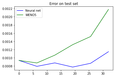
Figure 3.2 plots the time histories of the mean square errors which have been averaged over all test samples. Comparing with WENO5, see Figure 3.2(a), the proposed ML-based method achieves a factor of approximately 8.6 less error in magnitude. Moreover, it is observed that the error by WENO5 increases over time, while the error by our method stays the same in magnitude with slight fluctuation. We further investigate the performance of the proposed method with different CFL numbers, i.e., different time step sizes, and report the result in Figure 3.2(b). We observe that the errors by our method with different CFLs are almost of the same magnitude over time. Figure 3.3 presents the time evolution of deviation in total mass for three test solution trajectories generated by our method. Evidently, the total mass is conserved up to the machine precision as expected.

Although our solver is trained with a data set where each trajectory contains a single square wave, it is observed that the model can be generalized to simulate the advection equation (3.1) with an initial condition consisting of two square waves, as shown in Figure 3.4. Again, our solver demonstrates superior performance over WENO5. It is worth mentioning that the traditional reduced order models employing a direct parameterization of the underlying solution manifold are not capable of such generalization.

Last, we remark that the CFL number cannot be chosen above 2, otherwise the loss would not decrease during training. Such an observation is partly attributed to the fact that the region of dependence for updating one cell average is not completely contained within the 5-cell stencil if the CFL number is greater than 2.

Similar to the previous example, we generate 30 high-resolution solution trajectories, each consisting of one triangle and one square waves with heights randomly sampled from $[0.2,0.8]$ and widths from $[0.2,0.3]$ over the 256-cell grid. By reducing the resolution from 256 to 32 (by a factor of 8), we obtain our training data. For this example, we set the stencil size to be $3$, and the maximum CFL number allowed for training is reduced to $0.975$ based on our numerical experiments. Each solution trajectory in the training data set contains 256 time steps with the CFL number ranging in [0.3,0.975]. The test data are randomly sampled from the same ranges of width and height. To evaluate the performance of the proposed method, we calculate the ground-truth reference solution using WENO5 on a high-resolution grid with 256 cells and then reduce the resolution by a factor of 8 to a coarse grid of 32 cells.

In Figure 3.5, we plot three test samples at several instances of time during forward integration with CFL = 0.6. The proposed ML-based solver generates numerical results with significantly higher resolution of non-smooth structures compared to WENO5. We then present the time histories of the mean square error in Figure 3.6 (a), averaged over all test examples. Our ML-based solver achieves a reduction of error magnitude by a factor of approximately 7.8 compared to the traditional WENO5 solver. Additionally, the error of our solver grows at a much slower rate with time compared to that of WENO5. To further validate our solver, we consider three CFL numbers for testing, and present the time histories of errors in Figure 3.6(b). It is observed that employing a larger CFL results in a smaller error and slower growth in time. Similar to the previous example, our method is mass conservative up to machine precision as demonstrated in Figure 3.7.

We generate 90 solution trajectories, and each initial condition is a square function with heights randomly sampled from $[0.1,1]$ and widths from $[2.5,3.5]$ over the high-resolution grid of 256 cells. By reducing the grid resolution with a factor of 8, we obtain the training data over a 32-cell grid. In addition, each trajectory in the training data contains 30 sequential time steps, with the CFL number ranging in $[0.3,1.2]$. In addition, the center of each square function is randomly sampled from the whole domain $[0,2\pi]$. We set the stencil size to be $5$. Again, the reference solution is generated by WENO5 over the 256-cell grid and down-sampled to the coarse grid of 32 cells. Note that the solution structure is more complicated than previous examples.

We first plot three test samples at several instances of time during forward integration with CFL=0.6 in Figure 3.8. It can be observed that our solver can accurately resolve the solution structures with sharp shock transition and outperforms WENO5.

Figure 3.9(a) shows the time histories of the mean square errors, averaged over all test examples. The proposed method achieves the reduction of the error by a factor of 3.7 in comparison to the WENO5 method. We further report the time histories of errors for the method with three different CFL numbers in Figure 3.9(b), and it is observed the errors are comparable. As demonstrated in Figure 3.10, the proposed method can conserve the total mass up to machine precision.

In this subsection, we present the numerical results for simulating several 2D benchmark advection problem.

The training data is generated by coarsening 30 high-resolution solution trajectories over a $256\times 256$-cell grid by a factor of 8 in each dimension, and each trajectory is initialized as a square wave with height randomly sampled from $[0.5,1]$ and width from $[0.3,0.5]$. One trajectory contains 256 sequential time steps, and the CFL number is chosen within the range of $[0.3,1.8]$. We set the stencil size to be $5\times 5$. For testing, the initial conditions are sampled from the same range of width and height. The reference solution is generated by WENO5 with the mesh of $256\times 256$ cells and down sampled to the original coarse grid.

Figure 3.11 shows 1D cuts of solutions at $y=0.5$ for three test examples at several instances of time during the forward integration with CFL=0.6. It is observed that the proposed method significantly outperforms WENO5 in resolving shocks sharply without introducing spurious oscillations. Furthermore, even after conducting simulations over a long period of 2560 time steps, the proposed method still produces highly accurate results. For a more effective comparison, we also provide the 2D plots of the solutions at time step 256 in Figure 3.12. It can be seen that the solution produced by WENO5 exhibits noticeable smeared shocks, whereas the solution by the proposed method exhibits much sharper shock resolution.

We set the period $T=2$ and the initial condition to be a cosine bell centered at $[c_{x},c_{y}]$:

	$\displaystyle u(x,y)$	$\displaystyle=\frac{1}{2}[1+\cos(\pi r)]$		(3.5)
	$\displaystyle r(x,y)$	$\displaystyle=\min\left[1,6\sqrt{(x-c_{x})^{2}+(y-c_{y})^{2}}\right].$

We initialize 30 trajectories with $c_{x}$ and $c_{y}$ randomly sampled from $[0.25,0.75]$ using a high-resolution mesh of $256\times 256$ cells, which are coarsened by a factor of 8 in each dimension as the training data. Each solution trajectory in the training data contains a sequence of time steps from $t=0$ to $t=T$. We set the stencil size to be $5\times 5$. During testing, the initial conditions are sampled from the same distribution as the training data.

In Figure 3.13, we show the contour plots of the numerical solutions computed by the proposed method and WENO5 along with the reference solution for one test sample. Note that the solution is significantly distorted at $t=T/2$ and returns to its initial state at $t=T$. It is observed that our method produces a result that is in good agreement with the reference solution. However, the solution obtained using WENO5 noticeably deviates from the reference solution due to a large amount of numerical diffusion.

Furthermore, the model which was trained using data from solution trajectories featuring a single bell can generalize to simulate problems with an initial condition containing two bells, as shown in Figure 3.14. The observation is similar to the single bell case. Last, we compare the errors of the numerical solutions by our method and by WENO5 at $t=T$ in Table 1. It is observed that the error of the ML-based SL FV method over the mesh of $32\times 32$ cells is much smaller that of WENO5 with the same mesh size and is comparable to that of WENO5 over the finer mesh of $128\times 128$ cells, demonstrating the efficiency of the proposed method.

References

- [1] Y. Bar-Sinai, S. Hoyer, J. Hickey, and M. P. Brenner. Learning data-driven discretizations for partial differential equations. Proceedings of the National Academy of Sciences, 116(31):15344–15349, 2019.
- [2] Y. Bar-Sinai, S. Hoyer, J. Hickey, and M. P. Brenner. Learning data-driven discretizations for partial differential equations. Proceedings of the National Academy of Sciences, 116(31):15344–15349, 2019.
- [3] A. G. Baydin, B. A. Pearlmutter, A. A. Radul, and J. M. Siskind. Automatic differentiation in machine learning: a survey. Journal of Machine Learning Research, 18:1–43, 2018.
- [4] K. Bhattacharya, B. Hosseini, N. B. Kovachki, and A. M. Stuart. Model reduction and neural networks for parametric PDEs. The SMAI Journal of computational mathematics, 7:121–157, 2021.
- [5] J. Brandstetter, D. Worrall, and M. Welling. Message passing neural pde solvers. arXiv preprint arXiv:2202.03376, 2022.
- [6] Y. Chen, J. Yan, and X. Zhong. Cell-average based neural network method for third order and fifth order KdV type equations. Frontiers in Applied Mathematics and Statistics, 8, 2022.
- [7] Z. Chen, V. Churchill, K. Wu, and D. Xiu. Deep neural network modeling of unknown partial differential equations in nodal space. Journal of Computational Physics, 449:110782, 2022.
- [8] C.-Z. Cheng and G. Knorr. The integration of the vlasov equation in configuration space. Journal of Computational Physics, 22(3):330–351, 1976.
- [9] V. Churchill and D. Xiu. Deep learning of chaotic systems from partially-observed data, 2022. arXiv:2205.08384 [nlin].
- [10] B. Cockburn and C.-W. Shu. Runge–kutta discontinuous galerkin methods for convection-dominated problems. Journal of scientific computing, 16:173–261, 2001.
- [11] R. Courant, E. Isaacson, and M. Rees. On the solution of nonlinear hyperbolic differential equations by finite differences. Communications on pure and applied mathematics, 5(3):243–255, 1952.
- [12] S. Cuomo, V. S. di Cola, F. Giampaolo, G. Rozza, M. Raissi, and F. Piccialli. Scientific machine learning through physics-informed neural networks: Where we are and what’s next, 2022. arXiv:2201.05624 [physics].
- [13] C. Erath, P. H. Lauritzen, and H. M. Tufo. On mass conservation in high-order high-resolution rigorous remapping schemes on the sphere. Monthly weather review, 141(6):2128–2133, 2013.
- [14] S. Gottlieb, C.-W. Shu, and E. Tadmor. Strong stability-preserving high-order time discretization methods. SIAM review, 43(1):89–112, 2001.
- [15] D. Greenfeld, M. Galun, R. Basri, I. Yavneh, and R. Kimmel. Learning to optimize multigrid pde solvers. In International Conference on Machine Learning, pages 2415–2423. PMLR, 2019.
- [16] W. Guo, R. D. Nair, and J.-M. Qiu. A conservative semi-lagrangian discontinuous galerkin scheme on the cubed sphere. Monthly Weather Review, 142(1):457–475, 2014.
- [17] J.-T. Hsieh, S. Zhao, S. Eismann, L. Mirabella, and S. Ermon. Learning neural PDE solvers with convergence guarantees. In International Conference on Learning Representations, 2019.
- [18] A. D. Jagtap, E. Kharazmi, and G. E. Karniadakis. Conservative physics-informed neural networks on discrete domains for conservation laws: Applications to forward and inverse problems. Computer Methods in Applied Mechanics and Engineering, 365:113028, 2020.
- [19] G.-S. Jiang and C.-W. Shu. Efficient implementation of weighted eno schemes. Journal of computational physics, 126(1):202–228, 1996.
- [20] G. Kissas, J. Seidman, L. F. Guilhoto, V. M. Preciado, G. J. Pappas, and P. Perdikaris. Learning operators with coupled attention, 2022. arXiv:2201.01032 [physics].
- [21] D. Kochkov, J. A. Smith, A. Alieva, Q. Wang, M. P. Brenner, and S. Hoyer. Machine learning–accelerated computational fluid dynamics. Proceedings of the National Academy of Sciences, 118(21):e2101784118, 2021.
- [22] L. Á. Larios-Cárdenas and F. Gibou. Error-correcting neural networks for semi-lagrangian advection in the level-set method. Journal of Computational Physics, 471:111623, 2022.
- [23] P. H. Lauritzen, R. D. Nair, and P. A. Ullrich. A conservative semi-lagrangian multi-tracer transport scheme (cslam) on the cubed-sphere grid. Journal of Computational Physics, 229(5):1401–1424, 2010.
- [24] Y. LeCun, Y. Bengio, et al. Convolutional networks for images, speech, and time series. The handbook of brain theory and neural networks, 3361(10):1995, 1995.
- [25] Y. LeCun, B. Boser, J. Denker, D. Henderson, R. Howard, W. Hubbard, and L. Jackel. Handwritten digit recognition with a back-propagation network. Advances in neural information processing systems, 2, 1989.
- [26] Y. LeCun, L. Bottou, Y. Bengio, and P. Haffner. Gradient-based learning applied to document recognition. Proceedings of the IEEE, 86(11):2278–2324, 1998.
- [27] R. J. LeVeque. High-resolution conservative algorithms for advection in incompressible flow. SIAM Journal on Numerical Analysis, 33(2):627–665, 1996.
- [28] Z. Li, N. B. Kovachki, K. Azizzadenesheli, B. Liu, K. Bhattacharya, A. M. Stuart, and A. Anandkumar. Fourier neural operator for parametric partial differential equations. In International Conference on Learning Representations, 2020.
- [29] Z. Li, N. B. Kovachki, K. Azizzadenesheli, B. Liu, K. Bhattacharya, A. M. Stuart, and A. Anandkumar. Neural operator: Graph kernel network for partial differential equations. In ICLR 2020 Workshop on Integration of Deep Neural Models and Differential Equations, 2020.
- [30] I. Loshchilov and F. Hutter. Decoupled weight decay regularization. In International Conference on Learning Representations, 2018.
- [31] L. Lu, P. Jin, G. Pang, Z. Zhang, and G. E. Karniadakis. Learning nonlinear operators via DeepONet based on the universal approximation theorem of operators. Nature Machine Intelligence, 3(3):218–229, Mar. 2021.
- [32] L. Lu, X. Meng, S. Cai, Z. Mao, S. Goswami, Z. Zhang, and G. E. Karniadakis. A comprehensive and fair comparison of two neural operators (with practical extensions) based on fair data. Computer Methods in Applied Mechanics and Engineering, 393:114778, 2022.
- [33] L. Lu, X. Meng, Z. Mao, and G. E. Karniadakis. DeepXDE: A deep learning library for solving differential equations. SIAM Review, 63(1):208–228, 2021.
- [34] L. Lu, R. Pestourie, W. Yao, Z. Wang, F. Verdugo, and S. G. Johnson. Physics-informed neural networks with hard constraints for inverse design. SIAM Journal on Scientific Computing, 43(6):B1105–B1132, 2021.
- [35] L. McClenny and U. Braga-Neto. Self-adaptive physics-informed neural networks using a soft attention mechanism, 2022. arXiv:2009.04544 [cs, stat].
- [36] G. Pang, L. Lu, and G. E. Karniadakis. fPINNs: Fractional physics-informed neural networks. SIAM Journal on Scientific Computing, 41(4), 2019.
- [37] J. Pathak, M. Mustafa, K. Kashinath, E. Motheau, T. Kurth, and M. Day. Using machine learning to augment coarse-grid computational fluid dynamics simulations. arXiv preprint arXiv:2010.00072, 2020.
- [38] C. Qiu and J. Yan. Cell-average based neural network method for hyperbolic and parabolic partial differential equations. arXiv:2107.00813, 2021.
- [39] J.-M. Qiu and A. Christlieb. A conservative high order semi-lagrangian weno method for the vlasov equation. Journal of Computational Physics, 229(4):1130–1149, 2010.
- [40] J.-M. Qiu and C.-W. Shu. Conservative high order semi-lagrangian finite difference weno methods for advection in incompressible flow. Journal of Computational Physics, 230(4):863–889, 2011.
- [41] J.-M. Qiu and C.-W. Shu. Positivity preserving semi-lagrangian discontinuous galerkin formulation: theoretical analysis and application to the vlasov–poisson system. Journal of Computational Physics, 230(23):8386–8409, 2011.
- [42] M. Raissi, P. Perdikaris, and G. Karniadakis. Physics-informed neural networks: A deep learning framework for solving forward and inverse problems involving nonlinear partial differential equations. Journal of Computational Physics, 378:686–707, 2019.
- [43] M. Raissi, P. Perdikaris, and G. E. Karniadakis. Physics informed deep learning (Part I): Data-driven solutions of nonlinear partial differential equations, 2017. arXiv:1711.10561 [cs, math, stat].
- [44] M. Raissi, P. Perdikaris, and G. E. Karniadakis. Physics informed deep learning (Part II): Data-driven discovery of nonlinear partial differential equations, 2017. arXiv:1711.10566 [cs, math, stat].
- [45] D. Ray and J. S. Hesthaven. An artificial neural network as a troubled-cell indicator. Journal of Computational Physics, 367:166–191, 2018.
- [46] A. Robert. A stable numerical integration scheme for the primitive meteorological equations. Atmosphere-Ocean, 19(1):35–46, 1981.
- [47] J. A. Rossmanith and D. C. Seal. A positivity-preserving high-order semi-lagrangian discontinuous galerkin scheme for the vlasov–poisson equations. Journal of Computational Physics, 230(16):6203–6232, 2011.
- [48] E. Sonnendrücker, J. Roche, P. Bertrand, and A. Ghizzo. The semi-lagrangian method for the numerical resolution of the vlasov equation. Journal of computational physics, 149(2):201–220, 1999.
- [49] A. Staniforth and J. Côté. Semi-lagrangian integration schemes for atmospheric models—a review. Monthly weather review, 119(9):2206–2223, 1991.
- [50] Z. Sun, S. Wang, L.-B. Chang, Y. Xing, and D. Xiu. Convolution neural network shock detector for numerical solution of conservation laws. Communications in Computational Physics, 28(5):2075–2108, 2020.
- [51] N. Trask, R. G. Patel, B. J. Gross, and P. J. Atzberger. GMLS-Nets: A framework for learning from unstructured data, 2019. arXiv:1909.05371 [physics, stat].
- [52] Y. Wang, Z. Shen, Z. Long, and B. Dong. Learning to discretize: solving 1D scalar conservation laws via deep reinforcement learning. Communications in Computational Physics, 28(5):2158–2179, 2020.
- [53] J. Yu, L. Lu, X. Meng, and G. E. Karniadakis. Gradient-enhanced physics-informed neural networks for forward and inverse PDE problems. Computer Methods in Applied Mechanics and Engineering, 393:114823, 2022. arXiv:2111.02801 [physics].
- [54] X. Yu and C.-W. Shu. Multi-layer perceptron estimator for the total variation bounded constant in limiters for discontinuous Galerkin methods. La Matematica, 1(1):53–84, 2022.
- [55] J. Zhuang, D. Kochkov, Y. Bar-Sinai, M. P. Brenner, and S. Hoyer. Learned discretizations for passive scalar advection in a two-dimensional turbulent flow. Physical Review Fluids, 6(6):064605, 2021.
- [56] J. Zhuang, D. Kochkov, Y. Bar-Sinai, M. P. Brenner, and S. Hoyer. Learned discretizations for passive scalar advection in a two-dimensional turbulent flow. Physical Review Fluids, 6(6):064605, 2021.