Slowly Rotating Black Holes in Einsteinian Quartic Gravities

We begin with an asymptotic solution in the large-r region. This can be done by taking power series ansatz for $f(r)$ and $g(r)$ :

The coefficients $a_{n}$ and $b_{n}$ determine the behaviour of the solution in the large $r$ region. There is also an homogeneous part to the solution, discussed for $f(r)$ in Khodabakhshi:2020hny, but it decays super-exponentially and can therefore be neglected for our purposes. Inserting these ansatz into the field equations, for $f(r)$ we find

For $g(r)$, the six theories produce different asymptotic expansions, though all have their first correction appear at order $r^{12}$ :

where the $\mathcal{S}_{(4)}^{(3)}$ and $\mathcal{S}_{(4)}^{(4)}$ are equivalent upon making the substitution $\lambda_{(3)}=2\lambda_{(4)}$. Some of the remaining inequivalent theories coincidentally give equivalent asymptotic expansions, as is the case with $\mathcal{S}_{(4)}^{(1)}$ and $\mathcal{S}_{(4)}^{(3)}$.

Before moving on, let us say a few words regarding the homogeneous part of the solution for $g(r)$ in the asymptotic region. To do this we insert $g^{(i)}(r)=g_{1/r}^{(i)}(r)+g_{h}^{(i)}(r)$ into the field equation and keep only the terms that are most significant at large $r$, with $g_{h}^{(i)}(r)$ the homogeneous part of the solution. The resulting equation for $g_{h}^{(i)}(r)$ takes the following form for all six theories:

where there is no summation over the index $(i)$. Here each $\alpha_{(i)}$ is a positive constant whose value depends on the theory in question. The general solution to this equation is

where $I_{\nu}(x)$ and $K_{\nu}(x)$ are the modified Bessel functions of the first and second kinds, respectively, and $\tilde{A}$ and $\tilde{B}$ are constants of integration. Absorbing various constants into the new constants into $A$ and $B$, we may approximate this to first order at large $r$ as the sum of a super-exponentially growing and decaying mode:

Asymptotic flatness demands that we set $A=0$, while the super-exponentially decaying mode clearly falls off far more rapidly than our particular solution in powers of $1/r$, and can therefore be neglected.

As a final note, when we integrate each of the $g_{1/r}^{(6)}(r)$ to obtain the asymptotic form of $p(r)$ in each theory a constant of integration will appear, which we may call $\frac{\Omega_{\infty}}{a}$. This is related to the asymptotic angular velocity of spacetime, as

By suitable choice of Killing coordinates $t$ and $\phi$ we may always set $\Omega_{\infty}=0$ and from now on we will make that choice. This amounts to starting the integration for $p(r)$ at $r=\infty$.

We now wish to solve the equations of motion near the event horizon of the black hole. We begin using an ansatz for $f(r)$ given by

chosen to ensure $f$ has a zero of first order at the horizon $r=r_{+}$, with $T=f^{\prime}(r_{+})/4\pi$ the usual Hawking temperature. Substituting this into the field equation we obtain the following two equations determining $T$ and $M$ from the linear and quadratic-order parts:

These equations can be solved for $M$ and $T$ in terms of $r_{+}$; the resulting expressions are large but are presented in Khodabakhshi:2020hny. Higher-order terms in the field equation do not determine the parameter $a_{2}$ in the above. However, the remaining coefficients $a_{n}$ for $n>2$ can be determined by unwieldy expressions involving $K$, $T$, $M$, and $a_{2}$.

We now use a similar power ansatz for $g(r)$, with the only significant difference being that $g(r)$ is not required to vanish at the event horizon. Using the ansatz

we obtain (rather large) equations giving $g_{n}$ for $n>0$ in terms of $K$, $T$, $M$, $g_{0}$, and near horizon coefficients up to $a_{n+1}$ at most. Like $a_{2}$, $g_{0}$ is an apparently free parameter. The values of both will be numerically determined in the following section, on the basis of producing a smooth fit with the asymptotic approximation already discussed.

Neither the asymptotic nor near horizon solutions are valid for all $r$, and so it is desirable to have a means of interpolating between them. Let us begin by constructing a numerical solution for $f(r)$; the procedure for $g(r)$ will be essentially the same. The idea is to use the initial data from the near horizon expansion in a numerical solver that works both outwards and inwards from the horizon radius. Specifically, for the initial data we write

where $\epsilon$ is a small quantity, chosen to be positive for the outer solution and negative for the inner one. A generic choice of $a_{2}$ will unphysically excite the super-exponentially growing mode. To avoid this and get the asymptotically flat solution, $a_{2}$ must be chosen with high precision. There is generally a unique value of $a_{2}$ at which the numerically generated solution agrees with the asymptotic solution to a high degree of accuracy. To find this $a_{2}$, we must first choose a value $r_{\text{max}}$ with the requirement that the asymptotic solution is a good approximation for $r>r_{\text{max}}$. Then $f(r)$ is recursively solved numerically using different values of $a_{2}$ until one is found for which $f(r)$ agrees with the numerical solution at $r_{\text{max}}$ to the desired precision. Inevitably even this solution will diverge super-exponentially at some point, though that point can be pushed out to larger values of $r$ by increasingly more precise choices of $a_{2}$. A full solution valid for all $r$ is obtained by switching to the asymptotic approximation at $r_{\text{max}}$.

We plot the numerical solution for $f(r)$ in Figure 1 for different values of the coupling $K$. We note that it has two interesting properties: first, that $f(r)$ remains bounded rather than diverging to $-\infty$ as $r\to 0$, and second, that increasing $K$ increases the event horizon radius $r_{+}$.

The idea for constructing the numerical solution for $g(r)$ is the same as for $f(r)$. We construct initial data via

using our near horizon expansion to rewrite $g_{1}$ and $g_{2}$ in terms of $g_{0}$ and the already-determined $a_{2}$. Just as for $a_{2}$, there is a unique choice of $g_{0}$ that avoids exciting the super-exponentially growing mode. We find it in precisely an analogous manner, and construct a full solution for $g(r)$ by switching from the numerical solution evaluated for this choice of $g_{0}$ to the asymptotic solution at a large enough $r$ that the latter becomes a good approximation.

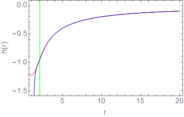
With the solution for $g(r)$ in hand, we may numerically integrate it to obtain $p(r)$ and hence $h(r)=r^{2}p(r)$. We start the integration at $r=\infty$ to $p(r)\rightarrow 0$ as $r\rightarrow\infty$. As discussed, this is equivalent to choosing a frame that does not rotate at infinity. We show these numerical results in Figure 2 for each of the theories. A few interesting observations emerge. First, each of the theories except for that corresponding to $\mathcal{S}_{(4)}^{(5)}$ approaches zero as $r\rightarrow 0$. This behaviour is also observed in ECG and differs from Einstein gravity. $h(r)$ in the $\mathcal{S}_{(4)}^{(5)}$ theory is unique in that it approaches $-\infty$ in the limit $r\rightarrow 0$, but far more sharply and with manifestly different behaviour compared to Einstein gravity.

The near horizon and asymptotic solutions are only valid in their respective regions, and the numerical solution is computationally intensive to generate and inevitably breaks down at sufficiently large distance. Fortunately, we may use another approximation that yields an excellent analytic approximation to the numerical solution everywhere outside the horizon. This is the continued fraction approximation. This approximation has been previously employed in the static case in both ECG Hennigar:2018hza and EQG Khodabakhshi:2020hny and recently in the slowly rotating case in quadratic gravity Sajadi:2023smm. Since the continued fraction equation for $f(r)$ in EQG is the same in the slowly rotating case we study, we can employ it here. We first perform the change of coordinates

so that the spacetime interval outside the horizon is in the range $x\in[0,1)$. We then take an ansatz

where $B(x)$ is given by the continued fraction

Inserting this ansatz in the relevant field equation yields

Furthermore, expanding near the horizon the coefficients $b_{i}$ are straightforwardly obtained. Keeping terms up to $b_{5}$ produces an excellent analytic approximation for $f(r)$, valid for all $r$. In particular, the expressions for the first two coefficients are reasonably simple Khodabakhshi:2020hny:

All higher-order terms in the continued fraction can be written in terms of $a_{2}$, $T$, and $r_{+}$, though the exact expressions are cumbersome, being presented in Appendix C.

To produce an analogous approximation for $g(r)$, a natural first approximation might be to choose an ansatz of the form of (2.31) for $h(r)=r^{2}p(r)$ as it is a similarly dimensionless function. Unfortunately, such an approach leads inevitably to the problem that the continued fraction coefficients are underdetermined – equating terms at order $r^{0}$ involves two continued fraction coefficients, equating terms at order $r^{1}$ involves these and another continued fraction coefficient, and so on. We can, however, construct a continued fraction approximation for $g(r)$ using the following ansatz:

where

We can then numerically integrate this to obtain $p(r)$. While the approximation for $p(r)$ is not analytic, it is nonetheless far less computationally intensive to obtain than constructing a full numerical solution. Note that the exponent $A$ has been left arbitrary. Continued fraction coefficients can be computed with this ansatz for any integer $A>2$, but we found that $A=9$ produced the best agreement with the numerical solution everywhere outside the event horizon. Using this ansatz in an asymptotic expansion, along with the known continued fraction expansion for $f(r)$, yields

To get the continued fraction coefficients $d_{i}$, we once again expand about the event horizon and compare to the near horizon coefficients. We find that generally $d_{n}$ can be expressed in terms of $M$, $r_{h}$, and the near horizon coefficients for $g(r)$ up to $g_{n-1}$, which themselves depend on $g_{0}$, $T$, and the coupling constant. We must therefore use the value of $g_{0}$ numerically determined by the shooting method described above. We find that the first two continued fraction coefficients are given by

The remaining coefficients are given by similar, longer expressions presented in Appendix C. As with $f(r)$, we keep the first five coefficients in the continued fraction. A comparison of the continued fraction approximation to the numerical solution is shown in Figure 3.

The angular velocity of the event horizon is given by

With a metric of the form given by (1.1) this becomes

We construct an expression for the angular velocity in the perturbative regime as follows. Setting $f(r_{+})=0$ in (2.11) we construct an expression for the horizon radius up to second order in $K$. The result is

Using the perturbative expression for $p(r)$, then, we obtain the following for each of the six theories:

where we have defined $\chi=a/M$, and as before $\mathcal{S}_{(4)}^{(3)}$ and $\mathcal{S}_{(4)}^{(4)}$ are equivalent upon making the substitution $\lambda_{(3)}=2\lambda_{(4)}$. These expressions work well in the regime $M\gg\lambda_{(i)}^{1/6}$. For smaller $M$, we must resort to the numerical solutions described in the previous sections.

We now study the geodesics of the slowly rotating solution. The theory to linear order in $a$ is developed in adair2020 for a metric of the form

This analysis results in a linear system of equations for the coordinate functions:

Asymptotically, $j^{2}$ represents the total angular momentum, while $\ell_{z}$ is the component along the $z$-axis (i.e. $\theta=0,\pi$). $\xi$ is the norm of the tangent vector, where

Here we consider geodesics confined to the equatorial plane, which amounts to specializing the previous case by setting $\theta=\pi/2$ and $\dot{\theta}=0$. Note that these constraints combine to enforce $j^{2}=\ell_{z}^{2}$ so that there will be no need in this section to distinguish between these angular momenta. The $r$ equation can be interpreted as being analogous to that of a particle moving in a potential,

References

• (1) D. Lovelock, “Divergence-free tensorial concomitants,” aequationes mathematicae, vol. 4, no. 1, pp. 127–138, 1970.
• (2) D. Lovelock, “The Einstein tensor and its generalizations,” J. Math. Phys., vol. 12, pp. 498–501, 1971.
• (3) J. Oliva and S. Ray, “Classification of Six Derivative Lagrangians of Gravity and Static Spherically Symmetric Solutions,” Phys. Rev., vol. D82, p. 124030, 2010.
• (4) R. C. Myers and B. Robinson, “Black Holes in Quasi-topological Gravity,” JHEP, vol. 1008, p. 067, 2010.
• (5) P. Bueno and P. A. Cano, “Einsteinian cubic gravity,” Phys. Rev. D, vol. 94, no. 10, p. 104005, 2016.
• (6) R. A. Hennigar, D. Kubiznak, and R. B. Mann, “Generalized quasitopological gravity,” Phys. Rev., vol. D95, no. 10, p. 104042, 2017.
• (7) R. A. Hennigar and R. B. Mann, “Black holes in Einsteinian cubic gravity,” Phys. Rev. D, vol. 95, p. 064055, Mar. 2017.
• (8) P. Bueno and P. A. Cano, “Four-dimensional black holes in Einsteinian cubic gravity,” Phys. Rev. D, vol. 94, no. 12, p. 124051, 2016.
• (9) P. Bueno and P. A. Cano, “On black holes in higher-derivative gravities,” Class. Quant. Grav., vol. 34, no. 17, p. 175008, 2017.
• (10) R. A. Hennigar, M. B. J. Poshteh, and R. B. Mann, “Shadows, Signals, and Stability in Einsteinian Cubic Gravity,” Phys. Rev. D, vol. 97, no. 6, p. 064041, 2018.
• (11) M. B. J. Poshteh and R. B. Mann, “Gravitational Lensing by Black Holes in Einsteinian Cubic Gravity,” Phys. Rev. D, vol. 99, no. 2, p. 024035, 2019.
• (12) H. Khodabakhshi, A. Giaimo, and R. B. Mann, “Einstein Quartic Gravity: Shadows, Signals, and Stability,” Phys. Rev. D, vol. 102, no. 4, p. 044038, 2020.
• (13) H. Khodabakhshi and R. B. Mann, “Gravitational Lensing by Black Holes in Einstein Quartic Gravity,” Phys. Rev. D, vol. 103, no. 2, p. 024017, 2021.
• (14) C. Adair, P. Bueno, P. A. Cano, R. A. Hennigar, and R. B. Mann, “Slowly rotating black holes in einsteinian cubic gravity,” Phys. Rev. D, vol. 102, p. 084001, Oct 2020.
• (15) J. Ahmed, R. A. Hennigar, R. B. Mann, and M. Mir, “Quintessential Quartic Quasi-topological Quartet,” JHEP, vol. 05, p. 134, 2017.
• (16) S. N. Sajadi, L. Shahkarami, F. Charmchi, and S. H. Hendi, “Charged black holes in Einsteinian quartic gravity,” Annals Phys., vol. 447, p. 169162, 2022.
• (17) F. Gray, R. A. Hennigar, D. Kubiznak, R. B. Mann, and M. Srivastava, “Generalized Lense-Thirring metrics: higher-curvature corrections and solutions with matter,” JHEP, vol. 04, p. 070, 2022.
• (18) S. N. Sajadi and S. H. Hendi, “Slowly rotating solution of quadratic gravity: An analytical approximation method,” Nucl. Phys. B, vol. 987, p. 116070, 2023.