Exceptional points in cylindrical elastic media with radiation lossPreprint: APS/123-QED

Kei Matsushima Email: matsushima@mech.t.u-tokyo.ac.jp Affiliation: Department of Mechanical Engineering, Graduate School of Engineering, the University of Tokyo
2-11-16 Yayoi, Bunkyo-ku, Tokyo, Japan Yuki Noguchi Affiliation: Department of Mechanical Engineering, Graduate School of Engineering, the University of Tokyo
2-11-16 Yayoi, Bunkyo-ku, Tokyo, Japan Takayuki Yamada Affiliation: Department of Mechanical Engineering, Graduate School of Engineering, the University of Tokyo
2-11-16 Yayoi, Bunkyo-ku, Tokyo, Japan

August 11, 2026

Abstract

Exceptional points (EPs) are singular points on a parameter space at which some eigenvalues (scattering poles) and their corresponding eigenmodes coalesce. This study shows the existence of second- and third-order EPs in cylindrical elastic systems with radiation loss. We consider multilayered cylindrical solids under the plane-strain condition placed in a background elastic or acoustic medium. Elastic and acoustic waves propagating in the background media are subject to the radiation loss. We optimize the radii and the material constants of the multilayered solids, such that some scattering poles coalesce on the complex frequency plane. Some numerical experiments are performed to confirm that the coalescence originates from EPs. We expect that this study provides a new approach for enhancing mechanical sensors.

I Introduction

Exceptional points (EPs) are singularities in a parameter space at which both eigenvalues and eigenmodes coalesce Kato 1995; Berry 2004; Heiss 2012. This simultaneous degeneracy is a unique phenomenon of non-Hermitian systems. Unlike Hermitian systems, non-Hermitian systems have complex eigenvalues, and their imaginary part represents the rate of exponential decay or divergence of resonances in time. Around an EP, two (or more) eigenvalues are associated with each other and draw a Riemann surface of a multivalued root function on the parameter space. This special structure can be observed by continuously changing the parameters around an EP and tracking the corresponding eigenvalues, called EP encircling Dembowski et al. 2001. As the root-like behavior improves the sensitivity of the eigenvalue splitting, a promising application of the non-Hermitian degeneracy is the enhancement of optical and mechanical sensors Wiersig 2014; Wiersig 2016; Chen et al. 2017; Hokmabadi et al. 2019; Xing et al. 2020; Yu et al. 2021; Yuan et al. 2022.

Parity-time (PT) symmetry is one of the most successful approaches for realizing EPs Klaiman et al. 2008; Longhi 2009; Rüter et al. 2010; Özdemir et al. 2019. A system is said to be PT symmetric if the same amount of gain and loss is symmetrically distributed in space. Due to these gain and loss, PT-symmetric systems are non-Hermitian and possibly exhibit EPs. If a system is PT symmetric, the non-Hermitian degeneracy occurs at the PT phase transition points, which can be easily found by tuning the amount of gain and loss Chong et al. 2011.

Although the PT symmetry is an important property when discussing non-Hermitian physics, the EP itself is ubiquitous for various non-Hermitian systems. For example, dielectric microcavities can induce the non-Hermitian degeneracy without gain by tuning the dielectric constant and/or the system geometry Cao and Wiersig 2015. Kullig et al. recently showed the existence of second- and third-order EPs in two-dimensional multilayered microdisk cavities Kullig et al. 2018. They optimized the radii and refractive indices of the layered cavities such that two or three whispering gallary modes coalesce at a single complex frequency. Bulgakov et al. proved that a spheroid exhibits a second-order EP Bulgakov et al. 2021. Abdrabou and Lu studied EPs that arise in two-dimensional multiple scattering systems Abdrabou and Lu 2019. Meanwhile, Gwak et al. realized steady EPs by deforming circular microcavity Gwak et al. 2021. Photonic crystal slabs also exhibit EPs without material gain Zhen et al. 2015; Kamiński et al. 2017; Abdrabou and Lu 2018; Zhou et al. 2018; Abdrabou and Lu 2020.

EPs can also be observed in acoustic and elastic systems. As mentioned, PT symmetry is a convenient platform for discussing non-Hermitian effects on acoustic and elastic wave propagation. Recent studies revealed that the well-known anomalies of PT symmetric systems (e.g., phase transition, asymmetrical reflectance, lasing/anti-lasing, negative refraction, and enhanced sensitivity) are observed in such systems Zhu et al. 2014; Fleury et al. 2015; Fleury et al. 2016; Shi et al. 2016; Christensen et al. 2016; Achilleos et al. 2017; Aurégan and Pagneux 2017; Hou et al. 2018; Wu et al. 2019; Wang et al. 2019; Domínguez-Rocha et al. 2020; Rosa et al. 2021; Farhat et al. 2021; Cai et al. 2022; Yi et al. 2022. However, the existence of EPs in two- and three-dimensional passive elastic systems is still uncertain, except for an open periodic system Mokhtari et al. 2020.

In this study, we numerically show that second- and third-order EPs exist in cylindrical elastic media without gain. The system comprises a multilayered cylindrical solid and background elastic or acoustic medium. The background medium is unbounded in space and induces the energy loss due to the radiation in the radial direction. The solid–solid and solid–fluid coupled problems are solved via Helmholtz decomposition and cylindrical functions. Following Kullig et al. 2018, we optimize the radii and material constants such that two or three eigenvalues (scattering poles) coalesce on the complex frequency plane. Subsequently, the EP encircling is performed around the optimized parameters to confirm that the coalescence originates from the non-Hermitian degeneracy. Moreover, we show that the degenerate poles behave as multivalued root functions around EPs, which is an important property for enhancing mechanical sensors.

II Model

We consider the time-harmonic oscillation of a multilayered solid embedded in a background elastic or acoustic medium as shown in fig. 1. Each solid layer, indexed by the integer $l=1,\ldots,N$ (from innermost to outermost), is a linear, homogeneous, and isotropic elastic medium with mass density $\rho^{(l)}$ and Lamé constants $(\lambda^{(l)},\mu^{(l)})$ . We also assume that the solid is under the plane-strain condition. The in-plane displacement $u$ and stress $\sigma$ are subject to the following two-dimensional Navier–Cauchy equations:

\displaystyle\nabla\cdot\sigma+\rho^{(l)}\omega^{2}u=0,

(1)

where $\omega$ is the angular frequency. The stress tensor $\sigma$ is associated with the displacement $u$ via the following linear relations:

	$\displaystyle\sigma_{ij}$	$\displaystyle=\lambda^{(l)}(\nabla\cdot u)\delta_{ij}+2\mu^{(l)}\varepsilon_{ij},$		(2)
	$\displaystyle\varepsilon_{ij}$	$\displaystyle=\frac{1}{2}\left(\frac{\partial u_{i}}{\partial x_{j}}+\frac{\partial u_{j}}{\partial x_{i}}\right),$		(3)

where $\delta_{ij}$ is the Kronecker delta.

Refer to caption — Figure 1: Multilayered elastic solid embedded in an elastic or acoustic medium. The figure illustrates the case of $N=3$ .

The displacement $u$ and the normal component $\sigma\cdot n$ of the stress are continuous on the solid–solid interfaces, where $n$ is the unit normal vector.

In what follows, we assume that the solid is a cylinder, i.e., the cross section $\Omega^{(l)}$ of Layer $l$ is given by $\Omega^{(l)}=\{x\in\mathbb{R}^{2}\mid R^{(l-1)}<|x|<R^{(l)}\}$ with outer radius $R^{(l)}$ ( $R^{(0)}=0$ ).

A solution of the Navier–Cauchy equations eq. 1 can be sought via Lamé potentials $\phi^{(l)}$ and $\psi^{(l)}$ defined as

\displaystyle u_{i}=\frac{\partial\phi^{(l)}}{\partial x_{i}}+e_{3ij}\frac{\partial\psi^{(l)}}{\partial x_{j}}\quad\text{in }\Omega^{(l)},

(4)

where $e_{ijk}$ is the Levi–Civita symbol Eringen and Suhubi 1975. The potentials decompose the Navier–Cauchy equations eq. 1 into the following Helmholtz equations:

	$\displaystyle\nabla^{2}\phi^{(l)}+\left({\omega/c_{\mathrm{L}}^{(l)}}\right)^{2}\phi^{(l)}=0\quad\text{in }\Omega^{(l)},$		(5)
	$\displaystyle\nabla^{2}\psi^{(l)}+\left({\omega/c_{\mathrm{T}}^{(l)}}\right)^{2}\psi^{(l)}=0\quad\text{in }\Omega^{(l)},$		(6)

where $c_{\mathrm{L}}^{(l)}=\sqrt{(\lambda^{(l)}+2\mu^{(l)})/\rho^{(l)}}$ and $c_{\mathrm{T}}^{(l)}=\sqrt{\mu^{(l)}/\rho^{(l)}}$ are the phase speed of the longitudinal and transverse waves in $\Omega^{(l)}$ , respectively. We can write a solution $(\phi^{(l)},\psi^{(l)})$ as follows for each azimuthal index $m\in\mathbb{Z}$ :

$\displaystyle\phi^{(l)}$	$\displaystyle=A_{\mathrm{L}}^{(l)}J_{m}(\omega r/c_{\mathrm{L}}^{(l)})\exp(\mathrm{i}m\theta)$
	$\displaystyle+B_{\mathrm{L}}^{(l)}H^{(1)}_{m}(\omega r/c_{\mathrm{L}}^{(l)})\exp(\mathrm{i}m\theta),$	(7)
$\displaystyle\psi^{(l)}$	$\displaystyle=A_{\mathrm{T}}^{(l)}J_{m}(\omega r/c_{\mathrm{T}}^{(l)})\exp(\mathrm{i}m\theta)$
	$\displaystyle+B_{\mathrm{T}}^{(l)}H^{(1)}_{m}(\omega r/c_{\mathrm{T}}^{(l)})\exp(\mathrm{i}m\theta),$	(8)

where $(r,\theta)$ is the polar coordinate system. For $l=1,\ldots,N-1$ , the continuity at the interface $r=R^{(l)}$ associates the unknown coefficients $A^{(l)}_{\mathrm{L}}$ , $A^{(l)}_{\mathrm{T}}$ , $B^{(l)}_{\mathrm{L}}$ , and $B^{(l)}_{\mathrm{T}}$ as

\displaystyle M^{(l+1)}(R^{(l)})\begin{pmatrix}A_{\mathrm{L}}^{(l+1)}\\ A_{\mathrm{T}}^{(l+1)}\\ B_{\mathrm{L}}^{(l+1)}\\ B_{\mathrm{T}}^{(l+1)}\end{pmatrix}=M^{(l)}(R^{(l)})\begin{pmatrix}A_{\mathrm{L}}^{(l)}\\ A_{\mathrm{T}}^{(l)}\\ B_{\mathrm{L}}^{(l)}\\ B_{\mathrm{T}}^{(l)}\end{pmatrix},

(9)

where the matrix $M^{(l)}(R)\in\mathbb{C}^{4\times 4}$ is dependent on the frequency $\omega$ , azimuthal index $m$ , and material constants $\rho^{(l)},\lambda^{(l)},\mu^{(l)}$ . The explicit form of $M^{(l)}(R)$ is presented in Appendix A. Any solution should be bounded at $r=0$ ; thus, we have $B_{\mathrm{L}}^{(1)}=B_{\mathrm{T}}^{(1)}=0$ . Accordingly, we can define a 4-by-2 matrix $X$ that gives

\displaystyle X\begin{pmatrix}A_{\mathrm{L}}^{(1)}\\ A_{\mathrm{T}}^{(1)}\end{pmatrix}=\begin{pmatrix}A_{\mathrm{L}}^{(N)}\\ A_{\mathrm{T}}^{(N)}\\ B_{\mathrm{L}}^{(N)}\\ B_{\mathrm{T}}^{(N)}\end{pmatrix}.

(10)

II.1 Solid background

First, we formulate a radiation behavior in the background $r>R^{(N)}$ . When the background medium is an elastic medium with a mass density $\rho$ and Lamé constants $(\lambda,\mu)$ , we define two potentials $\phi$ and $\psi$ as follows in an analogous manner:

\displaystyle u_{i}=\frac{\partial\phi}{\partial x_{i}}+e_{3ij}\frac{\partial\psi}{\partial x_{j}}\quad r>R^{(N)}.

(11)

We are interested in a radiating field without incident waves; therefore, the potentials $\phi$ and $\psi$ are written as

	$\displaystyle\phi$	$\displaystyle=B_{\mathrm{L}}H^{(1)}_{m}(\omega r/c_{\mathrm{L}})\exp(\mathrm{i}m\theta),$		(12)
	$\displaystyle\psi$	$\displaystyle=B_{\mathrm{T}}H^{(1)}_{m}(\omega r/c_{\mathrm{T}})\exp(\mathrm{i}m\theta),$		(13)

where $B_{\mathrm{L}}$ and $B_{\mathrm{T}}$ are constants, and $c_{\mathrm{L}}$ and $c_{\mathrm{T}}$ are defined by $c_{\mathrm{L}}=\sqrt{(\lambda+2\mu)/\rho}$ and $c_{\mathrm{T}}=\sqrt{\mu/\rho}$ , respectively. Similar to Eq. eq. 9, the continuity conditions at $r=R^{(N)}$ equate the coefficients as

\displaystyle Y_{\mathrm{s}}\begin{pmatrix}B_{\mathrm{L}}\\ B_{\mathrm{T}}\end{pmatrix}=Z_{\mathrm{s}}\begin{pmatrix}A_{\mathrm{L}}^{(N)}\\ A_{\mathrm{T}}^{(N)}\\ B_{\mathrm{L}}^{(N)}\\ B_{\mathrm{T}}^{(N)}\end{pmatrix},

(14)

where the 4-by-2 matrix $Y_{\mathrm{s}}$ is defined in Appendix A, and $Z_{\mathrm{s}}=M^{(N)}(R^{(N)})$ . Equations eqs. 10 and 14 give the following linear equations:

\displaystyle\begin{bmatrix}Z_{\mathrm{s}}X&-Y_{\mathrm{s}}\end{bmatrix}\begin{pmatrix}A^{(1)}_{\mathrm{L}}\\ A^{(1)}_{\mathrm{T}}\\ B_{\mathrm{L}}\\ B_{\mathrm{T}}\end{pmatrix}=\begin{pmatrix}0\\ 0\\ 0\\ 0\end{pmatrix}.

(15)

II.2 Fluid background

The fluid background can be modeled in a similar fashion. Let $p$ be a pressure field that satisfies

\displaystyle\nabla^{2}p+(\omega/c)^{2}p=0,\quad r>R^{(N)},

(16)

where the sound speed $c$ is given by the mass density $\rho$ and bulk modulus $\kappa$ of the background fluid as $c=\sqrt{\kappa/\rho}$ . In analogy with the elastic case, the pressure $p$ admits the following solution with a constant $B$ :

\displaystyle p=BH^{(1)}_{m}(\omega r/c)\exp(\mathrm{i}m\theta),\quad r>R^{(N)}.

(17)

Elastic–acoustic coupling is established via the continuity of the displacement and traction at $r=R^{(N)}$ :

	$\displaystyle\sigma\cdot n=-pn,$		(18)
	$\displaystyle u\cdot n=\frac{1}{\rho\omega^{2}}\nabla p\cdot n.$		(19)

Using the polar coordinate system, these conditions are translated into

\displaystyle Y_{\mathrm{f}}B=Z_{\mathrm{f}}\begin{pmatrix}A_{\mathrm{L}}^{(N)}\\ A_{\mathrm{T}}^{(N)}\\ B_{\mathrm{L}}^{(N)}\\ B_{\mathrm{T}}^{(N)}\end{pmatrix},

(20)

where the 3-by-1 matrix $Y_{\mathrm{f}}$ and 3-by-4 matrix $Z_{\mathrm{f}}$ are given in Appendix A.

Finally, we use Eqs. eqs. 10 and 20 to obtain

\displaystyle\begin{bmatrix}Z_{\mathrm{f}}X&-Y_{\mathrm{f}}\end{bmatrix}\begin{pmatrix}A^{(1)}_{\mathrm{L}}\\ A^{(1)}_{\mathrm{T}}\\ B\end{pmatrix}=\begin{pmatrix}0\\ 0\\ 0\end{pmatrix}.

(21)

III Exceptional points

Without any excitation, the time-harmonic oscillation of the multilayered solid is characterized by either Eq. eq. 15 or eq. 21. These linear systems always have a trivial solution (i.e., uniformly $u=0$ ) and possibly nontrivial solutions for discrete angular frequencies $\omega\in\mathbb{C}$ when the determinant of the coefficient matrices becomes zero. These (angular) frequencies are often called quasinormal mode frequencies, complex eigenvalues, or scattering poles. The imaginary part of a scattering pole represents the reciprocal of the lifetime of the corresponding resonance, i.e., exponential decay rate in time induced by the radiation.

The scattering poles are dependent on the system parameters, e.g., the radii and material constants of the layered structure. When two (or more) scattering poles and corresponding resonant modes simultaneously coalesce on the complex $\omega$ -plane for certain system parameters, the parameters are called an exceptional point on the parameter space.

In this study, we show that the multilayered elastic systems exhibit EPs using an optimization algorithm.

To prove that the systems exhibit an EP, we first numerically seek a nontrivial solution of the linear systems eq. 15 and eq. 21. The coefficient matrices depend on $\omega$ nonlinearly; hence, this is a nonlinear eigenvalue problem in terms of $\omega$ . We solve this nonlinear eigenvalue problem using the Sakurai–Sugiura method Asakura et al. 2009. Accordingly, we formally write the nonlinear eigenvalue problem as $\mathcal{A}(\omega)\xi=0$ , where $\mathcal{A}$ is a matrix-valued function. The Sakurai–Sugiura method converts the nonlinear eigenvalue problem into a linear one using contour integrals $\int_{\gamma}W^{H}\mathcal{A}^{-1}(\omega)V\mathrm{d}\omega$ for some full-rank matrices $W$ and $V$ . The linear problem is then solved by a standard eigenvalue solver, which yields the complex eigenvalues (matrix poles) of $\mathcal{A}$ inside the contour path $\gamma$ and corresponding right eigenvector $\xi$ . For more details, see Asakura et al. 2009.

Given $M$ scattering poles $\omega_{i}$ ( $i=1,\ldots,M$ ), we solve the following optimization problem:

\displaystyle\min_{\zeta\in\mathcal{P}}J(\zeta)=\sum_{i\neq j}|\omega_{i}(\zeta)-\omega_{j}(\zeta)|^{2},

(22)

where $\mathcal{P}$ denotes a parameter space. A solution $\zeta$ is an EP of order $M$ in $\mathcal{P}$ if the optimization attains $J=0$ (i.e., $\omega_{1}=\ldots=\omega_{M}$ ), and all the corresponding resonant modes are identical.

IV Results

IV.1 Solid background

In this subsection, we will show that the solid–solid system exhibits second- and third-order EPs. First, we consider the double-layered solid ( $N=2$ ) embedded in a background medium with $(\rho,\lambda,\mu)$ . In analogy with optical layered systems Kullig et al. 2018, we expect that non-Hermitian degeneracy is achieved when two whispering gallary modes coalesce at the same frequency. This can be accomplished when the refractive index of $\Omega^{(1)}$ is larger than that of $\Omega^{(2)}$ . In what follows, we limit the consideration to the case of $m=\pm 8$ . Poisson’s ratio $\nu^{(l)}$ is uniformly $0.3$ for all elastic media.

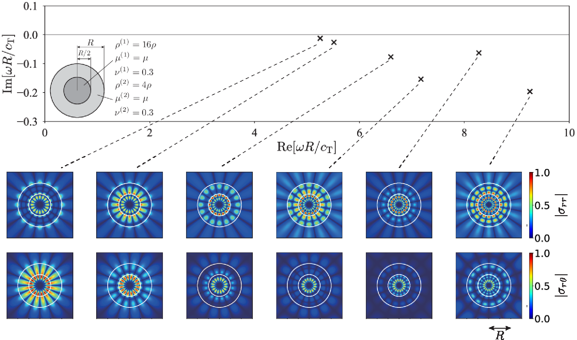
fig. 2 shows the distribution of the scattering poles and corresponding resonant modes for $\rho^{(1)}=16\rho$ , $\rho^{(2)}=4\rho$ , $\mu^{(1)}=\mu^{(2)}=\mu$ , and $R^{(2)}=2R^{(1)}=:R$ . The result clearly indicates that the multilayered elastic system exhibits whispering gallary modes around the solid interfaces. We focus herein on the two neighboring scattering poles, $\omega_{1}R/c_{\mathrm{T}}=5.2513-0.012416\mathrm{i}$ and $\omega_{2}R/c_{\mathrm{T}}=5.5130-0.026387\mathrm{i}$ , and seek a second-order EP on the $R^{(1)}$ – $\rho^{(1)}$ parameter plane.

We performed a two-variable optimization using the Nelder–Mead method Gao and Han 2012 and found an optimal solution $R^{(1)}/R=0.34811$ and $\rho^{(1)}/\rho=35.054$ . This optimized system has two scattering poles at $\omega R/c_{\mathrm{T}}=5.37067922-0.01744497\mathrm{i},5.37067926-0.01744494\mathrm{i}$ . The corresponding resonant modes, shown in fig. 3 (b), also coalesce at the parameters. The simultaneous degeneracy of the poles and resonant modes is a proof of the existence of a second-order EP.

The unique characteristics of second-order EPs can be confirmed by encircling them on a two-variable parameter space. fig. 3 (a) defines a closed elliptic path on the $R^{(1)}$ – $\rho^{(1)}$ plane. The center of the path is the obtained EP. By tracing the path counterclockwise, we compute the two scattering poles on the complex $\omega$ -plane and plot their trajectories in fig. 3 (c). The results show that a single pole does not form a closed path on the $\omega$ -plane although the parameter curve does on the $R^{(1)}$ – $\rho^{(1)}$ plane. Instead, the pair of the two poles closes the trajectory. Equivalently, a single pole forms a closed loop when the parameter curve encircles the EP twice. This feature is analogous to the multivalued square root function on the complex plane.

We discuss this square root-like behavior by computing the pole pair for various parameters $R^{(1)}$ and $\rho^{(1)}$ around the EP. fig. 4 illustrates the result. The pair forms two crossed sheets that branch off at the EP. This structure is similar to the Riemann surfaces of the square root function. These results imply that the obtained EP originates from a branch point of a complex-valued function, although it is not explicit in the equation eq. 15.

We now show that a triple-layered solid exhibits a third-order EP by starting with the following parameters:

•

Mass density $\rho^{(1)}=64\rho,\,\rho^{(2)}=16\rho,\,\rho^{(3)}=4\rho$
•

Shear modulus $\mu^{(1)}=\mu^{(2)}=\mu^{(3)}=\mu$
•

Radii $R^{(1)}=R/4$ , $R^{(2)}=R/2$ , $R^{(3)}=:R$ .

We chose three scattering poles $\omega R/c_{\mathrm{T}}=5.2088-0.005504\mathrm{i}$ , $5.3657-0.016873\mathrm{i}$ , and $5.5851-0.017023\mathrm{i}$ and optimized the five parameters $R^{(1)}$ , $R^{(2)}$ , $\rho^{(1)}$ , $\rho^{(2)}$ , and $\rho^{(3)}$ to find an EP.

The optimized parameters are $R^{(1)}/R=0.11969$ , $R^{(2)}=0.38351$ , $\rho^{(1)}/\rho=270.69$ , $\rho^{(2)}/\rho=25.971$ , and $\rho^{(3)}/\rho=3.57568$ . The optimized system has three poles $\omega R/c_{\mathrm{T}}$ at $5.6385-0.019254\mathrm{i}$ , $5.6387-0.019293\mathrm{i}$ , and $5.6386-0.019242\mathrm{i}$ , which are almost degenerated. Moreover, fig. 5 (b) show that not only the pole values but also corresponding resonant modes coalesced at the point. We confirm that the degeneracy arose from a third-order EP by performing the EP encircling on the $R^{(2)}$ – $\rho^{(2)}$ parameter space. Namely, we continuously change the values of $R^{(2)}$ and $\rho^{(2)}$ and calculate the poles on the complex $\omega$ -plane while the other parameters remain fixed.

fig. 5 depicts the results. As with the previous discussion on the second-order EP, we move the two parameters counterclockwise along the elliptic path shown in fig. 5 (a). fig. 5 (c) plots the trajectories of the three poles. The three trajectories form a single closed curve, which is a well-known characteristic of third-order EPs. Another important property is the asymptotic behavior of the degenerate poles when the parameters are perturbed at the third-order EP. We fix the parameter $\rho^{(2)}$ at the EP and perturb the other parameter as $R^{(2)}=0.38351R+\Delta_{R}$ , where $\Delta_{R}$ is sufficiently small. The three poles should deviate from the degenerate value as the value of $\Delta_{R}$ increases. We define the variation as $\Delta_{\omega}=\mathrm{max}_{i\neq j}|\omega_{i}-\omega_{j}|$ , which is a function of $\Delta_{R}$ , and plot its values in fig. 6. The result shows that the variation asymptotically behaves as $O(\Delta_{R}^{1/3})$ , while the second-order EP exhibits the square-root behavior. This is another characteristic of third-order EPs.

IV.2 Fluid background

When the layered solid is immersed in a fluid medium, the system loses its energy due to the acoustic wave radiation. Here, we use the same optimization approach to show that the solid–fluid coupled systems exhibit EPs.

In this subsection, we fix the mass density $\rho>0$ , bulk modulus $\kappa>0$ , and outer radius $R^{(N)}=:R$ . We first assume $N=2$ and compute the scattering poles for $\rho^{(1)}=16\rho$ , $\rho^{(2)}=4\rho$ , $\mu^{(1)}=\mu^{(2)}=\kappa$ , and $R^{(1)}=R/2$ . Subsequenctly, we chose two scattering poles $\omega R/c$ at $6.4436-0.029230\mathrm{i}$ and $7.0062-0.035093\mathrm{i}$ and optimize the parameters $\rho^{(1)}$ and $R^{(1)}$ .

fig. 7 shows the results of the optimization and EP encircling. The parameter optimization successfully minimizes the objective function $J$ with two poles $\omega R/c$ at $6.5056469-0.0240559\mathrm{i}$ and $6.5056469-0.0240557\mathrm{i}$ . The degenerate resonant modes are plotted in fig. 7 (b). Encircling the obtained parameters $R^{(1)}/R=0.29400$ and $\rho^{(1)}/\rho=54.145$ on the $R^{(1)}$ – $\rho^{(1)}$ plane as shown in fig. 7 (a), we obtain the trajectories of the two poles on the complex $\omega$ -plane (fig. 7 (c)) with the same structures as the second-order EP of the solid–solid model. From the results, we conclude that a second-order EP exists within the parameter path.

Finally, we shall prove the existence of a third-order EP. As with the solid–solid model, we use the triple-layered solid ( $N=3$ ) with the following parameters:

•

Mass density $\rho^{(1)}=64\rho,\,\rho^{(2)}=16\rho,\,\rho^{(3)}=4\rho$
•

Shear modulus $\mu^{(1)}=\mu^{(2)}=\mu^{(3)}=\kappa$
•

Radii $R^{(1)}=R/4$ , $R^{(2)}=R/2$ , $R^{(3)}=:R$ .

The system has three scattering poles $\omega R/c$ at $6.4222-0.022268\mathrm{i}$ , $6.7600-0.025502\mathrm{i}$ , and $7.2757-0.019004\mathrm{i}$ . We optimize the parameters $R^{(1)}$ , $R^{(2)}$ , $\rho^{(1)}$ , $\rho^{(2)}$ , and $\rho^{(3)}$ with the other parameters fixed. fig. 8 illustrates the results. The three poles almost coalesce at $R^{(1)}/R=0.12678$ , $R^{(2)}=0.40343$ , $\rho^{(1)}/\rho=200.46$ , $\rho^{(2)}/\rho=19.400$ , and $\rho^{(3)}/\rho=2.7136$ with $\omega_{1}R/c=7.7966-0.094927\mathrm{i}$ , $\omega_{2}R/c=7.7971-0.094901\mathrm{i}$ , and $\omega_{3}R/c=7.7968-0.094903\mathrm{i}$ . Their resonant modes are also degenerated as shown in fig. 8 (b). The existence of a third-order EP is confirmed by the EP encircling. fig. 8 (a) and (c) present the results of the EP encircling. Like the solid–solid case (fig. 5), we observe a three-fold structure on the complex $\omega$ -plane, which implies the existence of a three-order EP.

V Conclusions

This study discussed the non-Hermitian degeneracy of the scattering poles in cylindrical elastic systems with radiation loss. We first formulated two-dimensional elastodynamic problems using Lamé potentials and cylindrical functions. Some system parameters were optimized such that two or three scattering poles coalesce on the complex frequency plane. We performed the EP encircling around the optimized parameters to confirm the existence of second- and third-order EPs. We found that the sensitivity of degenerate poles at a third-order EP is $O(\Delta^{1/3})$ , where $\Delta$ is a system parameter. This anomalous sensitivity allows enhancement on mechanical sensors, such as pressure/stress sensing and defect detection.

Acknowledgements.

This work was supported by JSPS KAKENHI Grant Number JP22K14166.

Appendix A Explicit forms of the matrices

To formulate Eq. eq. 9, we use the continuity of $u$ and $\sigma\cdot n$ , which is equivalent to that of $u_{r}$ , $u_{\theta}$ , $\sigma_{rr}$ , and $\sigma_{r\theta}$ . After some calculations Eringen and Suhubi 1975, we have

\displaystyle M^{(l)}(r)=\begin{bmatrix}U^{(l)}_{1}(r)&U^{(l)}_{2}(r)&\tilde{U}^{(l)}_{1}(r)&\tilde{U}^{(l)}_{2}(r)\\ V^{(l)}_{1}(r)&V^{(l)}_{2}(r)&\tilde{V}^{(l)}_{1}(r)&\tilde{V}^{(l)}_{2}(r)\\ T^{(l)}_{11}(r)&T^{(l)}_{12}(r)&\tilde{T}^{(l)}_{11}(r)&\tilde{T}^{(l)}_{12}(r)\\ T^{(l)}_{41}(r)&T^{(l)}_{42}(r)&\tilde{T}^{(l)}_{41}(r)&\tilde{T}^{(l)}_{42}(r)\end{bmatrix},

(23)

where

$\displaystyle T^{(l)}_{11}$	$\displaystyle=\frac{2\mu^{(l)}}{r^{2}}\biggl[(m^{2}+m-\frac{1}{2}(k_{\mathrm{T}}^{(l)})^{2}r^{2})J_{m}(k_{\mathrm{L}}^{(l)}r)$
	$\displaystyle\hskip 100.0pt-k_{\mathrm{L}}^{(l)}rJ_{m-1}(k_{\mathrm{L}}^{(l)}r)\biggr],$	(24)
$\displaystyle T^{(l)}_{12}$	$\displaystyle=\frac{2\mu^{(l)}}{r^{2}}\bigl[-\mathrm{i}m\bigl((m+1)J_{m}(k_{\mathrm{T}}^{(l)}r)$
	$\displaystyle\hskip 100.0pt-k_{\mathrm{T}}^{(l)}rJ_{m-1}(k_{\mathrm{T}}^{(l)}r)\bigr)\bigr],$	(25)
$\displaystyle T^{(l)}_{41}$	$\displaystyle=\frac{2\mu^{(l)}}{r^{2}}\bigl[-\mathrm{i}m\bigl((m+1)J_{m}(k_{\mathrm{L}}^{(l)}r)$
	$\displaystyle\hskip 100.0pt-k_{\mathrm{L}}^{(l)}rJ_{m-1}(k_{\mathrm{L}}^{(l)}r)\bigr)\bigr],$	(26)
$\displaystyle T^{(l)}_{42}$	$\displaystyle=\frac{2\mu^{(l)}}{r^{2}}\biggl[-(m^{2}+m-\frac{1}{2}(k_{\mathrm{T}}^{(l)})^{2}r^{2})J_{m}(k_{\mathrm{T}}^{(l)}r)$
	$\displaystyle\hskip 100.0pt+k_{\mathrm{T}}^{(l)}rJ_{m-1}(k_{\mathrm{T}}^{(l)}r)\biggr],$	(27)
$\displaystyle U^{(l)}_{1}$	$\displaystyle=k_{\mathrm{L}}^{(l)}J^{\prime}_{m}(k_{\mathrm{L}}^{(l)}r),$	(28)
$\displaystyle U^{(l)}_{2}$	$\displaystyle=\frac{\mathrm{i}m}{r}J_{m}(k_{\mathrm{T}}^{(l)}r),$	(29)
$\displaystyle V^{(l)}_{1}$	$\displaystyle=\frac{\mathrm{i}m}{r}J_{m}(k_{\mathrm{L}}^{(l)}r),$	(30)
$\displaystyle V^{(l)}_{2}$	$\displaystyle=-k_{\mathrm{T}}^{(l)}J^{\prime}_{m}(k_{\mathrm{T}}^{(l)}r).$	(31)

The functions with the tilde are defined by replacing $J_{m}$ with $H^{(1)}_{m}$ .

Similarly, the matrix $Y_{\mathrm{s}}$ is given by

\displaystyle Y_{\mathrm{s}}=\begin{bmatrix}\tilde{U}_{1}(R^{(N)})&\tilde{U}_{2}(R^{(N)})\\ \tilde{V}_{1}(R^{(N)})&\tilde{V}_{2}(R^{(N)})\\ \tilde{T}_{11}(R^{(N)})&\tilde{T}_{12}(R^{(N)})\\ \tilde{T}_{41}(R^{(N)})&\tilde{T}_{42}(R^{(N)})\end{bmatrix}.

(32)

The solid–fluid coupling matrices are written as

	$\displaystyle Z_{\mathrm{f}}$	$\displaystyle=\begin{bmatrix}T^{(l)}_{11}(R^{(N)})&T^{(l)}_{12}(R^{(N)})&\tilde{T}^{(l)}_{11}(R^{(N)})&\tilde{T}^{(l)}_{12}(R^{(N)})\\ T^{(l)}_{41}(R^{(N)})&T^{(l)}_{42}(R^{(N)})&\tilde{T}^{(l)}_{41}(R^{(N)})&\tilde{T}^{(l)}_{42}(R^{(N)})\\ U^{(l)}_{1}(R^{(N)})&U^{(l)}_{2}(R^{(N)})&\tilde{U}^{(l)}_{1}(R^{(N)})&\tilde{U}^{(l)}_{2}(R^{(N)})\end{bmatrix},$		(33)
	$\displaystyle Y_{\mathrm{f}}$	$\displaystyle=\begin{bmatrix}-H^{(1)}_{n}(\omega R^{(N)}/c)\\ 0\\ \frac{1}{c\rho\omega}H^{(1)\prime}_{n}(\omega R^{(N)}/c)\end{bmatrix}.$		(34)

References

Kato (1995) T. Kato, Perturbation Theory for Linear Operators, Classics in Mathematics, Vol. 132 (Springer, Berlin, Heidelberg, 1995).
Berry (2004) M. Berry, Physics of nonhermitian degeneracies, Czechoslovak Journal of Physics 54, 1039 (2004).
Heiss (2012) W. D. Heiss, The physics of exceptional points, Journal of Physics A: Mathematical and Theoretical 45, 444016 (2012).
Dembowski et al. (2001) C. Dembowski, H.-D. Gräf, H. L. Harney, A. Heine, W. D. Heiss, H. Rehfeld, and A. Richter, Experimental observation of the topological structure of exceptional points, Physical Review Letters 86, 787 (2001).
Wiersig (2014) J. Wiersig, Enhancing the sensitivity of frequency and energy splitting detection by using exceptional points: Application to microcavity sensors for single-particle detection, Physical Review Letters 112, 203901 (2014).
Wiersig (2016) J. Wiersig, Sensors operating at exceptional points: General theory, Physical Review A 93, 033809 (2016).
Chen et al. (2017) W. Chen, Ş. Kaya Özdemir, G. Zhao, J. Wiersig, and L. Yang, Exceptional points enhance sensing in an optical microcavity, Nature 548, 192 (2017).
Hokmabadi et al. (2019) M. P. Hokmabadi, A. Schumer, D. N. Christodoulides, and M. Khajavikhan, Non-Hermitian ring laser gyroscopes with enhanced Sagnac sensitivity, Nature 576, 70 (2019).
Xing et al. (2020) T. Xing, Z. Pan, Y. Tao, G. Xing, R. Wang, W. Liu, E. Xing, J. Rong, J. Tang, and J. Liu, Ultrahigh sensitivity stress sensing method near the exceptional point of parity-time symmetric systems, Journal of Physics D: Applied Physics 53, 205102 (2020).
Yu et al. (2021) D. Yu, M. Humar, K. Meserve, R. C. Bailey, S. N. Chormaic, and F. Vollmer, Whispering-gallery-mode sensors for biological and physical sensing, Nature Reviews Methods Primers 1, 1 (2021).
Yuan et al. (2022) J. Yuan, L. Geng, J. Huang, Q. Guo, J. Yang, G. Hu, and X. Zhou, Exceptional points induced by time-varying mass to enhance the sensitivity of defect detection, Physical Review Applied 18, 064055 (2022).
Klaiman et al. (2008) S. Klaiman, U. Günther, and N. Moiseyev, Visualization of branch points in $\mathcal{P}\mathcal{T}$ -symmetric waveguides, Physical Review Letters 101, 080402 (2008).
Longhi (2009) S. Longhi, Bloch oscillations in complex crystals with $\mathcal{P}\mathcal{T}$ symmetry, Physical Review Letters 103, 123601 (2009).
Rüter et al. (2010) C. E. Rüter, K. G. Makris, R. El-Ganainy, D. N. Christodoulides, M. Segev, and D. Kip, Observation of parity–time symmetry in optics, Nature Physics 6, 192 (2010).
Özdemir et al. (2019) Ş. K. Özdemir, S. Rotter, F. Nori, and L. Yang, Parity–time symmetry and exceptional points in photonics, Nature Materials 18, 783 (2019).
Chong et al. (2011) Y. D. Chong, L. Ge, and A. D. Stone, $\mathcal{P}\mathcal{T}$ -Symmetry Breaking and Laser-Absorber Modes in Optical Scattering Systems, Physical Review Letters 106, 093902 (2011).
Cao and Wiersig (2015) H. Cao and J. Wiersig, Dielectric microcavities: Model systems for wave chaos and non-Hermitian physics, Reviews of Modern Physics 87, 61 (2015).
Kullig et al. (2018) J. Kullig, C.-H. Yi, M. Hentschel, and J. Wiersig, Exceptional points of third-order in a layered optical microdisk cavity, New Journal of Physics 20, 083016 (2018).
Bulgakov et al. (2021) E. Bulgakov, K. Pichugin, and A. Sadreev, Exceptional points in a dielectric spheroid, Physical Review A 104, 053507 (2021).
Abdrabou and Lu (2019) A. Abdrabou and Y. Y. Lu, Exceptional points for resonant states on parallel circular dielectric cylinders, Journal of the Optical Society of America B 36, 1659 (2019).
Gwak et al. (2021) S. Gwak, H. Kim, H.-H. Yu, J. Ryu, C.-M. Kim, C.-H. Yi, and C.-H. Yi, Rayleigh scatterer-induced steady exceptional points of stable-island modes in a deformed optical microdisk, Optics Letters 46, 2980 (2021).
Zhen et al. (2015) B. Zhen, C. W. Hsu, Y. Igarashi, L. Lu, I. Kaminer, A. Pick, S.-L. Chua, J. D. Joannopoulos, and M. Soljačić, Spawning rings of exceptional points out of Dirac cones, Nature 525, 354 (2015).
Kamiński et al. (2017) P. M. Kamiński, A. Taghizadeh, O. Breinbjerg, J. Mørk, and S. Arslanagić, Control of exceptional points in photonic crystal slabs, Optics Letters 42, 2866 (2017).
Abdrabou and Lu (2018) A. Abdrabou and Y. Y. Lu, Exceptional points of resonant states on a periodic slab, Physical Review A 97, 063822 (2018).
Zhou et al. (2018) H. Zhou, C. Peng, Y. Yoon, C. W. Hsu, K. A. Nelson, L. Fu, J. D. Joannopoulos, M. Soljačić, and B. Zhen, Observation of bulk Fermi arc and polarization half charge from paired exceptional points, Science 359, 1009 (2018).
Abdrabou and Lu (2020) A. Abdrabou and Y. Y. Lu, Exceptional points of Bloch eigenmodes on a dielectric slab with a periodic array of cylinders, Physica Scripta 95, 095507 (2020).
Zhu et al. (2014) X. Zhu, H. Ramezani, C. Shi, J. Zhu, and X. Zhang, $\mathcal{P}\mathcal{T}$ -symmetric acoustics, Physical Review X 4, 031042 (2014).
Fleury et al. (2015) R. Fleury, D. Sounas, and A. Alù, An invisible acoustic sensor based on parity-time symmetry, Nature Communications 6, 5905 (2015).
Fleury et al. (2016) R. Fleury, D. L. Sounas, and A. Alù, Parity-time symmetry in acoustics: Theory, devices, and potential applications, IEEE Journal of Selected Topics in Quantum Electronics 22, 121 (2016).
Shi et al. (2016) C. Shi, M. Dubois, Y. Chen, L. Cheng, H. Ramezani, Y. Wang, and X. Zhang, Accessing the exceptional points of parity-time symmetric acoustics, Nature Communications 7, 11110 (2016).
Christensen et al. (2016) J. Christensen, M. Willatzen, V. R. Velasco, and M.-H. Lu, Parity-time synthetic phononic media, Physical Review Letters 116, 207601 (2016).
Achilleos et al. (2017) V. Achilleos, G. Theocharis, O. Richoux, and V. Pagneux, Non-Hermitian acoustic metamaterials: Role of exceptional points in sound absorption, Physical Review B 95, 144303 (2017).
Aurégan and Pagneux (2017) Y. Aurégan and V. Pagneux, $\mathcal{P}\mathcal{T}$ -symmetric scattering in flow duct acoustics, Physical Review Letters 118, 174301 (2017).
Hou et al. (2018) Z. Hou, H. Ni, and B. Assouar, $\mathcal{P}\mathcal{T}$ -symmetry for elastic negative refraction, Physical Review Applied 10, 044071 (2018).
Wu et al. (2019) Q. Wu, Y. Chen, and G. Huang, Asymmetric scattering of flexural waves in a parity-time symmetric metamaterial beam, The Journal of the Acoustical Society of America 146, 850 (2019).
Wang et al. (2019) X. Wang, X. Fang, D. Mao, Y. Jing, and Y. Li, Extremely asymmetrical acoustic metasurface mirror at the exceptional point, Physical Review Letters 123, 214302 (2019).
Domínguez-Rocha et al. (2020) V. Domínguez-Rocha, R. Thevamaran, F. M. Ellis, and T. Kottos, Environmentally induced exceptional points in elastodynamics, Physical Review Applied 13, 014060 (2020).
Rosa et al. (2021) M. I. N. Rosa, M. Mazzotti, and M. Ruzzene, Exceptional points and enhanced sensitivity in PT-symmetric continuous elastic media, Journal of the Mechanics and Physics of Solids 149, 104325 (2021).
Farhat et al. (2021) M. Farhat, P.-Y. Chen, S. Guenneau, and Y. Wu, Self-dual singularity through lasing and antilasing in thin elastic plates, Physical Review B 103, 134101 (2021).
Cai et al. (2022) R. Cai, Y. Jin, Y. Li, T. Rabczuk, Y. Pennec, B. Djafari-Rouhani, and X. Zhuang, Exceptional points and skin modes in non-Hermitian metabeams, Physical Review Applied 18, 014067 (2022).
Yi et al. (2022) J. Yi, Z. Ma, R. Xia, M. Negahban, C. Chen, and Z. Li, Structural periodicity dependent scattering behavior in parity-time symmetric elastic metamaterials, Physical Review B 106, 014303 (2022).
Mokhtari et al. (2020) A. A. Mokhtari, Y. Lu, Q. Zhou, A. V. Amirkhizi, and A. Srivastava, Scattering of in-plane elastic waves at metamaterial interfaces, International Journal of Engineering Science 150, 103278 (2020).
Eringen and Suhubi (1975) A. C. Eringen and E. S. Suhubi, Elastodynamics, Vol. II, Linear Theory (Academic Press, 1975).
Asakura et al. (2009) J. Asakura, T. Sakurai, H. Tadano, T. Ikegami, and K. Kimura, A numerical method for nonlinear eigenvalue problems using contour integrals, JSIAM Letters 1, 52 (2009).
Gao and Han (2012) F. Gao and L. Han, Implementing the Nelder-Mead simplex algorithm with adaptive parameters, Computational Optimization and Applications 51, 259 (2012).