Properties of the eigenmodes and quantum-chaotic scattering in a superconducting microwave Dirac billiard with threefold rotational symmetry
Abstract
We report on experimental studies that were performed with a microwave Dirac billiard (DB), that is, a flat resonator containing metallic cylinders arranged on a triangular grid, whose shape has a threefold rotational () symmetry. Its band structure exhibits two Dirac points (DPs) that are separated by a nearly flat band. We present a procedure which we employed to identify eigenfrequencies and to separate the eigenstates according to their transformation properties under rotation by into the three subspaces. This allows us to verify previous numerical results of Ref. [W. Zhang and B. Dietz, Phys. Rev. B 104, 064310 (2021)], thus confirming that the properties of the eigenmodes coincide with those of artificial graphene around the lower DP, and are well described by a tight-binding model (TBM) for a honeycomb-kagome lattice of corresponding shape. Above all, we investigate properties of the wave-function components in terms of the fluctuation properties of the measured scattering matrix, which are numerically not accessible. They are compared to random-matrix theory predictions for quantum-chaotic scattering systems exhibiting extended or localized states in the interaction region, that is, the DB. Even in regions, where the wave functions are localized, the spectral properties coincide with those of typical quantum systems with chaotic classical counterpart.
I Introduction


Superconducting microwave Dirac billiards (DBs) have been used since more than a decade to investigate fluctuation properties in the energy spectra of artificial graphene and fullerene structures Bittner et al. 2010; Bittner et al. 2012; Dietz et al. 2013; Dietz et al. 2015a; Iachello et al. 2015; Dietz and Richter 2015; Dietz et al. 2015b; Dietz et al. 2016; Dietz and Richter 2019. The experiments presented in this work were performed with the DB shown schematically in Fig. 1, whose shape has a symmetry. The frequency was restricted to the range of the lowest transverse-magnetic (TM) mode, where the electric-field strength is perpendicular to the resonator plane and thus is governed by the scalar Helmholtz equation with Dirichlet boundary conditions (BCs) at the sidewalls of the cavity and cylinders. The Helmholtz equation is mathematically identical to the Schrödinger equation of a quantum billiard (QB) of corresponding shape, into which scatterers are inserted at the positions of the cylinders. The crucial advantage of such resonators as compared to honeycomb structures constructed from dielectric disks Kuhl et al. 2010 is that superconducting high-precision measurements can be performed, which is indispensable for the determination of complete sequences of resonance frequencies.
The band structure of propagating modes of the DB exhibits two Dirac points (DPs), where the first and second, respectively, the fourth and fifth band touch each other conically, and a nearly flat third band (FB) in between. It is reminiscent of that of a honeycomb-kagome billiard (HKB) whose sites form a combination of a honeycomb and a kagome sublattice Jacqmin et al. 2014; Lan et al. 2012; Lu et al. 2017a; Zhong et al. 2017; Maimaiti et al. 2020; Zhang and Dietz 2021; see the upmost inset of Fig. 1. Indeed, below the FB the electric-field intensities are maximal at the voids, that are located at the centers of three neighboring metallic cylinders (grey disks), marked with red and turquoise dots in Fig. 1 and form a honeycomb structure. In the frequency range of the FB they are maximal at the centers between adjacent cylinders, marked by black dots, that are at the sites of a kagome lattice, and above the FB on all sites of the HKB Maimaiti et al. 2020; Zhang and Dietz 2021. We demonstrated that below the FB the properties of DBs are well captured by a tight-binding model (TBM) for a graphene billiard (GB) Dietz et al. 2015a; Dietz et al. 2015b; Dietz et al. 2016, and generally by one for a HKB Maimaiti et al. 2020; Zhang and Dietz 2021. Dirac points are a characteristic of graphene, that attracted a lot of attention Novoselov et al. 2004; Beenakker 2008; Castro Neto et al. 2009 because in the region of the conical valleys graphene features relativistic phenomena DiVincenzo and Mele 1984; Novoselov et al. 2004; Geim and Novoselov 2007; Avouris et al. 2007; Miao et al. 2007; Ponomarenko et al. 2008; Beenakker 2008; Zhang and Liu 2008; Castro Neto et al. 2009; Abergel et al. 2010; Zandbergen and de Dood 2010, which triggered numerous realizations Polini et al. 2013 of artificial graphene Parimi et al. 2004; Joannopoulos et al. 2008; Bittner et al. 2010; Kuhl et al. 2010; Singha et al. 2011; Nádvorník et al. 2012; Gomes et al. 2012; Tarruell et al. 2012; Uehlinger et al. 2013; Rechtsman et al. 2013a; Rechtsman et al. 2013b; Khanikaev et al. 2013; Wang et al. 2014; Shi et al. 2015; Bellec et al. 2013a; Bellec et al. 2013b; Bellec et al. 2014. In the vicinity of the band edges (BEs) the spectral properties coincide with those of a nonrelativistic QB of corresponding shape Dietz et al. 2015a; Dietz et al. 2013; Dietz et al. 2016.
The classical dynamics of a billiard with the shape of the DB shown in Fig. 1 is chaotic Dembowski et al. 2000; Zhang and Dietz 2021. According to the Bohigas-Giannoni-Schmit conjecture the fluctuation properties in the energy spectra of nonrelativistic quantum systems with a chaotic classical counterpart are universal Berry and Tabor 1977; Berry 1979; Casati et al. 1980; Bohigas et al. 1984 and coincide with those of random matrices from the Gaussian orthogonal ensemble (GOE) for time-reversal () invariant systems and the Gaussian unitary ensemble (GUE) if invariance is violated. Yet there also exist billiards with certain shapes which do not comply with this conjecture. Examples are billiards whose shape has symmetry Leyvraz et al. 1996; Dembowski et al. 2000; Dembowski et al. 2003, a unidirectional classical dynamics Knill 1998; Gutkin 2007; Veble et al. 2007; Dietz et al. 2014 or nanoelectromechanical systems consisting of a circular quantum dot on a suspended nanoscopic dielectric plate Rego et al. 2005; Gusso et al. 2006. Their spectral properties may coincide with those of generic chaotic systems with violated time-reversal invariance even though it is preserved. The boundary of the DB has a symmetry. We, actually, chose the same shape as in the experiments which were performed 20 years ago with a superconducting microwave billiard in the range below the cutoff frequency of the first transverse-electric mode, to investigate the spectral properties of the corresponding quantum billiard Dembowski et al. 2000; Dembowski et al. 2003. Interest in this QB arose due to theoretical predictions Robbins 1989a; Leyvraz et al. 1996; Keating and Robbins 1997; Joyner et al. 2012 that the spectral properties of part of the spectrum coincide with those of random matrices from the GUE. The origin of these discrepancies are outlined in Sec. II.
The objective of Zhang and Dietz 2021 and the present work was the numerical and experimental study of the properties of DBs and corresponding GBs and HKBs, whose boundary has a symmetry, especially in the relativistic region aorund the DPs. In the region of the conical valleys, that are located on, respectively, three of the corners of the first Brillouin zone Wallace 1947, the two sets of valley eigenstates are well described by Dirac Hamiltonians for massless spin-1/2 quasiparticles Beenakker 2008; Castro Neto et al. 2009. Therefore, we also investigated in Ref. Zhang and Dietz 2021 properties of relativistic neutrino billiards (NBs) of corresponding shape. They were introduced in Ref. Berry and Mondragon 1987, and are governed by the Weyl equation Weyl 1929 for a spin-1/2 particle. The associated Dirac Hamiltonian is not invariant under time reversal, so the spectral properties of NBs with the shape of a chaotic billiard typically coincide with those of random matrices from the GUE, if the shape has no geometric symmetries. It has been demonstrated in Refs. Yu et al. 2016; Yu et al. 2022 that the spectral properties of GBs and NBs of corresponding shape do not coincide Silvestrov and Efetov 2007; Ponomarenko et al. 2008; Libisch et al. 2009; Wurm et al. 2009; Huang et al. 2010; Wurm et al. 2011; Rycerz 2012; Rycerz 2013; Polini et al. 2013; Dietz et al. 2015a; Dietz et al. 2016. These discrepancies were attributed to intervalley scattering at the boundary of GBs Wurm et al. 2009; Rycerz 2012; Rycerz 2013. Similar observations were made for HKBs Maimaiti et al. 2020; Zhang and Dietz 2021.
In this work we present experimental results for the DB shown in Fig. 1. In Sec. II we briefly review the properties of the billiard systems that were investigated in Zhang and Dietz 2021 and the results. Then, in Sec. III we provide information on the DB and experiment. Properties of the eigenmodes Zhang and Dietz 2021 are analyzed in Sec. IV and compared to those of the corresponding GB, QB and NB. For the first time, we also analyzed fluctuation properties of the scattering () matrix describing the measurement process Albeverio et al. 1996. Furthermore, we investigated strength distributions Dembowski et al. 2005; Dietz et al. 2006 which give information on the product of wave function components at the positions of the antennas, and thus on their intensity distribution, and demonstrate that they provide a tool to detect localization, i.e., scarred wave functions, as outlined in Sec. V. Finally, in Sec. VI we discuss and evaluate the results.
II Review of the theoretical and numerical results
The domain of the DB shown in Fig. 1 is defined in the complex plane with by the parametrization
| (1) |
The boundary is given by . The eigenfunctions of the QB with this shape and the electric-field strength of the corresponding microwave billiard below Stöckmann and Stein 1990; Sridhar 1991; Gräf et al. 1992 are governed by the Schrödinger equation with Dirichlet BCs along . The solutions can be separated into the three irreducible subspaces associated with the symmetry, which are defined by the transformation properties of the eigenfunctions under rotation by . The rotation operator is given by
| (2) |
with denoting the angular momentum operator. Applying it to the eigenfunctions of the QB yields for the symmetry-projected ones
| (3) |
where
| (4) |
For the wave functions are real and rotationally invariant, and thus invariant under the time-reversal operator with denoting the complex conjugation operator Haake et al. 2018. In contrast, for they are complex and
| (5) |
implying that and are eigenfunctions with the same eigenvalue . Thus, the eigenvalue spectrum can be separated into nondegenerate eigenvalues (singlets) and pairwise degenerate ones (doublets). If the corresponding classical dynamics is chaotic and if the billiard boundary has no additional symmetries, the spectral properties of the singlets show GOE behavior, while those of the two doublet partners exhibit GUE statistics Leyvraz et al. 1996.
Similarly, the eigenstates of GBs and HKBs with symmetry can be classified according to their tranformation properties under rotation by . The matrix elements of the associated TBM Hamiltonian are given by
where equals unity for and is zero otherwise, denotes the position of site , and for the honeycomb lattice, respectively, for the honeycomb-kagome lattice. We constructed the GB and HKB by rotating a wedge with inner angle about its tip as illustrated in Fig. 2.

The corresponding TBM Hamiltonian is dimensional, if each wedge comprises sites and is given by
| (6) |
where denotes the -dimensional TBM Hamiltonian of the wedge-shaped lattice structure, which is the same for each subdomain in Fig. 2. The coupling matrix and its transpose contain the hoppings between sites of two adjacent subdomains along their common boundary. The TBM Hamiltonian can be brought to block-diagonal form by applying a unitary transformation,
| (7) | |||
with
| (8) |
where denotes the -dimensional unit matrix. The Hamiltonians are associated with the three irreducible subspaces defined by the transformation properties Eq. (3) under rotation by .
In contrast, the spinor eigenfunctions of the corresponding NB can not be classified according to their transformation properties under rotation by Zhang and Dietz 2021. This is only possible for each component separately. Neutrino billiards were introduced in Berry and Mondragon 1987. They are governed by the Weyl equation Weyl 1929 for a non-interacting spin-1/2 particle of mass , which is referred to as Dirac-equation in Berry and Mondragon 1987 and, generally, in the context of NBs. In the two-dimensional plane it is given by
| (9) |
with the momentum of the particle. Furthermore, denotes the Dirac Hamiltionian, , are the Pauli matrices and is the energy of the particle. Here is the free-space wave vector and is the ratio of the rest-energy momentum and free-space momentum. In Ref. Berry and Mondragon 1987 only the ultrarelativistic, i.e., massless case , was considered. The particle is confined to the billiard domain by imposing the boundary condition that the normal component of the local current, which is given by the expectation value of the current operator , , vanishes, yielding independently of the mass Berry and Mondragon 1987; Dietz and Li 2020,
| (10) |
where is the angle of the outward-pointing normal vector at with respect to the axis, and determines the rotational direction of the current at the boundary. We set it to unity in the calculations presented in Ref. Zhang and Dietz 2021. The nonrelativistic limit is reached when the energy is close to the rest energy, Baym 2018, that is, for sufficiently large .
Like in the nonrelativistic limit Eq. (3), the eigenstates of an NB with symmetry can be grouped into three subspaces defined by their transformation properties under a rotation by Leyvraz et al. 1996; Keating and Robbins 1997; Robbins 1989a; Joyner et al. 2012, yielding the symmetry-projected eigenstates
| (11) |
However, for a given eigenwavenumber the spinor components of the corresponding eigenfunctions behave differently under rotation by Dietz 2021; Zhang and Dietz 2021. Namely, if the first component belongs to the subspace ,
| (12) |
then the Dirac equation yields for the second one
| (13) |
where corresponds to . Similarly, employing Eq. (12) in the BC Eq. (10) and the symmetry of the boundary, that is, , gives Zhang and Dietz 2021; Dietz 2021
implying that if meaning that, if the first component belongs to the subspace , then the second one belongs to the subspace . This intermingling of symmetry properties has its origin in the additional spin degree of freedom Zhang and Dietz 2021; Dietz 2021. Nevertheless, the spinor components can be classified according to the symmetry class of, e.g., the first component and, accordingly, their eigenvalues can be assigned to symmetry-projected subspectra. In distinction to nonrelativistic QBs, the spectral properties are well described by the GUE for all subspaces, if the NB has the shape of a billiard with chaotic dynamics and no mirror symmetries.
In Zhang and Dietz 2021 we computed the eigenvalues of the QBs and NBs for each symmetry class separately by employing boundary integral equations resulting from Green’s theorem Berry and Mondragon 1987; Bäcker 2003; Dietz and Li 2020; Dietz 2022. The eigenvalues of the GB and HKB were obtained by diagonalizing each block of the TBM Hamiltonian Eq. (7) separately. Furthermore, we computed with COMSOL Multiphysics the symmetry-projected resonance frequencies and electric-field distributions of the DB. For the DB, GB, HKB and QB the spectral properties of the singlets exhibit GOE statistics, those of the doublets GUE statistics Leyvraz et al. 1996; Keating and Robbins 1996; Braun et al. 2011; Dembowski et al. 2000; Dembowski et al. 2003; Schäfer et al. 2002; Robbins 1989b; Seligman and Weidenmüller 1994; Joyner et al. 2012, whereas those of the NB follow GUE for all symmetry classes. If the spectrum of a QB with symmetry is not separated according to the three subspaces, then its fluctuation properties are described by a composite ensemble, named GOE+2GUE in the following, whose matrices are block diagonal with one GOE block and two GUE blocks of same dimension. For the corresponding NB the composite ensemble consists of three GUE blocks and is denoted by 3GUE. In Ref. Zhang and Dietz 2021, we computed the symmetry-projected eigenstates of massive NBs as described above. For too small masses the eigenvalues corresponding to doublet partners are not degenerate, implying that we do only find agreement of the spectral properties of the NB with those of the DB, GB and HKB around the DPs for sufficiently large mass Dietz and Li 2020, even though these exhibit a selective excitation of the two sets of valley states Lu et al. 2014; Lu et al. 2016; Lu et al. 2017b; Ye et al. 2017; Xia et al. 2017.
III The Dirac billiard
We performed experiments at superconducting conditions. The construction of the DB is explained in the caption of Fig. 1. The basic ideas are the same as in Dietz et al. 2015a; Dietz et al. 2016. The cavity consists of a top plate and a basin of 3 mm depth corresponding to a cutoff frequency GHz, which contains 1033 metallic cylinders. We chose mm in Eq. (1) with mm denoting the lattice constant. The cylinder radius equals . The sidewall passes through voids, implying Dirichlet BCs at these sites for the corresponding GB. The resonance frequencies were obtained from reflection and transmission spectra. For their measurement we used a Keysight N5227A Vector Network Analyzer (VNA), which sends a rf signal into the resonator at antenna and couples it out at the same or another antenna and records the relative phases and the ratios of the microwave power, yielding the complex scattering matrix element Dietz et al. 2008; Dietz et al. 2009; Dietz et al. 2010. Nine groups of antenna ports consisting of three each, that were positioned such that the symmetry is preserved, were distributed over the whole billiard area, to minimize the possibility that a resonance is missing. This happens when the electric field strength is vanishing at the position of an antenna. The antennas penetrated through holes in the lid into the cavity by about 0.2 mm. The upper part of Fig. 3 shows a measured transmission spectrum. Propagating modes are observed above the BE at GHz.

The positions of the resonances yield the resonance frequencies. Degeneracies of doublet partners generally are slightly lifted due to experimental imperfection. Consequently finding them can be cumbersome or even impossible, because corresponding resonances overlap. To identify them and to classify them into singlets and doublets we employed a measurement method introduced in Dembowski et al. 2003 and illustrated in Fig. 4. When changing the relative phase between the two ingoing signals, the position and shape of the singlets is basically not changed, whereas those of the doublets change considerably, the reason being that they are (nearly) degenerate. Thus a superposition of the associated wave functions (electric-field strength) is excited, whose phases differ Zhang and Dietz 2021. This feature has been used to identify all resonance frequencies in the region of the lower BE and below the DP using the measurements with no phase shifters and with phase shifters. In total 153 measurements were performed for the nine antenna groups, 36 with no power divider and phase shifter, 9 with power divider, and for 6 different relative phases with two types of phase shifters, namely for frequencies GHz with a PE8252 and for GHz with a P1507D; see Tab. 1.
| Frequency | Power Div. | Phase Div. | antenna comb. |
|---|---|---|---|
| 13-50GHz | no | no | |
| 13-40GHz | yes | no | |
| 18-26.5GHz | yes | yes(PE8252) | |
| 13-18.6GHz | yes | yes(P1507D) |


Thereby, we were able to identify all resonance frequencies in the region of the lower BE and below the DP1. Even though the quality factor of the resonator was we could not find all resonance frequencies in other regions.
In the lower part of Fig. 3 we show the density of states (DOS) and the smoothed DOS (black curve). We observe two DPs, denoted by DP1 and DP2, van Hove singularities (VHSs) framing them and a FB. Their frequency values are listed in Tab. 2 . Around the DP2 the DOS is distorted by an adjacent band Zhang and Dietz 2021. At the FB the resonance frequencies are macroscopically degenerate in a perfect honeycomb-kagome lattice, whereas in the DB degeneracies are slightly lifted due to experimental imperfection and the spreading of the wave-function components located on the sites of the lattice. We, indeed, had to include in the TBM for the HKB couplings and wave-function overlaps Reich et al. 2002 for up to third-nearest neighbors in the GB sublattice to get agreement with the numerical and experimental DOS Dietz et al. 2015a; Maimaiti et al. 2020; Zhang and Dietz 2021. In the upper part of Fig. 6, we compare the integrated spectral densities obtained from the experimental and computed resonance frequencies. In total 1912 resonance frequencies were identified in that frequency range. The curves start to differ above the lower VHS, which indicates that there not all resonance frequencies were obtained. Note, that at the VHSs the resonance frequencies are nearly degenerate Dietz et al. 2013. Similarly, the spectral densities , shown in the lower part of Fig. 6, agree well except at the VHSs.


| BG/FB | |||
|---|---|---|---|
| 17.20GHz | 19.05GHz | 21.12GHz | 28.72GHz |
| BG | |||
| 33.84GHz | 35.42GHz | 37.52GHz | 42.78GHz |
The frequency values of the two DPs, denoted by DP1 and DP2, the van Hove singularities (VHSs) framing them and the FB are listed in Tab. 2.
IV Spectral Fluctuations
The spectral properties were analyzed below the FB in three frequency ranges, namely around the BEs, the VHSs, and in the Dirac region Dietz et al. 2015a; Dietz et al. 2016. These regions are clearly distinguishable in the DOS shown in Fig. 6.


We considered 189 levels for each symmetry class starting from the lower BE. Due to the presence of edge states, that lead to the peak observed in the DOS above the DP in Fig. 6 and yield nonuniversal contributions to the spectral properties Dietz et al. 2015a, we only considered levels below the DP1, where each subspectrum comprises 26 levels. To unfold the resonance frequencies to average spacing unity, we ordered them by size and determined the number of eigenfrequencies below . Then we replaced by the smooth part of , , which we determined by fitting a second order polynomial to Dietz et al. 2015a; Zhang and Dietz 2021. We analyzed the spectral properties in terms of the nearest-neighbor spacing distribution , the integrated nearest-neighbor spacing distribution , the number variance of in an interval of length , and the rigidity of a spectrum of length Bohigas and Giannoni 1974; Mehta 2004. In Fig. 7 we show spectral properties of the singlets (top) and doublets (bottom) at the lower BE for the DB (red histograms and dots) and GB (green histograms and squares), and for the QB (violet histograms and stars). They follow the GOE curves (black solid lines) for the singlets and the GUE curves (dashed-dotted black lines) for the doublets in all cases. In Fig. 8 are plotted the spectral properties of the singlets (top) and doublets (bottom) at the DP1 for the DB (red histograms and dots) and GB (green histograms and squares), and for the NB for mass (maroon histograms and triangles up), (turquoise histograms and triangles down) and (orange histograms and crosses). For the DB and the GB we find the same behavior as around the lower BE, whereas for the NB with the spectral properties agree with GUE for the singlets and doublets, and are between GUE and GOE for the singlets for . For the spectral properties agree well with those of the corresponding QB, that is, there the nonrelativistic limit is reached. Deviations may be attributed to the small number of levels and to the presence of short periodic orbits Zhang and Dietz 2021. The shortest connected one is shown in Fig. 4. We, in addition, considered the distribution and the cumulative distribution of the ratios Oganesyan and Huse 2007; Atas et al. 2013 , which are dimensionless so that unfolding is not needed Dietz et al. 2016; Maimaiti et al. 2020. The results for all resonance frequencies below the FB are shown in the left part of Fig. 9, those of the singlets (red) and doublets (green) at the lower BE in the right part. The former are compared to those of random matrices from the GOE+2GUE. In all, the spectral properties agree well with those obtained from the COMSOL Multiphysics computations in Zhang and Dietz 2021 and with random-matrix theory (RMT) predictions for nonrelativistic QBs with symmetry.

V -matrix Fluctuations
We also investigated fluctuation properties of the matrix associated with the measurement process and compared them to RMT predictions for quantum-chaotic scattering systems derived from the scattering matrix approach Mahaux and Weidenmüller 1969 which was developed in the context of compound nuclear reactions and extended to microwave resonators in Albeverio et al. 1996,
| (14) |
Here, with modeling the universal spectral properties of the DB. Since we did not separate the resonance spectra by symmetry, we chose for random matrices from the composite ensemble GOE+2GUE and from the 3GUE for comparison. The matrix elements of are real, Gaussian distributed with and describing the coupling of the antenna channels to the resonator modes. Furthermore, we chose equal fictituous channels to account for the Ohmic losses in the walls of the resonator Dietz et al. 2009; Dietz et al. 2010. Direct transmission between the antennas was negligible, so that the frequency-averaged -matrix was diagonal, implying that Verbaarschot et al. 1985. The parameters denote the average strength of the coupling of the resonances to channels . For they correspond to the average size of the electric field at the position of the antennas and and they yield the transmission coefficients , which are experimentally accessible Dietz et al. 2010. Actually, and are the input parameters of the RMT model Eq. (14) where they are assumed to be frequency independent. This is fulfilled because we analyzed data in windows of size GHz Dietz et al. 2010. We considered three parts of the DB, defined by the location of the antennas and , namely an inner region (groups 1, 2) around the center of the billiard domain, a middle region (groups 3, 4, 5, 6) and an outer region (groups 7, 8, 9); see Fig. 1. In Fig. 10 distributions of the rescaled transmission amplitudes are shown around the lower (a) and upper (b) BE, and around the lower (c) and upper (d) VHS. At the BEs the distributions do not depend on the positions of the antennas and are well described by the RMT model Eq. (14) both for the GOE+2GUE (green) and the 3GUE (turquoise) case which, actually, are barely distinguishable. There the wave-functions are similar to those of the corresponding QB Zhang and Dietz 2021. For the lower VHS and for the FB, shown in Fig. 11, we only find good agreement with the RMT results for the inner group. Otherwise we do not find any agreement around the VHSs and FB. Instead, these distributions are well described by the -matrix model Eq. (14) when using power-law banded random matrices (PLBM) Mirlin et al. 1996, obtained by multipling the off-diagonal elements of by a factor . This ensemble interpolates between localized () and extended () states. This is demonstrated in Fig. 10 (d) and in Fig. 11 (a)-(d). Thus these deviations may be attributed to localization of the electric-field intensity in parts of the DB.


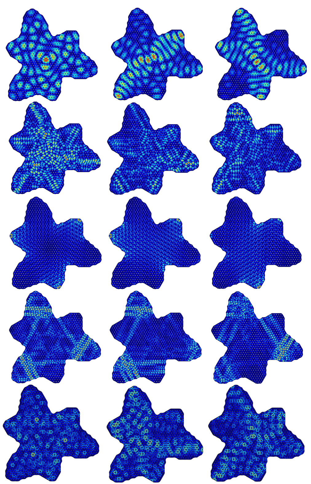
In Fig. 12 we show typical intensity distributions of the electric field strength of the DB and of the wave functions of the corresponding GB in Fig. 13. Examples are shown for the region below the flat band for singlets (first column) and corresponding doublets (second and third comlumn), from top to bottom, around the lower BE (first row), around the lower VHS (second row), around the DP (third row), around the upper VHS (fourth row) and for the DB also in the region of FB (fifth row). The wave functions of the doublet partners are superpositions of the corresponding symmetry-projected states with , and thus their intensity distributions exhibit different patterns. Around the BE, the intensity distributions are mostly spread over the whole billiard domain, some are localized around shortest periodic orbits, e.g., the connected one is shown in Fig. 4, whereas around the VHS we observe especially for the upper VHS a strong localization around periodic orbits in the bulges of the billiard. Accordingly we observe deviations from RMT predictions in the corresponding -matrix amplitude distributions for the middle and outer antenna groups, whereas good agreement is found when using power-law banded random matrices in Eq. (3). Note, that the amplitudes of the resonances depend on the electric-field strength at the position of the measuring antennas, and their distributions are obtained from averaging over all symmetry classes.

At the DP the resonances are well isolated. Therefore, in that region we can obtain information on the properties of the wave-function components in terms of the strength distribution Dembowski et al. 2005. Namely, for sufficiently isolated resonances the -matrix has the form
| (15) |
close to the th resonance frequency with denoting the total width of the corresponding resonance Alt et al. 1995. The partial widths and are proportional to the electric-field intensities at antennas and . They cannot be determined individually, however, the strengths may be obtained with high precision by fitting this expression to the resonances Dembowski et al. 2005. The strength distribution corresponds to the distribution of the products of the squared moduli of two wave-function components in the DB, or of two eigenvector components for the associated RMT model Dietz et al. 2006; Guhr et al. 1998. For 3GUE it coincides with that of GUE, , that of GOE+2GUE is given by , where . Here, denotes the modified Bessel function of order zero. In Fig. 11 (e) we compare these analytical expresssions to the distributions obtained for the DB in the Dirac region (red triangles). However, like for the FB we find only agreement with the RMT distributions, when using the corresponding PLBM , where that for GOE+2GUE (violet diamonds) is better than that for 3GUE (orange dashed-dotted lines).
VI Conclusions
We performed experiments with a superconducting DB, whose shape has a symmetry. To identify the resonance frequencies and to separate them into the three symmetry classes we successfully employed a procedure, which was originally developed for hollow microwave billiards Dembowski et al. 2003, thereby demonstrating that it is applicable even to complex structures like the DB. We confirm results which were obtained in Ref. Zhang and Dietz 2021 from numerical computations, namely, find good agreement of the spectral properties with those of the QB, GB and HKB of corresponding shape, and with those of massive relativistic NBs only beyond a certain mass. We also investigated properties of the wave functions below the DP1, where the DOS is low, in terms of the strength distribution. We find good agreement with the corresponding distributions of random matrices from GOE+2GUE when using PLBMs, corroborating that the wave functions are localized Bittner et al. 2012. Yet, the spectral properties of the associated resonance frequencies agree well with those of typical quantum systems with a symmetry and a chaotic classical dynamics. Furthermore, we for the first time investigated the fluctuation properties of the measured matrix in the regions around the BEs, the VHSs and the FB, which are not accessible numerically. In the nonrelativistic regime we find good agreement with those of the RMT model Eq. (14) for GOE+2GUE, whereas for the other regions we took account of the localization observed in parts of the DB by using PLBMs. Around the VHSs the ratio distributions agree well with those of random matrices from the GOE+2GUE. From these observations we may conclude that even in regions, where the wave functions are localized in parts of the DB, the spectral properties comply with those of typical quantum systems whose corresponding classical dynamics is chaotic Dietz et al. 2016.
VII Acknowledgement
This work was supported by the NSF of China under Grant Nos. 11775100, 12047501 and 11961131009. WZ acknowledges financial support from the China Scholarship Council (No. CSC-202106180044). BD and WZ acknowledge financial support from the Institute for Basic Science in Korea through the project IBS-R024-D1.
References
- Dietz et al. (2015a) B. Dietz, T. Klaus, M. Miski-Oglu, and A. Richter, Phys. Rev. B 91, 035411 (2015a).
- Bittner et al. (2010) S. Bittner, B. Dietz, M. Miski-Oglu, P. Oria Iriarte, A. Richter, and F. Schäfer, Phys. Rev. B 82, 014301 (2010).
- Bittner et al. (2012) S. Bittner, B. Dietz, M. Miski-Oglu, and A. Richter, Phys. Rev. B 85, 064301 (2012).
- Dietz et al. (2013) B. Dietz, F. Iachello, M. Miski-Oglu, N. Pietralla, A. Richter, L. von Smekal, and J. Wambach, Phys. Rev. B 88, 104101 (2013).
- Iachello et al. (2015) F. Iachello, B. Dietz, M. Miski-Oglu, and A. Richter, Phys. Rev. B 91, 214307 (2015).
- Dietz and Richter (2015) B. Dietz and A. Richter, Chaos 25, 097601 (2015).
- Dietz et al. (2015b) B. Dietz, T. Klaus, M. Miski-Oglu, A. Richter, M. Bischoff, L. von Smekal, and J. Wambach, Phys. Rev. Lett. 115, 026801 (2015b).
- Dietz et al. (2016) B. Dietz, T. Klaus, M. Miski-Oglu, A. Richter, M. Wunderle, and C. Bouazza, Phys. Rev. Lett. 116, 023901 (2016).
- Dietz and Richter (2019) B. Dietz and A. Richter, Phys. Scr. 94, 014002 (2019).
- Kuhl et al. (2010) U. Kuhl, S. Barkhofen, T. Tudorovskiy, H.-J. Stöckmann, T. Hossain, L. de Forges de Parny, and F. Mortessagne, Phys. Rev. B 82, 094308 (2010).
- Jacqmin et al. (2014) T. Jacqmin, I. Carusotto, I. Sagnes, M. Abbarchi, D. D. Solnyshkov, G. Malpuech, E. Galopin, A. Lemaître, J. Bloch, and A. Amo, Phys. Rev. Lett. 112, 116402 (2014).
- Lan et al. (2012) Z. Lan, N. Goldman, and P. Öhberg, Phys. Rev. B 85, 155451 (2012).
- Lu et al. (2017a) J.-L. Lu, W. Luo, X.-Y. Li, S.-Q. Yang, J.-X. Cao, X.-G. Gong, and H.-J. Xiang, Chinese Physics Letters 34, 057302 (2017a).
- Zhong et al. (2017) H. Zhong, Y. Zhang, Y. Zhu, D. Zhang, C. Li, Y. Zhang, F. Li, M. R. Belić, and M. Xiao, Annalen der Physik 529, 1600258 (2017).
- Maimaiti et al. (2020) W. Maimaiti, B. Dietz, and A. Andreanov, Phys. Rev. B 102, 214301 (2020).
- Zhang and Dietz (2021) W. Zhang and B. Dietz, Phys. Rev. B 104, 064310 (2021).
- Novoselov et al. (2004) K. S. Novoselov, A. K. Geim, S. V. Morozov, D. Jiang, Y. Zhang, S. V. Dubonos, I. V. Grigorieva, and A. A. Firsov, Science 306, 666 (2004).
- Beenakker (2008) C. W. J. Beenakker, Rev. Mod. Phys. 80, 1337 (2008).
- Castro Neto et al. (2009) A. H. Castro Neto, F. Guinea, N. M. R. Peres, K. S. Novoselov, and A. K. Geim, Rev. Mod. Phys. 81, 109 (2009).
- DiVincenzo and Mele (1984) D. P. DiVincenzo and E. J. Mele, Phys. Rev. B 29, 1685 (1984).
- Geim and Novoselov (2007) A. Geim and K. Novoselov, Nature Materials 6, 183 (2007).
- Avouris et al. (2007) P. Avouris, Z. Chen, and V. Perebeinos, Nat. Nanotech. 2, 605 (2007).
- Miao et al. (2007) F. Miao, S. Wijeratne, Y. Zhang, U. C. Coskun, W. Bao, and C. N. Lau, Science 317, 1530 (2007).
- Ponomarenko et al. (2008) L. A. Ponomarenko, F. Schedin, M. I. Katsnelson, R. Yang, E. W. Hill, K. S. Novoselov, and A. K. Geim, Science 320, 5874 (2008).
- Zhang and Liu (2008) X. Zhang and Z. Liu, Phys. Rev. Lett. 101, 264303 (2008).
- Abergel et al. (2010) D. Abergel, V. Apalkov, J. Berashevich, K. Ziegler, and T. Chakraborty, Adv. Phys. 59, 261 (2010).
- Zandbergen and de Dood (2010) S. R. Zandbergen and M. J. A. de Dood, Phys. Rev. Lett. 104, 043903 (2010).
- Polini et al. (2013) M. Polini, F. Guinea, M. Lewenstein, H. C. Manoharan, and V. Pellegrini, Nat. Nanotechnol. 8, 625 (2013).
- Parimi et al. (2004) P. V. Parimi, W. T. Lu, P. Vodo, J. Sokoloff, J. S. Derov, and S. Sridhar, Phys. Rev. Lett. 92, 127401 (2004).
- Joannopoulos et al. (2008) S. Joannopoulos, J. D. Johnson, R. Meade, and J. Winn, Photonic Crystals. Molding the Flow of Light (Princeton University Press, Princeton and Oxford, 2008).
- Singha et al. (2011) A. Singha, M. Gibertini, B. Karmakar, S. Yuan, M. Polini, G. Vignale, M. I. Katsnelson, A. Pinczuk, L. N. Pfeiffer, K. W. West, and V. Pellegrini, Science 332, 1176 (2011).
- Nádvorník et al. (2012) L. Nádvorník, M. Orlita, N. A. Goncharuk, L Smrčka, V. Novák, V. Jurka, K. Hruška, Z. Výborný, Z. R. Wasilewski, M. Potemski, and K. Výborný, New J. Phys. 14, 053002 (2012).
- Gomes et al. (2012) K. K. Gomes, W. Mar, W. Ko, F. Guinea, and H. C. Manoharan, Nature 483, 306 (2012).
- Tarruell et al. (2012) L. Tarruell, D. Greif, T. Uehlinger, G. Jotzu, and T. Esslinger, Nature 483, 302 (2012).
- Uehlinger et al. (2013) T. Uehlinger, G. Jotzu, M. Messer, D. Greif, W. Hofstetter, U. Bissbort, and T. Esslinger, Phys. Rev. Lett. 111, 185307 (2013).
- Rechtsman et al. (2013a) M. C. Rechtsman, Y. Plotnik, J. M. Zeuner, D. Song, Z. Chen, A. Szameit, and M. Segev, Phys. Rev. Lett. 111, 103901 (2013a).
- Rechtsman et al. (2013b) M. C. Rechtsman, J. M. Zeuner, A. Tünnermann, S. Nolte, M. Segev, and A. Szameit, Nat. Phot. 7, 153 (2013b).
- Khanikaev et al. (2013) A. B. Khanikaev, S. H. Mousavi, W.-K. Tse, M. Kargarian, A. H. MacDonald, and G. Shvets, Nat. Mater. 12, 233 (2013).
- Wang et al. (2014) X. Wang, H. T. Jiang, C. Yan, F. S. Deng, Y. Sun, Y. H. Li, Y. L. Shi, and H. Chen, EPL (Europhysics Letters) 108, 14002 (2014).
- Shi et al. (2015) Z. Shi, G. Lin, T.-H. Xiao, H.-L. Guo, , and Z.-Y. Li, Photonics 2, 1513 (2015).
- Bellec et al. (2013a) M. Bellec, U. Kuhl, G. Montambaux, and F. Mortessagne, Phys. Rev. Lett. 110, 033902 (2013a).
- Bellec et al. (2013b) M. Bellec, U. Kuhl, G. Montambaux, and F. Mortessagne, Phys. Rev. B 88, 115437 (2013b).
- Bellec et al. (2014) M. Bellec, U. Kuhl, G. Montambaux, and F. Mortessagne, New J. Phys. 16, 113023 (2014).
- Dembowski et al. (2000) C. Dembowski, H.-D. Gräf, A. Heine, H. Rehfeld, A. Richter, and C. Schmit, Phys. Rev. E 62, R4516 (2000).
- Berry and Tabor (1977) M. V. Berry and M. Tabor, J. Phys. A 10, 371 (1977).
- Berry (1979) M. Berry, Structural Stability in Physics (Pergamon Press, Berlin, 1979).
- Casati et al. (1980) G. Casati, F. Valz-Gris, and I. Guarnieri, Lett. Nuovo Cimento 28, 279 (1980).
- Bohigas et al. (1984) O. Bohigas, M. J. Giannoni, and C. Schmit, Phys. Rev. Lett. 52, 1 (1984).
- Leyvraz et al. (1996) F. Leyvraz, C. Schmit, and T. H. Seligman, J. Phys. A 29, L575 (1996).
- Dembowski et al. (2003) C. Dembowski, B. Dietz, H.-D. Gräf, A. Heine, F. Leyvraz, M. Miski-Oglu, A. Richter, and T. H. Seligman, Phys. Rev. Lett. 90, 014102 (2003).
- Knill (1998) O. Knill, Elemente der Mathematik 53, 89 (1998).
- Gutkin (2007) B. Gutkin, J. Phys. A 40, F761 (2007).
- Veble et al. (2007) G. Veble, T. Prosen, and M. Robnik, New J. Phys. 9, 15 (2007).
- Dietz et al. (2014) B. Dietz, T. Guhr, B. Gutkin, M. Miski-Oglu, and A. Richter, Phys. Rev. E 90, 022903 (2014).
- Rego et al. (2005) L. G. C. Rego, A. Gusso, and M. G. E. da Luz, Journal of Physics A: Mathematical and General 38, L639 (2005).
- Gusso et al. (2006) A. Gusso, M. G. E. da Luz, and L. G. C. Rego, Phys. Rev. B 73, 035436 (2006).
- Robbins (1989a) J. M. Robbins, Phys. Rev. A 40, 2128 (1989a).
- Keating and Robbins (1997) J. P. Keating and J. M. Robbins, J. Phys. A 30, L177 (1997).
- Joyner et al. (2012) C. H. Joyner, S. Müller, and M. Sieber, J. Phys. A 45, 205102 (2012).
- Wallace (1947) P. R. Wallace, Phys. Rev. 71, 622 (1947).
- Berry and Mondragon (1987) M. V. Berry and R. J. Mondragon, Proc. R. Soc. London A 412, 53 (1987).
- Weyl (1929) H. Weyl, Z. Physik 56, 330 (1929).
- Yu et al. (2016) P. Yu, Z.-Y. Li, H.-Y. Xu, L. Huang, B. Dietz, C. Grebogi, and Y.-C. Lai, Phys. Rev. E 94, 062214 (2016).
- Yu et al. (2022) P. Yu, W. Zhang, B. Dietz, and L. Huang, Journal of Physics A: Mathematical and Theoretical 55, 224015 (2022).
- Silvestrov and Efetov (2007) P. G. Silvestrov and K. B. Efetov, Phys. Rev. Lett. 98, 016802 (2007).
- Libisch et al. (2009) F. Libisch, C. Stampfer, and J. Burgdörfer, Phys. Rev. B 79, 115423 (2009).
- Wurm et al. (2009) J. Wurm, A. Rycerz, İ. Adagideli, M. Wimmer, K. Richter, and H. U. Baranger, Phys. Rev. Lett. 102, 056806 (2009).
- Huang et al. (2010) L. Huang, Y.-C. Lai, and C. Grebogi, Phys. Rev. E 81, 055203 (R) (2010).
- Wurm et al. (2011) J. Wurm, K. Richter, and İ. Adagideli, Phys. Rev. B 84, 075468 (2011).
- Rycerz (2012) A. Rycerz, Phys. Rev. B 85, 245424 (2012).
- Rycerz (2013) A. Rycerz, Phys. Rev. B 87, 195431 (2013).
- Albeverio et al. (1996) S. Albeverio, F. Haake, P. Kurasov, M. Kuś, and P. Šeba, J. Math. Phys. 37, 4888 (1996).
- Dembowski et al. (2005) C. Dembowski, B. Dietz, T. Friedrich, H.-D. Gräf, H. L. Harney, A. Heine, M. Miski-Oglu, and A. Richter, Phys. Rev. E 71, 046202 (2005).
- Dietz et al. (2006) B. Dietz, T. Guhr, H. L. Harney, and A. Richter, Phys. Rev. Lett. 96, 254101 (2006).
- Stöckmann and Stein (1990) H.-J. Stöckmann and J. Stein, Phys. Rev. Lett. 64, 2215 (1990).
- Sridhar (1991) S. Sridhar, Phys. Rev. Lett. 67, 785 (1991).
- Gräf et al. (1992) H.-D. Gräf, H. L. Harney, H. Lengeler, C. H. Lewenkopf, C. Rangacharyulu, A. Richter, P. Schardt, and H. A. Weidenmüller, Phys. Rev. Lett. 69, 1296 (1992).
- Haake et al. (2018) F. Haake, S. Gnutzmann, and M. Kuś, Quantum Signatures of Chaos (Springer-Verlag, Heidelberg, 2018).
- Dietz and Li (2020) B. Dietz and Z.-Y. Li, Phys. Rev. E 102, 042214 (2020).
- Baym (2018) G. Baym, Lectures on Quantum Mechanics (CRC Press, Boca Raton, FL, 2018).
- Dietz (2021) B. Dietz, Act. Phys. Pol. A 140, 473 (2021).
- Bäcker (2003) A. Bäcker, Numerical Aspects of Eigenvalue and Eigenfunction Computations for Chaotic Quantum Systems (Springer Berlin Heidelberg, Berlin, Heidelberg, 2003), pp. 91–144.
- Dietz (2022) B. Dietz, J. Phys. A: Math. Theor. 55, 474003 (2022).
- Keating and Robbins (1996) J. P. Keating and J. M. Robbins, J. Phys. A: Math. Gen. 30, L177 (1996).
- Braun et al. (2011) P. Braun, F. Leyvraz, and T. H. Seligman, New J. Phys. 13, 063027 (2011).
- Schäfer et al. (2002) R. Schäfer, M. Barth, F. Leyvraz, M. Müller, T. H. Seligman, and H.-J. Stöckmann, Phys. Rev. E 66, 016202 (2002).
- Robbins (1989b) J. M. Robbins, Phys. Rev. A 40, 2128 (1989b).
- Seligman and Weidenmüller (1994) T. H. Seligman and H. A. Weidenmüller, J. Phys. A 27, 7915 (1994).
- Lu et al. (2014) J. Lu, C. Qiu, S. Xu, Y. Ye, M. Ke, and Z. Liu, Phys. Rev. B 89, 134302 (2014).
- Lu et al. (2016) J. Lu, C. Qiu, M. Ke, and Z. Liu, Phys. Rev. Lett. 116, 093901 (2016).
- Lu et al. (2017b) J. Lu, C. Qiu, L. Ye, X. Fan, M. Ke, F. Zhang, and Z. Liu, Nat. Phys. 13, 369 (2017b).
- Ye et al. (2017) L. Ye, C. Qiu, J. Lu, X. Wen, Y. Shen, M. Ke, F. Zhang, and Z. Liu, Phys. Rev. B 95, 174106 (2017).
- Xia et al. (2017) B.-Z. Xia, T.-T. Liu, G.-L. Huang, H.-Q. Dai, J.-R. Jiao, X.-G. Zang, D.-J. Yu, S.-J. Zheng, and J. Liu, Phys. Rev. B 96, 094106 (2017).
- Dietz et al. (2008) B. Dietz, T. Friedrich, H. L. Harney, M. Miski-Oglu, A. Richter, F. Schäfer, and H. A. Weidenmüller, Phys. Rev. E 78, 055204 (2008).
- Dietz et al. (2009) B. Dietz, T. Friedrich, H. L. Harney, M. Miski-Oglu, A. Richter, F. Schäfer, J. Verbaarschot, and H. A. Weidenmüller, Phys. Rev. Lett. 103, 064101 (2009).
- Dietz et al. (2010) B. Dietz, T. Friedrich, H. L. Harney, M. Miski-Oglu, A. Richter, F. Schäfer, and H. A. Weidenmüller, Phys. Rev. E 81, 036205 (2010).
- Reich et al. (2002) S. Reich, J. Maultzsch, C. Thomsen, and P. Ordejón, Phys. Rev. B 66, 035412 (2002).
- Bohigas and Giannoni (1974) O. Bohigas and M. J. Giannoni, Ann. Phys. 89, 393 (1974).
- Mehta (2004) M. L. Mehta, Random Matrices (Elsevier, Amsterdam, 2004).
- Oganesyan and Huse (2007) V. Oganesyan and D. A. Huse, Phys. Rev. B 75, 155111 (2007).
- Atas et al. (2013) Y. Y. Atas, E. Bogomolny, O. Giraud, and G. Roux, Phys. Rev. Lett. 110, 084101 (2013).
- Mahaux and Weidenmüller (1969) C. Mahaux and H. A. Weidenmüller, Shell Model Approach to Nuclear Reactions (North Holland, Amsterdam, 1969).
- Verbaarschot et al. (1985) J. Verbaarschot, H. Weidenmüller, and M. Zirnbauer, Phys. Rep. 129, 367 (1985).
- Mirlin et al. (1996) A. D. Mirlin, Y. V. Fyodorov, F.-M. Dittes, J. Quezada, and T. H. Seligman, Phys. Rev. E 54, 3221 (1996).
- Alt et al. (1995) H. Alt, H. D. Gräf, H. L. Harney, R. Hofferbert, H. Lengeler, A. Richter, P. Schardt, and H. A. Weidenmüller, Phys. Rev. Lett. 74, 62 (1995).
- Guhr et al. (1998) T. Guhr, A. Müller-Groeling, and H. A. Weidenmüller, Phys. Rep. 299, 189 (1998).