Exact Renormalization Group in Large $N$ Preprint: KOBE-TH-23-02

Hidenori SONODA Email: hsonoda@kobe-u.ac.jp Affiliation: Physics Department, Kobe University, Kobe 657-8501, Japan

22 February 2023

Abstract

We apply the exact renormalization group formalism to compute the effective action and potential of the four dimensional O $(N)$ linear sigma model in large $N$ . With a finite momentum cutoff in place, the model is well defined. In the naive continuum limit where the cutoff is taken to infinity, the effective action suffers from a tachyon, and the effective potential is unbounded from below and develops a negative imaginary part. These problems disappear once a small enough cutoff is restored. The effective potential of the naive continuum limit, obtained by analytic continuation, is given explicitly in terms of the Lambert $W$ function.

Keywords:

exact renormalization groups, Large N, cutoffs, effective potentials, tachyons, instability, Lambert W function

I Introduction

The large $N$ approximation was first introduced for the spherical model Berlin and Kac 1952 on a lattice by Berlin and Kac. The model that imposes a global constraint on the size of the spins turned out to be equivalent to the O $(N)$ non-linear sigma model in large $N$ Stanley 1968. The large $N$ approximation, being consistent with scaling, has been an essential tool for our understanding of critical phenomena. (See Ma Ma 1973 for review.)

The approximation was first introduced to quantum field theory in Wilson 1973. With the hope that physics, at least qualitatively, does not depend much on $N$ , it has become a popular exercise to study the large $N$ limit. (See Moshe and Zinn-Justin 2003 for a review of the early works in large $N$ .) The subject of this paper is the four dimensional O $(N)$ linear sigma model in large $N$ , which was first studied in Dolan and Jackiw 1974; Schnitzer 1974a; Schnitzer 1974b; Coleman et al. 1974.

We have set two purposes for the paper:

1.

The malaise of the large $N$ limit in four dimensions found in Coleman et al. 1974 is pursued further.
2.

The technique of the exact renormalization group (ERG, for short) is used for the calculations of the effective action and potential.

In Coleman et al. 1974 two main problems were discovered: (a) the effective potential $V_{\mathrm{eff}}(\varphi)$ ( $\varphi$ will be defined precisely in Sec. II) can be defined only up to a maximum $\varphi_{\max}$ beyond which the potential becomes complex, (b) the effective action suffers from tachyon poles. We will confirm both problems. As for (a), we give an analytic expression for $V_{\mathrm{eff}}(\varphi)$ in terms of the Lambert $W$ function Corless et al. 1996; Wikipedia 2023. This has actually been done already in Sonoda 2013, but we go one step further here. We extend $V_{\mathrm{eff}}(\varphi)$ beyond $\varphi_{\max}$ by analytic continuation. As argued in Coleman et al. 1974, the potential is complex for $\varphi>\varphi_{\max}$ . But our finding is contrary to the expectation of Coleman et al. 1974 that there may be a true minimum beyond $\varphi_{\max}$ . We find that the real part of the potential is unbounded from below. We will show that both (a) and (b) go away if the momentum cutoff $\Lambda_{0}$ is kept finite, agreeing with the observations made in Sec. III of Sonoda 2013.

The second purpose of the paper is to demonstrate that both the effective action and the effective potential can be calculated by integrating the ERG differential equation for the Wilson action. ERG was first introduced in sect. 11 of Wilson and Kogut 1974. Given a theory with momentum cutoff $\Lambda_{0}$ we integrate over the fields with momenta below $\Lambda_{0}$ all the way to zero. In the ERG formalism we do the integration incrementally scale by scale by solving the ERG differential equation. The ERG formalism has been actively pursued from the 1990’s, and by now many reviews are available. (See Morris 1994; Becchi 1996; Berges et al. 2002; Pawlowski 2007; Gies 2012; Igarashi et al. 2010; Rosten 2012; Dupuis et al. 2021 among others.) Yet, to introduce our notation, we will start our paper with a short overview of the formalism.

The paper is organized as follows. In Sec. II we overview the ERG formalism, and explain the simplification obtained in large $N$ . In Sec. III, we give a general solution to the ERG differential equation derived in the previous section. In Sec. IV, we explain that the ERG differential equation has no nontrivial fixed-point solution. This implies that there is no interacting continuum limit, but as an alternative we introduce a “naive continuum limit” to be studied in the following sections. In Sec. V, we compute the effective action of the naive continuum limit, and confirm the presence of a tachyon which was first observed in Coleman et al. 1974. Then, in Sec. VI, we compute the corresponding effective potential $V_{\mathrm{eff}}(\varphi)$ . The effective potential, defined only up to a maximum field $\varphi_{\max}$ , can be given an analytic form in terms of the Lambert $W$ function Corless et al. 1996; Wikipedia 2023, as was shown already in Sonoda 2013. We can continue $V_{\mathrm{eff}}(\varphi)$ analytically beyond $\varphi_{\max}$ but find that the potential develops a negative imaginary part, and that its real part is unbounded from below. In Sec. VII, we replace the naive continuum limit by a theory with a bare cutoff $\Lambda_{0}$ . By using the general solution of the ERG differential equation given in Sec. III, we construct both the effective action and the effective potential. The effective action is free from tachyons. The effective potential agrees with the naive continuum limit for small fields, but approaches the bare potential for large fields. In Sec. VIII, we compare the naive continuum limit with the bare theory. We observe how a bound state is converted to a tachyon as we raise the cutoff beyond the allowed maximum, the Landau pole. In IX we give concluding remarks. We have prepared five appendices to give details omitted in the main text.

All through the paper we work in the momentum space and use the shorthand notation

\int_{p}\equiv\int\frac{d^{D}p}{(2\pi)^{D}},\quad\delta(p)\equiv(2\pi)^{D}\delta^{(D)}(p)\,.

II Short overview of the ERG formalism

We consider a Wilson action $S_{t}[\phi]$ for the O $(N)$ linear sigma model consisting of a real scalar field $\phi^{I}$ ( $I=1,\cdots,N$ ) with $N$ components (we use Einstein’s convention for repeated indices). It satisfies the differential equation

	$\displaystyle\partial_{t}e^{S_{t}[\phi]}$	$\displaystyle=\int_{p}\Bigg[\left(-p\cdot\partial_{p}\ln K(p)+\frac{D+2}{2}-\gamma_{t}+p\cdot\partial_{p}\right)\phi^{I}(p)\cdot\frac{\delta}{\delta\phi^{I}(p)}$
		$\displaystyle\quad+\left(-p\cdot\partial_{p}\ln R(p)+2-2\gamma_{t}\right)\frac{K(p)^{2}}{R(p)}\frac{1}{2}\frac{\delta^{2}}{\delta\phi^{I}(p)\phi^{I}(-p)}\Bigg]e^{S_{t}[\phi]}\,,$		(1)

where $K$ and $R$ are two independent momentum cutoff functions, both of which are decreasing positive functions of $p^{2}$ , are $1$ at $p=0$ , and vanish rapidly as $p^{2}\to\infty$ Sonoda 2015. We denote the usual correlation functions using single brackets:¹¹ 1 Please note our sign convention for the Wilson action. The Boltzmann weight is $e^{S_{t}}$ , not $e^{-S_{t}}$ .

\left\langle\cdots\right\rangle_{S_{t}}\equiv\int[d\phi]\,e^{S_{t}[\phi]}\,\cdots\,.

(2)

The $t$ -dependence (1) of the Wilson action is determined so that the correlation functions, modified as Sonoda 2015

		$\displaystyle\left\langle\kern-3.00003pt\left\langle\phi^{I_{1}}(p_{1})\cdots\phi^{I_{n}}(p_{n})\right\rangle\kern-3.00003pt\right\rangle_{t}$
		$\displaystyle\equiv\prod_{i=1}^{n}\frac{1}{K(p_{i})}\cdot\left\langle\exp\left(-\int_{p}\frac{K(p)^{2}}{R(p)}\frac{1}{2}\frac{\delta^{2}}{\delta\phi^{I}(p)\delta\phi^{I}(-p)}\right)\phi^{I_{1}}(p_{1})\cdots\phi^{I_{n}}(p_{n})\right\rangle_{S_{t}}\,,$		(3)

satisfy the scaling relations

		$\displaystyle\left\langle\kern-3.00003pt\left\langle\phi^{I_{1}}(p_{1}e^{t-t^{\prime}})\cdots\phi^{I_{n}}(p_{n}e^{t-t^{\prime}})\right\rangle\kern-3.00003pt\right\rangle_{t}$
		$\displaystyle=\exp\left[n\left(-\frac{D+2}{2}(t-t^{\prime})+\int_{t^{\prime}}^{t}ds\,\gamma_{s}\right)\right]\cdot\left\langle\kern-3.00003pt\left\langle\phi^{I_{1}}(p_{1})\cdots\phi^{I_{n}}(p_{n})\right\rangle\kern-3.00003pt\right\rangle_{t^{\prime}}\,.$		(4)

Clearly, $\gamma_{t}$ gives the scale dependent anomalous dimension of $\phi^{I}$ .

To define the one-particle-irreducible (1PI) part of the Wilson action, it is convenient first to define a generating functional with an IR cutoff by

W_{t}[J]\equiv S_{t}[\phi]+\frac{1}{2}\int_{p}\frac{J^{I}(p)J^{I}(-p)}{R(p)}\,,

(5)

where

J^{I}(p)\equiv\phi^{I}(p)\frac{R(p)}{K(p)}\,.

(6)

The cutoff function $R(p)$ provides an IR cutoff of order $1$ because the momenta below the cutoff has not been integrated yet. Eq. (1) for $S_{t}$ implies

	$\displaystyle\partial_{t}e^{W_{t}[J]}$	$\displaystyle=\int_{p}\Bigg[\left(p\cdot\partial_{p}+\frac{D-2}{2}+\gamma_{t}\right)J^{I}(p)\cdot\frac{\delta}{\delta J^{I}(p)}$
		$\displaystyle\quad+\left(-p\cdot\partial_{p}+2-2\gamma_{t}\right)R(p)\cdot\frac{1}{2}\frac{\delta^{2}}{\delta J^{I}(p)\delta J^{I}(-p)}\Bigg]\,e^{W_{t}[J]}\,,$		(7)

which is simpler than Eq. (1) in that it depends only on the cutoff function $R(p)$ , but not on $K(p)$ .

We can now define the 1PI Wilson action $\Gamma_{t}[\Phi]$ as the Legendre transform of $W_{t}[J]$ by

\Gamma_{t}[\Phi]-\frac{1}{2}\int_{p}R(p)\Phi^{I}(p)\Phi^{I}(-p)\equiv W_{t}[J]-\int_{p}J^{I}(-p)\Phi^{I}(p)\,,

(8)

where we define

\Phi^{I}(p)\equiv\frac{\delta W[J]}{\delta J^{I}(-p)}\,.

(9)

Differentiating (8) with respect to $\Phi^{I}$ , we obtain

J^{I}(p)=R(p)\Phi^{I}(p)-\frac{\delta\Gamma_{t}[\Phi]}{\delta J^{I}(-p)}\,.

(10)

From Eq. (7) we obtain the ERG equation for $\Gamma_{t}[\Phi]$ as²² 2 This equation is known as the Wetterich equation. It is introduced and popularized in Wetterich 1993.

	$\displaystyle\partial_{t}\Gamma_{t}[\Phi]$	$\displaystyle=\int_{p}\left(p\cdot\partial_{p}+\frac{D+2}{2}-\gamma_{t}\right)\Phi^{I}(p)\cdot\frac{\delta\Gamma_{t}[\Phi]}{\delta\Phi^{I}(p)}$
		$\displaystyle\quad+\int_{p}\left(-p\cdot\partial_{p}+2-2\gamma_{t}\right)R(p)\cdot\frac{1}{2}\mathcal{G}_{t;p,-p}^{II}[\Phi]\,,$		(11)

where

\displaystyle\mathcal{G}_{t;p,-q}^{IJ}[\Phi]\equiv\frac{\delta^{2}W_{t}[J]}{\delta J^{I}(p)\delta J^{J}(-q)}

(12)

is determined by the differential equation

\displaystyle\int_{q}\mathcal{G}_{t;p,-q}^{IJ}[\Phi]\left(R(q)\delta^{JK}\delta(q-r)-\frac{\delta^{2}\Gamma_{t}[\Phi]}{\delta\Phi^{J}(q)\delta\Phi^{K}(-r)}\right)=\delta^{IK}\delta(p-r)\,.

(13)

Let us now introduce the large $N$ approximation following D’Attanasio and Morris 1997. We first split $\Gamma_{t}$ into the Gaussian and interaction parts

\Gamma_{t}[\Phi]=-\frac{1}{2}\int_{p}p^{2}\Phi^{I}(p)\Phi^{I}(-p)+N\Gamma_{I,t}[\varphi]\,,

(14)

and then assume that the interaction part is a functional of

\varphi(p)\equiv\frac{1}{2N}\int_{q}\Phi^{I}(q+p)\Phi^{I}(-q)\,.

(15)

Since the interaction part has no kinetic term, the assumption (14) implies the vanishing anomalous dimension

\gamma_{t}=0\,.

(16)

Let us verify the consistency of this approximation in the large $N$ limit. Substitution of (15) gives

\int_{p}\left(p\cdot\partial_{p}+\frac{D+2}{2}\right)\Phi^{I}(p)\cdot\frac{\delta\Gamma_{I,t}[\varphi]}{\delta\Phi^{I}(p)}=\int_{p}\left(2+p\cdot\partial_{p}\right)\varphi(p)\cdot\frac{\delta\Gamma_{I,t}[\varphi]}{\delta\varphi(p)}\,.

Since we can approximate

$\displaystyle N\frac{\delta^{2}\Gamma_{I,t}[\varphi]}{\delta\Phi^{J}(q)\delta\Phi^{K}(-r)}$	$\displaystyle=\frac{\delta}{\delta\Phi^{J}(q)}\int_{s}\Phi^{K}(s+r)\frac{\delta\Gamma_{I,t}[\varphi]}{\delta\varphi(s)}$
	$\displaystyle=\delta^{JK}\frac{\delta\Gamma_{I,t}[\varphi]}{\delta\varphi(q-r)}+\int_{s,t}\frac{1}{N}\Phi^{K}(s+r)\Phi^{J}(t-q)\frac{\delta^{2}\Gamma_{I,t}[\varphi]}{\delta\varphi(s)\delta\varphi(t)}$
	$\displaystyle\overset{N\gg 1}{\longrightarrow}\delta^{JK}\frac{\delta\Gamma_{I,t}[\varphi]}{\delta\varphi(q-r)}$	(17)

for large $N$ , we obtain

\mathcal{G}^{IJ}_{t;p,-q}[\Phi]\overset{N\gg 1}{\longrightarrow}\delta^{IJ}\mathcal{G}_{t;p,-q}[\varphi]\,,

(18)

where $\mathcal{G}_{t;p,-q}[\varphi]$ is a functional of $\varphi$ , defined by

\int_{q}\mathcal{G}_{t;p,-q}[\varphi]\left[\left(q^{2}+R(q)\right)\delta(q-r)-\frac{\delta\Gamma_{I,t}[\varphi]}{\delta\varphi(q-r)}\right]=\delta(p-r)\,.

(19)

Hence, for large $N$ , it is consistent to assume the structure (14), and we obtain the ERG equation for $\Gamma_{I,t}[\varphi]$ as

\partial_{t}\Gamma_{I,t}[\varphi]=\int_{p}(2+p\cdot\partial_{p})\varphi(p)\cdot\frac{\delta\Gamma_{I,t}[\varphi]}{\delta\varphi(p)}+\int_{p}(2-p\cdot\partial_{p})R(p)\cdot\frac{1}{2}\mathcal{G}_{t;p,-p}[\varphi]\,.

(20)

We will solve this in the next section.

Before proceeding to the next section, we would like to explain briefly the relation between $\Gamma_{I,t}[\varphi]$ and the physical effective action $\Gamma_{I,\mathrm{eff}}[\varphi]$ . $\Gamma_{I,t}[\varphi]$ is constructed in the dimensionless convention; all the physical quantities are dimensionless, measured in units of appropriate powers of the momentum cutoff. To restore physical dimensionful quantities, we introduce $\Lambda=\mu e^{-t}$ that corresponds to the physical momentum cutoff. This gives us an effective action $\Gamma_{I,\Lambda}[\varphi]$ in the dimensionful convention. The cutoff $\Lambda$ is an IR cutoff, since the fields with momenta less than $\Lambda$ have not been integrated out for the construction of $\Gamma_{I,\Lambda}[\varphi]$ . By taking $\Lambda\to 0+$ , we obtain the physical effective action $\Gamma_{I,\mathrm{eff}}[\varphi]$ which gives the 1PI correlation functions in the dimensionful convention Sonoda 2017. In general the limit depends on the finite momentum scale $\mu$ which plays the role of a renormalization scale. We give some details in Appendix A.

What about renormalizability of the theory? The theory is renormalizable if $\Gamma_{I,t}[\varphi]$ has a well defined limit as we take $t\to-\infty$ ; the limit is a UV fixed point of the ERG transformation. In four dimensions there is no fixed point, and the theory is not renormalizable in the strict sense. We discuss this in Sec. IV.

III Solving the ERG equation in $D=4$

To solve Eq. (20), we use a well known trick of the Legendre transformation, which has been used extensively for the studies of the effective potential in the large $N$ D’Attanasio and Morris 1997; Morris and Turner 1998; Litim and Trott 2018. We apply the same trick to the 1PI Wilson action.³³ 3 The same Legendre transformation was used in Coleman et al. 1974. The variable $\sigma$ in this paper corresponds to the auxiliary field $-\chi$ in Coleman et al. 1974. Eq. (2.6a) of Coleman et al. 1974 corresponds to our (23).

We introduce the Legendre transform $F_{t}[\sigma]$ by

\Gamma_{I,t}[\varphi]=F_{t}[\sigma]+\int_{p}\sigma(p)\varphi(-p)\,,

(21)

where

\sigma(p)=\frac{\delta\Gamma_{I,t}[\varphi]}{\delta\varphi(-p)}

(22)

so that we obtain

\varphi(p)=-\frac{\delta F_{t}[\sigma]}{\delta\sigma(-p)}\,.

(23)

Once we obtain $F_{t}[\sigma]$ , we can construct the corresponding $\Gamma_{I,t}[\varphi]$ by Eq. (21), where $\varphi$ is given by Eq. (23).

Now, the ERG equation for $F_{t}[\sigma]$ is given by

	$\displaystyle\partial_{t}F_{t}[\sigma]$	$\displaystyle=\partial_{t}\Gamma_{I,t}[\varphi]$
		$\displaystyle=\int_{p}\left(D-2+p\cdot\partial_{p}\right)\sigma(p)\cdot\frac{\delta F_{t}[\sigma]}{\delta\sigma(p)}+\int_{p}(2-p\cdot\partial_{p})R(p)\cdot\frac{1}{2}\mathcal{G}_{t;p,-p}[\varphi]\,,$		(24)

where Eq. (13) defines $\mathcal{G}_{t;p,-q}[\varphi]$ by

\int_{q}\mathcal{G}_{t;p,-q}[\varphi]\left[(q^{2}+R(q))\delta(q-r)-\sigma(-q+r)\right]=\delta(p-r)\,.

(25)

As a functional of $\sigma$ , $\mathcal{G}_{t;p,-q}[\varphi]$ has no explicit $t$ -dependence, and we will write

\mathcal{G}_{p,-q}[\sigma]=\mathcal{G}_{t;p,-q}[\varphi]

(26)

from now on.

Solving

\int_{q}\mathcal{G}_{p,-q}[\sigma]\left[(q^{2}+R(q))\delta(q-r)-\sigma(-q+r)\right]=\delta(p-r)

(27)

in powers of $\sigma$ , we obtain

		$\displaystyle\mathcal{G}_{p,-q}[\sigma]=h(p)\delta(p-q)$
		$\displaystyle\,+h(p)\left[\sigma(-p+q)+\int_{p_{1},p_{2}}\sigma(p_{1})h(p+p_{1})\sigma(p_{2})\delta(p_{1}+p_{2}+p-q)\right.$
		$\displaystyle\quad\left.+\int_{p_{1},p_{2},p_{3}}\sigma(p_{1})h(p+p_{1})\sigma(p_{2})h(p+p_{1}+p_{2})\sigma(p_{3})\delta(p_{1}+p_{2}+p_{3}+p-q)+\cdots\right]h(q)\,,$		(28)

where we define the high momentum propagator by

h(p)\equiv\frac{1}{p^{2}+R(p)}\,.

(29)

( $R(p)$ is of order $1$ for $p<1$ , but nearly zero for $p\gg 1$ .)

III.1 General solution for $D=4$

The general solution of Eq. (24) depends on $D$ , and we now specialize $D=4$ .⁴⁴ 4 For $2<D<4$ , there is a $t$ -independent particular solution $I[\sigma]$ that corresponds to the Wilson-Fisher fixed point. It is given by the sum of a particular solution $I_{t}[\sigma]$ and an arbitrary homogeneous solution:

F_{t}[\sigma]=I_{t}[\sigma]+\tilde{F}[\sigma_{-t}]\,.

(30)

We first explain the particular solution, which is given by

I_{t}[\sigma]=-\frac{1}{4}\int_{p}f(p)\,\sigma(0)+\frac{1}{2}\int_{p}\sigma(p)\sigma(-p)\left(\frac{t}{(4\pi)^{2}}+\mathcal{F}(p)\right)+I[\sigma]\,.

(31)

The functional $I[\sigma]$ , defined by

I[\sigma]\equiv\sum_{n=3}^{\infty}\frac{1}{2n}\int_{p_{1},\cdots,p_{n}}\sigma(p_{1})\cdots\sigma(p_{n})\,\delta\left(\sum_{1}^{n}p_{i}\right)\,I_{n}(p_{1},\cdots,p_{n})

(32)

and

I_{n\geq 3}(p_{1},\cdots,p_{n})\equiv\int_{q}h(q)h(q+p_{1})h(q+p_{1}+p_{2})\cdots h(q+p_{1}+\cdots+p_{n-1})\,,

(33)

satisfies the differential equation

		$\displaystyle\int_{p}\left(p\cdot\partial_{p}+2\right)\sigma(p)\cdot\frac{\delta I[\sigma]}{\delta\sigma(p)}=\frac{1}{2}\int_{p}(p\cdot\partial_{p}-2)R(p)\cdot\Big[\mathcal{G}_{p,-p}[\sigma]$
		$\displaystyle\qquad-h(p)\delta(0)-h(p)^{2}\sigma(0)-h(p)^{2}\int_{q}\sigma(q)h(p+q)\sigma(-q)\Big]\,.$		(34)

Note $I_{n\geq 3}$ is a convergent integral for $D=4$ , and it satisfies the differential equation

		$\displaystyle\left(\sum_{i}p_{i}\cdot\partial_{p_{i}}+2(n-2)\right)I_{n}(p_{1},\cdots,p_{n})$
		$\displaystyle=\int_{p}\Big(f(p)h(p+p_{1})\cdots h(p+\sum_{1}^{n-1}p_{i})+h(p)f(p+p_{1})\cdots h(p+\sum_{1}^{n-1}p_{i})$
		$\displaystyle\qquad+\cdots+h(p)h(p+p_{1})\cdots f(p+\sum_{1}^{n-1}p_{i})\Bigg)\,,$		(35)

where

f(p)\equiv\left(p\cdot\partial_{p}+2\right)h(p)=\frac{(2-p\cdot\partial_{p})R(p)}{\left(p^{2}+R(p)\right)^{2}}\,.

(36)

The function $\mathcal{F}(p)$ is determined by

p\cdot\partial_{p}\mathcal{F}(p)=\int_{q}f(q)\left(h(q+p)-h(q)\right)

(37)

and

\mathcal{F}(0)=0\,.

(38)

It is given explicitly by

\mathcal{F}(p)=\frac{1}{2}\int_{p}h(q)\left(h(q+p)-h(q)\right)\,.

(39)

Since

	$\displaystyle\int_{p}f(p)h(p)$	$\displaystyle=\int_{p}(p\cdot\partial_{p}-2)R(p)\cdot h(p)^{3}=\frac{1}{2}\int_{p}(p\cdot\partial_{p}+4)h(p)^{2}$
		$\displaystyle=\frac{1}{(4\pi)^{2}}\int_{0}^{\infty}dp^{2}\,\frac{d}{dp^{2}}\left(p^{4}h(p)^{2}\right)=\frac{1}{(4\pi)^{2}}\,,$		(40)

we can rewrite (37) as

p\cdot\partial_{p}\mathcal{F}(p)=\int_{q}f(q)h(q+p)-\frac{1}{(4\pi)^{2}}\,.

(41)

So much for the particular solution $I_{t}[\sigma]$ . (Please see Appendix B for more details on $I[\sigma]$ .)

The homogeneous solution $\tilde{F}[\sigma_{-t}]$ is an arbitrary functional of

\sigma_{-t}(p)\equiv e^{2t}\sigma(pe^{t})\,.

(42)

We find

\partial_{t}\tilde{F}[\sigma_{-t}]=\int_{p}\left(p\cdot\partial_{p}+2\right)\sigma(p)\cdot\frac{\delta\tilde{F}[\sigma_{-t}]}{\delta\sigma(p)}\,.

(43)

Expanding $\tilde{F}[\sigma]$ in powers of $\sigma$

\tilde{F}[\sigma]=f_{1}\sigma(0)+\sum_{n=2}^{\infty}\frac{1}{n!}\int_{p_{1},\cdots,p_{n}}\sigma(p_{1})\cdots\sigma(p_{n})\,\delta\left(\sum_{1}^{n}p_{i}\right)\,f_{n}(p_{1},\cdots,p_{n})\,,

(44)

we obtain

$\displaystyle\tilde{F}[\sigma_{-t}]$	$\displaystyle=f_{1}e^{2t}\sigma(0)+\frac{1}{2}\int_{p}\sigma(p)\sigma(-p)f_{2}(pe^{-t},-pe^{-t})$
	$\displaystyle\quad+\sum_{n=3}^{\infty}\frac{1}{n!}\int_{p_{1},\cdots,p_{n}}\sigma(p_{1})\cdots\sigma(p_{n})\,\delta\left(\sum_{1}^{n}p_{i}\right)\,e^{2(2-n)t}f_{n}(p_{1}e^{-t},\cdots,p_{n}e^{-t})$	(45)
	$\displaystyle\overset{t\to+\infty}{\longrightarrow}f_{1}e^{2t}\sigma(0)+f_{2}(0,0)\frac{1}{2}\int_{p}\sigma(p)\sigma(-p)\,.$	(46)

We have thus found the most general solution as

	$\displaystyle F_{t}[\sigma]$	$\displaystyle=\left(-\frac{1}{4}\int_{p}f(p)+f_{1}e^{2t}\right)\sigma(0)+\frac{1}{2}\int_{p}\sigma(p)\sigma(-p)\left[\frac{t}{(4\pi)^{2}}+\mathcal{F}(p)+f_{2}(pe^{-2t},-pe^{-2t})\right]$
		$\displaystyle\quad+I[\sigma]+\sum_{n=3}^{\infty}\frac{1}{n!}\int_{p_{1},\cdots,p_{n}}\sigma(p_{1})\cdots\sigma(p_{n})\,\delta\left(\sum_{1}^{n}p_{i}\right)\,e^{-2(n-2)t}f_{n}\left(p_{1}e^{-t},\cdots,p_{n}e^{-t}\right)\,,$		(47)

where $f_{n}$ ’s are all arbitrary. The parameter $f_{1}$ is relevant, and $f_{2}(0,0)$ is marginal.

III.2 1PI potential

For the constant field

\varphi(p)=\varphi\delta(p)\,,

(48)

we obtain

\Gamma_{I,t}[\varphi]=G_{t}(\varphi)\,\delta(0)\,,

(49)

where $\delta(0)=\int d^{4}x$ is the four dimensional space volume. We call $G_{t}(\varphi)$ a 1PI potential. In an appropriate limit, to be discussed in Sections VI and VII, it gives minus the effective potential, $-V_{\mathrm{eff}}(\varphi)$ . Eq. (20) for $\Gamma_{I,t}[\varphi]$ amounts to the ERG equation

\partial_{t}G_{t}(\varphi)=4G_{t}(\varphi)-2\varphi\frac{\partial}{\partial\varphi}G_{t}(\varphi)+\frac{1}{2}\frac{\partial}{\partial\varphi}G_{t}(\varphi)\cdot\int_{p}\frac{f(p)}{1-h(p)\frac{\partial}{\partial\varphi}G_{t}(\varphi)}\,.

(50)

We define the Legendre transform $F_{t}(\sigma)$ by

G_{t}(\varphi)=F_{t}(\sigma)+\sigma\varphi\,,

(51)

where

\sigma=\frac{\partial G_{t}(\varphi)}{\partial\varphi}\,.

(52)

The inverse transformation gives

\varphi=-\partial_{\sigma}F_{t}(\sigma)\,.

(53)

The ERG equation for $F_{t}(\sigma)$ is obtained from (50) as

$\displaystyle\partial_{t}F_{t}(\sigma)$	$\displaystyle=\partial_{t}G_{t}(\varphi)$
	$\displaystyle=4\left(F_{t}(\sigma)-\sigma\partial_{\sigma}F_{t}(\sigma)\right)+2\partial_{\sigma}F_{t}(\sigma)\cdot\sigma+\frac{1}{2}\sigma\int_{p}\frac{f(p)}{1-h(p)\sigma}$
	$\displaystyle=4F_{t}(\sigma)-2\sigma\partial_{\sigma}F_{t}(\sigma)+\frac{1}{2}\sigma\int_{p}f(p)\frac{1}{1-h(p)\sigma}\,.$	(54)

The most general solution is given by

	$\displaystyle F_{t}(\sigma)$	$\displaystyle=\sigma\left(-\frac{1}{4}\int_{p}f(p)+f_{1}e^{2t}\right)+\frac{1}{2}\sigma^{2}\left(\frac{t}{(4\pi)^{2}}+f_{2}\right)$
		$\displaystyle\quad+I(\sigma)+\sum_{n=3}^{\infty}\frac{1}{n!}\sigma^{n}e^{-2(n-2)t}f_{n}\,,$		(55)

where the function $I(\sigma)$ is defined by

	$\displaystyle I(\sigma)$	$\displaystyle\equiv\frac{1}{2}\int_{p}\left(-\ln(1-\sigma h(p))-\sigma h(p)-\frac{1}{2}(\sigma h(p))^{2}\right)$
		$\displaystyle=\sum_{n=3}^{\infty}\frac{1}{2n}I_{n}\,\sigma^{n}\quad\left(I_{n}\equiv\int_{p}h(p)^{n}\right)\,,$		(56)

and the constants $f_{n}$ are given by

f_{n\geq 2}=f_{n}(p_{1}=0,\cdots,p_{n}=0)\,.

(57)

III.3 Convexity of $F_{t}$

In fact the constants $f_{n\geq 2}$ cannot be arbitrary; they are constrained so that the Legendre transformation between $F_{t}(\sigma)$ and $G_{t}(\varphi)$ is well defined. We demand $F_{t}(\sigma)$ be convex:

\partial_{\sigma}^{2}F_{t}(\sigma)>0\,.

(58)

This is equivalent to

\partial_{\varphi}^{2}G_{t}(\varphi)<0\,.

(59)

Since $G_{t}(\varphi)$ becomes minus the effective potential $-V_{\mathrm{eff}}(\varphi)$ in an appropriate limit, (59) would imply that the effective potential be convex:

\frac{d^{2}}{d\varphi^{2}}V_{\mathrm{eff}}(\varphi)>0\,,

(60)

as required by the positivity of the squared fluctuation of $\varphi$ .

Analogously, the coefficient functions $f_{n\geq 2}(p_{1},\cdots,p_{n})$ are not arbitrary; they are constrained so that

\frac{\delta^{2}F_{t}[\sigma]}{\delta\sigma(p)\delta\sigma(q)}

be positive. Equivalently,

\frac{\delta^{2}\Gamma_{I,t}[\varphi]}{\delta\varphi(p)\delta\varphi(q)}

are required to be negative.

IV Absence of a continuum limit

To construct a continuum limit we introduce a solution of (24)

	$\displaystyle F_{t}^{T}[\sigma]$	$\displaystyle\equiv\left(-\frac{1}{4}\int_{p}f(p)+f_{1}e^{2(t-T)}\right)\sigma(0)$
		$\displaystyle\quad+\frac{1}{2}\int_{p}\sigma(p)\sigma(-p)\left(\frac{t-T}{(4\pi)^{2}}+\mathcal{F}(p)+f_{2}\right)+I[\sigma]$		(61)

with two parameters $f_{1},f_{2}$ that satisfies the boundary condition

F_{t=T}^{T}[\sigma]=\left(-\frac{1}{4}\int_{p}f(p)+f_{1}\right)\sigma(0)+\frac{1}{2}\int_{p}\sigma(p)\sigma(-p)\left(\mathcal{F}(p)+f_{2}\right)+I[\sigma]\,.

(62)

$F_{t=T}^{T}[\sigma]$ is independent of $T$ , but we cannot interpret it as a fixed point. $F_{t}^{T}[\sigma]$ does not make sense as $t\to-\infty$ .

To understand better what this means, let us consider a constant field

\sigma(p)=\sigma\delta(p)\,.

(63)

We then obtain the Legendre transform of the 1PI potential as

F_{t}^{T}(\sigma)=\left(-\frac{1}{4}\int f+f_{1}e^{2(t-T)}\right)\sigma+\frac{1}{2}\sigma^{2}\cdot\left(\frac{t-T}{(4\pi)^{2}}+f_{2}\right)+I(\sigma)\,,

(64)

where $I(\sigma)$ is defined by (56). For the cutoff function

R(p)=e^{-p^{2}}\,,

(65)

$I(\sigma)$ is well defined for $\sigma<1$ . We plot $I(\sigma)$ in Fig. 1.

Refer to caption — Figure 1: Plot of $I(\sigma)$ for the choice $R(p)=e^{-p^{2}}$ .

$F_{t}^{T}(\sigma)$ is well defined in $\sigma<1$ . For this to be the Legendre transform of the corresponding 1PI potential $G_{t}^{T}(\varphi)$ , $F_{t}^{T}(\sigma)$ must be convex at least up to negative enough $\sigma$ .

The problem is that $I(\sigma)$ is concave in $\sigma<0$ . Especially, for $-\sigma\gg 1$ , we find the asymptotic behavior (see Appendix B for derivation)

I^{\prime\prime}(\sigma)\sim-\frac{1}{2}\frac{1}{(4\pi)^{2}}\ln(-\sigma)\quad(-\sigma\gg 1)\,.

(66)

Hence, $F_{t}^{T}(\sigma)$ is convex only in a finite range $\sigma_{\min}<\sigma$ , where $\sigma_{\min}$ is estimated as

\frac{t-T}{(4\pi)^{2}}+f_{2}-\frac{1}{2}\frac{1}{(4\pi)^{2}}\ln(-\sigma)>0\Longleftrightarrow-\sigma<\exp\left(2(t-T)+2(4\pi)^{2}f_{2}\right)\sim-\sigma_{\min}\,.

(67)

To get a large $-\sigma_{\min}\gg 1$ , we must have

t-T+(4\pi)^{2}f_{2}\gg 1\,.

(68)

No matter how large we take $f_{2}$ , we can take $t$ negative enough that $-\sigma_{\min}$ is small. Hence, we cannot reach a well defined fixed point as $t\to-\infty$ .

We have shown that there is no fixed point, but for the time being let us pretend that

F_{t=T}^{T}[\sigma]=\left(f_{1}-\frac{1}{4}\int_{p}f(p)\right)\sigma(0)+\frac{1}{2}\int_{p}\sigma(p)\sigma(-p)\left(\mathcal{F}(p)+f_{2}\right)+I[\sigma]

(69)

for

f_{2}\gg 1

(70)

gives a “continuum limit” on a renormalized trajectory. We call this a naive continuum limit. We discuss the general properties of the 1PI potential $G_{t=T}^{T}$ in the following, and then compute the 1PI action $\Gamma_{I,t=T}^{T}$ for the two cases of $f_{1}$ .

General properties of $G_{t=T}^{T}(\varphi)$

For a constant field $\sigma(p)=\sigma\delta(p)$ we obtain

F_{t=T}^{T}(\sigma)=\left(f_{1}-\frac{1}{4}\int_{p}f(p)\right)\sigma+\frac{1}{2}f_{2}\sigma^{2}+I(\sigma)\,.

(71)

We then find

\varphi=-\frac{d}{d\sigma}F_{t=T}^{T}(\sigma)=-\left(f_{1}-\frac{1}{4}\int_{p}f(p)\right)-\sigma f_{2}-I^{\prime}(\sigma)\,,

(72)

and

\frac{d^{2}}{d\sigma^{2}}F_{t=T}^{T}(\sigma)=f_{2}+I^{\prime\prime}(\sigma)\,.

(73)

$F_{t=T}^{T}(\sigma)$ is convex for $\sigma>\sigma_{\min}$ where $\sigma_{\min}$ is determined by

f_{2}+I^{\prime\prime}(\sigma_{\min})=0\,.

(74)

$\varphi$ is a decreasing function of $\sigma>\sigma_{\min}$ . The larger $f_{2}$ is, the smaller $\sigma_{\min}$ gets. For $-\sigma_{\min}\gg 1$ , we can approximate

I^{\prime\prime}(\sigma_{\min})\simeq-\frac{1}{2}\frac{1}{(4\pi)^{2}}\ln\left[(-\sigma_{\min})e^{A+1}\right]=-f_{2}\,,

(75)

where $A$ is a cutoff dependent constant. (See Appendix B.) Hence, we obtain

-\sigma_{\min}\simeq e^{2(4\pi)^{2}f_{2}-A-1}

(76)

which is very large compared with $1$ if $f_{2}\gg 1$ . This gives the maximum of $\varphi$ :

	$\displaystyle\varphi_{\max}$	$\displaystyle=-\left(f_{1}-\frac{1}{4}\int_{p}f(p)\right)-\sigma_{\min}f_{2}-I^{\prime}(\sigma_{\min})$
		$\displaystyle\simeq-f_{1}+\frac{1}{2}\frac{1}{(4\pi)^{2}}e^{2(4\pi)^{2}f_{2}-A-1}\gg 1\,.$		(77)

For $\varphi<\varphi_{\max}$ , the relation between $\sigma$ and $\varphi$ is one-to-one.

Before going into more details, let us understand the role of $f_{1}$ for the 1PI potential

G_{t=T}^{T}(\varphi)=F_{t=T}^{T}(\sigma)+\sigma\varphi\,,

(78)

where

\varphi=-\frac{d}{d\sigma}F_{t=T}^{T}(\sigma)=-\left(f_{1}-\frac{1}{4}\int_{p}f(p)\right)-f_{2}\sigma-I^{\prime}(\sigma)\,.

(79)

As a function of $\sigma$ ,

G_{t=T}^{T}(\varphi)=-\frac{1}{2}f_{2}\sigma^{2}+I(\sigma)-\sigma I^{\prime}(\sigma)

(80)

does not depend on $f_{1}$ . Hence, $f_{1}$ simply shifts $\varphi$ keeping the shape of $G_{t=T}^{T}(\varphi)$ . (See Fig. 2.)

We have two cases to consider:

Case (a)

$f_{1}<\frac{1}{4}\int_{p}f(p)$ (broken symmetry type) — $\sigma=0$ corresponds to

$\varphi_{\min}=-\left(f_{1}-\frac{1}{4}\int_{p}f(p)\right)>0\,.$ (81)
Case (b)

$f_{1}>\frac{1}{4}\int_{p}f(p)$ (symmetric type) — $\varphi=0$ corresponds to $\sigma_{\max}<0$ , which satisfies

$\sigma_{\max}f_{2}+I^{\prime}(\sigma_{\max})=-\left(f_{1}-\frac{1}{4}\int_{p}f(p)\right)<0\,.$ (82)

Case (a) $f_{1}<\frac{1}{4}\int_{p}f(p)$

Expanding in powers of $\sigma$ , we obtain

F_{t=T}^{T}(\sigma)=\underbrace{\left(f_{1}-\frac{1}{4}\int_{p}f(p)\right)}_{-\varphi_{\min}}\sigma+\frac{1}{2}f_{2}\sigma^{2}+\underbrace{\sum_{n=3}^{\infty}\frac{1}{2n}I_{n}\,\sigma^{n}}_{I(\sigma)}\,.

(83)

$\varphi>\varphi_{\min}$ is defined by

\varphi=-\frac{d}{d\sigma}F_{t=T}^{T}(\sigma)=\varphi_{\min}-f_{2}\sigma-I^{\prime}(\sigma)\quad(\sigma_{\min}<\sigma<0)\,.

(84)

The 1PI potential can be expanded as

$\displaystyle G_{t=T}^{T}(\varphi)$	$\displaystyle=F_{t=T}^{T}(\sigma)+\sigma\varphi$
	$\displaystyle=F_{t=T}^{T}(\sigma)+\sigma\varphi_{\min}+\sigma(\varphi-\varphi_{\min})$
	$\displaystyle=\sum_{n=2}^{\infty}\frac{1}{n!}c_{n}(\varphi-\varphi_{\min})^{n}\,,$	(85)

where


$\displaystyle c_{2}$	$\displaystyle=-\frac{1}{f_{2}}\,,$	(86a)
$\displaystyle c_{3}$	$\displaystyle=c_{2}^{3}\cdot I_{3}\,,$	(86b)
$\displaystyle c_{4}$	$\displaystyle=c_{2}^{4}\cdot\left(3I_{4}+3I_{3}^{2}c_{2}\right)\,,$	(86c)

and so on. $f_{1}$ merely shifts $\varphi_{\min}$ as we have noted above.

We plot $F_{t=T}^{T}(\sigma),G_{t=T}^{T}(\varphi)$ for $2(4\pi)^{2}f_{2}=3,\varphi_{\min}=0$ . (Fig. 3)

The value $2(4\pi)^{2}f_{2}=3$ (not so big) was chosen for the ease of plotting. $\varphi$ is well defined only up to $\varphi_{\max}\simeq\frac{5.7}{2(4\pi)^{2}}$ , which corresponds to the inflection point $F_{t=T}^{T}\,{}^{\prime\prime}(\sigma_{\min})=0$ . The convex part of $G(\varphi)$ corresponds to the concave part of $F(\sigma)$ in $\sigma<\sigma_{\min}$ .

We next consider the Legendre transform of

F_{t=T}^{T}[\sigma]=\left(f_{1}-\frac{1}{4}\int_{p}f(p)\right)\sigma(0)+\frac{1}{2}\int_{p}\sigma(p)\sigma(-p)\left(f_{2}+\mathcal{F}(p)\right)+I[\sigma]\,.

(87)

We obtain

$\displaystyle\Gamma_{I,t=T}^{T}[\varphi]$	$\displaystyle=F_{t=T}^{T}[\sigma]+\varphi_{\min}\sigma(0)+\int_{p}\sigma(-p)\left(\varphi(p)-\varphi_{\min}\delta(p)\right)$
	$\displaystyle=\frac{1}{2}\int_{p}\sigma(p)\sigma(-p)\left(f_{2}+\mathcal{F}(p)\right)+I[\sigma]+\int_{p}\sigma(-p)\left(\varphi(p)-\varphi_{\min}\delta(p)\right)$
	$\displaystyle=\sum_{n=2}^{\infty}\frac{1}{n!}\int_{p_{1},\cdots,p_{n}}\left(\varphi(p_{1})-\varphi_{\min}\delta(p_{1})\right)\cdots\left(\varphi(p_{n})-\varphi_{\min}\delta(p_{n})\right)$
	$\displaystyle\quad\times\delta\left(\sum_{1}^{n}p_{i}\right)\,c_{n}(p_{1},\cdots,p_{n})\,,$	(88)

where


$\displaystyle c_{2}(p,-p)$	$\displaystyle=-\frac{1}{f_{2}+\mathcal{F}(p)}\,,$	(89a)
$\displaystyle c_{3}(p_{1},p_{2},p_{3})$	$\displaystyle=\prod_{i=1}^{3}c_{2}(p_{i},-p_{i})\cdot I_{3}(p_{1},p_{2},p_{3})\,,$	(89b)
$\displaystyle c_{4}(p_{1},\cdots,p_{4})$	$\displaystyle=\prod_{i=1}^{4}c_{2}(p_{i},-p_{i})\cdot\left[I_{4}(p_{1},p_{2},p_{3},p_{4})+I_{4}(p_{1},p_{2},p_{4},p_{3})+I_{4}(p_{1},p_{4},p_{2},p_{3})\right.$
	$\displaystyle\quad+I_{3}(p_{1},p_{2},p_{3}+p_{4})c_{2}(p_{1}+p_{2},p_{3}+p_{4})I_{3}(p_{3},p_{4},p_{1}+p_{2})$
	$\displaystyle\quad\left.+(\textrm{t-, u-channels})\right]\,,$	(89c)

and so on.

Tachyon pole

We know that $F_{t=T}^{T}(\sigma)$ is convex only for $\sigma>\sigma_{\min}$ , and accordingly $G_{t=T}^{T}(\varphi)$ is concave only for $\varphi<\varphi_{\max}$ . We are not surprised that the 1PI action has a problem. We can show that $c_{2}(p,-p)$ has a tachyon pole. To see this, we use the asymptotic behavior of $\mathcal{F}(p)$ (see Appendix C):

\mathcal{F}(p)\overset{p^{2}\gg 1}{\longrightarrow}-\frac{1}{2(4\pi)^{2}}\ln p^{2}+B\,,

(90)

where the constant $B$ depends on the choice of the cutoff function $R$ . Since $\mathcal{F}(p=0)=0$ , there is some value of $p^{2}$ for which

f_{2}+\mathcal{F}(p)=0

(91)

is satisfied. This corresponds to a tachyon pole.

Case (b) $f_{1}>\frac{1}{4}\int_{p}f(p)$

We denote $\sigma_{\max}<0$ defined by Eq. (82) as $-m^{2}$ so that

m^{2}f_{2}-I^{\prime}(-m^{2})=f_{1}-\frac{1}{4}\int_{p}f(p)>0\,.

(92)

At $\sigma=-m^{2}$ , we obtain $\varphi=0$ . We then rewrite

F_{t=T}^{T}(\sigma)=\frac{1}{2}f_{2}(\sigma+m^{2})^{2}+I(\sigma)-I(-m^{2})-I^{\prime}(-m^{2})(\sigma+m^{2})+\underbrace{F_{t=T}^{T}(-m^{2})}_{\mathrm{const}}\,.

(93)

We use an equality proven in Appendix B:

I(\sigma)-I(-m^{2})-I^{\prime}(-m^{2})(\sigma+m^{2})=I(m^{2};\sigma+m^{2})\,,

(94)

where $I(m^{2};\sigma+m^{2})$ is defined by

		$\displaystyle I(m^{2};\sigma+m^{2})\equiv\frac{1}{2}\mathcal{F}_{m^{2}}\cdot(\sigma+m^{2})^{2}+\frac{1}{2}\int_{p}\Big[-\ln\left(1-(\sigma+m^{2})h(m^{2},p)\right)$
		$\displaystyle\qquad-(\sigma+m^{2})h(m^{2},p)-\frac{1}{2}(\sigma+m^{2})^{2}h(m^{2},p)^{2}\Big]\,.$		(95)

Here,

h(m^{2},p)\equiv\frac{1}{p^{2}+m^{2}+R(p)}

(96)

is a massive high-momentum propagator, and the constant $\mathcal{F}_{m^{2}}$ is defined by

\mathcal{F}_{m^{2}}\equiv\frac{1}{2}\int_{p}\left(h(m^{2},p)^{2}-h(p)^{2}\right)\,.

(97)

Expanding in powers of $\sigma+m^{2}$ , we obtain

I(m^{2};\sigma+m^{2})-\frac{1}{2}\mathcal{F}_{m^{2}}\cdot(\sigma+m^{2})^{2}=\sum_{n=3}^{\infty}\frac{1}{2n}I_{n}(m^{2})\cdot(\sigma+m^{2})^{n}\,,

(98)

where

I_{n\geq 3}(m^{2})\equiv\int_{p}h(m^{2},p)^{n}\,.

(99)

Ignoring an additive constant, we obtain at last

	$\displaystyle F_{t=T}^{T}(\sigma)$	$\displaystyle=\frac{1}{2}f_{2}\left(\sigma+m^{2}\right)^{2}+I(m^{2};\sigma+m^{2})$
		$\displaystyle=\frac{1}{2}\left(f_{2}+\mathcal{F}_{m^{2}}\right)\left(\sigma+m^{2}\right)^{2}+\sum_{n=3}^{\infty}\frac{1}{2n}I_{n}(m^{2})\cdot\left(\sigma+m^{2}\right)^{n}\,.$		(100)

The Legendre transformation gives

$\displaystyle G_{t=T}^{T}(\varphi)$	$\displaystyle=F_{t=T}^{T}(\sigma)+\sigma\varphi$
	$\displaystyle=-m^{2}\varphi+F_{t=T}^{T}(\sigma)+\varphi(\sigma+m^{2})$
	$\displaystyle=-m^{2}\varphi+\sum_{n=2}^{\infty}\frac{1}{n!}c_{n}(m^{2})\varphi^{n}\,,$	(101)

where


$\displaystyle c_{2}$	$\displaystyle=-\frac{1}{f_{2}+\mathcal{F}_{m^{2}}}\,,$	(102a)
$\displaystyle c_{3}$	$\displaystyle=c_{2}^{3}\cdot I_{3}(m^{2})\,,$	(102b)
$\displaystyle c_{4}$	$\displaystyle=c_{2}^{4}\cdot\left(3I_{4}(m^{2})+3I_{3}(m^{2})^{2}c_{2}\right)\,,$	(102c)

and so on. If $f_{2}\gg\mathcal{F}_{m^{2}}$ , we can expand

c_{2}=-\lambda+(-\lambda)^{2}\mathcal{F}_{m^{2}}+(-\lambda)^{3}\mathcal{F}_{m^{2}}^{2}+\cdots\,,

(103)

where the $\phi^{4}$ coupling is given by

\lambda\equiv\frac{1}{f_{2}}\ll 1\,.

(104)

We plot $G_{t=T}^{T}(\varphi)$ for $2(4\pi)^{2}f_{2}=3$ and $2(4\pi)^{2}\left(f_{1}-\frac{1}{4}\int_{p}f(p)\right)=2$ . (Fig. 4)

Note this is merely shifted to the left compared with the plot of $G_{t=T}^{T}$ in Fig. 3. The slope at $\varphi=0$ gives $-m^{2}$ .

We next consider the functional

$\displaystyle F_{t=T}^{T}[\sigma]$	$\displaystyle=\left(f_{1}-\frac{1}{4}\int_{p}f(p)\right)\sigma(0)+\frac{1}{2}\int_{p}\sigma(p)\sigma(-p)\left(\mathcal{F}(p)+f_{2}\right)+I[\sigma]$
	$\displaystyle=\underbrace{\mathrm{const}}_{\textrm{to be ignored}}+\underbrace{\left(f_{1}-\frac{1}{4}\int_{p}f(p)+I^{\prime}(-m^{2})-m^{2}f_{2}\right)}_{=0}\sigma(0)$
	$\displaystyle\quad+\frac{1}{2}\int_{p}\left(\sigma(p)+m^{2}\delta(p)\right)\left(\sigma(-p)+m^{2}\delta(p)\right)\mathcal{F}(p)+I(m^{2})[\sigma+m^{2}\delta]\,,$	(105)

where

$\displaystyle I(m^{2})[\sigma+m^{2}\delta]$	$\displaystyle\equiv I[\sigma]-I[-m^{2}\delta]-\int_{p}\frac{\delta I[\sigma]}{\delta\sigma(p)}\Bigg\|_{\sigma=-m^{2}\delta}\left(\sigma(p)+m^{2}\delta(p)\right)$
	$\displaystyle=\frac{1}{2}\int_{p}\left(\mathcal{F}(m^{2};p)-\mathcal{F}(p)\right)\left(\sigma(p)+m^{2}\delta(p)\right)\left(\sigma(-p)+m^{2}\delta(p)\right)$
	$\displaystyle\quad+\sum_{n=3}^{\infty}\frac{1}{2n}\int_{p_{1},\cdots,p_{n}}\left(\sigma(p_{1})+m^{2}\delta(p_{1})\right)\cdots\left(\sigma(p_{n})+m^{2}\delta(p_{n})\right)\,\delta\left(\sum_{1}^{n}p_{i}\right)$
	$\displaystyle\qquad\times I_{n}(m^{2};p_{1},\cdots,p_{n})\,,$	(106)

and

	$\displaystyle\mathcal{F}(m^{2};p)$	$\displaystyle\equiv\frac{1}{2}\int_{q}\left(h(m^{2},q)h(m^{2},q+p)-h(q)^{2}\right)\,,$		(107)
	$\displaystyle I_{n\geq 3}(m^{2};p_{1},\cdots,p_{n})$	$\displaystyle\equiv\int_{p}h(m^{2},p)h(m^{2},p+p_{1})\cdots h\left(m^{2},p+\sum_{i=1}^{n-1}p_{i}\right)\,.$		(108)

See Appendix B for derivation. We thus obtain

$\displaystyle F_{t=T}^{T}[\sigma]$	$\displaystyle=\frac{1}{2}\int_{p}\left(\sigma(p)+m^{2}\delta(p)\right)\left(\sigma(-p)+m^{2}\delta(p)\right)\left(f_{2}+\mathcal{F}(m^{2};p)\right)$
	$\displaystyle\quad+\sum_{n=3}^{\infty}\frac{1}{2n}\int_{p_{1},\cdots,p_{n}}\left(\sigma(p_{1})+m^{2}\delta(p_{1})\right)\cdots\left(\sigma(p_{n})+m^{2}\delta(p_{n})\right)\,\delta\left(\sum_{1}^{n}p_{i}\right)$
	$\displaystyle\qquad\times I_{n}(m^{2};p_{1},\cdots,p_{n})\,.$	(109)

The Legendre transformation gives

	$\displaystyle\Gamma_{I,t=T}^{T}[\varphi]$	$\displaystyle=F_{t=T}^{T}[\sigma]+\int_{p}\varphi(p)\left(\sigma(-p)+m^{2}\delta(p)\right)-m^{2}\varphi(0)$
		$\displaystyle=-m^{2}\varphi(0)+\sum_{n=2}^{\infty}\frac{1}{n!}\int_{p_{1},\cdots,p_{n}}\varphi(p_{1})\cdots\varphi(p_{n})\,\delta\left(\sum_{1}^{n}p_{i}\right)\,c_{n}(p_{1},\cdots,p_{n})\,,$		(110)

where


$\displaystyle c_{2}(p,-p)$	$\displaystyle=-\frac{1}{f_{2}+\mathcal{F}(m^{2};p)}\,,$	(111a)
$\displaystyle c_{3}(p_{1},p_{2},p_{3})$	$\displaystyle=\prod_{i=1}^{3}c_{2}(p_{i},-p_{i})\cdot I_{3}(m^{2};p_{1},p_{2},p_{3})\,,$	(111b)
$\displaystyle c_{4}(p_{1},\cdots,p_{4})$	$\displaystyle=\prod_{i=1}^{4}c_{2}(p_{i},-p_{i})\cdot\left[I_{4}(m^{2};p_{1},p_{2},p_{3},p_{4})+I_{4}(m^{2};p_{1},p_{3},p_{2},p_{4})\right.$
	$\displaystyle\qquad+I_{4}(m^{2};p_{1},p_{2},p_{4},p_{3})$
	$\displaystyle\quad+I_{3}(m^{2};p_{1},p_{2},p_{3}+p_{4})c_{2}(p_{1}+p_{2},p_{3}+p_{4})I_{3}(m^{2};p_{3},p_{4},p_{1}+p_{2})$
	$\displaystyle\left.\quad+(\textrm{t-, u-channels})\right]\,,$	(111c)

and so on. As in the broken symmetry case, we can show that $c_{2}(p,-p)$ has a tachyon pole, lying at large $p^{2}$ if $f_{2}\gg 1$ .

V Effective action of the naive continuum limit

Let us summarize the problems we have found with the naive continuum limit:

1.

$F_{t=T}^{T}(\sigma)$ is convex only for $\sigma>\sigma_{\min}$ .
2.

$G_{t=T}^{T}(\varphi)$ is concave only for $\varphi<\varphi_{\max}$ .
3.

$\Gamma_{I,t=T}^{T}[\varphi]$ suffers from a tachyon pole, an indication that its second order differential is not negative definite.

What we have computed so far have a dimensionless IR cutoff of order $1$ . In this and next sections we continue studying the naive continuum limit by computing its effective action and potential. We restore physical dimensions, and bring down the IR cutoff $\Lambda$ all the way to zero. In Appendix A we have summarized the rule (or recipe) for restoring physical dimensions.⁵⁵ 5 The 1PI Wilson action for finite $\Lambda$ in large $N$ has been worked out in Blaizot et al. 2006.

In the following we find it convenient to introduce a new notation

F(f_{1},f_{2})[\sigma]\equiv\left(f_{1}-\frac{1}{4}\int_{p}f(p)\right)\sigma(0)+\frac{1}{2}\int_{p}\sigma(p)\sigma(-p)\left(\mathcal{F}(p)+f_{2}\right)+I[\sigma]\,.

(112)

The Legendre transform of the effective action is given by

F_{\mathrm{eff}}(f_{1}\mu^{2},f_{2})[\sigma]\equiv\lim_{\Lambda\to 0+}F\left(f_{1}\frac{\mu^{2}}{\Lambda^{2}},f_{2}+\frac{1}{(4\pi)^{2}}\ln\frac{\mu}{\Lambda}\right)[\sigma_{\Lambda}]\,,

(113)

where

\sigma_{\Lambda}(p)\equiv\Lambda^{2}\sigma(p\Lambda)\,.

(114)

Analogously, the interaction part of the effective action is given by

\Gamma_{I,\mathrm{eff}}(f_{1}\mu^{2},f_{2})[\varphi]\equiv\lim_{\Lambda\to 0+}\Gamma_{I}\left(f_{1}\frac{\mu^{2}}{\Lambda^{2}},f_{2}+\frac{1}{(4\pi)^{2}}\ln\frac{\mu}{\Lambda}\right)[\varphi_{\Lambda}]\,,

(115)

where

\varphi_{\Lambda}(p)\equiv\Lambda^{2}\varphi(p\Lambda)\,,

(116)

and $\Gamma_{I}(f_{1},f_{2})[\varphi]$ is the Legendre transform of $F(f_{1},f_{2})[\sigma]$ .

The order parameter is $f_{1}$ . If $f_{1}<0$ , the O $(N)$ symmetry is spontaneously broken, and if $f_{1}>0$ , it is unbroken.

Case (a) broken phase $f_{1}<0$

Let us compute

		$\displaystyle F\left(f_{1}\frac{\mu^{2}}{\Lambda^{2}},f_{2}+\frac{1}{(4\pi)^{2}}\ln\frac{\mu}{\Lambda}\right)[\sigma_{\Lambda}]$
		$\displaystyle=f_{1}\frac{\mu^{2}}{\Lambda^{2}}\sigma_{\Lambda}(0)+\frac{1}{2}\int_{p}\sigma_{\Lambda}(p)\sigma_{\Lambda}(-p)\left(\mathcal{F}(p)+f_{2}+\frac{1}{(4\pi)^{2}}\ln\frac{\mu}{\Lambda}\right)+I[\sigma_{\Lambda}]$
		$\displaystyle=f_{1}\mu^{2}\sigma(0)+\frac{1}{2}\int_{p}\Lambda^{4}\sigma(p\Lambda)\sigma(-p\Lambda)\left(\mathcal{F}(p)+f_{2}+\frac{1}{(4\pi)^{2}}\ln\frac{\mu}{\Lambda}\right)$
		$\displaystyle\quad+\sum_{n=3}^{\infty}\frac{1}{2n}\int_{p_{1},\cdots,p_{n}}\Lambda^{2n}\sigma(p_{1}\Lambda)\cdots\sigma(p_{n}\Lambda)\,\delta\left(\sum_{1}^{n}p_{i}\right)\,I_{n}(p_{1}\cdots,p_{n})$
		$\displaystyle=f_{1}\mu^{2}\sigma(0)+\frac{1}{2}\int_{p}\sigma(p)\sigma(-p)\left(\mathcal{F}\left(\frac{p}{\Lambda}\right)+f_{2}+\frac{1}{(4\pi)^{2}}\ln\frac{\mu}{\Lambda}\right)$
		$\displaystyle\quad+\sum_{n=3}^{\infty}\frac{1}{2n}\int_{p_{1},\cdots,p_{n}}\sigma(p_{1})\cdots\sigma(p_{n})\,\delta\left(\sum_{1}^{n}p_{i}\right)\,\Lambda^{4-2n}I_{n}\left(\frac{p_{1}}{\Lambda},\cdots,\frac{p_{n}}{\Lambda}\right)\,.$		(117)

It is easy to find

		$\displaystyle\Lambda^{4-2n}I_{n}\left(\frac{p_{1}}{\Lambda},\cdots,\frac{p_{n}}{\Lambda}\right)$
		$\displaystyle=\Lambda^{4-2n}\int_{p}\frac{1}{p^{2}+R(p)}\frac{1}{\left(p+\frac{p_{1}}{\Lambda}\right)^{2}+R\left(p+\frac{p_{1}}{\Lambda}\right)}\cdots\frac{1}{\left(p+\frac{1}{\Lambda}\sum_{1}^{n-1}p_{i}\right)^{2}+R\left(p+\frac{1}{\Lambda}\sum_{1}^{n-1}p_{i}\right)}$
		$\displaystyle=\int_{p}\frac{1}{p^{2}+\Lambda^{2}R(p/\Lambda)}\frac{1}{(p+p_{1})^{2}+\Lambda^{2}R\left(\frac{p+p_{1}}{\Lambda}\right)}\cdots\frac{1}{\left(p+\sum_{1}^{n-1}p_{i}\right)^{2}+\Lambda^{2}R\left(\frac{p+\sum_{1}^{n-1}p}{\Lambda}\right)}$
		$\displaystyle\overset{\Lambda\to 0+}{\longrightarrow}\int_{p}\frac{1}{p^{2}(p+p_{1})^{2}\cdots\left(p+\sum_{1}^{n-1}p_{i}\right)^{2}}\equiv I_{n,\mathrm{eff}}(p_{1},\cdots,p_{n})\,.$		(118)

Using the asymptotic expansion (90), we obtain

\lim_{\Lambda\to 0+}\left(\mathcal{F}\left(\frac{p}{\Lambda}\right)+\frac{1}{(4\pi)^{2}}\ln\frac{\mu}{\Lambda}\right)=-\frac{1}{2(4\pi)^{2}}\ln\frac{p^{2}}{\mu^{2}}+B\,.

(119)

We thus obtain

	$\displaystyle F_{\mathrm{eff}}(f_{1}\mu^{2},f_{2})[\sigma]$	$\displaystyle=f_{1}\mu^{2}\sigma(0)+\frac{1}{2}\int_{p}\sigma(p)\sigma(-p)\left(f_{2}+\frac{1}{2(4\pi)^{2}}\ln\frac{\mu^{2}}{p^{2}}+B\right)$
		$\displaystyle\quad+\sum_{n=3}^{\infty}\frac{1}{2n}\int_{p_{1},\cdots,p_{n}}\sigma(p_{1})\cdots\sigma(p_{n})\,\delta\left(\sum_{1}^{n}p_{i}\right)\,I_{n,\mathrm{eff}}(p_{1},\cdots,p_{n})\,.$		(120)

Hence, the effective action is obtained by the Legendre transformation as

		$\displaystyle\Gamma_{I,\mathrm{eff}}(f_{1}\mu^{2},f_{2})[\varphi]=F_{\mathrm{eff}}(f_{1}\mu^{2},f_{2})[\sigma]-f_{1}\mu^{2}\sigma(0)+\int_{p}\sigma(-p)\left(\varphi(p)+f_{1}\mu^{2}\delta(p)\right)$
		$\displaystyle=\sum_{n=2}^{\infty}\frac{1}{n!}\int_{p_{1},\cdots,p_{n}}\left(\varphi(p_{1})-\varphi_{\min}\delta(p_{1})\right)\cdots\left(\varphi(p_{n})-\varphi_{\min}\delta(p_{n})\right)\,\delta\left(\sum_{1}^{n}p_{i}\right)\cdot c_{n}(p_{1},\cdots,p_{n})\,,$		(121)

where the expectation value of $\varphi$ is

\langle\varphi(p)\rangle=\varphi_{\min}\,\delta(p)\equiv-f_{1}\mu^{2}\delta(p)>0\,,

(122)

and the vertices are given by


$\displaystyle c_{2}(p,-p)$	$\displaystyle=-\frac{1}{f_{2}+\frac{1}{2(4\pi)^{2}}\ln\frac{\mu^{2}}{p^{2}}+B}=\frac{2(4\pi)^{2}}{\ln\frac{p^{2}}{\mu^{2}e^{2(4\pi)^{2}(f_{2}+B)}}}\,,$	(123a)
$\displaystyle c_{3}(p_{1},p_{2},p_{3})$	$\displaystyle=\prod_{i=1}^{3}c_{2}(p_{i},-p_{i})\cdot I_{3,\mathrm{eff}}(p_{1},p_{2},p_{3})\,,$	(123b)
$\displaystyle c_{4}(p_{1},\cdots,p_{4})$	$\displaystyle=\prod_{i=1}^{4}c_{2}(p_{i},-p_{i})\cdot\left[I_{4,\mathrm{eff}}(p_{1},p_{2},p_{3},p_{4})\right.$
	$\displaystyle\quad+I_{4,\mathrm{eff}}(p_{1},p_{2},p_{4},p_{3})+I_{4,\mathrm{eff}}(p_{1},p_{3},p_{2},p_{4})$
	$\displaystyle\quad+I_{3,\mathrm{eff}}(p_{1},p_{2},p_{3}+p_{4})c_{2}(p_{1}+p_{2}.p_{3}+p_{4})I_{3,\mathrm{eff}}(p_{3},p_{4},p_{1}+p_{2})$
	$\displaystyle\left.\quad+(\textrm{t-, u-channels})\right]\,,$	(123c)

and so on.

It is easy to locate the tachyon pole of $c_{2}(p,-p)$ at

p^{2}=\mu^{2}e^{2(4\pi)^{2}(f_{2}+B)}\,.

(124)

This reproduces the result first obtained in Coleman et al. 1974.

Case (b) symmetric phase $f_{1}>0$

We start with a somewhat lengthy determination of the physical squared mass. The result will be used also for the calculation of the effective potential in the next section.

We start from

F_{\mathrm{eff}}(f_{1}\mu^{2},f_{2})[\sigma]=f_{1}\mu^{2}\sigma(0)+\frac{1}{2}\int_{p}\sigma(p)\sigma(-p)\left(\mathcal{F}\left(\frac{p}{\Lambda}\right)+f_{2}+\frac{1}{(4\pi)^{2}}\ln\frac{\mu}{\Lambda}\right)+I[\sigma_{\Lambda}]\,.

(125)

For the constant field, we find

\sigma_{\Lambda}(p)=\sigma_{\Lambda}\delta(p)\,.

(126)

Since

\sigma_{\Lambda}(p)=\Lambda^{2}\sigma(p\Lambda)=\Lambda^{2}\sigma\,\delta(p\Lambda)=\frac{\sigma}{\Lambda^{2}}\delta(p)\,,

(127)

we obtain

\sigma_{\Lambda}=\frac{\sigma}{\Lambda^{2}}\,.

(128)

Hence, we obtain

F_{\mathrm{eff}}(f_{1}\mu^{2},f_{2};\sigma)=f_{1}\mu^{2}\sigma+\frac{1}{2}\sigma^{2}\left(f_{2}+\frac{1}{(4\pi)^{2}}\ln\frac{\mu}{\Lambda}\right)+\Lambda^{4}I\left(\frac{\sigma}{\Lambda^{2}}\right)\,,

(129)

where the limit $\Lambda\to 0+$ is implied. We define the squared physical mass $m_{\mathrm{ph}}^{2}$ by

\frac{d}{d\sigma}F_{\mathrm{eff}}(f_{1}\mu^{2},f_{2};\sigma)\Big|_{\sigma=-m_{\mathrm{ph}}^{2}}=0\,.

(130)

This gives

f_{1}\mu^{2}-m_{\mathrm{ph}}^{2}\left(f_{2}+\frac{1}{(4\pi)^{2}}\ln\frac{\mu}{\Lambda}\right)+\Lambda^{2}I^{\prime}\left(-\frac{m_{\mathrm{ph}}^{2}}{\Lambda^{2}}\right)=0\,.

(131)

Using the asymptotic behavior, obtained in Appendix C,

I^{\prime}(\sigma)\overset{-\sigma\gg 1}{\longrightarrow}-\frac{1}{2}\frac{1}{(4\pi)^{2}}\sigma\left(\ln(-\sigma)+A\right)+\frac{1}{4}\int_{p}f(p)\,,

(132)

we obtain

f_{1}\mu^{2}-m_{\mathrm{ph}}^{2}\left(f_{2}+\frac{1}{(4\pi)^{2}}\ln\frac{\mu}{\Lambda}\right)+\Lambda^{2}\left[\frac{1}{2}\frac{1}{(4\pi)^{2}}\frac{m_{\mathrm{ph}}^{2}}{\Lambda^{2}}\left(\ln\frac{m_{\mathrm{ph}}^{2}}{\Lambda^{2}}+A\right)+\frac{1}{4}\int_{p}f(p)\right]=0\,.

(133)

Taking $\Lambda\to 0+$ , we obtain

f_{1}\mu^{2}-m_{\mathrm{ph}}^{2}\left[f_{2}-\frac{1}{2}\frac{1}{(4\pi)^{2}}\left(\ln\frac{m_{\mathrm{ph}}^{2}}{\mu^{2}}+A\right)\right]=0\,.

(134)

We can rewrite this as

\frac{m_{\mathrm{ph}}^{2}}{\Lambda_{L}^{2}}\ln\frac{m_{\mathrm{ph}}^{2}}{\Lambda_{L}^{2}}=-\frac{2(4\pi)^{2}f_{1}\mu^{2}}{\Lambda_{L}^{2}}<0\,,

(135)

where we define

\Lambda_{L}\equiv\mu\,e^{(4\pi)^{2}f_{2}-\frac{A}{2}}\,.

(136)

$\Lambda_{L}\gg\mu$ if $(4\pi)^{2}f_{2}\gg 1$ . Eq. (135) can be solved only if

2(4\pi)^{2}f_{1}\mu^{2}<\frac{1}{e}\Lambda_{L}^{2}\,.

(137)

The solution is then given by the lower branch of the Lambert $W$ function Corless et al. 1996; Wikipedia 2023, satisfying $e^{W_{-1}(x)}W_{-1}(x)=x$ , as

m_{\mathrm{ph}}^{2}=\Lambda_{L}^{2}\exp\left[W_{-1}\left(-\frac{2(4\pi)^{2}f_{1}\mu^{2}}{\Lambda_{L}^{2}}\right)\right]\,.

(138)

Since $W_{-1}(x)<-1$ for $-\frac{1}{e}<x<0$ , we obtain

m_{\mathrm{ph}}^{2}<\frac{1}{e}\Lambda_{L}^{2}\,.

(139)

For $-x\ll 1$ , we can expand

W_{-1}(x)=\ln(-x)-\ln(-\ln(-x))+\cdots\,.

(140)

Hence, for $2(4\pi)^{2}f_{1}\mu^{2}\ll\Lambda_{L}^{2}$ , we find

\frac{m_{\mathrm{ph}}^{2}}{\mu^{2}}\simeq e^{2(4\pi)^{2}f_{2}-A}\frac{2(4\pi)^{2}f_{1}e^{A-2(4\pi)^{2}f_{2}}}{-\ln\left(2(4\pi)^{2}f_{1}e^{A-2(4\pi)^{2}f_{2}}\right)}=\frac{2(4\pi)^{2}f_{1}}{2(4\pi)^{2}f_{2}-A-\ln 2(4\pi)^{2}f_{1}}\,.

(141)

So much for the squared physical mass.

Now, using (109), we compute

		$\displaystyle F_{\mathrm{eff}}(f_{1}\mu^{2},f_{2})[\sigma]=\lim_{\Lambda\to 0+}F\left(f_{1}\frac{\mu^{2}}{\Lambda^{2}},f_{2}+\frac{1}{(4\pi)^{2}}\ln\frac{\mu}{\Lambda}\right)[\sigma_{\Lambda}]$
		$\displaystyle=\lim_{\Lambda\to 0+}\left\{\frac{1}{2}\int_{p}\left(\sigma_{\Lambda}(p)+\frac{m_{\mathrm{ph}}^{2}}{\Lambda^{2}}\delta(p)\right)\left(\sigma_{\Lambda}(-p)+\frac{m_{\mathrm{ph}}^{2}}{\Lambda^{2}}\delta(p)\right)\left(f_{2}+\frac{1}{(4\pi)^{2}}\ln\frac{\mu}{\Lambda}\right)\right.$
		$\displaystyle\left.\qquad\qquad+I\left(\frac{m_{\mathrm{ph}}^{2}}{\Lambda^{2}}\right)\left[\sigma_{\Lambda}+\frac{m_{\mathrm{ph}}^{2}}{\Lambda}\delta\right]\right\}$
		$\displaystyle=\lim_{\Lambda\to 0+}\left\{\frac{1}{2}\int_{p}\left[f_{2}+\mathcal{F}\left(\frac{m_{\mathrm{ph}}^{2}}{\Lambda^{2}},\frac{p}{\Lambda}\right)+\frac{1}{(4\pi)^{2}}\ln\frac{\mu}{\Lambda}\right]\left(\sigma(p)+m_{\mathrm{ph}}^{2}\delta(p)\right)\left(\sigma(-p)+m_{\mathrm{ph}}^{2}\delta(p)\right)\right.$
		$\displaystyle\qquad\qquad+\sum_{n=3}^{\infty}\frac{1}{2n}\int_{p_{1},\cdots,p_{n}}\left(\sigma(p_{1})+m_{\mathrm{ph}}^{2}\delta(p_{1})\right)\cdots\left(\sigma(p_{n})+m_{\mathrm{ph}}^{2}\delta(p_{n})\right)\,\delta\left(\sum_{1}^{n}p_{i}\right)$
		$\displaystyle\left.\qquad\qquad\qquad\times\Lambda^{-2(n-2)}I_{n}\left(\frac{m_{\mathrm{ph}}^{2}}{\Lambda^{2}};\frac{p_{1}}{\Lambda},\cdots,\frac{p_{n}}{\Lambda}\right)\right\}\,.$		(142)

Let us calculate the $\Lambda\to 0+$ limits. We first consider

		$\displaystyle\mathcal{F}\left(\frac{m_{\mathrm{ph}}^{2}}{\Lambda^{2}},\frac{p}{\Lambda}\right)+\frac{1}{(4\pi)^{2}}\ln\frac{\mu}{\Lambda}$
		$\displaystyle=\frac{1}{2}\int_{q}\left[h\left(\frac{m_{\mathrm{ph}}^{2}}{\Lambda^{2}},q\right)h\left(\frac{m_{\mathrm{ph}}^{2}}{\Lambda^{2}},q+\frac{p}{\Lambda}\right)-h(q)^{2}\right]+\frac{1}{(4\pi)^{2}}\ln\frac{\mu}{\Lambda}$
		$\displaystyle=\frac{1}{2}\int_{q}\left[h\left(\frac{m_{\mathrm{ph}}^{2}}{\Lambda^{2}},q\right)h\left(\frac{m_{\mathrm{ph}}^{2}}{\Lambda^{2}},q+\frac{p}{\Lambda}\right)-h\left(\frac{m_{\mathrm{ph}}^{2}}{\Lambda^{2}},q\right)^{2}\right]+\mathcal{F}_{\frac{m_{\mathrm{ph}}^{2}}{\Lambda^{2}}}+\frac{1}{(4\pi)^{2}}\ln\frac{\mu}{\Lambda}\,.$		(143)

In Appendix C we derive

\mathcal{F}_{m^{2}}\equiv\frac{1}{2}\int_{q}\left(h(m^{2},q)^{2}-h(q)^{2}\right)\overset{m^{2}\to+\infty}{\longrightarrow}-\frac{1}{2(4\pi)^{2}}\ln m^{2}+C\,,

(144)

where $C$ is a constant dependent on the cutoff function $R$ . Since

		$\displaystyle\frac{1}{2}\int_{q}\left(h\left(\frac{m_{\mathrm{ph}}^{2}}{\Lambda^{2}},q\right)h\left(\frac{m_{\mathrm{ph}}^{2}}{\Lambda^{2}},q+\frac{p}{\Lambda}\right)-h\left(\frac{m_{\mathrm{ph}}^{2}}{\Lambda^{2}},q\right)^{2}\right)$
		$\displaystyle=\frac{1}{2}\int_{q}\left(\frac{1}{q^{2}+m_{\mathrm{ph}}^{2}+\Lambda^{2}R(q/\Lambda)}\frac{1}{(q+p)^{2}+m_{\mathrm{ph}}^{2}+\Lambda^{2}R\left(\frac{q+p}{\Lambda}\right)}\right.$
		$\displaystyle\left.\qquad-\frac{1}{\left(q^{2}+m_{\mathrm{ph}}^{2}+\Lambda^{2}R(q/\Lambda)\right)^{2}}\right)$
		$\displaystyle\overset{\Lambda\to 0+}{\longrightarrow}\frac{1}{2}\int_{q}\left(\frac{1}{q^{2}+m_{\mathrm{ph}}^{2}}\frac{1}{(q+p)^{2}+m_{\mathrm{ph}}^{2}}-\frac{1}{\left(q^{2}+m_{\mathrm{ph}}^{2}\right)^{2}}\right)\,,$		(145)

we obtain

		$\displaystyle I_{2,\mathrm{eff}}(m_{\mathrm{ph}}^{2};p,-p)\equiv\lim_{\Lambda\to 0+}\left(\mathcal{F}\left(\frac{m_{\mathrm{ph}}^{2}}{\Lambda^{2}},\frac{p}{\Lambda}\right)+\frac{1}{(4\pi)^{2}}\ln\frac{\mu}{\Lambda}\right)$
		$\displaystyle\quad=\frac{1}{2}\int_{q}\left(\frac{1}{q^{2}+m_{\mathrm{ph}}^{2}}\frac{1}{(q+p)^{2}+m_{\mathrm{ph}}^{2}}-\frac{1}{\left(q^{2}+m_{\mathrm{ph}}^{2}\right)^{2}}\right)-\frac{1}{2(4\pi)^{2}}\ln\frac{m_{\mathrm{ph}}^{2}}{\mu^{2}}+C\,.$		(146)

Note that this has a finite massless limit:

I_{2,\mathrm{eff}}(m_{\mathrm{ph}}^{2};p,-p)\overset{m_{\mathrm{ph}}^{2}\to 0}{\longrightarrow}=\lim_{\Lambda\to 0+}\left(\mathcal{F}\left(\frac{p}{\Lambda}\right)+\frac{1}{(4\pi)^{2}}\ln\frac{\mu}{\Lambda}\right)=-\frac{1}{(4\pi)^{2}}\ln\frac{p}{\mu}+B\,.

(147)

We next consider, for $n\geq 3$ ,

		$\displaystyle\Lambda^{-2(n-2)}I_{n}\left(\frac{m_{\mathrm{ph}}^{2}}{\Lambda^{2}};\frac{p_{1}}{\Lambda},\cdots,\frac{p_{n}}{\Lambda}\right)$
		$\displaystyle=\Lambda^{-2(n-2)}\int_{p}\frac{1}{h\left(\frac{m_{\mathrm{ph}}^{2}}{\Lambda^{2}},p\right)}\cdots\frac{1}{h\left(\frac{m_{\mathrm{ph}}^{2}}{\Lambda^{2}},p+\sum_{1}^{n-1}\frac{p_{i}}{\Lambda}\right)}$
		$\displaystyle=\Lambda^{4-2n}\int_{p}\frac{1}{h\left(\frac{m_{\mathrm{ph}}^{2}}{\Lambda^{2}},\frac{p}{\Lambda}\right)}\cdots\frac{1}{h\left(\frac{m_{\mathrm{ph}}^{2}}{\Lambda^{2}},\frac{p+\sum_{1}^{n-1}p_{i}}{\Lambda}\right)}$
		$\displaystyle=\int_{p}\frac{1}{p^{2}+m_{\mathrm{ph}}^{2}+\Lambda^{2}R(p)}\cdots\frac{1}{\left(p+\sum_{1}^{n-1}p_{i}\right)^{2}+m_{\mathrm{ph}}^{2}+\Lambda^{2}R\left(p+\sum_{1}^{n-1}p_{i}\right)}$
		$\displaystyle\overset{\Lambda\to 0+}{\longrightarrow}\int_{p}\frac{1}{p^{2}+m_{\mathrm{ph}}^{2}}\cdots\frac{1}{\left(p+\sum_{1}^{n-1}p_{i}\right)^{2}+m_{\mathrm{ph}}^{2}}\equiv I_{n,\mathrm{eff}}(m_{\mathrm{ph}}^{2};p_{1},\cdots,p_{n})\,.$		(148)

We thus obtain

$\displaystyle F_{\mathrm{eff}}(f_{1}\mu^{2},f_{2})[\sigma]$	$\displaystyle=\frac{1}{2}\int_{p}\left(\sigma(p)+m_{\mathrm{ph}}^{2}\delta(p)\right)\left(\sigma(-p)+m_{\mathrm{ph}}^{2}\delta(p)\right)\left(f_{2}+I_{2,\mathrm{eff}}(m_{\mathrm{ph}}^{2};p,-p)\right)$
	$\displaystyle\quad+\sum_{n=3}^{\infty}\frac{1}{2n}\int_{p_{1},\cdots,p_{n}}\int_{p_{1},\cdots,p_{n}}\left(\sigma(p_{1})+m_{\mathrm{ph}}^{2}\delta(p_{1})\right)\cdots\left(\sigma(p_{n})+m_{\mathrm{ph}}^{2}\delta(p_{n})\right)$
	$\displaystyle\qquad\times\delta\left(\sum_{1}^{n}p_{i}\right)\,I_{n,\mathrm{eff}}(m_{\mathrm{ph}}^{2};p_{1},\cdots,p_{n})\,.$	(149)

This gives

	$\displaystyle\Gamma_{I,\mathrm{eff}}(f_{1}\mu^{2},f_{2})[\varphi]$	$\displaystyle=-m_{\mathrm{ph}}^{2}\varphi(0)+F_{\mathrm{eff}}(f_{1}\mu^{2},f_{2})[\sigma]+\int_{p}\varphi(p)\left(\sigma(-p)+m_{\mathrm{ph}}^{2}\delta(p)\right)$
		$\displaystyle=-m_{\mathrm{ph}}^{2}\varphi(0)+\sum_{n=2}^{\infty}\frac{1}{n!}\int_{p_{1},\cdots,p_{n}}\varphi(p_{1})\cdots\varphi(p_{n})\,\delta\left(\sum_{1}^{n}p_{i}\right)\,c_{n}(p_{1},\cdots,p_{n})\,,$		(150)

where


$\displaystyle c_{2}(p,-p)$	$\displaystyle=-\frac{1}{f_{2}+I_{2,\mathrm{eff}}(m_{\mathrm{ph}}^{2};p,-p)}\,,$	(151a)
$\displaystyle c_{3}(p_{1},p_{2},p_{3})$	$\displaystyle=\prod_{i=1}^{3}c_{2}(p_{i},-p_{i})\cdot I_{3,\mathrm{eff}}(p_{1},p_{2},p_{3})\,,$	(151b)

and so on.

As in the broken phase, $I_{2,\mathrm{eff}}(m_{\mathrm{ph}}^{2};p,-p)$ has a tachyon pole. For $p^{2}\gg m_{\mathrm{ph}}^{2}$ , we can ignore the mass, and we find

I_{2,\mathrm{eff}}(m_{\mathrm{ph}}^{2};p,-p)\overset{p^{2}\gg m_{\mathrm{ph}}^{2}}{\longrightarrow}-\frac{1}{2(4\pi)^{2}}\ln\frac{p^{2}}{\mu^{2}}+B\,.

(152)

Hence, the tachyon pole is approximately the same as in the broken phase:

p^{2}=\mu^{2}e^{2(4\pi)^{2}(f_{2}+B)}=\Lambda_{L}^{2}e^{2(4\pi)^{2}B+A}\,.

(153)

VI Effective potential of the naive continuum limit

In this section we wish to compute the effective potential. We could derive the effective potential from the effective action by taking the constant field limit, but we find it easier to go back to the effective potential obtained in (129):

F_{\mathrm{eff}}(f_{1}\mu^{2},f_{2};\sigma)=f_{1}\mu^{2}\sigma+\frac{1}{2}\sigma^{2}\left(f_{2}+\frac{1}{(4\pi)^{2}}\ln\frac{\mu}{\Lambda}\right)+\Lambda^{4}I\left(\frac{\sigma}{\Lambda^{2}}\right)\,.

(129)

To take the limit $\Lambda\to 0+$ , we recall the asymptotic behavior (Appendix C)

I(\sigma)\overset{-\sigma\gg 1}{\longrightarrow}-\frac{1}{4}\frac{1}{(4\pi)^{2}}\sigma^{2}\left(\ln(-\sigma)+A-\frac{1}{2}\right)\,.

(154)

We then obtain

	$\displaystyle F_{\mathrm{eff}}(f_{1}\mu^{2},f_{2};\sigma)$	$\displaystyle=f_{1}\mu^{2}\sigma+\frac{1}{2}\sigma^{2}\left(f_{2}+\frac{1}{2(4\pi)^{2}}\ln\frac{\mu^{2}}{(-\sigma)e^{A-\frac{1}{2}}}\right)$
		$\displaystyle=f_{1}\mu^{2}\sigma+\frac{1}{2(4\pi)^{2}}\frac{\sigma^{2}}{2}\left(-\ln\frac{-\sigma}{\Lambda_{L}^{2}}+\frac{1}{2}\right)\,,$		(155)

where $\Lambda_{L}$ is defined by (136).

Case (a) broken phase $f_{1}<0$

From (155) we obtain

\varphi=-\frac{d}{d\sigma}F_{\mathrm{eff}}(f_{1}\mu^{2},f_{2};\sigma)=-f_{1}\mu^{2}+\frac{1}{2(4\pi)^{2}}\sigma\ln\frac{(-\sigma)}{\Lambda_{L}^{2}}\,,

(156)

and

\varphi_{\min}=-f_{1}\mu^{2}>0\,.

(157)

To express $\sigma$ in terms of $\varphi$ , we rewrite (156) as

-2(4\pi)^{2}\frac{\varphi-\varphi_{\min}}{\Lambda_{L}^{2}}=\frac{-\sigma}{\Lambda_{L}^{2}}\ln\frac{-\sigma}{\Lambda_{L}^{2}}\,.

(158)

This has the same form as Eq. (135), and it is solved by the lower branch of the Lambert $W$ function as

\frac{-\sigma}{\Lambda_{L}^{2}}=\exp\left[W_{-1}\left(-2(4\pi)^{2}\frac{\varphi-\varphi_{\min}}{\Lambda_{L}^{2}}\right)\right]\,.

(159)

This is well defined (i.e., real) for

0<2(4\pi)^{2}\frac{\varphi-\varphi_{\min}}{\Lambda_{L}^{2}}<\frac{1}{e}\,.

(160)

Hence, the field has a maximum $\varphi_{\max}$ given by

\varphi_{\max}-\varphi_{\min}=\frac{1}{e}\frac{1}{2(4\pi)^{2}}\Lambda_{L}^{2}\,.

(161)

Note that at $\varphi=\varphi_{\max}$ , we find

\sigma=\sigma_{\min}=-\frac{1}{e}\Lambda_{L}^{2}\,,

(162)

which corresponds to the inflection point:

F_{\mathrm{eff}}^{\prime\prime}(\sigma_{\min})=0\,.

(163)

We find

F_{\mathrm{eff}}^{\prime\prime}(\sigma)\left\{\begin{array}[]{c@{\quad}l}>0&(\sigma_{\min}<\sigma)\,,\\ <0&(\sigma<\sigma_{\min})\,.\end{array}\right.

(164)

To obtain the 1PI potential as a function of $\varphi$ , we can substitute (159) into the expression for

$\displaystyle G_{\mathrm{eff}}(f_{1}\mu^{2},f_{2};\varphi)$	$\displaystyle=F_{\mathrm{eff}}(f_{1}\mu^{2},f_{2};\sigma)-f_{1}\mu^{2}\sigma+\sigma\left(\varphi-\varphi_{\min}\right)$
	$\displaystyle=\frac{1}{2}\sigma^{2}\frac{1}{2(4\pi)^{2}}\left(-\ln\frac{-\sigma}{\Lambda_{L}^{2}}+\frac{1}{2}\right)+\sigma\left(\varphi-\varphi_{\min}\right)$
	$\displaystyle=\frac{1}{2}\Lambda_{L}^{4}\left(\frac{-\sigma}{\Lambda_{L}^{2}}\right)^{2}\frac{1}{2(4\pi)^{2}}\left(-\ln\frac{-\sigma}{\Lambda_{L}^{2}}+\frac{1}{2}\right)-\Lambda_{L}^{2}\frac{-\sigma}{\Lambda_{L}^{2}}(\varphi-\varphi_{\min})$
	$\displaystyle=\frac{1}{4(4\pi)^{2}}\Lambda_{L}^{4}\frac{-\sigma}{\Lambda_{L}^{2}}\left[-\frac{-\sigma}{\Lambda_{L}^{2}}\ln\frac{-\sigma}{\Lambda_{L}^{2}}+\frac{1}{2}\frac{-\sigma}{\Lambda_{L}^{2}}-\frac{4(4\pi)^{2}(\varphi-\varphi_{\min})}{\Lambda_{L}^{2}}\right]$
	$\displaystyle=\frac{\Lambda_{L}^{4}}{4(4\pi)^{2}}\exp\left[W_{-1}\left(-2(4\pi)^{2}\frac{\varphi-\varphi_{\min}}{\Lambda_{L}^{2}}\right)\right]$
	$\displaystyle\quad\times\left\{-2(4\pi)^{2}\frac{\varphi-\varphi_{\min}}{\Lambda_{L}^{2}}+\frac{1}{2}\exp\left[W_{-1}\left(-2(4\pi)^{2}\frac{\varphi-\varphi_{\min}}{\Lambda_{L}^{2}}\right)\right]\right\}\,.$	(165)

Using

e^{W_{-1}(z)}=\frac{z}{W_{-1}(z)}\,,

(166)

and introducing a dimensionless variable

\xi\equiv\frac{2(4\pi)^{2}(\varphi-\varphi_{\min})}{\Lambda_{L}^{2}}=\frac{1}{e}\frac{\varphi-\varphi_{\min}}{\varphi_{\max}-\varphi_{\min}}\qquad\left(0<\xi<\frac{1}{e}\right)\,,

(167)

we can rewrite the above as

\boxed{G_{\mathrm{eff}}(f_{1}\mu^{2},f_{2};\varphi)=\frac{\Lambda_{L}^{4}}{2(4\pi)^{2}}\frac{\xi^{2}}{2}\left(\frac{1}{W_{-1}(-\xi)}+\frac{1}{2W_{-1}(-\xi)^{2}}\right)\,.}

(168)

This agrees with the result obtained previously in Sonoda 2013.

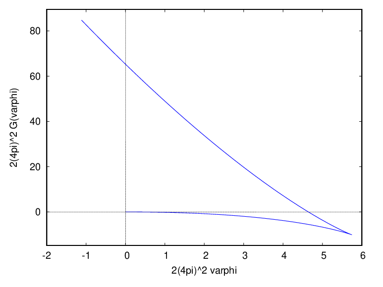
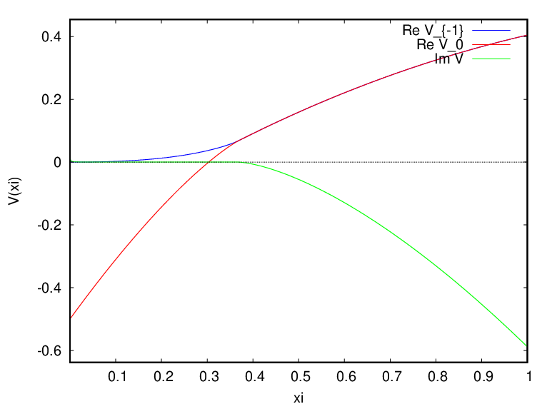
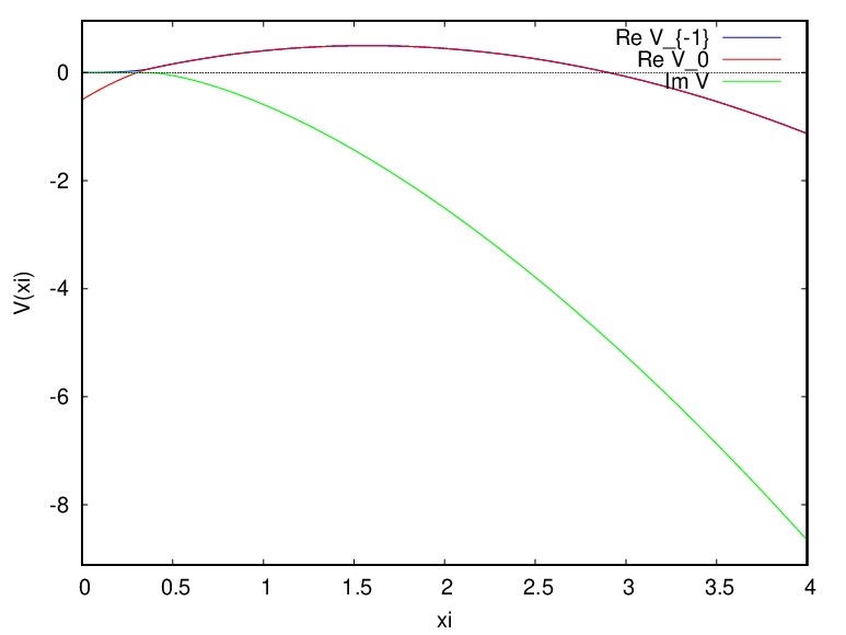
We plot two functions

	$\displaystyle g_{-1}(x)$	$\displaystyle\equiv x^{2}\left(\frac{1}{W_{-1}(-x)}+\frac{1}{2W_{-1}(-x)^{2}}\right)\,,$		(169)
	$\displaystyle g_{0}(x)$	$\displaystyle\equiv x^{2}\left(\frac{1}{W_{0}(-x)}+\frac{1}{2W_{0}(-x)^{2}}\right)\,,$		(170)

for $0<x<1/e$ in Fig. 5. $g_{-1}(x)$ , proportional to our $G_{\mathrm{eff}}(\varphi)$ , is concave, but $g_{0}(x)$ is convex and corresponds to $\sigma<\sigma_{\min}$ , where $F_{\mathrm{eff}}(\sigma)$ is concave, not convex.

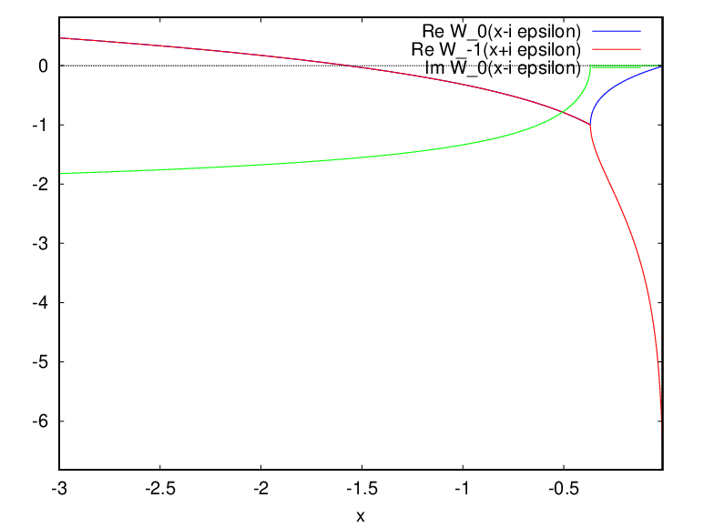
We have found that $\varphi$ has a maximum value $\varphi_{\max}$ beyond which we seem apparently unable to construct $G_{\mathrm{eff}}(\varphi)$ . Let us now speculate that the expression for $G_{\mathrm{eff}}(\varphi)$ may be obtained by analytic continuation for $\xi>\frac{1}{e}$ . $W_{-1}(z)$ has a branch cut along the negative real axis $z<-\frac{1}{e}$ . (See Appendix D for the Riemann sheets of $W$ .) We choose the upper side of the branch cut so that the imaginary part vanishes at $z=-\frac{1}{e}$ .⁶⁶ 6 As is explained in Appendix D, there is another branch cut $-\frac{1}{e}<x<0$ that connects $W_{-1}$ to $W_{1}$ . $W_{-1}$ is real on the upper side of this branch cut. 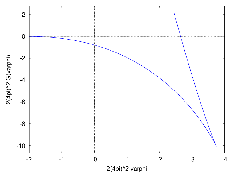Hence, by continuity, it is natural to choose the upper side of the branch cut $x<-\frac{1}{e}$ for the analytic continuation. We plot the real and imaginary parts of

	$\displaystyle V_{-1}(\xi)$	$\displaystyle\equiv-\xi^{2}\left(\frac{1}{W_{-1}(-\xi+i\epsilon)}+\frac{1}{2W_{-1}(-\xi+i\epsilon)^{2}}\right)\,,$		(171)
	$\displaystyle V_{0}(\xi)$	$\displaystyle\equiv-\xi^{2}\left(\frac{1}{W_{0}(-\xi-i\epsilon)}+\frac{1}{2W_{0}(-\xi-i\epsilon)^{2}}\right)\,,$		(172)

in Fig. 6. These two are identical for $\xi>\frac{1}{e}$ .

The effective potential is given by

V_{\mathrm{eff}}(\varphi)=-G_{\mathrm{eff}}(\varphi)=\frac{\Lambda_{L}^{4}}{4(4\pi)^{2}}V_{-1}(\xi)\,.

(173)

$V_{\mathrm{eff}}(\varphi)$ is convex for $\xi<\frac{1}{e}$ , and concave for $\xi>\frac{1}{e}$ . The imaginary part of $V_{\mathrm{eff}}(\varphi)$ implies instability; this must be related to the presence of a tachyon.

In Coleman et al. 1974 it was observed that for $\varphi>\varphi_{\max}$ the effective potential becomes complex, and it acquires a negative imaginary part. They speculate there may be a true minimum of the effective potential at a very large $\varphi$ . Our $V_{\mathrm{eff}}(\varphi)$ obtained by analytic continuation has no such minimum at $\varphi>\varphi_{\max}$ .

Case (b) symmetric phase $f_{1}>0$

We start from

F_{\mathrm{eff}}(f_{1}\mu^{2},f_{2};\sigma)=f_{1}\mu^{2}\sigma+\frac{1}{2}\sigma^{2}\frac{1}{2(4\pi)^{2}}\left(-\ln\frac{-\sigma}{\Lambda_{L}^{2}}+\frac{1}{2}\right)\,,

(155)

and

\varphi=-\frac{d}{d\sigma}F_{\mathrm{eff}}(\sigma)=-f_{1}\mu^{2}+\sigma\frac{1}{2(4\pi)^{2}}\ln\frac{-\sigma}{\Lambda_{L}^{2}}\,,

(174)

which gives

\frac{-\sigma}{\Lambda_{L}^{2}}=\exp\left[W_{-1}\left(-2(4\pi)^{2}\frac{\varphi+f_{1}\mu^{2}}{\Lambda_{L}^{2}}\right)\right]\,.

(175)

$m_{\mathrm{ph}}^{2}$ is defined so that $\varphi=0$ at $\sigma=-m_{\mathrm{ph}}^{2}$ . Hence, we obtain

\frac{m_{\mathrm{ph}}^{2}}{\Lambda_{L}^{2}}=\exp\left[W_{-1}\left(-2(4\pi)^{2}f_{1}\frac{\mu^{2}}{\Lambda_{L}^{2}}\right)\right]=\exp\left[W_{-1}\left(-2(4\pi)^{2}f_{1}e^{-2(4\pi)^{2}f_{2}+A}\right)\right]\,.

(176)

This agrees with (138).

Replacing $-\varphi_{\min}$ by $f_{1}\mu^{2}$ in (167), we obtain

G_{\mathrm{eff}}(\varphi)=\frac{\Lambda_{L}^{4}}{4(4\pi)^{2}}\xi^{2}\left(\frac{1}{W_{-1}(-\xi)}+\frac{1}{2W_{-1}(-\xi)^{2}}\right)\,,

(177)

where

\xi\equiv\frac{2(4\pi)^{2}\left(\varphi+f_{1}\mu^{2}\right)}{\Lambda_{L}^{2}}\,.

(178)

$f_{1}$ simply shifts the plot of $G_{\mathrm{eff}}(\varphi)$ to the left by $f_{1}\mu^{2}$ . At $\varphi=0$ , the slope of the potential is given by

\frac{d}{d\varphi}G_{\mathrm{eff}}(\varphi)\Big|_{\varphi=0}=-m_{\mathrm{ph}}^{2}\,.

(179)

The negative imaginary part of $V_{\mathrm{eff}}=-G_{\mathrm{eff}}$ is developed for $\xi>\frac{1}{e}$ , i.e.,

\varphi>-f_{1}\mu^{2}+\frac{1}{e}\frac{\Lambda_{L}^{2}}{2(4\pi)^{2}}\,.

(180)

VII With a cutoff

To summarize so far, there are problems with the effective action and potential in the naive continuum limit.

1.

The effective action, in particular the two-point vertex of $\varphi$ , suffers from a tachyon pole.
2.

Assuming the analytic continuation for $\varphi>\varphi_{\max}$ is valid, the effective potential $V_{\mathrm{eff}}(\varphi)$ develops a negative imaginary part, and its real part is unbounded from below.

In this section we start from a bare action of the O $(N)$ linear sigma model with a physical cutoff $\Lambda_{0}$ and compute its effective action and potential. We confirm the absence of any of the problems suffered by the naive continuum limit. In the next section we compare the cutoff theory with the naive continuum limit, and show how the problems with the latter arise when the cutoff $\Lambda_{0}$ is raised beyond the Landau pole.

We start from

F_{t=0}[\sigma]=\left(-\frac{1}{4}\int_{p}f(p)+f_{1}\right)\sigma(0)+\frac{f_{2}}{2}\int_{p}\sigma(p)\sigma(-p)\,,

(181)

where

f_{2}>0

(182)

is the inverse of the bare $\phi^{4}$ coupling. Unlike $f_{1},f_{2}$ of the previous sections, $f_{1},f_{2}$ in this section are bare parameters defined at the cutoff scale $\Lambda_{0}$ to be introduced shortly. Let us construct the 1PI action corresponding to (181).

For

-\frac{1}{4}\int_{p}f(p)+f_{1}<0

we define

\varphi_{\min}=\frac{1}{4}\int_{p}f(p)-f_{1}>0\,.

(183)

We obtain

	$\displaystyle\Gamma_{I,t=0}[\varphi]$	$\displaystyle=F_{t=0}[\sigma]+\varphi_{\min}\sigma(0)+\int_{p}\sigma(-p)\left(\varphi(p)-\varphi_{\min}\delta(p)\right)$
		$\displaystyle=-\frac{1}{2f_{2}}\int_{p}\left(\varphi(p)-\varphi_{\min}\delta(p)\right)\left(\varphi(-p)-\varphi_{\min}\delta(-p)\right)\,.$		(184)

This is the action of the O $(N)$ linear sigma model in the broken phase.

For

-\frac{1}{4}\int_{p}f(p)+f_{1}>0

we define $m^{2}$ by

-\frac{1}{4}\int_{p}f(p)+f_{1}-f_{2}m^{2}=0\Longrightarrow m^{2}=\frac{-\frac{1}{4}\int_{p}f(p)+f_{1}}{f_{2}}\,.

(185)

We obtain

	$\displaystyle\Gamma_{I,t=0}[\varphi]$	$\displaystyle=F_{t=0}[\sigma]-m^{2}\varphi(0)+\int_{p}\left(\sigma(-p)+m^{2}\delta(p)\right)\varphi(p)$
		$\displaystyle=-m^{2}\varphi(0)-\frac{1}{2f_{2}}\int_{p}\varphi(p)\varphi(-p)\,.$		(186)

This is the action of the O $(N)$ linear sigma model in the symmetric phase.

Calculating the effective action and potential in the following, we will find that the order parameter is $f_{1}$ , not $f_{1}-\frac{1}{4}\int_{p}f(p)$ . The model is in the broken phase if $f_{1}<0$ , in the symmetric phase if $f_{1}>0$ . We compute the effective action and potential in the two subsections below.

VII.1 Broken phase $f_{1}<0$

Starting from (181), we obtain, for $t>0$ ,

$\displaystyle F_{t}[\sigma]$	$\displaystyle=\left(-\frac{1}{4}\int_{p}f(p)+f_{1}e^{2t}\right)\sigma(0)$
	$\displaystyle\quad+\frac{1}{2}\int_{p}\sigma(p)\sigma(-p)\left(f_{2}+\frac{t}{(4\pi)^{2}}+\mathcal{F}(p)-\mathcal{F}(pe^{-t},-pe^{-t})\right)$
	$\displaystyle\quad+\sum_{n=3}^{\infty}\frac{1}{n!}\int_{p_{1},\cdots,p_{n}}\sigma(p_{1})\cdots\sigma(p_{n})\,\delta\left(\sum_{1}^{n}p_{i}\right)$
	$\displaystyle\qquad\times\left(I_{n}(p_{1},\cdots,p_{n})-e^{-2(n-2)t}I_{n}(p_{1}e^{-t},\cdots,p_{n}e^{-t})\right)\,,$	(187)

where we have used the general formula (47).

The Legendre transform of the effective action is obtained as

F_{\mathrm{eff}}[\sigma]=\lim_{\Lambda\to 0+}F_{t=\ln\frac{\Lambda_{0}}{\Lambda}}[\sigma_{\Lambda}]\,,

(188)

where

\sigma_{\Lambda}(p)=\Lambda^{2}\sigma(p\Lambda)\,.

(189)

We find

$\displaystyle F_{t=\ln\frac{\Lambda_{0}}{\Lambda}}[\sigma_{\Lambda}]$	$\displaystyle=\left(-\frac{1}{4}\int_{p}f(p)+f_{1}\left(\frac{\Lambda_{0}}{\Lambda}\right)^{2}\right)\sigma_{\Lambda}(0)$
	$\displaystyle\quad+\frac{1}{2}\int_{p}\sigma_{\Lambda}(p)\sigma_{\Lambda}(-p)\left(f_{2}+\frac{1}{(4\pi)^{2}}\ln\frac{\Lambda_{0}}{\mu}+\mathcal{F}(p)+\frac{1}{(4\pi)^{2}}\ln\frac{\mu}{\Lambda}\right)+I[\sigma_{\Lambda}]$
	$\displaystyle\quad-\frac{1}{2}\int_{p}\sigma_{\Lambda}(p)\sigma_{\Lambda}(-p)\mathcal{F}\left(p\frac{\Lambda}{\Lambda_{0}}\right)-\sum_{n=3}^{\infty}\frac{1}{2n}\int_{p_{1},\cdots,p_{n}}\sigma_{\Lambda}(p_{1})\cdots\sigma_{\Lambda}(p_{n})\,\delta\left(\sum_{1}^{n}p_{i}\right)$
	$\displaystyle\qquad\times\left(\frac{\Lambda}{\Lambda_{0}}\right)^{2(n-2)}I_{n}\left(p_{1}\frac{\Lambda}{\Lambda_{0}},\cdots,p_{n}\frac{\Lambda}{\Lambda_{0}}\right)\,.$	(190)

Since

\sigma_{\Lambda}(p)=\Lambda^{2}\sigma(p\Lambda)=\frac{\Lambda^{2}}{\Lambda_{0}^{2}}\Lambda_{0}^{2}\sigma\left(p\frac{\Lambda}{\Lambda_{0}}\Lambda_{0}\right)=\frac{\Lambda^{2}}{\Lambda_{0}^{2}}\sigma_{\Lambda_{0}}\left(p\frac{\Lambda}{\Lambda_{0}}\right)\,,

(191)

we obtain

	$\displaystyle\frac{1}{2}\int_{p}\sigma_{\Lambda}(p)\sigma_{\Lambda}(-p)\,\mathcal{F}\left(p\frac{\Lambda}{\Lambda_{0}}\right)$	$\displaystyle=\frac{1}{2}\int_{p}\frac{\Lambda^{4}}{\Lambda_{0}^{4}}\sigma_{\Lambda_{0}}\left(p\frac{\Lambda}{\Lambda_{0}}\right)\sigma_{\Lambda_{0}}\left(-p\frac{\Lambda}{\Lambda_{0}}\right)\,\mathcal{F}\left(p\frac{\Lambda}{\Lambda_{0}}\right)$
		$\displaystyle=\frac{1}{2}\int_{p}\sigma_{\Lambda_{0}}(p)\sigma_{\Lambda_{0}}(-p)\mathcal{F}(p)\,,$		(192)

and

		$\displaystyle\sum_{n=3}^{\infty}\frac{1}{2n}\int_{p_{1},\cdots,p_{n}}\sigma_{\Lambda}(p_{1})\cdots\sigma_{\Lambda}(p_{n})\,\delta\left(\sum_{1}^{n}p_{i}\right)\,\left(\frac{\Lambda}{\Lambda_{0}}\right)^{2(n-2)}I_{n}\left(p_{1}\frac{\Lambda}{\Lambda_{0}},\cdots,p_{n}\frac{\Lambda}{\Lambda_{0}}\right)$
		$\displaystyle=\sum_{n=3}^{\infty}\frac{1}{2n}\int_{p_{1},\cdots,p_{n}}\sigma_{\Lambda_{0}}\left(p_{1}\frac{\Lambda}{\Lambda_{0}}\right)\cdots\sigma_{\Lambda_{0}}\left(p_{n}\frac{\Lambda}{\Lambda_{0}}\right)\,\left(\frac{\Lambda}{\Lambda_{0}}\right)^{4n}\delta\left(\sum_{1}^{n}p_{i}\frac{\Lambda}{\Lambda_{0}}\right)$
		$\displaystyle\qquad\times I_{n}\left(p_{1}\frac{\Lambda}{\Lambda_{0}},\cdots,p_{n}\frac{\Lambda}{\Lambda_{0}}\right)$
		$\displaystyle=\sum_{n=3}^{\infty}\frac{1}{2n}\int_{p_{1},\cdots,p_{n}}\sigma_{\Lambda_{0}}(p_{1})\cdots\sigma_{\Lambda_{0}}(p_{n})\,\delta\left(\sum_{1}^{n}p_{i}\right)\,I_{n}(p_{1},\cdots,p_{n})=I[\sigma_{\Lambda_{0}}]\,.$		(193)

Hence, we can write

$\displaystyle F_{t=\ln\frac{\Lambda_{0}}{\Lambda}}[\sigma_{\Lambda}]$	$\displaystyle=\left(-\frac{1}{4}\int_{p}f(p)+f_{1}\left(\frac{\Lambda_{0}}{\Lambda}\right)^{2}\right)\sigma_{\Lambda}(0)$
	$\displaystyle\quad+\frac{1}{2}\int_{p}\sigma_{\Lambda}(p)\sigma_{\Lambda}(-p)\left(f_{2}+\frac{1}{(4\pi)^{2}}\ln\frac{\Lambda_{0}}{\mu}+\mathcal{F}(p)+\frac{1}{(4\pi)^{2}}\ln\frac{\mu}{\Lambda}\right)+I[\sigma_{\Lambda}]$
	$\displaystyle\quad-\frac{1}{2}\int_{p}\sigma_{\Lambda_{0}}(p)\sigma_{\Lambda_{0}}(-p)\,\mathcal{F}(p)-I[\sigma_{\Lambda_{0}}]\,.$	(194)

Note that the first two lines on the right-hand side is the same as in the naive continuum limit except that $f_{2}$ is replaced by $f_{2}+\frac{1}{(4\pi)^{2}}\ln\frac{\Lambda_{0}}{\mu}$ here. Hence, in the limit $\Lambda\to 0$ , we obtain

$\displaystyle F_{\mathrm{eff}}[\sigma]$	$\displaystyle=-\varphi_{\min}\sigma(0)$
	$\displaystyle\quad+\frac{1}{2}\int_{p}\sigma(p)\sigma(-p)\left(\frac{1}{\lambda}-\frac{1}{(4\pi)^{2}}\ln\frac{p}{\mu}+B-\mathcal{F}\left(\frac{p}{\Lambda_{0}}\right)\right)$
	$\displaystyle\quad+\sum_{n=3}^{\infty}\frac{1}{2n}\int_{p_{1},\cdots,p_{n}}\sigma(p_{1})\cdots\sigma(p_{n})\,\delta\left(\sum_{1}^{n}p_{i}\right)$
	$\displaystyle\qquad\times\left(I_{n,\mathrm{eff}}(p_{1},\cdots,p_{n})-\frac{1}{\Lambda_{0}^{2(n-2)}}I_{n}\left(\frac{p_{1}}{\Lambda_{0}},\cdots,\frac{p_{n}}{\Lambda_{0}}\right)\right)\,,$	(195)

where

	$\displaystyle\varphi_{\min}$	$\displaystyle\equiv-f_{1}\Lambda_{0}^{2}>0\,,$		(196)
	$\displaystyle\lambda$	$\displaystyle\equiv\frac{1}{f_{2}+\frac{1}{(4\pi)^{2}}\ln\frac{\Lambda_{0}}{\mu}}\,,$		(197)

and $I_{n,\mathrm{eff}}$ is given by (118). Fixing $\varphi_{\min}$ and $\lambda$ , we obtain (120) if we take $\Lambda_{0}\to\infty$ naively.

The Legendre transform of (195) gives

$\displaystyle\Gamma_{\mathrm{eff},I}[\varphi]$	$\displaystyle=F_{\mathrm{eff}}[\sigma]+\varphi_{\min}\sigma(0)+\int_{p}\sigma(-p)\left(\varphi(p)-\varphi_{\min}\delta(p)\right)$
	$\displaystyle=\sum_{n=2}^{\infty}\frac{1}{n!}\int_{p_{1},\cdots,p_{n}}\left(\varphi(p_{1})-\varphi_{\min}\delta(p_{1})\right)\cdots\left(\varphi(p_{n})-\varphi_{\min}\delta(p_{n})\right)\,\delta\left(\sum_{1}^{n}p_{i}\right)$
	$\displaystyle\quad\times c_{n,\mathrm{eff}}(p_{1},\cdots,p_{n})\,.$	(198)

where


$\displaystyle c_{2,\mathrm{eff}}(p,-p)$	$\displaystyle=-\frac{1}{\frac{1}{\lambda}-\frac{1}{(4\pi)^{2}}\ln\frac{p}{\mu}+B-\mathcal{F}\left(\frac{p}{\Lambda_{0}}\right)}\,,$	(199a)
$\displaystyle c_{3,\mathrm{eff}}(p_{1},p_{2},p_{3})$	$\displaystyle=\prod_{i=1}^{3}c_{2}(p_{i},-p_{i})\cdot\left[I_{3,\mathrm{eff}}(p_{1},\cdots.p_{n})-\Lambda_{0}^{-2}I_{3}\left(\frac{p_{1}}{\Lambda_{0}},\cdots,\frac{p_{n}}{\Lambda_{0}}\right)\right]\,,$	(199b)

and so on.

We now note that $c_{2,\mathrm{eff}}(p,-p)$ has no tachyon pole since

\frac{1}{\lambda}-\frac{1}{(4\pi)^{2}}\ln\frac{p}{\mu}+B-\mathcal{F}\left(\frac{p}{\Lambda_{0}}\right)>0\,.

(200)

(Proof) In Appendix E we show, for $t>0$ ,

\frac{t}{(4\pi)^{2}}+\mathcal{F}(p)-\mathcal{F}(pe^{-t},-pe^{-t})>0\,.

(201)

This gives, for $\Lambda<\Lambda_{0}$ ,

\frac{1}{(4\pi)^{2}}\ln\frac{\Lambda_{0}}{\Lambda}+\mathcal{F}\left(\frac{p}{\Lambda}\right)-\mathcal{F}\left(\frac{p}{\Lambda_{0}}\right)>0\,.

(202)

We can rewrite this as

\underbrace{\frac{1}{(4\pi)^{2}}\ln\frac{\Lambda_{0}}{\mu}}_{=\frac{1}{\lambda}-f_{2}}\underbrace{-\frac{1}{(4\pi)^{2}}\ln\frac{\Lambda}{\mu}+\mathcal{F}\left(\frac{p}{\Lambda}\right)}_{\overset{\Lambda\to 0}{\longrightarrow}-\frac{1}{(4\pi)^{2}}\ln\frac{p}{\mu}+B}-\mathcal{F}\left(\frac{p}{\Lambda_{0}}\right)>0\,.

(203)

Hence, we obtain

\frac{1}{\lambda}-\frac{1}{(4\pi)^{2}}\ln\frac{p}{\mu}+B-\mathcal{F}\left(\frac{p}{\Lambda_{0}}\right)>f_{2}>0\,.

(204)

(End of Proof)
The asymptotic behavior is given by

c_{2,\mathrm{eff}}(p,-p)\left\{\begin{array}[]{c@{\quad}l}\overset{p\ll\Lambda_{0}}{\longrightarrow}&-\frac{1}{\frac{1}{\lambda}-\frac{1}{(4\pi)^{2}}\ln\frac{p}{\mu}+B}\,,\\ \overset{p\gg\Lambda_{0}}{\longrightarrow}&-\frac{1}{\frac{1}{\lambda}-\frac{1}{(4\pi)^{2}}\ln\frac{\Lambda_{0}}{\mu}}=-\frac{1}{f_{2}}\,.\end{array}\right.

(205)

For $p_{i}\ll\Lambda_{0}$ , the vertex functions $c_{n}(p_{1},\cdots,p_{n})$ of the naive continuum limit are reproduced.

We next consider the effective potential. The Legendre transform of the effective potential is obtained as

F_{\mathrm{eff}}(\sigma)=\lim_{\Lambda\to 0+}\Lambda^{4}F_{t=\ln\frac{\Lambda_{0}}{\Lambda}}\left(\frac{\sigma}{\Lambda^{2}}\right)\,,

(206)

where

$\displaystyle\Lambda^{4}F_{t=\ln\frac{\Lambda_{0}}{\Lambda}}\left(\frac{\sigma}{\Lambda^{2}}\right)$	$\displaystyle=\Lambda^{4}\Bigg[\left(-\frac{1}{4}\int_{p}f(p)+f_{1}\left(\frac{\Lambda_{0}}{\Lambda}\right)^{2}\right)\frac{\sigma}{\Lambda^{2}}+\frac{1}{2}\left(\frac{\sigma}{\Lambda^{2}}\right)^{2}\left(f_{2}+\frac{1}{(4\pi)^{2}}\ln\frac{\Lambda_{0}}{\Lambda}\right)$
	$\displaystyle\qquad\qquad\qquad+I\left(\frac{\sigma}{\Lambda^{2}}\right)-\frac{\Lambda_{0}^{4}}{\Lambda^{4}}I\left(\frac{\sigma}{\Lambda_{0}^{2}}\right)\Bigg]$
	$\displaystyle=\left(-\Lambda^{2}\frac{1}{4}\int_{p}f(p)+f_{1}\Lambda_{0}^{2}\right)\sigma+\frac{1}{2}\sigma^{2}\left(f_{2}+\frac{1}{(4\pi)^{2}}\ln\frac{\Lambda_{0}}{\mu}\right)$
	$\displaystyle\qquad+\Lambda^{4}I\left(\frac{\sigma}{\Lambda^{2}}\right)+\frac{1}{2}\sigma^{2}\frac{1}{(4\pi)^{2}}\ln\frac{\mu}{\Lambda}-\Lambda_{0}^{4}I\left(\frac{\sigma}{\Lambda_{0}^{2}}\right)\,.$	(207)

Taking the limit $\Lambda\to 0+$ , we obtain

F_{\mathrm{eff}}(\sigma)=-\varphi_{\min}\sigma+\frac{1}{\lambda}\frac{1}{2}\sigma^{2}-\frac{1}{2(4\pi)^{2}}\frac{\sigma^{2}}{2}\left(\ln\frac{-\sigma}{\mu^{2}}+A-\frac{1}{2}\right)-\Lambda_{0}^{4}I\left(\frac{\sigma}{\Lambda_{0}^{2}}\right)\,,

(208)

where $\varphi_{\min},\lambda$ are given by (196), (197). This gives

\varphi=\varphi_{\min}-\frac{1}{\lambda}\sigma+\frac{1}{2(4\pi)^{2}}\sigma\left(\ln\frac{-\sigma}{\mu^{2}}+A\right)+\Lambda_{0}^{2}I^{\prime}\left(\frac{\sigma}{\Lambda_{0}^{2}}\right)\,.

(209)

Let us show that $F_{\mathrm{eff}}(\sigma)$ is convex in $\sigma<0$ , i.e., $\varphi$ is a decreasing function of $\sigma<0$ . We wish to show

\frac{d\varphi}{d\sigma}=-f_{2}+\frac{1}{2(4\pi)^{2}}\left(\ln\frac{-\sigma}{\Lambda_{0}^{2}}+A+1\right)+I^{\prime\prime}\left(\frac{\sigma}{\Lambda_{0}^{2}}\right)<0\,.

(210)

(Proof) In Appendix E we show, for $t>0$ ,

-\frac{t}{(4\pi)^{2}}-I^{\prime\prime}(\sigma)+I^{\prime\prime}(\sigma e^{-2t})<0\,.

(211)

Substituting $\frac{\sigma}{\Lambda^{2}}$ for $\sigma$ , and choosing $e^{-t}=\frac{\Lambda}{\Lambda_{0}}$ , we obtain

-\frac{1}{(4\pi)^{2}}\ln\frac{\Lambda_{0}}{\Lambda}-I^{\prime\prime}\left(\frac{\sigma}{\Lambda^{2}}\right)+I^{\prime\prime}\left(\frac{\sigma}{\Lambda_{0}^{2}}\right)<0\,.

(212)

In the limit $\Lambda\to 0+$ , we obtain

\frac{1}{2(4\pi)^{2}}\left(\ln\frac{-\sigma}{\Lambda_{0}^{2}}+A+1\right)+I^{\prime\prime}\left(\frac{\sigma}{\Lambda_{0}^{2}}\right)<0\,.

(213)

Since $f_{2}>0$ , we obtain the desired inequality.
(End of Proof)
Hence, $\varphi$ is well defined in the entire $\sigma<0$ . At $\sigma=0$ , we obtain $\varphi=\varphi_{\min}$ , and $\varphi\to+\infty$ as $\sigma\to-\infty$ . For $-\sigma\gg\Lambda_{0}^{2}$ , we obtain the asymptotic behavior

	$\displaystyle F_{\mathrm{eff}}(\sigma)$	$\displaystyle\overset{-\sigma\gg\Lambda_{0}^{2}}{\longrightarrow}-\varphi_{\min}\sigma+f_{2}\frac{1}{2}\sigma^{2}\,,$		(214)
	$\displaystyle\varphi$	$\displaystyle\overset{-\sigma\gg\Lambda_{0}^{2}}{\longrightarrow}\varphi_{\min}-f_{2}\sigma\,.$		(215)

The 1PI potential is given by

$\displaystyle G_{\mathrm{eff}}(\varphi)$	$\displaystyle=F_{\mathrm{eff}}(\sigma)+\sigma\varphi$
	$\displaystyle=-\frac{1}{2\lambda}\sigma^{2}+\frac{1}{2(4\pi)^{2}}\frac{\sigma^{2}}{2}\left(\ln\frac{-\sigma}{\mu^{2}}+A+\frac{1}{2}\right)-\Lambda_{0}^{4}I\left(\frac{\sigma}{\Lambda_{0}^{2}}\right)+\Lambda_{0}^{2}\sigma I^{\prime}\left(\frac{\sigma}{\Lambda_{0}^{2}}\right)$
	$\displaystyle\overset{-\sigma\gg\Lambda_{0}^{2}}{\longrightarrow}-f_{2}\frac{\sigma^{2}}{2}-\Lambda_{0}^{4}\frac{1}{8}\int_{p}\frac{f(p)}{h(p)}\,.$	(216)

This implies the asymptotic behavior

G_{\mathrm{eff}}(\varphi)\overset{\varphi-\varphi_{\min}\gg f_{2}\Lambda_{0}^{2}}{\longrightarrow}-\frac{1}{2f_{2}}\left(\varphi-\varphi_{\min}\right)^{2}-\Lambda_{0}^{4}\frac{1}{8}\int_{p}\frac{f(p)}{h(p)}\,.

(217)

The additive constant can be ignored. The effective potential reduces to the bare potential for a large field $\varphi$ .

Plot of $V_{\mathrm{eff}}(\varphi)$ for various $\Lambda_{0}$

Let us summarize what is needed to make a plot of the effective potential. For simplicity we take $\varphi_{\min}=0$ . We rewrite (208) and (209) as

	$\displaystyle F_{\mathrm{eff}}(\sigma)$	$\displaystyle=-\frac{1}{2(4\pi)^{2}}\frac{\sigma^{2}}{2}\left(\ln\frac{-\sigma}{\Lambda_{L}^{2}}-\frac{1}{2}\right)-\Lambda_{0}^{4}I\left(\frac{\sigma}{\Lambda_{L}^{2}}\frac{\Lambda_{L}^{2}}{\Lambda_{0}^{2}}\right)\,,$		(218)
	$\displaystyle\varphi$	$\displaystyle=\frac{1}{2(4\pi)^{2}}\sigma\ln\frac{-\sigma}{\Lambda_{L}^{2}}+\Lambda_{0}^{2}I^{\prime}\left(\frac{\sigma}{\Lambda_{L}^{2}}\frac{\Lambda_{L}^{2}}{\Lambda_{0}^{2}}\right)\,,$		(219)

where we have defined

\Lambda_{L}^{2}\equiv\mu^{2}e^{2(4\pi)^{2}\frac{1}{\lambda}-A}\,.

(220)

This $\Lambda_{L}$ is the same as (136) except that $f_{2}$ there is replaced by $\frac{1}{\lambda}$ here.

The definition of $\lambda$ , given by (197), gives

\frac{\Lambda_{0}^{2}}{\Lambda_{L}^{2}}=\exp\left(A-2(4\pi)^{2}f_{2}\right)<e^{A}\,,

(221)

since $f_{2}>0$ . Hence, given $\lambda$ , the largest cutoff we can choose is

\max\Lambda_{0}=\Lambda_{L}\,e^{\frac{A}{2}}=\mu\,e^{(4\pi)^{2}\frac{1}{\lambda}}\,.

(222)

This is the famous Landau pole Landau 1955, corresponding to $f_{2}=0$ . In Fig. 7 we plot the effective potential

V_{\mathrm{eff}}(\varphi)=-G_{\mathrm{eff}}(\varphi)

(223)

for three choices of $\Lambda_{0}$ below the Landau pole:

\Lambda_{0}=(1,0.8,0.6)\Lambda_{L}\,.

(For the cutoff function $R(p)=e^{-p^{2}}$ , we find $A\simeq 0.129$ . Hence, $\Lambda_{L}$ is below the Landau pole.) The $x$ -axis gives

\xi\equiv\frac{2(4\pi)^{2}\varphi}{\Lambda_{L}^{2}}\,.

(224)

(This is the same as (167) except $f_{2}$ there is replaced by $\frac{1}{\lambda}$ here.) We also plot the real part of $V_{\mathrm{eff}}(\varphi)$ in the naive limit that corresponds to $\Lambda_{0}\to+\infty$ :

V^{\mathrm{naive}}_{\mathrm{eff}}(\varphi)=-\frac{1}{2(4\pi)^{2}}\Lambda_{L}^{4}\cdot\frac{\xi^{2}}{2}\left(\frac{1}{W_{-1}(-\xi+i\epsilon)}+\frac{1}{2W_{-1}(-\xi+i\epsilon)^{2}}\right)\,.

(225)

(This is the same as (168)). As $\Lambda_{0}$ decreases, the bare parameter $f_{2}$ gets larger, and $\frac{1}{f_{2}}$ smaller.

VII.2 Symmetric phase $f_{1}>0$

We obtain the physical squared mass $m_{\mathrm{ph}}^{2}$ from

F^{\prime}_{\mathrm{eff}}(\sigma=-m_{\mathrm{ph}}^{2})=0\,,

(226)

where $F_{\mathrm{eff}}$ is given by (208). This gives

f_{1}\Lambda_{0}^{2}-f_{2}m_{\mathrm{ph}}^{2}+\frac{1}{2(4\pi)^{2}}m_{\mathrm{ph}}^{2}\left(\ln\frac{m_{\mathrm{ph}}^{2}}{\Lambda_{0}^{2}}+A\right)-\Lambda_{0}^{2}I^{\prime}\left(-\frac{m_{\mathrm{ph}}^{2}}{\Lambda_{0}^{2}}\right)=0\,.

(227)

For $m_{\mathrm{ph}}^{2}\ll\Lambda_{0}^{2}$ , we obtain approximately

f_{1}\Lambda_{0}^{2}-f_{2}m_{\mathrm{ph}}^{2}+\frac{1}{2(4\pi)^{2}}m_{\mathrm{ph}}^{2}\left(\ln\frac{m_{\mathrm{ph}}^{2}}{\Lambda_{0}^{2}}+A\right)=0\,.

(228)

As long as

2(4\pi)^{2}f_{1}\Lambda_{0}^{2}<\frac{1}{e}\Lambda_{L}^{2}\,,

(229)

where $\Lambda_{L}$ is given by (220), this is solved by

m_{\mathrm{ph}}^{2}=\Lambda_{L}^{2}\exp\left[W_{-1}\left(-\frac{2(4\pi)^{2}f_{1}\Lambda_{0}^{2}}{\Lambda_{L}^{2}}\right)\right]=\frac{2(4\pi)^{2}f_{1}\Lambda_{0}^{2}}{-W_{-1}\left(-\frac{2(4\pi)^{2}f_{1}\Lambda_{0}^{2}}{\Lambda_{L}^{2}}\right)}\,.

(230)

This is the same as (138) except that $f_{1}\mu^{2}$ there is replaced by $f_{1}\Lambda_{0}^{2}$ here.

The calculation of the effective action proceeds the same way as for the broken phase. We merely state the result. We obtain

$\displaystyle F_{\mathrm{eff}}[\sigma]$	$\displaystyle=\frac{1}{2}\int_{p}\left(\sigma(p)+m_{\mathrm{ph}}^{2}\delta(p)\right)\left(\sigma(-p)+m_{\mathrm{ph}}^{2}\delta(p)\right)$
	$\displaystyle\qquad\times\left[\frac{1}{\lambda}+I_{2,\mathrm{eff}}(m_{\mathrm{ph}}^{2};p,-p)-\mathcal{F}\left(\frac{m_{\mathrm{ph}}^{2}}{\Lambda_{0}^{2}};\frac{p}{\Lambda_{0}}\right)\right]$
	$\displaystyle\quad+\sum_{n=3}^{\infty}\frac{1}{2n}\int_{p_{1},\cdots,p_{n}}\left(\sigma(p_{1})+m_{\mathrm{ph}}^{2}\delta(p_{1})\right)\cdots\left(\sigma(p_{n})+m_{\mathrm{ph}}^{2}\delta(p_{n})\right)\,\delta\left(\sum_{1}^{n}p_{i}\right)$
	$\displaystyle\qquad\times\left[I_{n,\mathrm{eff}}(m_{\mathrm{ph}}^{2};p_{1},\cdots,p_{n})-\Lambda_{0}^{-2(n-2)}I_{n}\left(\frac{m_{\mathrm{ph}}^{2}}{\Lambda_{0}^{2}};\frac{p_{1}}{\Lambda_{0}},\cdots,\frac{p_{n}}{\Lambda_{0}}\right)\right]\,,$	(231)

where $I_{2,\mathrm{eff}}$ and $I_{n\geq 3,\mathrm{eff}}$ are defined by (147) and (118), respectively.

The Legendre transformation gives

	$\displaystyle\Gamma_{\mathrm{eff},I}[\varphi]$	$\displaystyle=-m_{\mathrm{ph}}^{2}\varphi(0)+F_{\mathrm{eff}}[\sigma]+\int_{p}\left(\sigma(-p)+m_{\mathrm{ph}}^{2}\delta(p)\right)\varphi(p)$
		$\displaystyle=-m_{\mathrm{ph}}^{2}\varphi(0)+\sum_{n=2}^{\infty}\frac{1}{n!}\int_{p_{1},\cdots,p_{n}}\varphi(p_{1})\cdots\varphi(p_{n})\,\delta\left(\sum_{1}^{n}p_{i}\right)\times c_{n,\mathrm{eff}}\left(m_{\mathrm{ph}}^{2};p_{1},\cdots,p_{n}\right)\,,$		(232)

where


$\displaystyle c_{2,\mathrm{eff}}(m_{\mathrm{ph}}^{2};p,-p)$	$\displaystyle=-\frac{1}{\frac{1}{\lambda}+I_{2,\mathrm{eff}}(m_{\mathrm{ph}}^{2};p,-p)-\mathcal{F}\left(\frac{m_{\mathrm{ph}}^{2}}{\Lambda_{0}^{2}};\frac{p}{\Lambda_{0}}\right)}\,,$	(233a)
$\displaystyle c_{3,\mathrm{eff}}(m_{\mathrm{ph}}^{2};p_{1},p_{2},p_{3})$	$\displaystyle=\prod_{i=1}^{3}c_{2,\mathrm{eff}}(m_{\mathrm{ph}}^{2};p_{i},-p_{i})$
	$\displaystyle\quad\times\left[I_{3,\mathrm{eff}}(m_{\mathrm{ph}}^{2};p_{1},p_{2},p_{3})-\Lambda_{0}^{-2}I_{3}\left(\frac{m_{\mathrm{ph}}^{2}}{\Lambda_{0}^{2}};\frac{p_{1}}{\Lambda_{0}},\frac{p_{2}}{\Lambda_{0}},\frac{p_{3}}{\Lambda_{0}}\right)\right]\,,$	(233b)

and so on.

Let us show $c_{2,\mathrm{eff}}(m_{\mathrm{ph}}^{2};p,-p)$ has no tachyon pole:

\frac{1}{(4\pi)^{2}}\ln\frac{\Lambda_{0}}{\mu}+I_{2}^{\mathrm{cont}}(m_{\mathrm{ph}}^{2};p,-p)-\mathcal{F}\left(\frac{m_{\mathrm{ph}}^{2}}{\Lambda_{0}^{2}};\frac{p}{\Lambda_{0}}\right)>0\,.

(234)

(Proof) In Appendix E we show, for $t>0$ ,

\mathcal{F}(m^{2}e^{2t},pe^{t})+\frac{1}{(4\pi)^{2}}t>\mathcal{F}(m^{2},p)\,.

(235)

Hence, for $\Lambda<\Lambda_{0}$ , we obtain

\mathcal{F}\left(\frac{m^{2}}{\Lambda^{2}},\frac{p}{\Lambda}\right)+\frac{1}{(4\pi)^{2}}\ln\frac{\Lambda_{0}}{\Lambda}-\mathcal{F}\left(\frac{m^{2}}{\Lambda_{0}^{2}},\frac{p}{\Lambda_{0}}\right)>0\,.

(236)

Taking the limit $\Lambda\to 0+$ , and using

I_{2,\mathrm{eff}}(m^{2};p,-p)\equiv\lim_{\Lambda\to 0+}\left(\mathcal{F}\left(\frac{m^{2}}{\Lambda^{2}},\frac{p}{\Lambda}\right)+\frac{1}{(4\pi)^{2}}\ln\frac{\mu}{\Lambda}\right)

we obtain the desired inequality.
(End of Proof)

Thus, we have seen that the effective action is well defined, free from tachyon poles. The 1PI potential $G_{\mathrm{eff}}(\varphi)$ is the same as in the broken phase except for a shift of $\varphi$ by $f_{1}\Lambda_{0}^{2}$ . The slope at $\varphi=0$ gives $-m_{\mathrm{ph}}^{2}$ . All is well.

VIII Comparison with the naive continuum limit

In the previous section we have considered the O $(N)$ linear sigma model with a finite cutoff $\Lambda_{0}$ , and calculated the effective action and effective potential in the large $N$ limit. The model is well defined: the effective action has no tachyon, and the effective potential is real and bounded from below. In this section we would like to see how it goes wrong when we raise the cutoff beyond the Landau pole (222).

We recall how the maximum is derived. The renormalized coupling $\lambda$ is given by

\frac{1}{\lambda}=f_{2}+\frac{1}{(4\pi)^{2}}\ln\frac{\Lambda_{0}}{\mu}

(237)

in the cutoff theory, where $\frac{1}{f_{2}}$ is the bare $\phi^{4}$ coupling at the cutoff scale $\Lambda_{0}$ . Since $f_{2}>0$ , we obtain

\frac{1}{\lambda}>\frac{1}{(4\pi)^{2}}\ln\frac{\Lambda_{0}}{\mu}\Longrightarrow\Lambda_{0}<\mu\,\exp\left(\frac{(4\pi)^{2}}{\lambda}\right)\,.

(238)

In the naive continuum limit, however, we fix $\lambda$ and take $\Lambda_{0}\to+\infty$ , ignoring the above inequality.

Let us take a theory with $\lambda>0$ and a cutoff $\Lambda_{0}$ beyond the Landau pole:

\Lambda_{0}>\mu\exp\left(\frac{(4\pi)^{2}}{\lambda}\right)\,.

(239)

This implies

f_{2}=\frac{1}{\lambda}-\frac{1}{(4\pi)^{2}}\ln\frac{\Lambda_{0}}{\mu}<0\,.

(240)

At the cutoff scale $\Lambda_{0}$ we obtain a bare $\phi^{4}$ potential unbounded from below. This must be the cause of a tachyon pole and the instability of the effective potential. This reasoning is not new; it was first given in Coleman et al. 1974.

VIII.1 Tachyon pole

For simplicity we consider only the critical case $f_{1}=0$ . The effective action is given by

\Gamma_{I,\mathrm{eff}}[\varphi]=\sum_{n=2}^{\infty}\frac{1}{n!}\int_{p_{1},\cdots,p_{n}}\varphi(p_{1})\cdots\varphi(p_{n})\,\delta\left(\sum_{1}^{n}p_{i}\right)\,c_{n,\mathrm{eff}}(p_{1},\cdots,p_{n})\,,

(241)

where


$\displaystyle c_{2,\mathrm{eff}}(p,-p)$	$\displaystyle=-\frac{1}{\frac{1}{\lambda}-\frac{1}{(4\pi)^{2}}\ln\frac{p}{\mu}+B-\mathcal{F}\left(\frac{p}{\Lambda_{0}}\right)}\,,$	(242a)
$\displaystyle c_{3,\mathrm{eff}}(p_{1},p_{2},p_{3})$	$\displaystyle=\prod_{i=1}^{3}c_{2}(p_{i},-p_{i})\cdot\left[I_{3}^{\mathrm{cont}}(p_{1},\cdots.p_{n})-\Lambda_{0}^{-2(n-2)}I_{n}\left(\frac{p_{1}}{\Lambda_{0}},\cdots,\frac{p_{n}}{\Lambda_{0}}\right)\right]\,,$	(242b)

and so on.

We wish to show that $c_{2,\mathrm{eff}}(p,-p)$ has a tachyon pole if $\Lambda_{0}$ satisfies (239). We have

		$\displaystyle\frac{1}{\lambda}-\frac{1}{(4\pi)^{2}}\ln\frac{p}{\mu}+B-\mathcal{F}\left(\frac{p}{\Lambda_{0}}\right)$		(243)
		$\displaystyle=f_{2}-\frac{1}{(4\pi)^{2}}\ln\frac{p}{\Lambda_{0}}+B-\mathcal{F}\left(\frac{p}{\Lambda_{0}}\right)\,,$		(244)

where $f_{2}<0$ . The first inequality in Appendix E gives

0\leq-\frac{1}{(4\pi)^{2}}\ln\frac{p}{\Lambda_{0}}+B-\mathcal{F}\left(\frac{p}{\Lambda_{0}}\right)\longrightarrow\left\{\begin{array}[]{c@{\quad}l}+\infty&(p\to 0)\\ 0&(p\to+\infty)\end{array}\right.\,.

(245)

Hence, $c_{2,\mathrm{eff}}(p,-p)$ must have a tachyon pole.

As $\Lambda_{0}\to+\infty$ , the pole approaches $p=\mu e^{(4\pi)^{2}\left(\frac{1}{\lambda}+B\right)}$ . Let us find the tachyon pole for $\Lambda_{0}$ a little beyond the limit:

f_{2}=\frac{1}{\lambda}-\frac{1}{(4\pi)^{2}}\ln\frac{\Lambda_{0}}{\mu}=-\epsilon\,,

(246)

where $-\epsilon$ is a small negative constant. The pole satisfies

-\frac{1}{(4\pi)^{2}}\ln\frac{p}{\Lambda_{0}}+B-\mathcal{F}\left(\frac{p}{\Lambda_{0}}\right)=\epsilon\ll 1\,.

(247)

For $p\gg\Lambda_{0}$ , we find (Appendix C)

\mathcal{F}\left(\frac{p}{\Lambda_{0}}\right)=-\frac{1}{(4\pi)^{2}}\ln\frac{p}{\Lambda_{0}}+B-\frac{\Lambda_{0}^{2}}{2p^{2}}\int_{q}f(q)\,.

(248)

Hence, we obtain

\frac{\Lambda_{0}^{2}}{2p^{2}}\int_{q}f(q)=\epsilon\Longrightarrow p^{2}=\frac{\Lambda_{0}^{2}}{2\epsilon}\int_{q}f(q)\gg\Lambda_{0}^{2}\,.

(249)

As $\Lambda_{0}$ increases, this should approach the limiting value $p=\mu e^{(4\pi)^{2}\left(\frac{1}{\lambda}+B\right)}$ .

Incidentally, if the cutoff is a little smaller than the Landau pole

f_{2}=\frac{1}{\lambda}-\frac{1}{(4\pi)^{2}}\ln\frac{\Lambda_{0}}{\mu}=\epsilon>0\,,

(250)

there is a bound state pole at

-p^{2}=\frac{\Lambda_{0}^{2}}{2\epsilon}\int_{q}f(q)\gg\Lambda_{0}^{2}\,.

(251)

This turns over to a tachyon as the cutoff crosses the limit. The transition of a bound state to a tachyon has been observed previously in a model of a charged harmonic oscillator in the radiation field Sonoda 2022 and also in a model of harmonic oscillators with a configuration interaction that mimics the Lee model Sonoda 2014.

VIII.2 Instability

The 1PI potential is given by

	$\displaystyle G_{\mathrm{eff}}(\varphi)$	$\displaystyle=F_{\mathrm{eff}}(\sigma)+\sigma\varphi$
		$\displaystyle=-\frac{1}{2}f_{2}\sigma^{2}+\frac{1}{4(4\pi)^{2}}\frac{\sigma^{2}}{2}+\frac{1}{2(4\pi)^{2}}\frac{\sigma^{2}}{2}\left(\ln\frac{-\sigma}{\Lambda_{0}^{2}}+A\right)-\Lambda_{0}^{4}I\left(\frac{\sigma}{\Lambda_{0}^{2}}\right)+\Lambda_{0}^{2}\sigma I^{\prime}\left(\frac{\sigma}{\Lambda_{0}^{2}}\right)\,,$		(252)

where

	$\displaystyle\varphi$	$\displaystyle=-f_{2}\sigma+\frac{1}{2(4\pi)^{2}}\sigma\left(\ln\frac{-\sigma}{\Lambda_{0}^{2}}+A\right)+\Lambda_{0}^{2}I^{\prime}\left(\frac{\sigma}{\Lambda_{0}^{2}}\right)$
		$\displaystyle=-\left(f_{2}+\frac{1}{(4\pi)^{2}}\ln\frac{\Lambda_{0}}{\mu}\right)\sigma+\frac{1}{2(4\pi)^{2}}\sigma\left(\ln\frac{-\sigma}{\mu^{2}}+A\right)+\Lambda_{0}^{2}I^{\prime}\left(\frac{\sigma}{\Lambda_{0}^{2}}\right)\,.$		(253)

We wish to show that there exists $\sigma_{\min}$ where

\frac{d\varphi}{d\sigma}\Big|_{\sigma=\sigma_{\min}}=0\,.

(254)

$\sigma_{\min}$ corresponds to $\varphi_{\max}$ beyond which the effective potential is likely to develop a negative imaginary part. We find

\frac{d\varphi}{d\sigma}=-f_{2}+\frac{1}{2(4\pi)^{2}}\left(\ln\frac{-\sigma}{\Lambda_{0}^{2}}+A+1\right)+I^{\prime\prime}\left(\frac{\sigma}{\Lambda_{0}^{2}}\right)\,,

(255)

where $-f_{2}>0$ . Since

\frac{1}{2(4\pi)^{2}}\left(\ln\frac{-\sigma}{\Lambda_{0}^{2}}+A+1\right)+I^{\prime\prime}\left(\frac{\sigma}{\Lambda_{0}^{2}}\right)\longrightarrow\left\{\begin{array}[]{c@{\quad}l}-\infty&(-\sigma\to 0+)\\ 0&(-\sigma\to+\infty)\end{array}\right.\,,

(256)

there must be such $\sigma_{\min}$ .

Let us find $\sigma_{\min}$ for a very small $-f_{2}=\epsilon>0$ . We expect $-\sigma_{\min}\gg\Lambda_{0}^{2}$ . Using the asymptotic behavior derived in Appendix C

I^{\prime\prime}(\sigma)\overset{-\sigma\gg 1}{\longrightarrow}-\frac{1}{2}\frac{1}{(4\pi)^{2}}\left(\ln(-\sigma)+A+1\right)+\frac{1}{6\sigma^{3}}\int_{q}\frac{f(q)}{h(q)^{2}}\,,

(257)

we obtain

\epsilon+\frac{1}{6}\frac{\Lambda_{0}^{6}}{\sigma_{\min}^{3}}\int_{q}\frac{f(q)}{h(q)^{2}}=0\,.

(258)

Hence,

(-\sigma_{\min})^{3}=\frac{1}{6}\frac{\Lambda_{0}^{6}}{\epsilon}\int_{q}\frac{f(q)}{h(q)^{2}}\Longrightarrow-\sigma_{\min}=\Lambda_{0}^{2}\left(\frac{1}{6\epsilon}\int_{q}\frac{f(q)}{h(q)^{2}}\right)^{\frac{1}{3}}\gg\Lambda_{0}^{2}\,.

(259)

We expect

-\sigma_{\min}\overset{\Lambda_{0}\to+\infty}{\longrightarrow}\frac{1}{e}\Lambda_{L}^{2}=\frac{1}{e}\mu^{2}e^{\frac{2(4\pi)^{2}}{\lambda}-A}\,.

(260)

IX Concluding remarks

We have studied the large $N$ limit of the O $(N)$ linear sigma model in four dimensions, and computed both the effective action and the effective potential by solving the exact renormalization group equations.

For $N=1$ , the absence of a non-trivial continuum limit has recently been given a rigorous mathematical proof Aizenman and Duminil-Copin 2021. The absence is expected of any $N$ , including the large $N$ limit. This implies that, given a finite renormalized coupling $\lambda$ , we cannot raise the cutoff beyond a certain limit. In the large $N$ limit, the maximum cutoff is the Landau pole

\max\left(\Lambda_{0}\right)=\mu e^{\frac{(4\pi)^{2}}{\lambda}}\,,

(222)

where $\mu$ is the renormalization scale $\lambda$ is defined at. In the naive continuum limit, where $\Lambda_{0}$ is taken to infinity while $\lambda$ is kept fixed, we expect problems. The effective potential, continued analytically for a large field, is found unbounded from below with a negative imaginary part. We hope to justify this analytic continuation in a future publication.

Though the introduction of a cutoff $\Lambda_{0}$ helps to set the theory on a firm ground, it has its own problems, such as the existence of a bound state beyond the cutoff scale as shown in Sec. VIII. The nature of the bound state is cutoff dependent.

There is a lesson to learn from our calculations. If the effective potential of a model shows a sign of instability, suspect it is the fault of a naive continuum limit. The model may not be complete; it may be a part of a larger and more complete theory. We think it would be interesting to apply our method to fermionic theories in large $N$ .

Appendix A Transition to the dimensionful convention

We can move back and forth between the dimensionless convention, where the momentum cutoff is $1$ , and the dimensionful convention, where the momentum cutoff is $\Lambda$ , by using a set of very simple rules. We do not specify the space dimension and leave it as $D$ .

Given a solution $\Gamma_{I,t}[\varphi]$ of the ERG equation (20), we define

\Gamma_{I,\Lambda}[\varphi]\equiv\Gamma_{I,t}[\varphi_{\Lambda}]\,,

(261)

where

	$\displaystyle\Lambda$	$\displaystyle=\mu\,e^{-t}\,,$		(262)
	$\displaystyle\varphi_{\Lambda}(p)$	$\displaystyle=\Lambda^{2}\varphi(p\Lambda)\,.$		(263)

Note that

\varphi(p)=\frac{1}{2N}\int_{q}\Phi^{I}(q+p)\Phi^{I}(-q)

(264)

has mass the dimension $-2$ for any $D$ , and $\Phi^{I}(p)$ has the mass dimension $-\frac{D+2}{2}$ .

We have introduced $\mu$ as a physical renormalization scale, corresponding to $t=0$ . $\Gamma_{I,\Lambda}$ satisfies the ERG differential equation

-\Lambda\frac{\partial}{\partial\Lambda}\Gamma_{I,\Lambda}[\varphi]=\frac{1}{2}\int_{p}\Lambda\frac{\partial R_{\Lambda}(p)}{\partial\Lambda}\,\mathcal{G}_{\Lambda;p,-p}[\varphi]\,,

(265)

where

R_{\Lambda}(p)\equiv\Lambda^{2}R(p/\Lambda)\,,

(266)

and

\mathcal{G}_{\Lambda;p,-q}[\varphi]\equiv\Lambda^{-(D+2)}\mathcal{G}_{t;p/\Lambda,-q/\Lambda}[\varphi_{\Lambda}]

(267)

satisfies

\int_{q}\mathcal{G}_{\Lambda;p,-q}[\varphi]\left[\left(q^{2}+R_{\Lambda}(q)\right)\delta(q-r)-\frac{\delta\Gamma_{I,\Lambda}[\varphi]}{\delta\varphi(q-r)}\right]=\delta(p-r)\,.

(268)

In the limit $\Lambda\to 0+$ , we obtain the 1PI generating functional of the correlation functions:

\Gamma_{I,\mathrm{eff}}[\varphi]=\lim_{\Lambda\to 0+}\Gamma_{I,\Lambda}[\varphi]\,.

(269)

Similarly, the Legendre transform of $\Gamma_{I,\Lambda}[\varphi]$ is given by

F_{\Lambda}[\sigma]\equiv F_{t}[\sigma_{\Lambda}]\,,

(270)

where

\sigma_{\Lambda}(p)=\Lambda^{D-2}\sigma(p\Lambda)\,.

(271)

$\Gamma_{I,\Lambda}[\varphi]$ and $F_{\Lambda}[\sigma]$ are related by

\Gamma_{I,\Lambda}[\varphi]=F_{\Lambda}[\sigma]+\int_{p}\sigma(p)\varphi(-p)\,,

(272)

and

\sigma(p)=\frac{\delta\Gamma_{I,\Lambda}[\varphi]}{\delta\varphi(-p)},\quad\varphi(p)=-\frac{\delta F_{\Lambda}[\sigma]}{\delta\sigma(-p)}\,.

(273)

For the 1PI potential, we define

G_{\Lambda}(\varphi)\equiv\Lambda^{D}G_{t}(\varphi_{\Lambda})\,,

(274)

where

\varphi_{\Lambda}\equiv\Lambda^{2-D}\varphi\,.

(275)

The mass dimensions of $\varphi$ and $G_{\Lambda}$ are $D-2$ and $D$ , respectively. The ERG equation

\partial_{t}G_{t}(\varphi)=\left(D-(D-2)\varphi\,\partial_{\varphi}\right)G_{t}(\varphi)+\frac{1}{2}\int_{q}f(q)\frac{\partial_{\varphi}G_{t}(\varphi)}{1-h(q)\partial_{\varphi}G_{t}(\varphi)}

(276)

gives

-\Lambda\partial_{\Lambda}G_{\Lambda}(\varphi)=\frac{1}{2}\int_{q}\frac{\Lambda\partial_{\Lambda}R_{\Lambda}(q)}{q^{2}+R_{\Lambda}(q)}\frac{\partial_{\varphi}G_{\Lambda}(\varphi)}{q^{2}+R_{\Lambda}(q)-\partial_{\varphi}G_{\Lambda}(\varphi)}\,.

(277)

In the limit $\Lambda\to 0+$ , we obtain the effective potential as

V_{\mathrm{eff}}(\varphi)=-G_{\mathrm{eff}}(\varphi)=-\lim_{\Lambda\to 0+}G_{\Lambda}(\varphi)\,.

(278)

Similarly, the Legendre transform of $G_{\Lambda}(\varphi)$ is given by

F_{\Lambda}(\sigma)\equiv\Lambda^{D}F_{t}\left(\sigma_{\Lambda}\right)\,,

(279)

where

\sigma_{\Lambda}\equiv\Lambda^{-2}\sigma\,.

(280)

$\sigma$ has the mass dimension $2$ independent of $D$ . $G_{\Lambda}$ and $F_{\Lambda}$ are related by the Legendre transformation

G_{\Lambda}(\varphi)=F_{\Lambda}(\sigma)+\sigma\varphi\,,

(281)

where

\varphi=-\frac{d}{d\sigma}F_{\Lambda}(\sigma),\quad\sigma=\frac{d}{d\varphi}G_{\Lambda}(\varphi)\,.

(282)

The ERG equation

\partial_{t}F_{t}(\sigma)=\left(D-2\sigma\,\partial_{\sigma}\right)F_{t}(\sigma)+\frac{1}{2}\int_{q}f(q)\frac{\sigma}{1-\sigma h(q)}

(283)

gives

-\Lambda\partial_{\Lambda}F_{\Lambda}(\sigma)=\frac{1}{2}\int_{q}\frac{\Lambda\partial_{\Lambda}R_{\Lambda}(q)}{q^{2}+R_{\Lambda}(q)}\frac{\sigma}{q^{2}+R_{\Lambda}(q)-\sigma}\,.\

(284)

The Legendre transform of $G_{\mathrm{eff}}(\varphi)$ is obtained as

F_{\mathrm{eff}}(\sigma)=\lim_{\Lambda\to 0+}F_{\Lambda}(\sigma)\,.

(285)

Appendix B $I[\sigma]$ and $I(\sigma)$

In this Appendix, the dimensionality of space is fixed as $D=4$ .

B.1 Functional $I[\sigma]$

We define

I[\sigma]\equiv\sum_{n=3}^{\infty}\frac{1}{2n}\int_{p_{1},\cdots,p_{n}}\sigma(p_{1})\cdots\sigma(p_{n})\,\delta\left(\sum_{1}^{n}p_{i}\right)\,I_{n}(p_{1},\cdots,p_{n})\,,

(286)

where

I_{n\geq 3}(p_{1},\cdots,p_{n})\equiv\int_{p}h(p)h(p+p_{1})\cdots h\left(p+\sum_{1}^{n-1}p_{i}\right)\,,

(287)

and the high momentum propagator is defined by

h(p)\equiv\frac{1}{p^{2}+R(p)}\,.

(288)

The cutoff function $R(p)$ is $1$ at $p=0$ and approaches $0$ rapidly at large $p$ . For numerical calculations, we use $R(p)=e^{-p^{2}}$ .

The functional $I[\sigma]$ satisfies

		$\displaystyle\int_{p}(p\cdot\partial_{p}+2)\sigma(p)\cdot\frac{\delta I[\sigma]}{\delta\sigma(p)}$
		$\displaystyle=\frac{1}{2}\int_{p}(p\cdot\partial_{p}-2)R(p)\cdot\left(\mathcal{G}_{p,-p}[\sigma]-h(p)\delta(0)-h(p)^{2}\sigma(0)-h(p)^{2}\int_{q}\sigma(q)h(p+q)\sigma(-q)\right)$
		$\displaystyle=-\frac{1}{2}\int_{p}f(p)\sum_{n=3}^{\infty}\int_{q_{1},\cdots,q_{n}}\,\delta\left(\sum_{1}^{n}q_{i}\right)$
		$\displaystyle\quad\times\sigma(q_{1})h(p+q_{1})\sigma(q_{2})h(p+q_{1}+q_{2})\sigma(q_{3})\cdots\sigma(q_{n-1})h\left(p+\sum_{1}^{n-1}q_{i}\right)\sigma(q_{n})\,,$		(289)

where

f(p)\equiv(2-p\cdot\partial_{p})R(p)\cdot h(p)^{2}>0\,.

(290)

We wish to show

I[\sigma]-I[-m^{2}\delta]-\int_{p}\frac{\delta I[\sigma]}{\delta\sigma(p)}\Big|_{\sigma=-m^{2}\delta}\left(\sigma(p)+m^{2}\delta(p)\right)\\ =I(m^{2})[\sigma+m^{2}\delta]\,,

where the right-hand side is defined by

		$\displaystyle I(m^{2})[\sigma+m^{2}\delta]\equiv\frac{1}{2}\int_{p,q}\left(\mathcal{F}(m^{2};p)-\mathcal{F}(p)\right)\left(\sigma(p)+m^{2}\delta(p)\right)\left(\sigma(-p)+m^{2}\delta(p)\right)$
		$\displaystyle\quad+\sum_{n=3}^{\infty}\frac{1}{2n}\int_{p_{1},\cdots,p_{n}}\delta\left(\sum_{1}^{n}p_{i}\right)\,I_{n}(m^{2};p_{1},\cdots,p_{n})\,\left(\sigma(p_{1})+m^{2}\delta(p_{1})\right)\cdots\left(\sigma(p_{n})+m^{2}\delta(p_{n})\right)\,,$		(291)

and


$\displaystyle h(m^{2},p)$	$\displaystyle\equiv\frac{1}{p^{2}+m^{2}+R(p)}\,,$	(292a)
$\displaystyle\mathcal{F}(p)$	$\displaystyle\equiv\frac{1}{2}\int_{q}h(q)\left(h(q+p)-h(q)\right)\,,$	(292b)
$\displaystyle\mathcal{F}(m^{2};p)$	$\displaystyle\equiv\frac{1}{2}\int_{q}\left(h(m^{2},q)h(m^{2},q+p)-h(q)^{2}\right)\,,$	(292c)
$\displaystyle I_{n\geq 3}(m^{2};p_{1},\cdots,p_{n})$	$\displaystyle\equiv\int_{p}h(m^{2},p)h(m^{2},p+p_{1})\cdots h\left(m^{2},p+\sum_{1}^{n-1}p_{i}\right)\,.$	(292d)

Equivalently, we wish to show

\boxed{I[\sigma-m^{2}\delta]-I[-m^{2}\delta]-\int_{p}\frac{\delta I[\sigma]}{\delta\sigma(p)}\Big|_{\sigma=-m^{2}\delta}\sigma(p)=I(m^{2})[\sigma]\,.}

(293)

Substituting

\sigma(p)\longrightarrow\sigma(p)-m^{2}\delta(p)

(294)

into Eq. (289), we obtain

		$\displaystyle\left(-2m^{2}\partial_{m^{2}}+\int_{p}(p\cdot\partial_{p}+2)\sigma(p)\cdot\frac{\delta}{\delta\sigma(p)}\right)I[\sigma-m^{2}\delta]$
		$\displaystyle=-\frac{1}{2}\int_{p}(2-p\cdot\partial_{p})R(p)\cdot\Big[\mathcal{G}_{p,-p}[\sigma-m^{2}\delta]-h(p)\delta(0)-h(p)^{2}\left(\sigma(0)-m^{2}\delta(0)\right)$
		$\displaystyle\quad-h(p)^{2}\int_{q}\left(\sigma(q)-m^{2}\delta(q)\right)h(p+q)\left(\sigma(-q)-m^{2}\delta(q)\right)\Big]\,,$		(295)

where $\mathcal{G}_{p,-q}[\sigma-m^{2}\delta]$ is determined by

\int_{q}\mathcal{G}_{p,-q}[\sigma-m^{2}\delta]\left[(q^{2}+m^{2}+R(q))\delta(q-r)-\sigma(-q+r)\right]=\delta(p-r)\,.

(296)

(This is obtained from Eq. (27) by the substitution (294).) We can expand

		$\displaystyle\mathcal{G}_{p,-q}[\sigma-m^{2}\delta]=h(m^{2},p)\delta(p-q)+h(m^{2},p)\Big[\sigma(-p+q)$
		$\displaystyle\quad+\int_{p_{1},p_{2}}\sigma(p_{1})h(m^{2},p+p_{1})\sigma(p_{2})\delta(p_{1}+p_{2}+p-q)+\int_{p_{1},p_{2},p_{3}}\sigma(p_{1})h(m^{2},p+p_{1})$
		$\displaystyle\quad\times\sigma(p_{2})h(m^{2},p+p_{1}+p_{2})\sigma(p_{3})\delta(p_{1}+p_{2}+p_{3}+p-q)+\cdots\Big]h(m^{2},q)\,.$		(297)

Expanding (295) up to first order in $\sigma$ , we obtain

		$\displaystyle-2m^{2}\partial_{m^{2}}I[-m^{2}\delta]$
		$\displaystyle=-\frac{1}{2}\int_{p}(2-p\cdot\partial_{p})R(p)\cdot\left[h(m^{2},p)\delta(0)-h(p)\delta(0)+h(p)^{2}m^{2}\delta(0)-h(p)^{3}(m^{2})^{2}\delta(0)\right]\,,$		(298)

and

		$\displaystyle\int_{p}\sigma(p)(-2m^{2}\partial_{m^{2}})\frac{\delta}{\delta\sigma(p)}I[\sigma-m^{2}\delta]\Big\|_{\sigma=0}+\int_{p}(p\cdot\partial_{p}+2)\sigma(p)\cdot\frac{\delta}{\delta\sigma(p)}I[\sigma-m^{2}\delta]\Big\|_{\sigma=0}$
		$\displaystyle=-\frac{1}{2}\int_{p}(2-p\cdot\partial_{p})R(p)\cdot\left[h(m^{2},p)^{2}-h(p)^{2}+2h(p)^{3}m^{2}\right]\sigma(0)\,.$		(299)

Hence, we obtain

		$\displaystyle\left(-2m^{2}\partial_{m^{2}}+\int_{p}(p\cdot\partial_{p}+2)\sigma(p)\cdot\frac{\delta}{\delta\sigma(p)}\right)\left[I[\sigma-m^{2}\delta]-I[-m^{2}\delta]-\int_{q}\sigma(q)\frac{\delta I[\sigma-m^{2}\delta]}{\delta\sigma(q)}\Big\|_{\sigma=0}\right]$
		$\displaystyle=-\frac{1}{2}\int_{p}(2-p\cdot\partial_{p})R(p)\cdot\left(\mathcal{G}_{p,-p}[\sigma-m^{2}\delta]-h(m^{2},p)\delta(0)-h(p)^{2}\int_{q}\sigma(q)h(q+p)\sigma(-q)\right)\,.$		(300)

We now derive the differential equation satisfied by $I(m^{2})[\sigma]$ , and compare the result with (300). Since


		$\displaystyle p\cdot\partial_{p}\mathcal{F}(p)=\frac{1}{2}\int_{q}(p\cdot\partial_{p}+q\cdot\partial_{q}+4)\left[h(q)\left(h(q+p)-h(q)\right)\right]$
		$\displaystyle\quad=\int_{q}f(q)\left(h(q+p)-h(q)\right)=\int_{q}f(q)h(q+p)-\frac{1}{(4\pi)^{2}}\,,$		(301a)
		$\displaystyle\left(p\cdot\partial_{p}+2m^{2}\partial_{m^{2}}\right)\mathcal{F}(m^{2},p)$
		$\displaystyle\quad=\frac{1}{2}\int_{q}\left(p\cdot\partial_{p}+q\cdot\partial_{q}+2m^{2}\partial_{m^{2}}+4\right)\left(h(m^{2},q)h(m^{2},q+p)-h(q)^{2}\right)$
		$\displaystyle\quad=\int_{q}f(m^{2},q)h(m^{2},q+p)-\frac{1}{(4\pi)^{2}}\,,$		(301b)

we obtain

(p\cdot\partial_{p}+2m^{2}\partial_{m^{2}})\left(\mathcal{F}(m^{2},p)-\mathcal{F}(p)\right)=\int_{q}\left(f(m^{2},q)h(m^{2},q+p)-f(q)h(q+p)\right)\,.

(302)

Using

		$\displaystyle\left(\sum_{1}^{n}p_{i}\cdot\partial_{p_{i}}+2m^{2}\partial_{m^{2}}+2(n-2)\right)I_{n}(m^{2};p_{1},\cdots,p_{n})$
		$\displaystyle\quad=\int_{p}\left(p\cdot\partial_{p}+\sum_{1}^{n}p_{i}\cdot\partial_{p_{i}}+2m^{2}\partial_{m^{2}}+2n\right)\left[h(m^{2},p)h(m^{2},p+p_{1})h\left(m^{2},p+\sum_{1}^{n-1}p_{i}\right)\right]$
		$\displaystyle\quad=\int_{p}\Big[f(m^{2},p)h(m^{2},p+p_{1})\cdots h\left(m^{2},p+\sum_{1}^{n-1}p_{i}\right)$
		$\displaystyle\qquad\quad+h(m^{2},p)f(m^{2},p+p_{1})\cdots\ h\left(m^{2},p+\sum_{1}^{n-1}p_{i}\right)+\cdots\Big]\,,$		(303)

we obtain

		$\displaystyle\left(-2m^{2}\partial_{m^{2}}+\int_{p}(p\cdot\partial_{p}+2)\sigma(p)\cdot\frac{\delta}{\delta\sigma(p)}\right)I(m^{2})[\sigma]$
		$\displaystyle=-\frac{1}{2}\int_{p}(2-p\cdot\partial_{p})R(p)\cdot\left(\mathcal{G}_{p,-p}[\sigma-m^{2}\delta]-h(m^{2},p)\delta(0)-h(p)^{2}\int_{q}\sigma(q)h(q+p)\sigma(-q)\right)\,.$		(304)

The right-hand side is the same as that of Eq. (300). The differential equation has a unique analytic solution, and we obtain the desired equality.

B.2 Function $I(\sigma)$

We define

	$\displaystyle I(\sigma)$	$\displaystyle\equiv\frac{1}{2}\int_{p}\left[-\ln\left(1-h(p)\sigma\right)-h(p)\sigma-\frac{1}{2}h(p)^{2}\sigma^{2}\right]$
		$\displaystyle=\sum_{n=3}^{\infty}\frac{1}{2n}I_{n}\cdot\sigma^{n}\,,$		(305)

where

I_{n\geq 3}\equiv\int_{p}h(p)^{n}\,.

(306)

Given an arbitrary $m^{2}>0$ , we would like to show

I(\sigma)-I(-m^{2})-I^{\prime}(-m^{2})(\sigma+m^{2})=I(m^{2};\sigma+m^{2})\,,

(307)

where

$\displaystyle I(m^{2};\sigma+m^{2})$	$\displaystyle\equiv\frac{1}{2}\mathcal{F}_{m^{2}}(\sigma+m^{2})^{2}+\frac{1}{2}\int_{p}\left[-\ln\left(1-h(m^{2},p)(\sigma+m^{2})\right)\right.$
	$\displaystyle\left.\qquad-h(m^{2},p)(\sigma+m^{2})-\frac{1}{2}h(m^{2},p)^{2}(\sigma+m^{2})^{2}\right]$
	$\displaystyle=\frac{1}{2}\mathcal{F}_{m^{2}}(\sigma+m^{2})^{2}+\sum_{n=3}^{\infty}\frac{1}{2n}I_{n}(m^{2})\left(\sigma+m^{2}\right)^{n}\,,$	(308)

and

	$\displaystyle\mathcal{F}_{m^{2}}$	$\displaystyle\equiv\frac{1}{2}\int_{p}\left(h(m^{2},p)^{2}-h(p)^{2}\right)=\mathcal{F}(m^{2};p=0)\,,$		(309)
	$\displaystyle I_{n\geq 3}(m^{2})$	$\displaystyle\equiv\int_{p}h(m^{2},p)^{n}=I_{n}(m^{2};0,\cdots,0)\,.$		(310)

This is a zero momentum version of Eq. (293). Instead of showing that both sides of Eq. (307) satisfy the same differential equation, we prove it directly by computation.

		$\displaystyle I(\sigma)-I(-m^{2})-I^{\prime}(-m^{2})\cdot(\sigma+m^{2})$
		$\displaystyle=\frac{1}{2(4\pi)^{2}}\int_{0}^{\infty}dp^{2}\,p^{2}\left[-\ln\frac{p^{2}-\sigma+R}{p^{2}+R}-\frac{\sigma}{p^{2}+R}-\frac{1}{2}\frac{\sigma^{2}}{(p^{2}+R)^{2}}+\ln\frac{p^{2}+m^{2}+R}{p^{2}+R}\right.$
		$\displaystyle\quad\left.+\frac{-m^{2}}{p^{2}+R}+\frac{1}{2}\frac{(m^{2})^{2}}{(p^{2}+R)^{2}}-(\sigma+m^{2})\left(\frac{1}{p^{2}+m^{2}+R}-\frac{1}{p^{2}+R}+\frac{m^{2}}{(p^{2}+R)^{2}}\right)\right]$
		$\displaystyle=\frac{1}{2(4\pi)^{2}}\int_{0}^{\infty}dp^{2}\,p^{2}\left[-\ln\left(1-\frac{\sigma+m^{2}}{p^{2}+m^{2}+R}\right)-\frac{\sigma+m^{2}}{p^{2}+m^{2}+R}\right.$
		$\displaystyle\quad\left.-\frac{1}{2}(\sigma+m^{2})^{2}\frac{1}{(p^{2}+m^{2}+R)^{2}}+\frac{1}{2}(\sigma+m^{2})^{2}\left(-\frac{1}{(p^{2}+R)^{2}}+\frac{1}{(p^{2}+m^{2}+R)^{2}}\right)\right]$
		$\displaystyle=\frac{1}{2}\int_{p}\left(-\ln\left(1-(\sigma+m^{2})h(m^{2},p)\right)-(\sigma+m^{2})h(m^{2},p)-\frac{1}{2}(\sigma+m^{2})^{2}h(m^{2},p)^{2}\right)$
		$\displaystyle\quad+\frac{1}{2}(\sigma+m^{2})^{2}\cdot\frac{1}{2}\int_{p}\left(h(m^{2},p)^{2}-h(p)^{2}\right)$
		$\displaystyle=I(m^{2};\sigma+m^{2})\,.$		(311)

Appendix C Asymptotic behaviors

C.1 Asymptotic behavior of $I(\sigma)$

To derive the asymptotic behavior of

I(\sigma)\equiv\frac{1}{2}\int_{p}\left(-\ln\left(1-\sigma h(p)\right)-\sigma h(p)-\frac{1}{2}\sigma^{2}h(p)^{2}\right)\,,

(312)

we first derive the differential equation it satisfies. From

\int_{p}\left(p\cdot\partial_{p}+4\right)\left[-\ln\left(1-h(p)\sigma\right)-h(p)\sigma-\frac{1}{2}h(p)^{2}\sigma^{2}\right]=0\,,

(313)

we obtain

	$\displaystyle 2\sigma I^{\prime}(\sigma)-4I(\sigma)$	$\displaystyle=2\sigma^{3}\frac{d}{d\sigma}\left(\frac{1}{\sigma^{2}}I(\sigma)\right)$
		$\displaystyle=\frac{\sigma}{2}\int_{p}f(p)\left(\frac{1}{1-h(p)\sigma}-1-h(p)\sigma\right)\,.$		(314)

For $-\sigma\gg 1$ , we expand the right-hand side to obtain

	$\displaystyle 2\sigma I^{\prime}(\sigma)-4I(\sigma)$	$\displaystyle\overset{-\sigma\gg 1}{\longrightarrow}\frac{\sigma}{2}\int_{p}f(p)\left(-\frac{1}{h(p)\sigma}-\frac{1}{h(p)^{2}\sigma^{2}}-1-h(p)\sigma\right)$
		$\displaystyle=-\frac{1}{2}\int_{p}\frac{f(p)}{h(p)}-\frac{1}{2\sigma}\int_{p}\frac{f(p)}{h(p)^{2}}-\frac{\sigma}{2}\int_{p}f(p)-\frac{\sigma^{2}}{2}\underbrace{\int_{p}f(p)h(p)}_{=\frac{1}{(4\pi)^{2}}}\,.$		(315)

Hence, we obtain

\frac{d}{d\sigma}\left(\frac{1}{\sigma^{2}}I(\sigma)\right)\overset{-\sigma\gg 1}{\longrightarrow}-\frac{1}{4\sigma}\frac{1}{(4\pi)^{2}}-\frac{1}{4\sigma^{2}}\int_{p}f(p)-\frac{1}{4\sigma^{3}}\int_{p}\frac{f(p)}{h(p)}-\frac{1}{4\sigma^{4}}\int_{p}\frac{f(p)}{h(p)^{2}}\,.

(316)

This implies the asymptotic behavior

I(\sigma)\overset{-\sigma\gg 1}{\longrightarrow}-\frac{1}{2(4\pi)^{2}}\frac{\sigma^{2}}{2}\left(\ln(-\sigma)+A-\frac{1}{2}\right)+\frac{1}{4}\sigma\int_{p}f(p)+\frac{1}{8}\int_{p}\frac{f(p)}{h(p)}+\frac{1}{12\sigma}\int_{p}\frac{f(p)}{h(p)^{2}}\,,

(317)

where the constant $A$ depends on the choice of a cutoff function $R$ .

Differentiating the above further, we obtain

$\displaystyle I^{\prime}(\sigma)$	$\displaystyle=\frac{1}{2}\int_{p}\left[\frac{1}{p^{2}+R(p)-\sigma}-h(p)-\sigma h(p)^{2}\right]$
	$\displaystyle\overset{-\sigma\gg 1}{\longrightarrow}-\frac{1}{2(4\pi)^{2}}\sigma\left(\ln(-\sigma)+A\right)+\frac{1}{4}\int_{p}f(p)-\frac{1}{12\sigma^{2}}\int_{p}\frac{f(p)}{h(p)^{2}}\,,$	(318)
$\displaystyle I^{\prime\prime}(\sigma)$	$\displaystyle=\frac{1}{2}\int_{p}\left[\frac{1}{\left(p^{2}+R(p)-\sigma\right)^{2}}-h(p)^{2}\right]$
	$\displaystyle\overset{-\sigma\gg 1}{\longrightarrow}-\frac{1}{2(4\pi)^{2}}\left(\ln(-\sigma)+A+1\right)+\frac{1}{6\sigma^{3}}\int_{p}\frac{f(p)}{h(p)^{2}}\,.$	(319)

We plot $I^{\prime}(\sigma),I^{\prime\prime}(\sigma)$ for the choice $R(p)=e^{-p^{2}}$ in Fig. 8.

C.2 Asymptotic behavior of $\mathcal{F}(p)$

The function

\mathcal{F}(p)\equiv\frac{1}{2}\int_{q}h(q)\left(h(q+p)-h(q)\right)

(320)

satisfies

$\displaystyle p\cdot\partial_{p}\mathcal{F}(p)$	$\displaystyle=\frac{1}{2}\int_{q}(p\cdot\partial_{p}+q\cdot\partial_{q}+4)\left(h(q)h(q+p)-h(q)^{2}\right)$
	$\displaystyle=\int_{q}f(q)\left(h(q+p)-h(q)\right)$
	$\displaystyle\overset{p^{2}\to\infty}{\longrightarrow}\frac{1}{p^{2}}\int_{q}f(q)-\frac{1}{(4\pi)^{2}}\,.$	(321)

This implies

\mathcal{F}(p)\overset{p^{2}\to\infty}{\longrightarrow}-\frac{1}{2(4\pi)^{2}}\ln p^{2}+B-\frac{1}{2p^{2}}\int_{q}f(q)\,,

(322)

where $B$ is a constant dependent on the cutoff function $R$ . Hence, we obtain

\lim_{\Lambda\to 0+}\left(\mathcal{F}\left(\frac{p}{\Lambda}\right)+\frac{1}{(4\pi)^{2}}\ln\frac{\mu}{\Lambda}\right)=-\frac{1}{2(4\pi)^{2}}\ln\frac{p^{2}}{\mu^{2}}+B\,.

(323)

C.3 Asymptotic behavior of $\mathcal{F}_{m^{2}}$

The constant

\mathcal{F}_{m^{2}}\equiv\frac{1}{2}\int_{p}\left(h(m^{2},p)^{2}-h(p)^{2}\right)

(324)

satisfies

$\displaystyle 2m^{2}\partial_{m^{2}}\mathcal{F}_{m^{2}}$	$\displaystyle=\frac{1}{2}\int_{p}\left(p\cdot\partial_{p}+2m^{2}\partial_{m^{2}}+4\right)\left(h(m^{2},p)^{2}-h(p)^{2}\right)$
	$\displaystyle=\int_{p}\left(f(m^{2},p)h(m^{2},p)-f(p)h(p)\right)$
	$\displaystyle\overset{m^{2}\gg 1}{\longrightarrow}-\frac{1}{(4\pi)^{2}}\,.$	(325)

Hence,

\mathcal{F}_{m^{2}}\overset{m^{2}\to+\infty}{\longrightarrow}-\frac{1}{2(4\pi)^{2}}\ln m^{2}+C\,,

(326)

where $C$ is a constant dependent on the cutoff function $R$ .

Appendix D Riemann sheets of the Lambert $W$ function

The main branch $W(z)=W_{0}(z)$ is real on the real axis $-\frac{1}{e}<z=x<+\infty$ . The lower branch $W_{-1}(z)$ is also real for $W_{-1}(x+i\epsilon)$ where $-\frac{1}{e}<x<0$ . The $W_{0}$ branch is connected to the $W_{\pm 1}$ branches so that for $x<-\frac{1}{e}$


$\displaystyle W_{0}(x-i\epsilon)$	$\displaystyle=W_{-1}(x+i\epsilon)\,,$	(327a)
$\displaystyle W_{0}(x+i\epsilon)$	$\displaystyle=W_{1}(x-i\epsilon)\,.$	(327b)

We also find

W_{0}(x+i\epsilon)=W_{0}(x-i\epsilon)^{*}\quad\left(x<-\frac{1}{\epsilon}\right)\,.

(328)

The $W_{-1}$ branch has more complicated branch cuts.


$\displaystyle W_{-1}(x+i\epsilon)$	$\displaystyle=W_{0}(x-i\epsilon)\quad\left(x<-\frac{1}{e}\right)\,,$	(329a)
$\displaystyle W_{-1}(x+i\epsilon)$	$\displaystyle=W_{1}(x-i\epsilon)\quad\left(-\frac{1}{e}<x<0\right)\,,$	(329b)
$\displaystyle W_{-1}(x-i\epsilon)$	$\displaystyle=W_{-2}(x+i\epsilon)\quad\left(x<0\right)\,.$	(329c)

The cut between the $W_{-1}$ and $W_{-2}$ branches lies along the entire negative real axis $x<0$ .

We plot $W_{0}(x-i\epsilon),W_{-1}(x+i\epsilon)$ for $-3<x<0$ in Fig. 10.

More details can be found in Corless et al. 1996 and Wikipedia 2023.

Appendix E Inequalities

E.1 First inequality

We wish to show, for $t>0$ ,

S(t,p)\equiv\frac{t}{(4\pi)^{2}}+\mathcal{F}(p)-\mathcal{F}(pe^{-t},-pe^{-t})>0\,.

(330)

Note

S(0,p)=0\,.

(331)

Since

p\cdot\partial_{p}\mathcal{F}(p)=\int_{q}f(q)h(q+p)-\frac{1}{(4\pi)^{2}}\,,

(332)

we obtain

\partial_{t}S(t,p)=\frac{1}{(4\pi)^{2}}+p\cdot\partial_{p}\mathcal{F}(pe^{-t},-pe^{-t})=\int_{q}f(q)h(q+pe^{-t})>0\,.

(333)

Hence, $S(t,p)$ is an increasing positive function of $t$ .

S(t,p)>0\quad(t>0)\,.

(334)

For large $t\gg 1$ , we find

S(t,p)\simeq\frac{t}{(4\pi)^{2}}+\mathcal{F}(p)\,.

(335)

For $p\gg e^{t}$ , we find

S(t,p)\simeq\frac{t}{(4\pi)^{2}}-\frac{1}{(4\pi)^{2}}\ln p+\frac{1}{(4\pi)^{2}}\ln(pe^{-t})=0\,.

(336)

E.2 Second inequality

We wish to show, for $\sigma<0$ ,

\frac{1}{(4\pi)^{2}}+2\sigma\frac{d}{d\sigma}I^{\prime\prime}(\sigma)>0\,.

(337)

The asymptotic behavior (319) implies that the left-hand side vanishes as $\sigma\to-\infty$ . Now, differentiating

2\sigma I^{\prime}(\sigma)-4I(\sigma)=\frac{\sigma}{2}\int_{p}f(p)\left(\frac{1}{1-h(p)\sigma}-1-h(p)\sigma\right)\,,

(338)

which is (314), twice with respect to $\sigma$ , we obtain

2\sigma I^{\prime\prime\prime}(\sigma)+\frac{1}{(4\pi)^{2}}=\int_{p}f(p)\frac{h(p)}{(1-h(p)\sigma)^{3}}>0\,.

(339)

Hence, the left-hand side of (337) is increasing, and the inequality holds.

E.3 Third inequality

For $t>0$ , we wish to show

\mathcal{F}(m^{2}e^{2t},pe^{t})+\frac{1}{(4\pi)^{2}}t-\mathcal{F}(m^{2},p)>0\,.

(340)

To prove this we first note the lhs vanishes at $t=0$ . We then note

	$\displaystyle\partial_{t}\left(\mathcal{F}(m^{2}e^{2t},pe^{t})+\frac{1}{(4\pi)^{2}}t\right)$	$\displaystyle=\int_{q}f(m^{2}e^{2t},q)h(m^{2}e^{2t},q+pe^{t})$
		$\displaystyle=\int_{q}(2-q\cdot\partial_{q})R(q)\cdot h(m^{2},q)^{2}h(m^{2}e^{2t},q+pe^{t})>0\,.$		(341)

This proves the inequality.

Acknowledgements.

I would like to thank Prof. Bala Sathiapalan of the Institute for Mathematical Sciences in Chennai for his help in the early stage of the work and his continued support and encouragement.

References

Berlin and Kac (1952) T. H. Berlin and M. Kac, “The spherical model of a ferromagnet,” Phys. Rev. 86, 821–835 (1952).
Stanley (1968) H. E. Stanley, “Spherical model as the limit of infinite spin dimensionality,” Phys. Rev. 176, 718–722 (1968).
Ma (1973) Shang-keng Ma, “Introduction to the renormalization group,” Rev. Mod. Phys. 45, 589–614 (1973).
Wilson (1973) Kenneth G. Wilson, “Quantum field theory models in less than four-dimensions,” Phys. Rev. D 7, 2911–2926 (1973).
Moshe and Zinn-Justin (2003) Moshe Moshe and Jean Zinn-Justin, “Quantum field theory in the large N limit: A Review,” Phys.Rept. 385, 69–228 (2003), arXiv:hep-th/0306133 [hep-th] .
Dolan and Jackiw (1974) L. Dolan and R. Jackiw, “Symmetry Behavior at Finite Temperature,” Phys. Rev. D 9, 3320–3341 (1974).
Schnitzer (1974a) Howard J. Schnitzer, “Nonperturbative Effective Potential for Lambda phi**4 Theory in the Many Field Limit,” Phys. Rev. D 10, 1800 (1974a).
Schnitzer (1974b) Howard J. Schnitzer, “The Hartree Approximation in Relativistic Field Theory,” Phys. Rev. D 10, 2042 (1974b).
Coleman et al. (1974) S. R. Coleman, R. Jackiw, and H. D. Politzer, “Spontaneous Symmetry Breaking in the O(N) Model for Large N,” Phys. Rev. D 10, 2491 (1974) (1974).
Corless et al. (1996) R. M. Corless, G. H. Gonnet, D. E. G. Hare, D. J. Jeffrey, and D. E. Knuth, “On the Lambert $W$ function,” Adv. Comput. Math. 5, 329–359 (1996).
Wikipedia (2023) Wikipedia, “Lambert $W$ function — Wikipedia, the free encyclopedia,” http://en.wikipedia.org/w/index.php?title=Lambert%20W%20function&oldid=1139586360 (2023).
Sonoda (2013) Hidenori Sonoda, “Analytic form of the effective potential in the large $N$ limit of a real scalar theory in four dimensions,” (2013), arXiv:1302.6059 [hep-th] .
Wilson and Kogut (1974) K.G. Wilson and John B. Kogut, “The Renormalization group and the epsilon expansion,” Phys. Rept. 12, 75–199 (1974).
Morris (1994) Tim R. Morris, “The Exact renormalization group and approximate solutions,” Int. J. Mod. Phys. A 9, 2411–2450 (1994), arXiv:hep-ph/9308265 .
Becchi (1996) C. Becchi, “On the construction of renormalized gauge theories using renormalization group techniques,” (1996), arXiv:hep-th/9607188 .
Berges et al. (2002) Juergen Berges, Nikolaos Tetradis, and Christof Wetterich, “Nonperturbative renormalization flow in quantum field theory and statistical physics,” Phys. Rept. 363, 223–386 (2002), arXiv:hep-ph/0005122 .
Pawlowski (2007) Jan M. Pawlowski, “Aspects of the functional renormalisation group,” Annals Phys. 322, 2831–2915 (2007), arXiv:hep-th/0512261 .
Gies (2012) Holger Gies, “Introduction to the functional RG and applications to gauge theories,” Lect. Notes Phys. 852, 287–348 (2012), arXiv:hep-ph/0611146 .
Igarashi et al. (2010) Yuji Igarashi, Katsumi Itoh, and Hidenori Sonoda, “Realization of Symmetry in the ERG Approach to Quantum Field Theory,” Prog. Theor. Phys. Suppl. 181, 1–166 (2010), arXiv:0909.0327 [hep-th] .
Rosten (2012) Oliver J. Rosten, “Fundamentals of the Exact Renormalization Group,” Phys. Rept. 511, 177–272 (2012), arXiv:1003.1366 [hep-th] .
Dupuis et al. (2021) N. Dupuis, L. Canet, A. Eichhorn, W. Metzner, J. M. Pawlowski, M. Tissier, and N. Wschebor, “The nonperturbative functional renormalization group and its applications,” Phys. Rept. 910, 1–114 (2021), arXiv:2006.04853 [cond-mat.stat-mech] .
Sonoda (2015) H. Sonoda, “Equivalence of Wilson Actions,” PTEP 2015, 103B01 (2015), arXiv:1503.08578 [hep-th] .
Wetterich (1993) Christof Wetterich, “Exact evolution equation for the effective potential,” Phys. Lett. B 301, 90–94 (1993), arXiv:1710.05815 [hep-th] .
D’Attanasio and Morris (1997) Marco D’Attanasio and Tim R. Morris, “Large N and the renormalization group,” Phys. Lett. B 409, 363–370 (1997), arXiv:hep-th/9704094 .
Sonoda (2017) H. Sonoda, “The generating functional of correlation functions as a high momentum limit of a Wilson action,” PTEP 2017, 123B01 (2017), arXiv:1706.00198 [hep-th] .
Morris and Turner (1998) Tim R. Morris and Michael D. Turner, “Derivative expansion of the renormalization group in O(N) scalar field theory,” Nucl. Phys. B 509, 637–661 (1998), arXiv:hep-th/9704202 .
Litim and Trott (2018) Daniel F. Litim and Matthew J. Trott, “Asymptotic safety of scalar field theories,” Phys. Rev. D 98, 125006 (2018), arXiv:1810.01678 [hep-th] .
Blaizot et al. (2006) J. P. Blaizot, Ramon Mendez Galain, and Nicolas Wschebor, “A New method to solve the non perturbative renormalization group equations,” Phys. Lett. B 632, 571–578 (2006), arXiv:hep-th/0503103 .
Landau (1955) L. D. Landau, in Niels Bohr and the Development of Physics, edited by W. Pauli (McGraw-Hill, New York, 1955) pp. 52–69.
Sonoda (2022) Hidenori Sonoda, “Renormalization for a model of photon scattering off a charged harmonic oscillator,” (2022), arXiv:2212.13475 [quant-ph] .
Sonoda (2014) H. Sonoda, “Renormalization for free harmonic oscillators,” Phys. Rev. D 89, 047702 (2014), arXiv:1311.6936 [hep-th] .
Aizenman and Duminil-Copin (2021) Michael Aizenman and Hugo Duminil-Copin, “Marginal triviality of the scaling limits of critical 4D Ising and $\lambda\phi_{4}^{4}$ models,” Annals of Mathematics 194, 163 – 235 (2021).

Exact Renormalization Group in Large NNPreprint: KOBE-TH-23-02

Abstract

Keywords:

I Introduction

II Short overview of the ERG formalism

III Solving the ERG equation in D=4D=4

III.1 General solution for D=4D=4

III.2 1PI potential

III.3 Convexity of FtF_{t}

IV Absence of a continuum limit

General properties of Gt=TT​(φ)G_{t=T}^{T}(\varphi)

Case (a) f1<14​∫pf⁡(p)f_{1}<\frac{1}{4}\int_{p}f(p)

Tachyon pole

Case (b) f1>14​∫pf⁡(p)f_{1}>\frac{1}{4}\int_{p}f(p)

V Effective action of the naive continuum limit

Case (a) broken phase f1<0f_{1}<0

Case (b) symmetric phase f1>0f_{1}>0

VI Effective potential of the naive continuum limit

Case (a) broken phase f1<0f_{1}<0

Case (b) symmetric phase f1>0f_{1}>0

VII With a cutoff

VII.1 Broken phase f1<0f_{1}<0

Plot of Veff​(φ)V_{\mathrm{eff}}(\varphi) for various Λ0\Lambda_{0}

VII.2 Symmetric phase f1>0f_{1}>0

VIII Comparison with the naive continuum limit

VIII.1 Tachyon pole

VIII.2 Instability

IX Concluding remarks

Appendix A Transition to the dimensionful convention

Appendix B I⁡[σ]I[\sigma] and I⁡(σ)I(\sigma)

B.1 Functional I⁡[σ]I[\sigma]

B.2 Function I⁡(σ)I(\sigma)

Appendix C Asymptotic behaviors

C.1 Asymptotic behavior of I⁡(σ)I(\sigma)

C.2 Asymptotic behavior of ℱ⁡(p)\mathcal{F}(p)

C.3 Asymptotic behavior of ℱm2\mathcal{F}_{m^{2}}

Appendix D Riemann sheets of the Lambert WW function

Appendix E Inequalities

E.1 First inequality

E.2 Second inequality

E.3 Third inequality

Acknowledgements.

References

Exact Renormalization Group in Large $N$ Preprint: KOBE-TH-23-02

III Solving the ERG equation in $D=4$

III.1 General solution for $D=4$

III.3 Convexity of $F_{t}$

General properties of $G_{t=T}^{T}(\varphi)$

Case (a) $f_{1}<\frac{1}{4}\int_{p}f(p)$

Case (b) $f_{1}>\frac{1}{4}\int_{p}f(p)$

Case (a) broken phase $f_{1}<0$

Case (b) symmetric phase $f_{1}>0$

Case (a) broken phase $f_{1}<0$

Case (b) symmetric phase $f_{1}>0$

VII.1 Broken phase $f_{1}<0$

Plot of $V_{\mathrm{eff}}(\varphi)$ for various $\Lambda_{0}$

VII.2 Symmetric phase $f_{1}>0$

Appendix B $I[\sigma]$ and $I(\sigma)$

B.1 Functional $I[\sigma]$

B.2 Function $I(\sigma)$

C.1 Asymptotic behavior of $I(\sigma)$

C.2 Asymptotic behavior of $\mathcal{F}(p)$

C.3 Asymptotic behavior of $\mathcal{F}_{m^{2}}$

Appendix D Riemann sheets of the Lambert $W$ function